J. Fluid Mech. (2005), vol. 545, pp. 213–243. c 2005 Cambridge University Press doi:10.1017/S0022112005006439 Printed in the United Kingdom 213 Linear and nonlinear convection in solidifying ternary alloys By D. M. ANDERSON 1 AND T. P. SCHULZE 2 1 Department of Mathematical Sciences, George Mason University, Fairfax, VA 22030, USA 2 Department of Mathematics, University of Tennessee, Knoxville, TN 37996-1300, USA (Received 3 June 2004 and in revised form 9 May 2005) In this paper we consider buoyancy-driven flow and directional solidification of a ternary alloy in two dimensions. A steady flow can be established by forcing liquid downward at an average rate V through a temperature gradient that is fixed in the laboratory frame of reference and spans both the eutectic and liquidus temperature of the material being solidified. Our results include both a linear stability analysis and numerical solution of the governing equations for finite-amplitude steady states. The ternary system is characterized by two distinct mushy zones – a primary layer with dendrites composed of a single species and, beneath the primary layer, a secondary layer with a dendritic region composed of two species. The two layers have independent effective Rayleigh numbers, which allows for a variety of convection scenarios. 1. Introduction While convection during the solidification of binary alloys has been the focus of attention for a number of years (for reviews see Worster 1997, 2000; Davis 2001), investigation of multi-component materials is a more recent development. The interest in multi-component alloys stems from both the relevance to metallurgy and geophysics and from the emergence of new phenomena in these more complicated systems. In this paper, we aim to explore convection in mushy layers with substructure due to the presence of three species. Invariably, this structure emerges as the result of one material solidifying or precipitating at higher temperatures than the other two. Under typical growth conditions, the resulting interface is highly unstable and leads rapidly to the formation of a layer of dendrites. Upon further cooling, a second dendritic layer composed of two solid species begins to form. Finally, upon being cooled below the ternary eutectic temperature, all three species completely solidify. This double mushy layer geometry was identified experimentally by Aitta, Huppert & Worster (2001a,b) in the aqueous ternary system water–potassium nitrate–sodium nitrate (H 2 O–KNO 3 – NaNO 3 ). Aitta et al. and Anderson (2003) speculated on the possible convective behaviour in this system. In particular, the following four configurations were anti- cipated: both mushy layers are convectively unstable, only the primary mushy layer is unstable, only the secondary mushy layer is unstable, and both mushy layers are stable. Experimental work by Thompson et al. (2003b) on the aqueous ternary system H 2 O–KNO 3 –NaNO 3 described a convection scenario in which the primary mushy layer was unstable and the secondary mushy layer was stable and non-convective. In these experiments, convection in the primary and liquid layers reduced the unstable concentration gradient and, after a transient period of convection, the growth of the
doi:10.1017/S0022112005006439 Printed in the United Kingdom
213
Linear and nonlinear convection in solidifyingternary alloys
By D. M. ANDERSON1 AND T. P. SCHULZE2
1Department of Mathematical Sciences, George Mason University, Fairfax, VA 22030, USA2Department of Mathematics, University of Tennessee, Knoxville, TN 37996-1300, USA
(Received 3 June 2004 and in revised form 9 May 2005)
In this paper we consider buoyancy-driven flow and directional solidification of aternary alloy in two dimensions. A steady flow can be established by forcing liquiddownward at an average rate V through a temperature gradient that is fixed in thelaboratory frame of reference and spans both the eutectic and liquidus temperatureof the material being solidified. Our results include both a linear stability analysisand numerical solution of the governing equations for finite-amplitude steady states.The ternary system is characterized by two distinct mushy zones – a primary layerwith dendrites composed of a single species and, beneath the primary layer, asecondary layer with a dendritic region composed of two species. The two layers haveindependent effective Rayleigh numbers, which allows for a variety of convectionscenarios.
1. IntroductionWhile convection during the solidification of binary alloys has been the focus of
attention for a number of years (for reviews see Worster 1997, 2000; Davis 2001),investigation of multi-component materials is a more recent development. The interestin multi-component alloys stems from both the relevance to metallurgy and geophysicsand from the emergence of new phenomena in these more complicated systems.
In this paper, we aim to explore convection in mushy layers with substructure dueto the presence of three species. Invariably, this structure emerges as the result of onematerial solidifying or precipitating at higher temperatures than the other two. Undertypical growth conditions, the resulting interface is highly unstable and leads rapidlyto the formation of a layer of dendrites. Upon further cooling, a second dendritic layercomposed of two solid species begins to form. Finally, upon being cooled below theternary eutectic temperature, all three species completely solidify. This double mushylayer geometry was identified experimentally by Aitta, Huppert & Worster (2001a, b)in the aqueous ternary system water–potassium nitrate–sodium nitrate (H2O–KNO3–NaNO3). Aitta et al. and Anderson (2003) speculated on the possible convectivebehaviour in this system. In particular, the following four configurations were anti-cipated: both mushy layers are convectively unstable, only the primary mushy layer isunstable, only the secondary mushy layer is unstable, and both mushy layers are stable.
Experimental work by Thompson et al. (2003b) on the aqueous ternary systemH2O–KNO3–NaNO3 described a convection scenario in which the primary mushylayer was unstable and the secondary mushy layer was stable and non-convective. Inthese experiments, convection in the primary and liquid layers reduced the unstableconcentration gradient and, after a transient period of convection, the growth of the
214 D. M. Anderson and T. P. Schulze
secondary mushy layer overtook the primary layer and the system underwent a transi-tion to a non-convecting state. These authors also developed a global conservationmodel to describe the system in this regime and were able to obtain good agreementwith the experimentally observed growth characteristics by incorporating into themodel the measured heat and solute fluxes. Another related experimental system,examined by Bloomfield & Huppert (2003), is the aqueous system H2O–CuSO4–Na2SO4. These authors assessed regimes of thermal and compositional buoyancy fora configuration in which the system was cooled on the side.
A number of diverse models have been used to study ternary alloys, with differencesthat are dictated in large part by the complexity of the equilibrium phase diagramunder consideration. Krane, Incropera & Gaskell (1997) have developed a ternaryalloy model and have performed two- and three-dimensional simulations of convectivepatterns and macrosegregation for the ternary alloy lead–antimony–tin (Pb–Sb–Sn)(Krane & Incropera 1997; Krane, Incropera & Gaskell 1998). Felicelli, Poirier &Heinrich (1997, 1998) have performed simulations for selected ternary and quaternaryalloys in two and three dimensions. Computations of micro- and macrosegregation innickel-based superalloys and the associated mushy-layer evolution that incorporate aphase equilibrium subroutine for nickel-based superalloys (Boettinger et al. 1995) havebeen performed by Schneider et al. (1997). Beckermann, Gu & Boettinger et al. (2000)described experiments and computations in which a single Rayleigh number wasused to characterize and predict chimney convection in nickel-based superalloys. Theaqueous ternary system considered by Aitta et al. (2001a,b) is notable in the companyof its metallurgical counterparts in that the underlying ternary phase diagram is readilydefined by only a small number of simple expressions (for details see next section).The simplicity of the phase diagram for this system, as well as the potential for furtherlaboratory experiments, has encouraged a number of recent investigations. Anderson(2003) developed a model for diffusion-controlled (non-convecting) solidification ofa ternary alloy and identified similarity solutions for solidification from a cooledboundary. Thompson, Huppert & Worster (2003a) developed a related model basedon global conservation arguments. In both of these papers, a detailed characterizationof the non-convecting states was given. We shall make use of this relatively simplephase diagram in the present paper so that our focus can be directed toward theconvective phenomena occurring in the system.
Following a well-established tradition of binary solidification work, we shall con-sider a ‘crystal pulling’ configuration, also known as ‘directional’ solidification. Theidea is to force material at a uniform mass flux through a temperature gradient thatis fixed in a laboratory frame of reference. Linear stability analyses (Worster 1992;Chen, Lu & Yang 1994; Emms & Fowler 1994; Anderson & Worster 1996), weaklynonlinear analyses (Amberg & Homsy 1993; Anderson & Worster 1995; Chung &Chen 2000; Riahi 2002) and nonlinear studies (Schulze & Worster 1998, 1999, 2001;Chung & Worster 2002) of directional solidification of convecting binary alloys havebeen carefully investigated. Among these, the linear stability analysis of Worster(1992) and the nonlinear study of Schulze & Worster (1999) are closely related to thepresent study.
For the case of ternary alloys, the most closely related study is that of Anderson(2003), who examined the similarity solution for non-convecting solidification from afixed cold boundary. Much of the intuition gained from the previous work on ternaryalloys can be applied here, but the present configuration differs from that examinedby Anderson in that here, non-convecting solutions can be expressed independentlyof time (in a moving frame), and hence are well-suited for stability analyses. We shall
Convection in ternary alloys 215
explore both the linear stability of this system with respect to solutal convection andthe nonlinear behaviour of the system by computational means.
Some of the results we describe here can be compared with previous work byMcKibbin & O’Sullivan (1980, 1981), who considered the onset and nonlinear develop-ment of convection in a layered porous medium heated from below in a box of finitewidth. They described two- and three-layer systems in which individual layer thick-nesses and permeabilities were prescribed independently. A temperature gradient wasimposed across the entire system and either a constant pressure or zero mass fluxcondition was imposed at the upper boundary. Their results included the followingobservations: (i) onset of convection tends to be similar to that of a homogeneoussystem if the permeability contrast between layers is not large, (ii) permeabilitycontrast between layers can lead to localization of convection in a higher permeabilitylayer, (iii) localization of the flow in a relatively thin layer tends to increase the criticalRayleigh number and increase the wavenumber of the flow pattern, and (iv) criticalRayleigh numbers for an impermeable top boundary are larger than those for theconstant-pressure top boundary. Nield & Bejan (1999) summarize a number of otherrelated calculations on convection in layered porous media.
There are several important differences between the layered systems with constantpermeabilities, just described, and the present work. (i) The concentration, ratherthan thermal, gradients control the onset and nature of convection and there are twoindependent Rayleigh numbers that characterize the system. (ii) Base state propertiessuch as the mushy-layer thicknesses and non-uniform permeability profiles, which mayvary broadly from one base state to the next, also play a major role. (iii) The interfacesare free boundaries in our analysis and may evolve to highly nonlinear states. (iv) Thepresent porous layers are reactive: the solid fraction, and hence permeability, variesin space and time and the convection under consideration leads generally to localdissolution or additional growth of solid. Some of the consequences of this evolvingstructure, which we address further below, are the formations of inclusions in theprimary and secondary mushy layers in the ternary alloy system.
Our paper is organized as follows. In § 2, we briefly review the ternary phasediagram and describe the governing equations. In § 3, we identify the basic statesolution and investigate its stability. In § 4, we describe the numerical techniques usedto find nonlinear steady states. In § 5, we describe the results, both linear and nonlinear,arrived at by these methods. In § 6, we present our conclusions.
2. Formulation2.1. Ternary phase diagram
The ternary phase diagram identifies the equilibrium phase of a material at a giventemperature and composition. The simplified ternary phase diagram we consider hereis the same as that used by Anderson (2003) and is loosely based on the experimentalsystem H2O–KNO3–NaNO3 considered by Aitta et al. (2001a); this follows the moregeneral description of Smallman (1985). The phase diagram we consider makes use oftwo simplifying assumptions: there are no solid solutions – that is, complete immisci-bility in the solid phases, and there exist linear relations between temperature andcompositions along the liquidus surface and cotectic lines. Both of these assumptionsare more representative of aqueous solutions than of metallic systems, which tendto have extremely complicated phase diagrams. The first assumption provides animportant simplification in that the amount of material released upon re-dissolutioncan be ascertained from the local solid fraction(s) without knowledge of the
216 D. M. Anderson and T. P. Schulze
EBC
EAC
EAB
P
S
E
B
CA
Figure 1. A projection of a ternary phase diagram onto the base-plane, where speciescompositions are indicated by the convention described in the text. The labelled points P,S and E correspond to the state of the system at the primary, secondary and eutectic fronts.
thermodynamic conditions under which the material was solidified, i.e. the systemdoes not exhibit a history-dependence. The second assumption will provide a simplerelationship between liquid compositions and the temperature when an additionalassumption of local equilibrium is invoked below.
In a full ternary phase diagram, the coordinates in a triangular base indicatethe composition while an axis orthogonal to this base represents the temperature.Figure 1 shows the compositional axes in the phase diagram under consideration.We denote the liquid compositions of components A, B and C by A, B and C,which are typically measured in wt % and are normalized here so that A+ B + C =1,and the temperature by T . The three corners correspond to the pure materials A, Band C. Each side represents the composition associated with a binary eutectic phasediagram. For example, the A–B side has C = 0 and the point marked EAB correspondsto the binary eutectic point of the A–B system. Along each side of the ternary phasediagram, cotectic curves extend from the binary eutectic points into the interior of thephase diagram and demark boundaries of three liquidus surfaces. The three cotecticcurves join together at the ternary eutectic point where the temperature is TE and thecompositions are AE , BE and CE . The temperatures along the liquidus surface andcotectic boundary are specified below in terms of the composition.
A material element moving with the liquid through the primary and secondarymushy layers can be identified with a solidification path in the ternary phase diagram.Consider a liquid phase ternary alloy that upon cooling reaches the point P (seefigure 1) on a liquidus surface. Upon further cooling, solid A, composed of pure A,solidifies to form the dendritic solid in the primary mushy layer while the componentsB and C are rejected into the residual liquid. The result of this is an increase of
Convection in ternary alloys 217
component B and C in the liquid and corresponds to a path which descends alongthe liquidus surface toward point S on the cotectic curve. In the absence of flowand solute diffusion, this path corresponds to a ‘tie-line’, along which the ratio ofB and C remains fixed. In the present study, although flow is considered, we findthat the tie-line constraint can still be applied (see § 2.2) (Further evidence supportingthe tie-line condition follows from the experimental measurements reported by Aittaet al. (2001a, b) for diffusion limited regimes and by Thompson et al. (2003b) forconvective regimes; both references show clearly that the liquid compositions in theprimary mushy layer follow a tie-line to a very good approximation.) Once the cotecticboundary is reached at point S, solidification continues with solid A (pure A) and solidB (pure B) forming the dendritic solid of the secondary mushy layer. In the secondarymushy layer the liquid compositions follow the cotectic curve toward the ternaryeutectic point (point E). At the eutectic point, the remaining liquid solidifies to forma eutectic solid composed of solids A, B and C. We denote the local volume fractionof solids A, B and C by φA, φB and φC , the total solid fraction by φ = φA + φB +φC
and the liquid fraction by χ = 1 −φ.The calculations described in the present paper require the definition of only one
liquidus surface and cotectic boundary and so, without loss of generality, we focuson the liquidus surface associated with corner A and the cotectic line associatedwith the A–B side of the phase diagram. We express these conditions in terms of adimensionless temperature T = (T − T P )/�T , where �T = T P − T E is the temperaturedifference across both mushy layers defined in terms of the temperature at the primarymushy layer front T P and the temperature at the eutectic front T E . This implies thatthe dimensionless temperature at the primary mushy layer front is zero and thedimensionless eutectic temperature is − 1. We define the liquidus surface by theequation
T L(A, B) = −1 + MA(A − AE) + MB(B − BE), (2.1)
and the cotectic line by the two equations
A = AC(T ) = AE +1
MCA
(T + 1) , B = BC(T ) = BE +1
MCB
(T + 1). (2.2)
The quantities MA, MB , MCA and MC
B represent the various liquidus and cotectic slopes,made dimensionless with respect to the temperature difference �T , whose values canbe given in terms of three points on the liquidus surface and cotectic line; we usepoint P (where T = 0), point EAB (where T = T AB) and point E (where T = − 1).Requiring that point P lies on the liquidus surface leads to
1 = MA(AP − AE) + MB(BP − BE). (2.3)
Requiring that the cotectic line pass through the binary eutectic point EAB leads to
MCA =
T AB + 1
AAB − AE, MC
B =T AB + 1
BAB − BE, (2.4)
where T AB , AAB and BAB are the values of dimensionless temperature T andcompositions A and B at the binary eutectic point EAB . A fourth relation followsfrom substituting (2.2) into (2.1); this recognizes that the cotectic line is part of theliquidus surface:
1 =MA
MCA
+MB
MCB
. (2.5)
218 D. M. Anderson and T. P. Schulze
We shall consider a compositionally-symmetric ternary phase diagram where AE =BE = 1/3, AAB = BAB = 1/2, AAC = 1/2 and BAC = 0. If we consider symmetry withrespect to temperature, the binary eutectic temperatures on the A–B and A–C sidesof the phase diagram are equal, T AB = T AC , and the equations above can be simplifiedfurther, provided a special choice for T AB is made. In the fully symmetric case, then,we find that MB = 0, MA = MC
A = MCB = 1/(AP − 1/3) and that T AB = − 1 +MA/6. That
a specific value of T AB is required for symmetry reflects the fact that while we usethree points to specify the liquidus plane, an additional constraint at a fourth pointon the plane (the temperature at the A–C binary eutectic) is applied to maintainsymmetry.
2.2. Governing equations
In this paper, we consider the two-dimensional flow and directional solidification of aternary alloy in the region 0 <z <H . This region contains three layers: a liquid layerin hP < z <H , a primary mushy layer in hS < z < hP and a secondary mushy layerin 0 <z <hS . A steady flow can be established within this domain by forcing liquiddownward at an average rate V through a temperature gradient that is fixed in thelaboratory frame of reference and spans both the eutectic and liquidus temperatureof the material being solidified. We shall assume there is no latent heat releasedupon solidification, there is no solute diffusion, there is no density change uponsolidification, the system is in local equilibrium so that the temperature and speciesconcentrations are coupled through the liquidus surface and cotectic line in theequilibrium phase diagram, and that the thermal properties are constant and equalfor all species and phases. Further, we assume the liquid density depends linearly ontemperature and composition
ρ = ρ0(1 + α(T − T P ) + βAA + βBB),
where ρ0 is a reference density, α is a thermal expansion coefficient, and βA andβB model the change in density with species composition. Finally, we employ theBoussinesq approximation.
In addition to the thermodynamic variables defined above, we decompose the fluid
motion into a portion due to the uniform translation of the system, −V k, and a fluxdriven by buoyancy u. Since we have subtracted the uniform motion of the solidphase, this buoyancy-driven flux is also the Darcy flux – the flux of fluid with respectto a stationary solid phase. In the liquid, u reduces to the portion of the fluid velocitydriven by buoyancy. We shall represent this quantity using a streamfunction so thatu = {−ψz, ψx} = ∇ × (ψj ). Thus, in the absence of convection, we will have u =0,which corresponds to a uniform downward volume flux of material at rate V .
The variables are made dimensionless using the scalings
u =uV
, x =x
κ/V, T =
T − T P
�T, p =
p
µκ/Π0
, t =t
V 2/κ,
where κ is the thermal diffusivity, µ is the dynamic viscosity and Π0 is a referencepermeability. These scaling closely follow those used by Schulze & Worster (1999),with the exception of the compositions, which we do not rescale. The non-dimensionalgroups that are formed as a result of these scalings are three Rayleigh numbers anda Darcy number:
Ra =αgΠ0�T
νV, RaA =
βAgΠ0
νV, RaB =
βBgΠ0
νV, Da =
Π0V2
κ2,
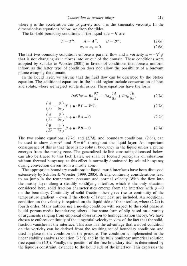
Convection in ternary alloys 219
where g is the acceleration due to gravity and ν is the kinematic viscosity. In thedimensionless equations below, we drop the tildes.
The far-field boundary conditions in the liquid at z = H are
T = T H , A = AH, B = BH, (2.6a)
ψz = ωz = 0. (2.6b)
The last two boundary conditions enforce a parallel flow and a vorticity ω = − ∇2ψ
that is not changing as it moves into or out of the domain. These conditions wereadopted by Schulze & Worster (2001) in favour of conditions that force a uniforminflow, as the latter type of condition does not allow the possibility of a buoyantplume escaping the domain.
In the liquid layer, we assume that the fluid flow can be described by the Stokesequation. The additional equations in the liquid region include conservation of heatand solute, where we neglect solute diffusion. These equations have the form
Da∇4ψ = Ra∂T
∂x+ RaA
∂A
∂x+ RaB
∂B
∂x, (2.7a)(
∂
∂t− ∂
∂z
)T + u · ∇T = ∇2T , (2.7b)(
∂
∂t− ∂
∂z
)A + u · ∇A = 0, (2.7c)(
∂
∂t− ∂
∂z
)B + u · ∇B = 0. (2.7d)
The two solute equations, (2.7c) and (2.7d), and boundary conditions, (2.6a), canbe used to show A= AH and B =BH throughout the liquid layer. An importantconsequence of this is that there is no solutal buoyancy in the liquid unless a plumeemerges from the mushy zone. The generalized tie-line constraint, discussed below,can also be traced to this fact. Later, we shall be focused principally on situationswithout thermal buoyancy, as this effect is normally dominated by solutal buoyancyduring convection driven from a mushy zone.
The appropriate boundary conditions at liquid–mush interfaces have been discussedextensively by Schulze & Worster (1999, 2005). Briefly, continuity considerations leadto no jump in the temperature, pressure and normal velocity. With the flow intothe mushy layer along a steadily solidifying interface, which is the only situationconsidered here, solid fraction characteristics emerge from the interface with φ =0on the boundary. Continuity of solid fraction then gives rise to continuity of thetemperature gradient – even if the effects of latent heat are included. An additionalcondition on the velocity is required on the liquid side of the interface, where (2.7a) isfourth order. Many authors use a no-slip condition with respect to the solid phase atliquid–porous media boundaries; others allow some form of slip based on a varietyof arguments ranging from empirical observation to homogenization theory. We havechosen to enforce continuity of the tangential velocity in view of the fact that the solid-fraction vanishes at the interface. This also has the advantage that a novel conditionon the vorticity can be derived from the resulting set of boundary conditions andused in place of the condition on the pressure. This condition is implemented in thelinear stability analysis (equation (3.8d)) and in the fully nonlinear numerical solution(see equation (4.3)). Finally, the position of the free-boundary itself is determined bythe liquidus constraint, extended to the liquid side of the interface. This expresses the
220 D. M. Anderson and T. P. Schulze
notion that the dendrites expand as far as possible in order to eliminate constitutionalundercooling in the liquid (Worster 1986). Thus, owing to a combination of scalingand the uniform inlet concentration mentioned above, the interface is pinned to theT = 0 isotherm. Taken together, these considerations lead to the following conditionsapplied at z = hP :
Turning to the primary mushy zone, we discuss some general consequences of theassumption of local equilibrium throughout the primary mushy layer before givingthe full set of governing equations. In particular, we show that a tie-line constraint canbe applied in this case. We follow the example of models used for binary alloys andassume that the compositions and temperature are constrained to the liquidus surface,T = T L(A, B). Thus the temperature and composition do not evolve independentlyand the solid fraction must adjust to maintain conservation of species according to(
∂
∂t− ∂
∂z
)A + u · ∇A = 0, (2.9a)(
∂
∂t− ∂
∂z
)B + u · ∇B = 0, (2.9b)
where associated bulk compositions are defined as
A = χA + φA, B = χB + φB. (2.10)
Together, equations (2.9a) and (2.9b) imply a generalized tie-line constraint where theratio of the compositions of passive species – B and C under our present conventions–remains fixed within the primary mushy layer along paths that move with the liquidvelocity. To see why this must hold, it is easier to work with the compositions of thepassive species. We may replace B with χB , and similarly for species C, but not forspecies A, as φA is non-zero in the primary mushy layer. These replacements yield anequation of the form
χ
(∂
∂t− ∂
∂z
)B + B
(∂
∂t− ∂
∂z
)χ + u · ∇B = 0,
and similarly for C. Eliminating (∂/∂t − ∂/∂z) χ from these two equations leads to,after some manipulation, a single equation of the form(
∂
∂t− ∂
∂z+
uχ
· ∇)
B
C= 0. (2.11)
The operator in this equation can be interpreted as a total derivative moving with
an average liquid velocity u/χ − k in the laboratory frame of reference, implyingthat the ratio of B and C is invariant moving with the liquid phase. Since theirinlet compositions are in a fixed ratio across the top of the primary mushy layer,they remain that way within this layer. With both the liquidus constraint and tie-line constraint (2.11) enforced within the primary layer, all of the compositions aredetermined from the temperature field and solute conservation can be used as anevolution equation for the solid fraction. This is why there are no boundary conditionslisted in (2.8) for the concentration fields. It is important to note that the tie-lineconstraint does not apply in cases where solute diffusion is present (Anderson 2003)and must be modified in situations where fluid enters a mushy zone along a boundarywith varying concentration ratios. This type of situation would be encountered, for
Convection in ternary alloys 221
example, after a primary mush inclusion has formed within the secondary mush owingto re-dissolution of the secondary species.
The governing equations in the primary mushy layer are then Darcy’s equation,which we recast in terms of the streamfunction after taking its curl, conservation ofheat and solute species A, the tie-line and liquidus constraints:
∇2ψ = −RaP Π∂T
∂x+
∇Π · ∇ψ
Π, (2.12a)(
∂
∂t− ∂
∂z
)T + u · ∇T = ∇2T , (2.12b)(
∂
∂t− ∂
∂z
)A + u · ∇A = 0, (2.12c)
B =BP
1 − AP(1 − A), (2.12d)
T = T L(A, B), (2.12e)
where Π is the dimensionless permeability function whose form is specified in (2.18).Accompanying these equations is φB = 0 so that φA + χ =1 throughout the primarymushy layer. We emphasis that the relations (2.10) between bulk composition andsolid fraction allow us to interpret (2.12c) as an equation for φA (or equivalentlyχ) and the tie-line and liquidus constraints (2.12d) and (2.12e) as equations for thecompositions A and B . Another important consequence of the tie-line and liquidusconstraints is that a single effective Rayleigh number appears in the momentumequation (2.12a) for the primary mushy layer:
RaP = Ra +RaA(1 − AP ) − RaBBP
MA(1 − AP ) − MBBP. (2.13)
Following arguments similar to those presented above, the boundary conditions atthe mush–mush interface z =hS are
Note that the temperature T S can be deduced by identifying the intersection of thetie-line and the cotectic constraints on the phase diagram and extending the latterconstraint to apply on the primary mushy-layer side of the interface. This generalizesthe notion of marginal equilibrium by assuming that the secondary mushy-layerexpands just enough to relieve any supercooling. Also, for the mush–mush interface inthe present case, the condition of continuous pressure across the interface is equivalentto continuity of tangential velocity when the solid fraction (and hence permeabilities)and species concentrations are also continuous. This is seen by using Darcy’s equationto transfer the continuity of the pressure (and hence pressure gradient) along theinterface to the velocity field. In the work of McKibbin & O’Sullivan (1980), whoaddressed convection in layered porous media of different permeability values, thecondition of pressure continuity does not reduce to continuity of tangential velocity.
The governing equations in the secondary mushy layer are the same as in theprimary mushy layer with the exception that two cotectic constraints replace theliquidus and tie-line constraints and both solute balance equations are required to
222 D. M. Anderson and T. P. Schulze
evolve the two solid fractions φA and φB:
∇2ψ = −RaSΠ∂T
∂x+
∇Π · ∇ψ
Π, (2.15a)(
∂
∂t− ∂
∂z
)T + u · ∇T = ∇2T , (2.15b)(
∂
∂t− ∂
∂z
)A + u · ∇A = 0, (2.15c)(
∂
∂t− ∂
∂z
)B + u · ∇B = 0, (2.15d)
A = AC(T ), (2.15e)
B = BC(T ), (2.15f)
where a second effective Rayleigh number can be identified
RaS = Ra +RaA
MCA
+RaB
MCB
. (2.16)
The boundary conditions at the eutectic interface z = 0 are simply
T = −1, u · n = 0. (2.17)
Note that by definition of the cotectic lines, A= AE and B = BE automatically whenT = − 1. If the z =0 boundary were held at a temperature below the eutectic, thesolid–mush interface would become an additional free- boundary requiring a full setof matching conditions.
Finally, in the work that follows we take the dimensionless permeability to be
Π(χ) = χ3. (2.18)
3. Linear stability analysisWe begin to examine the convective properties of the system in § 2 by way of a
linear stability analysis. In § 3.1 we describe the base state solution, in § 3.2 we outlinethe linearized equations and in § 3.3 we describe the numerical method used to solvethem.
3.1. Base state
The base state is a solution of the governing equations that is one dimensional, steadyin the moving frame and has no buoyancy-driven flow (u = 0). We denote the basestate with overbars. In the liquid layer hP � z � H ,
T = T H − T H
(e−z − e−H
e−hP − e−H
), (3.1a)
A = AH, B = BH . (3.1b)
In the primary mushy layer hS � z � hP ,
T = T S
(e−z − e−hP
e−hS − e−hP
), (3.2a)
χ =MA(AH − 1) + MBBH
MA(AE − 1) + MBBE + 1 + T, (3.2b)
Convection in ternary alloys 223
A =AH − 1
χ+ 1, (3.2c)
B =BH
χ, (3.2d)
and φA =1 − χ , φB = φC = 0, where the cotectic constraints can be used to show that
T S = −1 + MCB
(BH
χS− BE
), (3.3a)
χS =MC
A (AH − 1) − MCB BH
MCA (AE − 1) − MC
B BE. (3.3b)
In the secondary mushy layer 0 � z � hS ,
T = T S − (T S + 1)
(e−z − e−hS
1 − e−hS
), (3.4a)
A = AC(T ), (3.4b)
B = BC(T ), (3.4c)
χ =1 − AH − BH
1 − A − B, (3.4d)
φA = AH − Aχ , (3.4e)
φB = 1 − χ − φA. (3.4f)
Finally, upon applying the thermal gradient jump conditions at z = hP and z = hS wefind that these interface positions are given by
hP = ln
(T H + 1
T H + e−H
), (3.5a)
hS = ln
(T H + 1
T H − T S + e−H (T S + 1)
). (3.5b)
3.2. Linearized equations
We examine the linear stability of this base-state solution by introducing infinitesimalperturbations and linearizing the system of governing equations with respect to theseperturbations. Together, the base states and the perturbations in terms of normalmodes take the form T (x, z, t) = T (z) + T (z)eσ teiαx , ψ(x, z, t) = 0 + iψ(z)eσ teiαx andhP (x, t) = hP + hP eσ teiαx .
The linearized system of equations is given below. In this case the compositionperturbations can be decoupled from the remaining variables. In fact, in the liquidlayer, A= B = 0. The far-field boundary conditions in the liquid at z = H are
T =dψ
dz=
d3ψ
dz3= 0. (3.6)
The linearized equations in the liquid are
d4ψ
dz4− 2α2 dψ
dz2+ α4ψ − αRa
DaT = 0, (3.7a)
d2T
dz2+
dT
dz− α2T + α
dT
dzψ = σ T . (3.7b)
224 D. M. Anderson and T. P. Schulze
The linearized boundary conditions for the perturbed quantities at z = hP are
[T ]+− =
[dT
dz
]+
−= [ψ]+− =
[dψ
dz
]+
−= 0, (3.8a)
T + hP dT
dz= 0, (3.8b)(
χ + hP dχ
dz
)∣∣∣∣−
= 0, (3.8c)
dψ
dz
∣∣∣∣∣−
− Da
(α2 dψ
dz− d3ψ
dz3
)∣∣∣∣∣+
= 0. (3.8d)
The linearized equations in the primary mushy layer are
d2ψ
dz2− 1
Π(χ )
dΠ(χ )
dχ
dχ
dz
dψ
dz− α2ψ + αRaP Π(χ )T = 0, (3.9a)
d2T
dz2+
dT
dz− α2T + α
dT
dzψ = σ T , (3.9b)
d
dz[χ T + (T − T A)χ ] + α
dT
dzψ = σ [χ T + (T − T A)χ ], (3.9c)
where T A = − 1 +MA(1 − AE) − MBBE .The linearized boundary conditions for the perturbed quantities at z = hS are
[T ]+− =
[dT
dz
]+
−
= [ψ]+− =
[dψ
dz
]+
−
= 0, (3.10a)
T + hS dT
dz= 0, (3.10b)[
χ + hS dχ
dz
]+
−= 0, (3.10c)(
φA + hS dφA
dz
)∣∣∣∣−
= 0. (3.10d)
The linearized equations in the secondary mushy layer are
d2ψ
dz2− 1
Π(χ )
dΠ(χ )
dχ
dχ
dz
dψ
dz− α2ψ + αRaSΠ(χ )T = 0, (3.11a)
d2T
dz2+
dT
dz− α2T + α
dT
dzψ = σ T , (3.11b)
d
dz
[χ T + (T − T �
A)χ + MCA φA
]+ α
dT
dzψ = σ
[χ T + (T − T �
A)χ + MCA φA
],
(3.11c)
d
dz
[χ T + (T − T �
B)χ − MCB φA
]+ α
dT
dzψ = σ
[χ T + (T − T �
B)χ − MCB φA
],
(3.11d)
where T �A = − 1 − MC
AAE and T �B = − 1 − MC
B (1 − BE).
Convection in ternary alloys 225
The linearized boundary conditions for the perturbed quantities at z =0 are
T = ψ = 0. (3.12)
3.3. Linearized equations: solution method
We solve this linear system by implementing a pseudo-spectral Chebyshev method(Trefethen 2000). We outline some of the key steps below. First, we rescale each layeronto the interval − 1 � z′ � 1, where
z′ =2(z − h+)
h+ − h− + 1. (3.13)
In the liquid layer h+ =H and h− = hP , in the primary mushy layer h+ = hP andh− = hS and in the secondary mushy layer h+ = hS and h− =0. We discretize thevertical coordinate in each of the three layers (liquid, primary mush and secondarymush) using Chebyshev points
z′j = cos
(jπ
N
), j = 0, 1, 2, . . . , N, (3.14)
where N =NL in the liquid layer, N =NP in the primary layer and N = NS in thesecondary layer. The dependent variables are also discretized. Derivatives are com-puted using Chebyshev differentiation matrices as described by the Matlab imple-mentation cheb.m in Trefethen. This discretization leads to a generalized eigenvalueproblem of the form Ay = σBy where A and B are (2NL +3NP + 4NS + 11) × (2NL +3NP +4NS + 11) matrices representing the system of linearized equations and boun-dary conditions, σ is the eigenvalue and y is a vector whose components are thediscretized values of the dependent variables through the liquid layer, primary mushylayer and secondary mushy layer, including the unknowns hP and hS . The calcula-tions shown in this paper have NL = NP = NS =16.
We solve for the eigenvalues and eigenfunctions as functions of the systemparameters; in particular, σ = σ (α, Ra, RaP , RaS, Da) where the dependence on thebase state parameters and the phase diagram has been suppressed. As describedin more detail in § 5, for a given set of parameters associated with the base statewe examine the influence of the two Rayleigh numbers RaP and RaS and thewavenumber α on linear convection. In particular, for the case of neutral stability, weseek combinations of these two Rayleigh numbers as α varies, for which the largestRe(σ ) is zero. Oscillatory modes of instability were not observed for the parametersinvestigated.
4. Nonlinear convectionIn this section, we describe the computational procedures used to find nonlinear
steady solutions to the system of equations defined in § 2. We use a combination ofGauss–Seidel iteration and successive over-relaxation to iteratively update the variousfields governed by elliptic equations until a steady solution is reached. On eachiteration, this procedure is supplemented with a numerical integration to determinebulk compositions and a relaxation of the interface positions.
We impose symmetry conditions along the vertical boundaries at x = 0 and x = L
for all three subdomains, so that we seek steady periodic solutions by solving for halfof a convection cell. As L approaches the preferred wavelength, it is also possible tocompute a full convection cell with the same equations.
226 D. M. Anderson and T. P. Schulze
Since we are neglecting the diffusion of solute, the compositions retain their far-field values throughout the liquid domain and there are no solute gradients to driveconvection in the liquid region. For the nonlinear problem, we consider only the caseRa = 0, i.e. no thermal buoyancy. Working in a streamfunction–vorticity formulation,this leaves us with three elliptic equations in the liquid region:
∇2ψ = −ω, (4.1a)
∇2ω = 0, (4.1b)
∇2T + Tz = u · ∇T . (4.1c)
We enforce the boundary conditions detailed in § 2 by matching the temperatureand streamfunction, along with their normal derivatives, at the free boundaries.The coupling between the domains is a non-overlapped domain decomposition. Inprinciple, we can form any two distinct linear combinations of the Neumann andDirichlet data at the upper and lower sides of the interface and alternately applythe data from one region to the boundary of the second. In the case of Laplace’sequation, this is a stable algorithm except in the notable case of passing Dirichletdata in one direction and Neumann in the other. While the calculations of Schulze &Worster (1999) suggest this instability is suppressed by the translation term in (4.1c),we used the combinations
to apply these boundary conditions. The constants γ1 and γ2 are arbitrary and werechosen to balance the magnitude of the Dirchlet and Neuman data. Using Darcy’sequation, Stokes equation, the continuity of both velocity components and the pressureboundary condition at z = hP , we arrive at
n · ∇ω|+ =1
Dan · ∇ψ |−, (4.3)
which we employ as a vorticity boundary condition by using data from the previousiteration to evaluate (i.e. backstep) the right-hand side of the equation. While thissolves the problem of finding a vorticity boundary condition, it has the disadvantageof being singular in the limit of small Darcy number. The Darcy number is normallya very small parameter for porous media – of the order of 10−3 or smaller – so wewent to some length to verify that our choice of Da = 0.05 was not compromising ourresults. Our investigation indicated this parameter has a relatively mild influence onstability over the range of Darcy number Da � 0.05. This is discussed further below,but for now we note that (4.3) is the only place where the Darcy number enters ourmodel, owing to the absence of density gradients in the liquid region. This may seemsurprising as one associates this parameter with permeability and, therefore, with theporous medium, but, in this model, the effects of permeability are largely representedthrough the Rayleigh numbers, which characterize the bulk properties of the porousmedia.
In the primary mushy layer, we iterate on the elliptic form of Darcy’s equation(2.12a) and the stationary heat equation,
∇2T + Tz = u · ∇T , (4.4)
and directly integrate
Az = u · ∇A, (4.5)
Convection in ternary alloys 227
for the bulk composition A by back-stepping the advective term. From this we canupdate the solid-fraction φA and permeability Π . Note that this integration mustproceed downward from the top of the layer, where the boundary condition φ =φA =0applies.
At the mush–mush interface, we match the streamfunction, temperature and theirderivatives in the manner described above. The secondary mush inherits the valueof φA and the additional boundary condition φB = 0. In this layer, we integrate todetermine the bulk composition B as well as A. The equations and procedures arethe same as in the primary layer.
The computations are carried out on transformed versions of the equations thatmap the domain into three adjacent rectangular domains. The general form of thistransformation is
ξ =x
L, ζ =
z − h−(x)
h+(x) − h−(x),
where L is the domain width, h+(x) is the upper boundary of the subdomain andh−(x) is the lower boundary. These transformations introduce a number of additionalnonlinear terms, including terms explicitly involving the interface positions z = hP andz = hS , into the bulk equations. The interface positions are updated on each iterationby relaxing them toward the isotherms T = 0 at z = hP and T = T S at z = hS . Allof the nonlinear computations shown in this paper have a 64 × 32 grid resolutionon each of the three rectangular domains, which was more than sufficient to obtaingood agreement with the linear calculations of § 2 where this comparison could bemade. (We found that calculations with higher resolutions started to show highernumerical roundoff than truncation error in the limit where the amplitude of thebuoyancy-driven flow vanished.)
Finally, as many of the computed nonlinear solutions lie along unstable sub-critical bifurcations, we employ a continuation scheme that trades the specificationof some linear combination of the two effective Rayleigh numbers RaP and RaS
for the specification of the streamfunction value at a selected grid point (I, J ).Note that only a single data point ψI,J can be used because the linear combination ofRayleigh numbers is to replace that unknown in the system of equations being solved.Alternatively, we can use a norm of the solution, but this is far more expensive. Eitherway, we essentially fix the amplitude of the solution and iterate to obtain the correctRayleigh numbers rather than fixing the Rayleigh numbers and letting the iterationscheme evolve naturally, in which case we would miss unstable steady states. Anefficient way of implementing this scheme is to write down the discretized model andsolve for the Rayleigh number. This explicit formula can then be used to update thestreamfunction at the coordinates (I, J ). For this, it is best to start the sweep throughthe grid at (I, J ), so that the value obtained is consistent with the Rayleigh numberpredicted by the explicit difference formula.
5. ResultsAll of the results discussed in this section correspond to a material with a symmetric
phase diagram (see figure 1 and table 1), zero thermal Rayleigh number Ra = 0, far-field temperature T H = 0.4, Darcy number Da =0.05 (unless otherwise noted) and adomain height H = 2.
The parameters that control the characteristics of the base-state solution includethe far-field temperature and the initial liquid composition (i.e. far-field compositionsin the liquid layer). The total depth of the combined mushy layers is controlled by the
Table 1. Parameter values that characterize the solidification path on the phase diagram forbase state configurations I, II and III and also key parameters calculated from the base-statesolution. In all cases considered here AE = BE = CE = 1/3, AP = AH , BP = BH and CP = CH .Additionally, by our choice of non-dimensionalization, T P =0 and T E = − 1. The parametervalues at point S are not independent – they can be computed from the constraints placed onthe phase diagram.
far-field temperature T H which we have fixed for simplicity. Additionally, the base-state solid fraction is an increasing function of depth into the mushy layers, whichimplies that the permeability is a decreasing function of depth. Consequently, thesecondary mushy layer is less permeable than the primary mushy layer. The initialcompositions are key controls of the base-state properties such as the relativethicknesses of the primary and secondary mushy layers and the permeabilities (or solidfractions) of each layer. We have extensively explored different initial compositionsthroughout the ternary phase diagram and have identified the following general trends.First, if we fix the value of B and reduce the value of C (corresponding to approachingthe A–B side of the ternary phase diagram) the secondary-layer thickness increasesat the expense of the primary-layer thickness and the solid fractions in both primaryand secondary layers increase. Secondly, if we fix C and increase B (approaching theA–B cotectic boundary), the secondary-layer thickness again increases at the expenseof the primary-layer thickness. In this case, while the maximum solid fraction (at thebottom of the secondary mushy layer) remains constant, the maximum solid fractionin the primary layer goes down. These basic trends are consistent with those shownin figures 6 and 7 of Anderson (2003).
We emphasize that the various phase-diagram parameters determine the base stateand, thus, influence convection primarily through the resulting solid-fraction profilesand mushy-layer thicknesses. With this observation in mind, we have organizedour calculations with an eye toward understanding the influence of changes in thequalitative characteristics of the base states rather than by an extensive explorationof phase diagram parameters. In particular, we focus attention on three base-stateconfigurations (denoted by I, II and III as in table 1), which are representative of therange of characteristics exhibited by the base state. Base state I has comparable mushy-layer thicknesses with relatively high permeabilities. Base state II has a relatively thinsecondary mushy layer of low permeability. Base state III has a relatively thinprimary mushy layer with high permeability and a thick secondary mushy layer withlow permeability.
Convection in ternary alloys 229
–1 –0.5 0 0.5 1.00
1
2
Temperature
z
(a) (b)
(d )(c)
z
0.25 0.30 0.35 0.400
1
2
ABC
Compositions
0.1 0.20
0.2
0.4
0.6
0.8
1.0
A
A B
Solid fractions0.25 0.30 0.35 0.40
0.25
0.30
0.35
0.40
C
B
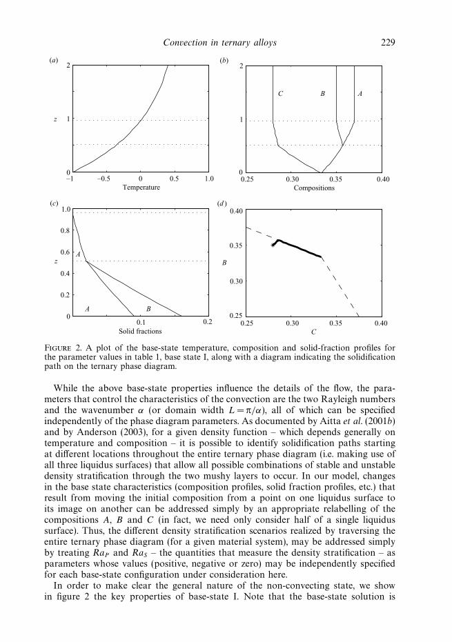
Figure 2. A plot of the base-state temperature, composition and solid-fraction profiles forthe parameter values in table 1, base state I, along with a diagram indicating the solidificationpath on the ternary phase diagram.
While the above base-state properties influence the details of the flow, the para-meters that control the characteristics of the convection are the two Rayleigh numbersand the wavenumber α (or domain width L = π/α), all of which can be specifiedindependently of the phase diagram parameters. As documented by Aitta et al. (2001b)and by Anderson (2003), for a given density function – which depends generally ontemperature and composition – it is possible to identify solidification paths startingat different locations throughout the entire ternary phase diagram (i.e. making use ofall three liquidus surfaces) that allow all possible combinations of stable and unstabledensity stratification through the two mushy layers to occur. In our model, changesin the base state characteristics (composition profiles, solid fraction profiles, etc.) thatresult from moving the initial composition from a point on one liquidus surface toits image on another can be addressed simply by an appropriate relabelling of thecompositions A, B and C (in fact, we need only consider half of a single liquidussurface). Thus, the different density stratification scenarios realized by traversing theentire ternary phase diagram (for a given material system), may be addressed simplyby treating RaP and RaS – the quantities that measure the density stratification – asparameters whose values (positive, negative or zero) may be independently specifiedfor each base-state configuration under consideration here.
In order to make clear the general nature of the non-convecting state, we showin figure 2 the key properties of base-state I. Note that the base-state solution is
230 D. M. Anderson and T. P. Schulze
0 1 2 3 4 5 6
10
20
30
40
50
60
70
80
90
100
α
Ray
leig
h nu
mbe
r
RaS = RaP
RaS = 0
RaP = 0
Figure 3. This figure shows neutral stability curves for base state I. The neutral curvefor convection with equal Rayleigh numbers (RaS = RaP ) has critical Rayleigh numbersRaP = RaS =18.04 and wavenumber α = 1.52. The neutral curve for convection driven fromthe primary mushy layer (RaS = 0) has critical Rayleigh number RaP = 23.24 and wavenumberα = 1.50. The neutral curve for convection driven from the secondary mushy layer (RaP =0)has critical Rayleigh number RaS = 64.19 and wavenumber α = 2.08.
independent of all Rayleigh numbers and the wavelength. Figure 2(a) shows that thetemperature is continuous and differentiable throughout the entire domain, owingto our simplifying assumptions of zero latent heat and equal thermal properties forall three components in both the liquid and solid phases. The dotted lines indicatethe interface positions. The composition profiles, shown in figure 2(b) are constantin the liquid and have an exponential form in the mushy layers with discontinuousderivatives at the interfaces. The fact that A= B at the secondary interface andA= B = C at the eutectic front are the result of the symmetry of the system wehave chosen to examine. Note that the composition values sum to unity along anyhorizontal line. The solid fraction profiles are shown in figure 2(c). The solid portionof the primary mushy layer consists only of material A, while the secondary mushylayer has solid material of type A and B. The curves in the secondary layer show thefraction of the solid that is material A and the total solid fraction. Thus, the fractionof material B is accounted for by the region between the curves, marked with theletter B. Finally, figure 2(d) indicates the path that the state of a representative controlvolume follows on the phase diagram as we move from the inlet conditions, markedwith the star, down to the eutectic front. This path reflects the tie-line, liquidus andcotectic constraints. As indicated in table 1, base states II and III use different initialcompositions and therefore differ from base state I primarily with respect to themaximum solid fraction and the thickness associated with each mushy layer.
The neutral stability curves shown in figure 3 correspond to base state I for the threecases of convection driven equally from both layers (RaP = RaS), from the primary
Convection in ternary alloys 231
layer only (with RaS = 0) and from the secondary layer only (with RaP = 0). All threeneutral stability curves exhibit a single-mode (i.e. local minimum) structure. In fact,all other cases investigated (including II and III, but also many other base, stateconfigurations corresponding to different initial compositions in the ternary phasediagram) displayed only unimodal neutral curves. The unimodal characteristic of theneutral stability curve has been observed for the binary alloy mushy-layer systemcalculated by Worster (1992) for the case of zero solute diffusivity and, owing to ourassumption of negligible solute diffusivity, is consistent with our observations.
The minimum Rayleigh number(s) and linear critical wavenumber can vary broadly.We have compiled this information in table 2 along with results from our nonlinearstudy, in which we were able to, in some cases, obtain independent estimates for thelinear critical Rayleigh numbers. (The nonlinear data is missing in cases where thecritical Rayleigh numbers were especially large or one of the layers was especiallythin as, these conditions lead to numerical difficulties.) Following Beckermann et al.(2000), we introduce at this point two rescaled Rayleigh numbers that characterizemore naturally the properties of each particular layer. In particular, each new Rayleigh
number has the form Ranat =(�ρ/ρ0)gΠh/(κν) so that each is based on the density
difference �ρ, thickness h and effective permeability Π for each layer (rather thanreference values of these quantities that are less representative of each particularmushy layer). After some manipulations, these new Rayleigh numbers can be relatedto those defined above by
RanatP = RaP [−T S(hP − hS)ΠP ], (5.1)
RanatS = RaS[(T
S + 1)hSΠS], (5.2)
where ΠP and ΠS are dimensionless effective permeability values for each layer.For simplicity, we have defined ΠP and ΠS as χ 3
P and χ 3S; that is the cube of the
average liquid fraction in each layer. The values of these rescaled Rayleigh numbersat the linear critical point are less variable from case to case compared to the originalversions and thus provide a more unifying basis for predicting the onset of convection.
Table 2 is organized as follows. For each base state (I, II, III) we show five con-vective scenarios: (i) RaS < 0, RaP > 0 – a very stably stratified secondary layerwith an unstably stratified primary layer; (ii) RaS = 0, RaP > 0 – a neutrally stratifiedsecondary layer with an unstably stratified primary layer; (iii) RaS = RaP – twounstably stratified mushy layers; (iv) RaS > 0, RaP = 0 – an unstably stratifiedsecondary layer with a neutrally stratified primary layer; and (v) RaS > 0, RaP < 0 –an unstably stratified secondary layer with a very stably stratified primary layer.For each case, we have given the linear critical Rayleigh numbers and wavenumbercalculated from the linear stability analysis and, where possible, the correspondinglinear critical Rayleigh numbers calculated using the nonlinear code. Table 2 alsogives further details about the bifurcating solutions, which we discuss in more detailbelow.
We point out the following general features of the results in table 2. First, the linearcritical Rayleigh number varies broadly for the different base states and convectivescenarios considered. The critical wavenumber tends to be larger for cases in whichan unstable layer is paired with a stable layer; this is generally accompanied by alocalization of the convection within the unstable layer. The largest wavenumberswere always observed in connection with convection isolated in the secondary mushylayer. In the case in which an opposing density stratification is not present, theconvection tends to be of larger scale.
232
D.M
.A
nderso
nand
T.P.Sch
ulze
Linear Nonlinear Inclusion
RaP RaS RanatP Ranat
S αc RaP RaS Bifurcation RaP RaS Amplitude Location
Table 2. Results of linear and nonlinear calculations associated with five convection scenarios for the three different base state configurations I,II and III identified in table 1. In particular, the linear critical Rayleigh numbers (for two different sets of scalings) and the critical wavenumberare shown in the five columns under the linear heading. Under the nonlinear heading, where possible, we show the two Rayleigh numbers at zeroamplitude to be compared with the corresponding ones from the linear analysis. We also indicate whether the bifurcation is supercritical (super.)or subcritical (sub.). Additionally, under the ‘Inclusion’ heading, we give the Rayleigh number values and amplitude (measured by the L2 normof the buoyancy-driven streamfunction) at which an inclusion forms. The final column indicates whether the inclusion forms as a liquid inclusion inthe primary layer (P) or as a primary mushy layer inclusion in the secondary layer (S). For the calculation of the different Rayleigh numbers underthe linear heading we note that RaP = gP Ranat
P and RaS = gSRanatS (base case I: gP = 0.1524, gS = 0.2510; base case II: gP = 0.2305, gS = 0.0282;
base case III: gP =0.0111, gS = 0.1986). For simplicity, we have defined ΠP and ΠS as χ3P and χ3
S ; that is the cube of the average liquid fractionin each layer.
Convection in ternary alloys 233
–15 –10 –5 0 5 10 15 20 25
–15
–10
–5
0
5
Stable
RaSnat
Rapnat
Unstable
0 2 4 6
1
2
0 2 4 6
1
2
0 2 4 6
1
2
0 2 4 6
1
2
Figure 4. The main solid curve corresponds to the linear critical value of the Rayleighnumbers separating stable and unstable solutions for base case I using Da = 0.05. The dashedcurve is the same result but with Da = 10−5. Insets show the convection pattern at thefour open circles along the main solid curve – moving from upper left to lower right. Theleftmost diamond shows the approximate location of the transition point from one roll (onthe right-hand side) to two stacked rolls (on the left-hand side). The rightmost diamond showsthe approximate location of the transition from one roll (on the left-hand side) to two stackedrolls (on the right-hand side).
These trends can be observed in figures 4–6, where we map out in the (RanatS , Ranat
P )-plane, an overall boundary between linearly stable and unstable regions. Figure 4shows such results for base case I using the results of the linear stability analysisdescribed in § 3. The solid curve in the main plot corresponds to the linear critical valueof the Rayleigh numbers separating stable and unstable solutions using Da = 0.05.The four inset plots show the convective streamlines at parameter values indicatedby the four open circles along the main solid curve – moving from upper left tolower right – and correspond to four of the five flow configurations detailed intable 2 (the convective pattern for the case with RaP = RaS is very similar to the caseRaP > 0, RaS = 0 and so is not shown here). In these insets, the horizontal dashedlines show interface positions separating the liquid layer, primary mushy layer andsecondary mushy layer. In the upper left inset plot, where the secondary layer isvery stably stratified, we see that the main convective flow occurs in the primarymushy layer and liquid layer. The solid horizontal line appearing in the secondarymushy layer is a separating streamline below which there is a very weak reverseflow. Comparing the four inset plots from left to right shows the convective floweventually becoming localized in the secondary mushy layer. In the lower right inset,a small-scale convection pattern appears in the secondary layer. In this case, there isa weak reverse flow occurring in the primary layer (above the horizontal separating
234 D. M. Anderson and T. P. Schulze
0 5 10 15 20 25 30 35
–300
–250
–200
–150
–100
–50
0
Unstable
Stable
RaPnat
RaSnat
2 4 60
1
20 2 4 6
1
22 4 60
1
2
2 4 60
1
2
Figure 5. The main solid curve corresponds to the linear critical value of the Rayleighnumbers separating stable and unstable solutions for base case II using Da = 0.05. Inset plotsshow the buoyant convection at the four open circles – moving from upper left to lower right –indicated on the main plot. The leftmost diamond shows the approximate location of thetransition point from one roll (on the right-hand side) to two stacked rolls (on the left-handside). The middle diamond shows the approximate location of the transition from one roll (onthe left-hand side) to two stacked rolls (on the right-hand side). The rightmost diamond showsthe approximate location of the transition from two stacked rolls (on the left-hand side) tothree stacked rolls (on the right-hand side).
streamline). We discuss these reverse flows and their impact on the solid fractiondistribution in the mushy layers in the context of the nonlinear solutions below. Thetwo open diamonds shown on the main solid curve indicate the points along the curvewhere the convective flow pattern makes a transition from single-cell flows to thesestacked-cell flows. In particular, the leftmost diamond shows the approximate locationof the transition point from one roll (on the right-hand side) to two stacked rolls (onthe left-hand side). The rightmost diamond shows the approximate location of thetransition from one roll (on the left) to two stacked rolls (on the right). Physically,the stacked cell case suggests that the main flow avoids the stably stratified region(whether it be in the primary or secondary mushy layer) where the resistance toconvective flow is large and instead prefers a configuration in which a weak reverseflow is generated in the stably stratified region.
In figure 4, the dashed curve in the main plot shows the same result as the mainsolid curve, but with a much smaller value of the Darcy number Da = 10−5 that ismore representative of physical systems than Da = 0.05. We observe a destabilizationof the flow (smaller Rayleigh numbers) primarily for the flow configurations in whichthere is significant flow in the primary mushy layer and liquid layer. Since the Darcynumber enters our calculations only in the interfacial condition at the liquid–primarymush interface, the effect of changing Da becomes negligible for convection modeslocalized in the secondary mushy layer. Corresponding to the upper left-hand portion
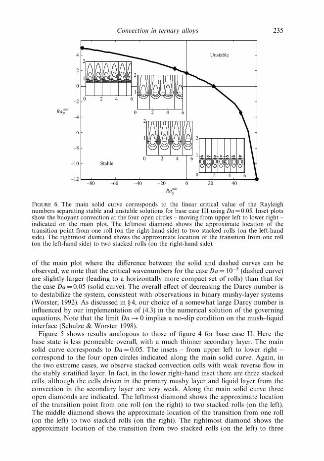
Convection in ternary alloys 235
–80 –60 –40 –20 0 20 40–12
–10
–8
–6
–4
–2
0
2
4 Unstable
Stable
2 4 60
1
2
0 2 4 6
1
2
0 2 4 6
1
2
0 2 4 6
1
2
RaPnat
RaSnat
Figure 6. The main solid curve corresponds to the linear critical value of the Rayleighnumbers separating stable and unstable solutions for base case III using Da = 0.05. Inset plotsshow the buoyant convection at the four open circles – moving from upper left to lower right –indicated on the main plot. The leftmost diamond shows the approximate location of thetransition point from one roll (on the right-hand side) to two stacked rolls (on the left-handside). The rightmost diamond shows the approximate location of the transition from one roll(on the left-hand side) to two stacked rolls (on the right-hand side).
of the main plot where the difference between the solid and dashed curves can beobserved, we note that the critical wavenumbers for the case Da = 10−5 (dashed curve)are slightly larger (leading to a horizontally more compact set of rolls) than that forthe case Da = 0.05 (solid curve). The overall effect of decreasing the Darcy number isto destabilize the system, consistent with observations in binary mushy-layer systems(Worster, 1992). As discussed in § 4, our choice of a somewhat large Darcy number isinfluenced by our implementation of (4.3) in the numerical solution of the governingequations. Note that the limit Da → 0 implies a no-slip condition on the mush–liquidinterface (Schulze & Worster 1998).
Figure 5 shows results analogous to those of figure 4 for base case II. Here thebase state is less permeable overall, with a much thinner secondary layer. The mainsolid curve corresponds to Da = 0.05. The insets – from upper left to lower right –correspond to the four open circles indicated along the main solid curve. Again, inthe two extreme cases, we observe stacked convection cells with weak reverse flow inthe stably stratified layer. In fact, in the lower right-hand inset there are three stackedcells, although the cells driven in the primary mushy layer and liquid layer from theconvection in the secondary layer are very weak. Along the main solid curve threeopen diamonds are indicated. The leftmost diamond shows the approximate locationof the transition point from one roll (on the right) to two stacked rolls (on the left).The middle diamond shows the approximate location of the transition from one roll(on the left) to two stacked rolls (on the right). The rightmost diamond shows theapproximate location of the transition from two stacked rolls (on the left) to three
236 D. M. Anderson and T. P. Schulze
stacked rolls (on the right). Finally, we again note the general trend of increasingwavenumber (decreasing wavelength) for the convection driven from the secondarylayer.
Figure 6 shows results analogous to those of figure 4 for base case III. Here, thebase state has a much thicker secondary layer (with much lower permeability) and amuch thinner primary mushy layer compared to base case I. The main solid curvecorresponds to Da =0.05. The insets – from upper left to lower right – correspondto the four open circles indicated along the main solid curve. In the upper left-handinset, the convection is driven from a very thin primary mushy layer. The main flow isconfined to the primary and liquid layers, while a very weak reverse flow occurs in therelatively impermeable secondary layer. In the lower right-hand inset, the reverse flow,driven from the secondary layer, is centred around the primary mushy layer–liquidlayer interface. On the main solid curve, the leftmost diamond shows the approximatelocation of the transition point from one roll (on the right) to two stacked rolls (onthe left) and the rightmost diamond shows the approximate location of the transitionfrom one roll (on the left) to two stacked rolls (on the right).
Before discussing the nonlinear results we comment on the validation of both thelinear and nonlinear codes used in this paper. First, the base-state solutions givenexplicitly in § 3,.1 have been reproduced to a very high degree of accuracy using thenonlinear numerical methods described in § 4. Secondly, the neutral stability curvescalculated as described in § 3 were consistently reproduced to within a few per centusing nonlinear solutions which maintained a fixed small amplitude while varying thedomain width (see linear critical Rayleigh numbers given in table 2). The differencewas attributable to the truncation error in the nonlinear code owing to a relativelycoarse grid. Thirdly, both the linear and nonlinear codes used here have been validatedby comparison with the previously computed binary results of Worster (1992) andSchulze & Worster (1999).
The computation of nonlinear finite-amplitude convecting solutions allows us toprobe further into the interaction between the convective motion set up initiallyby the density stratification and the evolution (dissolution and/or growth) of thesolid fraction in each layer. As a representative case, we shall show the nonlinearcounterparts of the four convective scenarios highlighted for base case I in the insetsof figure 4. For these nonlinear computations we fix the domain width in each caseto a value that corresponds to the linear critical wavenumber (that is, L = π/αc). Theamplitude of the flow is then increased in each case until the solid fraction (eitherφA in the primary layer or φB in the secondary layer) is driven to zero at somepoint along the centre of the cell where the downward flow is the weakest and thebuoyancy-driven portion of the flow is directly upward. We find that such inclusionscan occur either in the primary layer (in which case a liquid inclusion is formed) or inthe secondary layer (in which case we observe a primary mushy-layer inclusion). Thisinformation is also included in table 2, the last five columns of which indicate thetype of bifurcation, the values of the Rayleigh numbers and flow amplitude (norm ofthe buoyancy-driven streamfunction) and the location of the inclusion when it firstforms upon increasing the amplitude.
Figure 7 shows the nonlinear flow for base case I(i) in which the secondary mushylayer is very stably stratified and the primary mushy layer is unstably stratified. Inboth plots, the two dark solid lines indicate the position of the interfaces separatingthe liquid layer, the primary mushy layer and the secondary mushy layer. Theseinterface positions are notably perturbed from the linear stability case in which theyare planar. In Figure 7(a) we show isotherms (dashed curves) and the buoyancy-driven
Convection in ternary alloys 237
–2 –1 0 1 20
1
2(a)
(b)
–2 –1 0 1 20
1
2
Figure 7. Nonlinear solutions for base case I(i). (a) Streamlines associated with the buoyantconvection (solid curves using equal spacing of 0.1 between contours) and isotherms (dashedcurves using equal spacing of 0.25 between contours). (b) Streamlines for the total mass flux(solid curves) and the total solid fraction (dashed curves using equal spacing of 0.02 betweencontours). The diamond shows the location of a liquid inclusion in the primary mushy layer.
streamlines (solid curves). Consistent with the upper left-hand inset plot in figure 4, wesee that there is a separating streamline in the secondary layer below which a reverseflow occurs. Since this flow is very weak, these weak secondary rolls do not appearin the plot (for clarity in the main convective rolls, we have chosen equally spacedstreamline values). In figure 7(b), we show the total solid fraction contours (dashedcurves) and streamlines for the total mass flux, which has the streamfunction ψ + x
(solid curves entering at the top of the plot and exiting at the bottom). In the case ofno buoyant convection, these streamlines would be undeflected vertical lines. Alongthe centreline in the primary mushy layer is shown a region of reverse circulation and,as indicated by the diamond, the location of a liquid inclusion in the primary mushylayer. As pointed out by Schulze & Worster (1999), such a liquid inclusion must occurat the bottom of the reverse circulation streamline. This observation provides anotheruseful diagnostic for the nonlinear code. We note that the nonlinear calculations arenot designed to compute the physically valid solution beyond the amplitude at whichthe inclusion forms and so we have taken care to capture the solution as close to theinitial formation of the inclusion as possible.
Results for the other three nonlinear cases are shown in figures 8–10. In thesequence of figures for the nonlinear case, we have used the same isotherm contours,the same streamline values and the same solid fraction contours so that a morequantitative comparison can be made between the results. In particular, we can seethat the convective flow becomes progressively weaker as the flow makes a transition
238 D. M. Anderson and T. P. Schulze
–2 –1 0 1 20
1
2(a)
(b)
–2 –1 0 1 20
1
2
Figure 8. Nonlinear solutions for base case I(ii). (a) Streamlines associated with the buoyantconvection (solid curves using equal spacing of 0.1 between contours) and isotherms (dashedcurves using equal spacing of 0.25 between contours). (b) Streamlines for the total mass flux(solid curves) and the total solid fraction (dashed curves using equal spacing of 0.02 betweencontours). The diamond shows the location of a liquid inclusion in the primary mushy layer.
from being driven in the primary layer to being driven in the secondary layer. Acomparison between figures 7 and 8 shows that the two cases are very similar, withthe exception that the case with a very stably stratified secondary mushy layer hasa weak reverse flow in the secondary mushy layer (figure 7) rather than a relativelydeep penetration of the main flow into the secondary layer (figure 8). In both of thesecases, a liquid inclusion forms in the primary mushy layer along the centreline. Forthe two flows driven from the secondary mushy layer, as shown in figures 9 and 10,we observe the formation of a primary mushy layer inclusion in the secondary mushylayer. For the case of a very stably stratified primary mushy layer, we note that thereis again a weak reverse flow in the primary mushy layer corresponding to a stackedconvective roll (figure 10). While the solid fraction contours in this case are depressedalong the centreline in the secondary mushy layer (indicative of chimney formationwhere there is a strong upflow) they are very slightly elevated along the centreline inthe primary mushy layer (where there is a downflow due to the reversed convectioncells). Finally, we note that the deflection of the interface positions from horizontalbecomes less pronounced for the cases in which the flow is driven from the secondarymushy layer. This is due to the overall relatively weak flow that occurs in these cases.
6. ConclusionIn this paper, we have adopted the model of ternary alloy solidification first
analysed by Anderson (2003) in the context of diffusion-controlled growth from afixed boundary and have applied it to study convective effects during directional
Convection in ternary alloys 239
–1.5 –1.0 –0.5 0 0.5 1.0 1.50
1
2(a)
(b)
–1.5 –1.0 –0.5 0 0.5 1.0 1.50
1
2
Figure 9. Nonlinear solutions for base case I(iv). (a) Streamlines associated with the buoyantconvection (solid curves using equal spacing of 0.1 between contours) and isotherms (dashedcurves using equal spacing of 0.25 between contours). (b) Streamlines for the total mass flux(solid curves) and the total solid fraction (dashed curves using equal spacing of 0.02 betweencontours). The diamond shows the location of a primary mush inclusion in the secondarymushy layer.
solidification at a steady rate V . We have performed a linear stability analysis of thissystem and have computed strongly nonlinear convective steady states that developfrom the initial bifurcation. To this end, we have reduced the parameter set by acombination of scaling and simplifying assumptions to focus exclusively on the roleof convection.
Before discussing our results in more detail, we emphasize two general conclusionsconcerning convection in ternary mushy zones. First, we found that the role ofconvection could be characterized by two Rayleigh numbers – one for each mushylayer – that combine all of the effects on the local density induced by changes inspecies compositions and the thermal environment. This generalizes the binary case(see Worster 1997) where the mushy layer can be characterized by a single Rayleighnumber. Secondly, we found that, the tie-line constraint, (2.11), can be generalizedto situations with fluid flow. As noted earlier, this condition is a consequence ofnegligible solutal diffusivity and the uniform inlet concentrations that result in theentire primary layer being constrained to the same tie-line.
Convection in the ternary alloy system is controlled first by the two independentRayleigh numbers, but is also influenced by the base state properties such as mushy-layer thickness and permeability. The overall depth of the combined mushy layers isdependent primarily on the far-field temperature, while the relative thickness of eachlayer, as well as the permeability of each layer, is controlled mainly by the initialliquid compositions. An array of different base-state configurations were examined.
240 D. M. Anderson and T. P. Schulze
–0.6 –0.4 –0.2 0 0.2 0.4 0.60
1
2
–0.6 –0.4 –0.2 0 0.2 0.4 0.60
1
2(b)
(a)
Figure 10. Nonlinear solutions for base case I(v). (a) Streamlines associated with the buoyantconvection (solid curves using equal spacing of 0.1 between contours) and isotherms (dashedcurves using equal spacing of 0.25 between contours). (b) Streamlines for the total mass flux(solid curves) and the total solid fraction (dashed curves using equal spacing of 0.02 betweencontours). The diamond shows the location of a primary mush inclusion in the secondarymushy layer.
For representative base states, our linear and nonlinear results documented convectionin the ternary alloy system for cases in which: (i) the secondary layer was very stablystratified and the primary layer was unstably stratified, (ii) the secondary layer wasneutrally stratified and the primary layer was unstably stratified, (iii) both layers wereunstably stratified, (iv) the secondary layer was unstably stratified and the primarylayer was neutrally stratified, and (v) the secondary layer was unstably stratified andthe primary layer was very stably stratified.
The penetration of convection from an unstably stratified layer to a stably stratifiedlayer was controlled by the strength and location of the unstable stratification andthe permeability contrast between layers. Convection in the primary layer was foundto generally induce a flow (comparable in magnitude) in the liquid layer, but only aweak flow in the secondary layer. This was particularly notable if the secondary layerhad a much lower permeability. Convection in the secondary mushy layer, however,generally produced a significant flow in the primary and liquid layers unless theprimary layer (which always had a higher average permeability than the secondarylayer) was sufficiently stably stratified to effectively contain the convection within thesecondary layer.
We found that a sharp stability contrast between primary and secondary layersleads to smaller-scale convection (in our calculations the smallest scale patterns werealways associated with convection confined to a secondary layer by a very stablystratified primary mushy layer). It was in these cases where we observed ‘stacked’convection cells. That is, with convection primarily localized in the unstable layer,
Convection in ternary alloys 241
there was an adjacent set of rolls circulating in the opposite direction in the stablystratified layer. These stacked rolls were observed consistently in the linear solutionsand the nonlinear solutions. Here we found that along a vertical line through bothmushy layers, the solid fraction perturbation could be negative in one region andpositive in another.
Our nonlinear calculations were consistent with our linear results, but also showedthe further development of the flow at finite amplitude. As with its binary alloycounterpart, the ternary mushy-layer system is composed of reactive porous mediawhose solid matrix may undergo growth or dissolution as a result of transport of heatand solute by the flow. We have identified two manifestations of this property. First,for convection driven in the primary mushy layer, we found that nonlinear stateswith liquid inclusions in the primary mushy layer were possible. These inclusionsare similar to those identified by Schulze & Worster (1999) for binary alloys. Forconvection driven in the secondary layer, we found that nonlinear states with primarymushy-layer inclusions in the secondary mushy layer (which is composed of dendritesof one species as well as dendrites of a second species) were possible.
While convection was found to be the result of a nearly vertical bifurcation overthe range of amplitudes where the solid fractions remained positive, the nonlinearcalculations revealed that the bifurcation for convection driven in the primary mushylayer was supercritical, and that driven in the secondary mushy layer was subcritical.Since the inclusion first develops where convection is the strongest, liquid inclusions inthe primary layer were associated with supercritical bifurcations and mush inclusionsin the secondary layer were associated with subcritical bifurcations. While this wastrue of all the cases we examined, including some not presented here, we emphasizethat this correlation may not hold generally. This would be an interesting topic toexplore with a weakly nonlinear analysis, which would allow for a computationallymore efficient exploration of parameter space. A nonlinear stability analysis wouldalso confirm that the subcritical solutions are unstable and the supercritical solutionsstable, which is what we would anticipate from other convection problems. If thisis indeed the case, the inclusions that form along a supercritical bifurcation couldbe studied experimentally – an option that is apparently unavailable for the binarysystem.
There are several additional avenues that warrant further investigation. First, thereis the issue of modelling and calculating solutions with inclusions of primary mushin the secondary layer. This is a phenomenon unique to the ternary case and may besomewhat easier to capture than the liquid inclusions characteristic of the binary casesince the governing equations are virtually the same on both sides of the interface.This situation would require a further generalization of the tie-line constraint so thateach streamline entering such an inclusion would carry its own composition ratiofor the passive species. Secondly, the inclusion of solutal diffusion (where the tie-lineconstraint does not apply) may reveal new convective modes not observed here. Inparticular, we anticipate that the inclusion of solutal diffusivity in the ternary casewill lead to a second mode of fine-scale convection in the diffusive boundary layerat the liquid–mush interface analogous to that identified for binary convection byWorster (1992). In the ternary alloy, Anderson (2003) showed the existence of asolute boundary layer above the mush–mush interface and we may expect additionalmodes associated with this boundary layer. Finally, a detailed analysis of the effectsof thermal convection in the ternary system, as was undertaken for binary alloys byChen et al. (1994), as well as the effects of time dependence and three-dimensionalgeometry may be both tractable and of interest for ternary alloys.
242 D. M. Anderson and T. P. Schulze
The authors would like to acknowledge support from the 3M Non-Tenured FacultyAward Program (D.M.A.) and the National Science Foundation, DMS–0306996(D.M.A.) and DMS–0405650 (T.P.S.). The authors would also like to thank G. B.McFadden and M. G. Worster for helpful discussions.
REFERENCES
Aitta, A., Huppert, H. E. & Worster, M. G. 2001a Diffusion-controlled solidification of a ternarymelt from a cooled boundary. J. Fluid Mech. 432, 201–217.
Aitta, A., Huppert, H. E. & Worster, M. G. 2001b Solidification in ternary systems. In InteractiveDynamics of Convection and Solidification (ed. P. Ehrhard, D. S. Riley & P. H. Steen),pp. 113–122. Kluwer.
Amberg, G. & Homsy, G. M. 1993 Nonlinear analysis of buoyant convection in binary solidificationwith application to channel formation. J. Fluid Mech. 252, 79–98.
Anderson, D. M. 2003 A model for diffusion-controlled solidification of ternary alloys in mushylayers. J. Fluid Mech. 483, 165–197.
Anderson, D. M. & Worster, M. G. 1995 Weakly nonlinear analysis of convection in mushy layersduring the solidification of binary alloys J. Fluid Mech. 302, 307–331.
Anderson, D. M. & Worster, M. G. 1996 A new oscillatory instability in a mushy layer duringthe solidification of binary alloys. J. Fluid Mech. 307, 245–267.
Beckermann, C., Gu, J. P. & Boettinger, W. J. 2000 Development of a freckle predictor via Rayleighnumber method for single-crystal nickel-base superalloy castings. Metall. Mat. Trans. A 312545–2557.
Bloomfield, L. J. & Huppert, H. E. 2003 Solidification and convection of a ternary solution cooledfrom the side. J. Fluid Mech. 489, 269–299.
Boettinger, W. J., Kattner, U. R., Coriell, S. R., Chang, Y. A. & Mueller, B. A. 1995Development of multicomponent solidification micromodels using a thermodynamic phasediagram data base. In Modeling of Casting, Welding and Advanced Solidification Process VII(ed. M. Cross & J. Campbell) pp. 649–656. Warrendale, PA.
Chen, F., Lu, J. W. & Yang, T. L. 1994 Convective instability in ammonium chloride solutiondirectionally solidified from below. J. Fluid Mech. 276, 163–187.
Chung, C. A. & Chen, F. 2000 Onset of plume convection in musy layers. J. Fluid Mech. 408,53–82.
Chung, C. A. & Worster, M. G. 2002 Steady-state chimneys in a mushy layer. J. Fluid Mech. 455,387–411.
Davis, S. H. 2001 Theory of Solidification. Cambridge University Press.
Emms, P. W. & Fowler, A. C. 1994 Compositional convection in the solidification of binary alloys.J. Fluid Mech. 262, 111–139.
Felicelli, S. D, Poirier, D. R. & Heinrich, J. C. 1997 Macrosegregation patterns inmulticomponent Ni-base alloys. J. Cryst. Growth 177, 145–161.
Felicelli, S. D, Poirier, D. R. & Heinrich, J. C. 1998 Modeling freckle formation in threedimensions during solidification of multicomponent alloys. Metall. Mat. Trans. B 29, 847–855.
Krane, M. J. M. & Incropera, F. P. 1997 Solidification of ternary metal alloys–II. Prediction ofconvective phenomena and solidification behaviour of Pb–Sb–Sn alloys. Intl J. Heat MassTransfer 40, 3837–3847.
Krane, M. J. M., Incropera, F. P. & Gaskell, D. R. 1997 Solidification of ternary metal alloys–I.Model development. Intl J. Heat Mass Transfer 40, 3827–3835.
Krane, M. J. M., Incropera, F. P. & Gaskell, D. R. 1998 Solidification of a ternary metal alloy:a comparison of experimental measurements and model predictions in a Pb–Sb–Sn system.Metall. Mat. Trans. A 29, 843–853.
McKibbin, R. & O’Sullivan, M. J. 1980 Onset of convection in a layered porous medium heatedfrom below. J. Fluid Mech. 96, 375–393.
McKibbin, R. & O’Sullivan, M.J. 1981 Heat transfer in a layered porous medium heated frombelow. J. Fluid Mech. 111, 141–173.
Nield, D. A & Bejan, A. 1999 Convection in Porous Media, 2nd. edn. Springer.
Convection in ternary alloys 243
Riahi, D. N. 2002 On nonlinear convection in mushy layers. Part 1. Oscillatory modes of convection.J. Fluid Mech. 467, 331–359.
Schneider M. C., Gu, J. P., Beckermann, C., Boettinger, W. J. & Kattner, U. R. 1997 Modelingof micro- and macrosegregation and freckle formation in single-crystal nickel-base superalloydirectional solidification. Metall. Mat. Trans. A 28, 1517–1531.
Schulze, T. P. & Worster, M. G. 1998 A numerical investigation of steady convection in mushylayers during the directional solidification of binary alloys. J. Fluid Mech. 356, 199–220.
Schulze, T. P. & Worster, M. G. 1999 Weak convection, liquid inclusions and the formation ofchimneys in mushy layers. J. Fluid Mech. 388, 197–215.
Schulze, T. P. & Worster, M. G. 2001 Mushy zones with fully developed chimneys. In InteractiveDynamics of Convection and Solidification (ed. P. Ehrhard, D. S. Riley & P. H. Steen),pp. 71–80. Kluwer.
Schulze, T. P. & Worster, M. G. 2005 A time-dependent formulation of the mushy-zone-freeboundary problem. J. Fluid Mech. 541, 193–202.
Smallman, R. E. 1985 Modern Physical Metallurgy. Butterworths.
Thompson, A. F., Huppert, H. E. & Worster, M. G. 2003a A global conservation model fordiffusion-controlled solidification of a ternary alloy. J. Fluid Mech. 483, 191–197.
Thompson, A. F., Huppert, H. E., Worster, M. G. & Aitta, A. 2003b Solidification andcompositional convection of a ternary alloy. J. Fluid Mech. 497, 167–199.
Trefethen, L. N. 2000 Spectral Methods in Matlab. SIAM, Philadelphia.
Worster, M. G. 1986 Solidification of an alloy from a cooled boundary. J. Fluid Mech. 167, 481–501.
Worster, M. G. 1992 Instabilities of the liquid and mushy regions during solidification of alloys.J. Fluid Mech. 237, 649–669.
Worster, M. G. 1997 Convection in mushy layers. Annu. Rev. Fluid Mech. 29, 91–122.
Worster, M. G. 2000 Solidification of Fluids. In Perspectives in Fluid Dynamics (ed. G. K. Batchelor,H. K. Moffatt & M. G. Worster), pp. 393–446. Cambridge University Press.