MIT OpenCourseWare http://ocw.mit.edu

18.01 Single Variable Calculus Fall 2006

For information about citing these materials or our Terms of Use, visit: http://ocw.mit.edu/terms.

����

Lecture 9 18.01 Fall 2006

Lecture 9: Linear and Quadratic Approximations

Unit 2: Applications of Differentiation

Today, we’ll be using differentiation to make approximations.

Linear Approximation

y=f(x)

y = b+a(x-x0)y

x

b = f(x0) ;

x0 ,f(x0)( )

a = f’(x0 )

Figure 1: Tangent as a linear approximation to a curve

The tangent line approximates f(x). It gives a good approximation near the tangent point x0. As you move away from x0, however, the approximation grows less accurate.

f(x) ≈ f(x0) + f �(x0)(x − x0)

Example 1. f(x) = ln x, x0 = 1 (basepoint)

1 f(1) = ln 1 = 0; f �(1) = = 1

x x=1

ln x

Change the basepoint:

Basepoint u0 = x0 − 1 = 0.

≈ f(1) + f �(1)(x − 1) = 0 + 1 · (x − 1) = x − 1

x = 1 + u = ⇒ u = x − 1

ln(1 + u) ≈ u

1

Basic list of linear approximations

In this list, we always use base point x0 = 0 and assume that |x| << 1.

1. sin x ≈ x (if x ≈ 0) (see part a of Fig. 2)

2. cos x ≈ 1 (if x ≈ 0) (see part b of Fig. 2) x3. e ≈ 1 + x (if x ≈ 0)

4. ln(1 + x) ≈ x (if x ≈ 0)

5. (1 + x)r ≈ 1 + rx (if x ≈ 0)

Proofs

Proof of 1: Take f(x) = sin x, then f �(x) = cos x and f(0) = 0

f �(0) = 1, f(x) ≈ f(0) + f �(0)(x − 0) = 0 + 1.x

So using basepoint x0 = 0, f(x) = x. (The proofs of 2, 3 are similar. We already proved 4 above.)

Proof of 5:

f(x) = (1 + x)r; f(0) = 1

f �(0) = d

(1 + x)rx=0 = r(1 + x)r−1

x=0 = rdx

| |

f(x) = f(0) + f �(0)x = 1 + rx

y = x

sin(x)

y=1

cos(x)

(a) (b)

Figure 2: Linear approximation to (a) sin x (on left) and (b) cos x (on right). To find them, apply f (x) ≈ f (x0) + f �(x0)(x − x0) (x0 = 0)

e−2x

Example 2. Find the linear approximation of f(x) = near x = 0. √1 + x

We could calculate f �(x) and find f �(0). But instead, we will do this by combining basic approxi­mations algebraically.

u e−2x ≈ 1 + (−2x) (e ≈ 1 + u, where u = −2x)

2

Lecture 9 18.01 Fall 2006

√1 + x = (1 + x)1/2 ≈ 1 +

1 x

2 Put these two approximations together to get

e−2x 1 − 2x

x ≈ (1 − 2x)(1 +

1 x)−1√

1 + x ≈

1 + 1 22

Moreover (1 + 1 x)−1 ≈ 1 − 1 x (using (1 + u)−1 ≈ 1 − u with u = x/2). Thus 1 2 2

e−2x 1 1 1 2√1 + x

≈ (1 − 2x)(1 − 2 x) = 1 − 2x −

2 x + 2(

2)x

Now, we discard that last x2 term, because we’ve already thrown out a number of other x2 (and higher order) terms in making these approximations. Remember, we’re assuming that x << 1.

2 3 | |

This means that x is very small, x is even smaller, etc. We can ignore these higher-order terms, because they are very, very small. This yields

e−2x 1 5 √1 + x

≈ 1 − 2x − 2 x = 1 −

2 x

Because f(x) ≈ 1 − 5 x, we can deduce f(0) = 1 and f �(0) =

−5 directly from our linear approxi­

2 2 mation, which is quicker in this case than calculating f �(x).

Example 3. f(x) = (1 + 2x)10 .

On the first exam, you were asked to calculate lim (1 + 2x)10 − 1

. The quickest way to do this with x→0 x

the tools of Unit 1 is as follows.

lim (1 + 2x)10 − 1

= lim f(x) − f(0)

= f �(0) = 20 x 0 x x 0 x→ →

(since f �(x) = 10(1 + 2x)9 2 = 20 at x = 0) ·

Now we can do the same problem a different way, namely, using linear approximation.

(1 + 2x)10 ≈ 1 + 10(2x) (Use (1 + u)r ≈ 1 + ru where u = 2x and r = 10.)

Hence, (1 + 2x)10 − 1 1 + 20x − 1

= 20 x

≈ x

Example 4: Planet Quirk Let’s say I am on Planet Quirk, and that a satellite is whizzing overhead with a velocity v. We want to find the time dilation (a concept from special relativity) that the clock onboard the satellite experiences relative to my wristwatch. We borrow the following equation from special relativity:

T T � = �

1 − vc2

2

1 1 11A shortcut to the two-step process √1 + x

≈ 1 + x ≈ 1 −

2 x is to write

2

1 1 √

1 + x = (1 + x)−1/2 ≈ 1 −

2 x

3

Lecture 9 18.01 Fall 2006

me

satellite

(with velocity v)

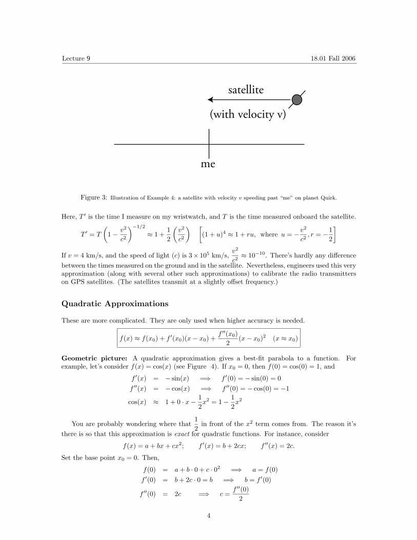
Figure 3: Illustration of Example 4: a satellite with velocity v speeding past “me” on planet Quirk.

Here, T � is the time I measure on my wristwatch, and T is the time measured onboard the satellite. � 2 �−1/2 �

2 � � 2 �

v 1 v v 1 T � = T 1 −

c2 ≈ 1 +

2 c2 (1 + u)4 ≈ 1 + ru, where u = −

c2 , r = −

2 2

If v = 4 km/s, and the speed of light (c) is 3 × 105 km/s, v ≈ 10−10 . There’s hardly any difference c2

between the times measured on the ground and in the satellite. Nevertheless, engineers used this very approximation (along with several other such approximations) to calibrate the radio transmitters on GPS satellites. (The satellites transmit at a slightly offset frequency.)

Quadratic Approximations

These are more complicated. They are only used when higher accuracy is needed.

f(x) ≈ f(x0) + f �(x0)(x − x0) + f ��(x0) (x − x0)2 (x ≈ x0)2

Geometric picture: A quadratic approximation gives a best-fit parabola to a function. For example, let’s consider f(x) = cos(x) (see Figure 4). If x0 = 0, then f(0) = cos(0) = 1, and

f �(x) = − sin(x) = ⇒ f �(0) = − sin(0) = 0

f ��(x) = − cos(x) = ⇒ f ��(0) = − cos(0) = −1 1 1

cos(x) ≈ 1 + 0 · x − 2 x 2 = 1 −

2 x 2

1You are probably wondering where that in front of the x2 term comes from. The reason it’s

2 there is so that this approximation is exact for quadratic functions. For instance, consider

f(x) = a + bx + cx 2; f �(x) = b + 2cx; f ��(x) = 2c.

Set the base point x0 = 0. Then,

f(0) = a + b 0 + c 02 = a = f(0)· · ⇒

f �(0) = b + 2c 0 = b = b = f �(0)· ⇒

f ��(0)f ��(0) = 2c = c = ⇒

2

4

Lecture 9 18.01 Fall 2006

cos(x)

y

x

1- x2/2

Figure 4: Quadratic approximation to cos(x).

0.0.1 Basic Quadratic Approximations

:

f(x) ≈ f(0) + f �(0)x + f ��

2(0)

x 2 (x ≈ 0)

1. sin x ≈ x (if x ≈ 0)

2x2. cos x ≈ 1 −

2 (if x ≈ 0)

3. e x ≈ 1

1 + x + x 2 (if x ≈ 0)2

4. ln(1 + x) ≈ x − 1 x 2 (if x ≈ 0)

2

5. (1 + x)r ≈ 1 + rx + r(r − 1)

x 2 (if x ≈ 0)2

Proofs: The proof of these is to evaluate f(0), f �(0), f ��(0) in each case. We carry out Case 4

⇒f(x) = ln(1 + x) = f(0) = ln 1 = 01

f �(x) = [ln(1 + x)]� = = f �(0) = 11 + x

⇒ � �1

f ��(x) = 1 +

� −1 x

= (1 + x)2

= ⇒ f ��(0) = −1

Let us apply a quadratic approximation to our Planet Quirk example and see where it gives. �

1 − v

c2

2 �−1/2

≈ 1 + 21 v

c2

2

+

� ( −2

1 )( −

2 21 − 1)

�

− v

c2

2 �2 �

Case 5 with x = −c

v2

2

, r = − 21

5

Lecture 9 18.01 Fall 2006

� �22 2

Since v ≈ 10−10, that last term will be of the order

v ≈ 10−20 . Not even the best atomic c2 c2

clocks can measure time with this level of precision. Since the quadratic term is so small, we might as well ignore it and stick to the linear approximation in this case.

e−2x

Example 5. f(x) = √1 + x

Let us find the quadratic approximation of this expression. We can rewrite it as f(x) = e−2x(1 + x)−1/2 . Using the approximation of each factor gives �

1 � �

1 �

(− 12 )(− 12 − 1) �

2

�

f(x) ≈ 1 − 2x + 2(−2x)2 1 −

2 x +

2 x

1 1 2 +3 5 27 2f(x) ≈ 1 − 2x −

2x + (−2)(−

2)x 2 + 2x

8 x 2 = 1 −

2 x +

8 x

(Note: we drop the x3 and higher order terms. This is a quadratic approximation, so we don’t care about anything higher than x2.)

6

Lecture 9 18.01 Fall 2006