Linear Control Toolbox - supporting B-splines in LPV control☆,☆☆
Maarten Verbandt⁎, Laurens Jacobs, Dora Turk, Taranjitsingh Singh, Jan Swevers,Goele PipeleersMECO Research Team, Department of Mechanical Engineering, KU Leuven; DMMS lab, Flanders Make, Leuven, Belgium
A R T I C L E I N F O
Keywords:Linear Control ToolboxMatlabLPVB-splineModelingIdentificationControl
A B S T R A C T
This paper presents the Linear Control Toolbox, a freely available Matlab-based software package primarilyfocused on optimal feedback controller design for LTI and LPV systems. Its main goal is to make more involvedcontroller design methodologies accessible to the broader public by providing tailored synthesis and analysistools. The paper gives an overview of the different modules within the toolbox, the underlying data structuresand the supported functionalities and algorithms. Moreover two case studies are elaborated. The autopilot of amissile serves as a comparison of the Linear Control Toolbox with its competitors and an overhead crane setupwas used to demonstrate the use and experimentally validate the presented toolbox.
1. Introduction
Since the early days of control theH∞/H2 framework has received alot of attention. It reformulates the LTI controller design as an opti-mization problem where the objectives and constraints are based onH∞ and/orH2 norms of closed-loop transfer functions. As a result, oneis guaranteed to obtain the optimal stabilizing controller given a par-ticular set of constraints. Also robustness requirements fit naturally inthis framework. All these aspects combined make the H∞/H2 frame-work very appealing.
An additional advantage of the H∞/H2 framework is that it natu-rally extends to Linear Parameter Varying control. The LPV paradigmholds the middle ground between the restricted class of LTI systems onthe one hand and the general class of nonlinear systems on the other:while being able to capture particular nonlinear phenomena, LPVcontrol is supported by a similar wealth of analysis and design tools asLTI control. Moreover, LPV control has been widely validated in aca-demia, supporting its practical value [1]. However, the absence of fa-cilitating software tools seems to be the impeding factor to get LPVcontrol adopted by industry. For LPV H∞/H2 control, the need fordedicated software is even more emergent than for LTI. In comparisonto the LTI case, optimization based LPV control faces the additionalchallenge of satisfying the constraints over the entire parameter do-main. Various methods have been designed to handle this problem, but
still a substantial effort is needed to transform the controller design intoa tractable optimization problem. Some steps in the direction of user-friendly software have been made though. Matlab’s Robust ControlToolbox supports LPV controller design in a very general fashion that ismainly based on the work of Apkarian and co-workers [2,3]. So-calledtunableSurface objects capture a general parameter dependencyand are used to parameterize and design an LPV controller. In case theparameter dependency is affine, the user can resort to the more con-venient hinfgs. LPVtools, as described by Hjartarson et al. [4], isanother Matlab-based package which is intended to ease the manip-ulation with, analysis of and design for both gridded and parameterizedLPV systems. Within LPVtools a polynomial parameter dependency isemployed.
This paper focuses on a new Linear Control Toolbox,1 which is anextension to Verbandt [5]. The motivation is twofold. The main driveris to support recent developments in LPV controller design, based on B-splines as described by Hilhorst et al. [6]. This method allows para-meter dependencies to be described by B-splines which are more flex-ible than the traditionally employed polynomials. Since B-splines en-compass polynomials, traditional analysis and design methods can stillbe interfaced with this new toolbox. Second existing tools are primarilyfocused on control, tailored to a specific LPV design problem. Thisforces the user to switch toolboxes to for instance identify an LPVsystem or to design an LTI controller. On the contrary, the Linear
https://doi.org/10.1016/j.mechatronics.2018.04.007Received 23 November 2017; Received in revised form 13 April 2018; Accepted 25 April 2018
☆ This work benefits from KU Leuven-BOF PFV/10/002 Centre of Excellence: Optimization in Engineering (OPTEC); the Belgian Programme on Interuniversity Attraction Poles,initiated by the Belgian Federal Science Policy Office (DYSCO); Flanders Make project ROCSIS: Robust and Optimal Control of Systems of Interacting Subsystems; and project G091514Nof the Research Foundation-Flanders (FWO-Flanders). Flanders Make is the Flemish strategic research center for the manufactoring industry.
☆☆ This paper was recommended for publication by Associate Editor Dr Oomen Tom.⁎ Corresponding author.E-mail address: [email protected] (M. Verbandt).
1 The Linear Control Toolbox can be found at https://github.com/meco-group/lc_toolbox.
Control Toolbox supports the control engineer throughout the differentsteps involved in controller design both in an LTI and an LPV setting. Itprovides the functionality to identify a system, facilitates general ma-nipulations with systems, enables the user to declare a control config-uration and a list of specifications, automatically solves the optimalcontroller design problem and provides frequency and time domainvalidation tools.
The remainder of the paper is structured as follows. The first partfocuses on the internal system modeling module, which handles generalsystem manipulations. Next, the identification module is touched upon,followed by a detailed explanation of the controller design module. Inaddition, two case studies are provided. The first is concerned with thedesign of a missile’s autopilot and compares the Linear Control Toolboxto LPVtools and the Robust Control Toolbox. The second exampleconsiders an overhead crane with varying cable length for which anLPV controller is designed and experimentally validated. The paperends with some concluding remarks.
2. System modeling module
At the core of the presented toolbox resides a general systemmodeling module. This module adopts a new design paradigm whichmakes a clear distinction between systems and models. A system re-flects a physical entity, e.g. a pump, an electrical circuit or a chemicalprocess. All of these have inputs and outputs which are intrinsicallyrelated. This relationship is never truly known but one or more modelsof the same system might be available. Therefore a system can be re-garded as a collection of models which all refer to the same physicalentity. The advantage of this approach is that different models can beconsulted when most relevant. For instance, the controller design mightbe based on a simplified linear model whereas a time-domain simula-tion of a high-fidelity nonlinear model is preferable for a validation.Using a custom modeling module also gives the opportunity to in-troduce new model classes such as a general nonlinear model, a gridded(LPV) model or a parameter dependent state-space model.
The following paragraphs shed a brighter light on the toolbox’sunderstanding of systems and signals, models and parameters, and theirmutual relation.
2.1. Systems and signals
Within the Linear Control Toolbox, systems and signals serve thepurpose of describing a configuration, i.e. how different componentsinteract with each other. Systems are created via the function call
> G = IOSystem(ni,no)where ni and no denote the number of inputs and outputs. Inputs
and outputs are internally stored as a Signal and can be accessed via:> G.in, G.outThe user is also encouraged to use signal aliases which make the
code easier to read:> u = G.in, y = G.outMoreover, new signals can be constructed either via the Signal()
call or as a linear combination of other signals, for example:
> r = Signal(n)> e = r - y
where the optional argument n indicates the dimension of the signal.Signals serve the purpose of connecting systems together. A connectionis established by simply equating the signals with the = = operator andcreating a new system from the subsystems and the connection list:
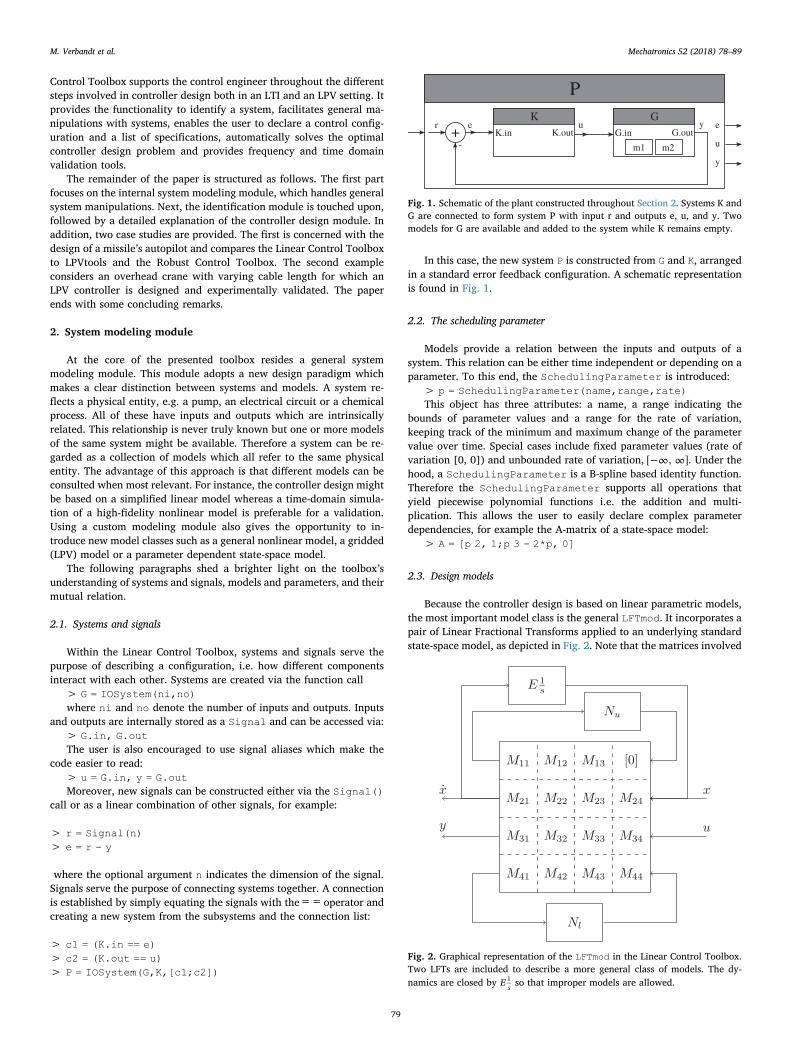
In this case, the new system P is constructed from G and K, arrangedin a standard error feedback configuration. A schematic representationis found in Fig. 1.
2.2. The scheduling parameter
Models provide a relation between the inputs and outputs of asystem. This relation can be either time independent or depending on aparameter. To this end, the SchedulingParameter is introduced:
> p = SchedulingParameter(name,range,rate)This object has three attributes: a name, a range indicating the
bounds of parameter values and a range for the rate of variation,keeping track of the minimum and maximum change of the parametervalue over time. Special cases include fixed parameter values (rate ofvariation [0, 0]) and unbounded rate of variation, −∞ ∞[ , ]. Under thehood, a SchedulingParameter is a B-spline based identity function.Therefore the SchedulingParameter supports all operations thatyield piecewise polynomial functions i.e. the addition and multi-plication. This allows the user to easily declare complex parameterdependencies, for example the A-matrix of a state-space model:
> A = [p 2, 1;p 3 - 2*p, 0]
2.3. Design models
Because the controller design is based on linear parametric models,the most important model class is the general LFTmod. It incorporates apair of Linear Fractional Transforms applied to an underlying standardstate-space model, as depicted in Fig. 2. Note that the matrices involved
Fig. 1. Schematic of the plant constructed throughout Section 2. Systems K andG are connected to form system P with input r and outputs e, u, and y. Twomodels for G are available and added to the system while K remains empty.
Fig. 2. Graphical representation of the LFTmod in the Linear Control Toolbox.Two LFTs are included to describe a more general class of models. The dy-namics are closed by E s
1 so that improper models are allowed.
M. Verbandt et al. Mechatronics 52 (2018) 78–89
79
need not be constant, allowing linear parameter varying (LPV) models.The resulting state and output dynamics are given by:
= − = −− −F N I M N F N I M N( ) , ( )u u u l l l111
441
A corresponding constructor is provided as:> mlft = LFTmod(M,Nu,Nl,E,p,Ts)where M is a 4-by-4 cell-array and Nu, Nl and E are matrices of
corresponding sizes. It is readily seen that providing empty feedbackmatrices Nu and Nl reduces the LFTmod to a standard descriptor state-space model. The latter is made directly available via the call:
> mdss = DSSmod(A,B,C,D,E,p,Ts)where A, B, C, D and E are standard state-space matrices, Ts denotes
the sample time in seconds and p is the scheduling parameter which isonly required if one or more state-space matrices depend on p. In case Ehappens to be the unit matrix, the DSSmod further reduces to a standardstate-space model which is constructed straightaway as:
> mss = SSmod(A,B,C,D,p,Ts)Although the implementation relying heavily on the LFTmod might
look over-complicated, there are two advantages in doing so. First, morecomplex operations such as closing a loop become very simple on modelsin the LFT form [7]. Second, the LFTmod is able to represent the complexmodel structures which arise naturally from an LPV controller design [8].
2.4. Validation models
For validation purposes, the toolbox provides more dedicated modelclasses such as nonlinear models or nonparametric models like a sam-pled frequency response.
To capture arbitrary nonlinear dynamics, e.g. to perform a timedomain validation, the ODEmod is introduced. This model incorporatesa general ordinary differential equation (ODE) which is driven by u andp, i.e. the input to the system and the parameter value. The state x isupdated via Eq. (1). Note that x might be empty, e.g. for a saturationblock. Eq. (2) returns the output, y, of the model.
=E x u p x f x u p( , , ) ˙ ( , , ) (1)
=y g x u p( , , ) (2)
An ODEmod is constructed by:> mode = ODEmod(f,g,E,p)where f, g and E are function handles with two or three inputs,
depending on whether a scheduling parameter is involved. In case thesefunction handles do depend on a scheduling parameter, the latter is alsorequired as an input argument of the model.
The presented toolbox also offers the possibility to work with non-parametric FRFs. The FRDmod class is built on top of Matlab’s frd class,transferring all original functionality:
> mfrd = FRDmod(resp,freq)The Gridmod represents a gridded implementation of an LPV
model. Take for instance a series of local identification experimentswhich each yield an FRDmod linked to a particular parameter value.These are readily combined in a Gridmod via the function call:
The main advantage is that all operations performed on theGridmod are carried out on all underlying elements at once, e.g.computing an element-wise norm or plotting a series of Bode diagrams.
2.5. Adding models to systems
Once one or more models have been created, they should be linkedto the corresponding system. To do so, the function add is used:
> G.add(mss,mode,mfrd)Thereafter, G.content() is no longer empty. Though standard
plotting functionality like bode or step is supported for individualmodels, calling these functions on systems is more powerful. This showsall responses on a single graph, facilitating the comparison betweendifferent (closed-loop) models.
3. System identification
The system identification module provides the necessary function-ality to convert measured time or frequency domain data into para-metric models. It interfaces the Matlab implementations [9] of thefrequency domain system identification methods in detail elaborated in[10].
Although the focus currently lies on LTI identification, LPV identi-fication is planned to be incorporated in the near future. In particularthe combined global and local LPV system identification approach [11],as well as the reweighted ℓ2, 1-norm regularization approach [12] willbe supported. In the meantime, LPV models are identified via the State-space Model Interpolation of Local Estimates (SMILE) [13], a techniquethat interpolates LTI models with a user-specified set of basis functionsof the scheduling parameter. B-spline basis functions are used here inorder to comply with the B-spline based LPV controller design withinthe toolbox.
3.1. Excitation signals and measurement data
The first step of the system identification procedure is the genera-tion of excitation signals. At present, the toolbox only supports thegeneration of multisine signals [10]. The command
creates a multisine, sampled at 100 Hz, exciting a linearly spacedfrequency grid in the interval [0.01, 2] Hz, with a frequency resolutionof 0.01 Hz. This choice automatically determines the period of themultisine, in this case 100 s. The multisine u is a so-called TimeSignalobject that contains all information that is characteristic for this specificsignal. Additional name-value pairs allow the user to specify moreoptions, e.g. the phase distribution of the signal, its amplitude spec-trum, etc. TimeSignal objects feature useful methods; the user can forexample plot the signal spectrum by
> plotSpectrum(u, ‘dft’)
The actual signal content (one period of the multisine in this case) isobtained by
> [s,t] = signal(u)
Once the excitation has been applied, the experimental data is im-ported in the toolbox. This is done by wrapping the measurements intoTDMeasurementData objects. In case of a system with two inputs andtwo outputs, a TDMeasurementData object is constructed as follows:
where u1 and u2 are objects of the aforementioned class TimeSignalrepresenting the first and the second input. Similar to TimeSignal, thetoolbox supports several relevant operations on TDMeasurementDataobjects. For example, to avoid the effect of transients in the FRF esti-mation (Section 3.2), one may decide to keep the last 7 periods of themeasurements:
> meas1 = clip(meas1, ‘lastnper’, 7)
Complementary to TDMeasurementData, theFDMeasurementData class handles nonparametric frequency re-sponse function (FRF) measurements. FRF measurements can either beloaded directly into Matlab or can be calculated based on time domaindata from a TDMeasurementData object. The latter is discussed in thefollowing paragraph.
3.2. Nonparametric frequency response function estimation
The toolbox supports two methods to estimate the system’s FRFbased on multiple measurements obtained with different random mul-tisine realizations: the robust detection algorithm for nonlinearities [10,Section 4.3.1] (Robust_NL_Anal [9]) intended for SISO systems andthe robust local polynomial method [10, Section 7.2.2] (RobustLo-calPolyAnal [9]) for MIMO systems. These methods combine mea-surements from different random multisine excitations to average outboth the effects of nonlinear distortions and measurement noise. Theyyield an FRF estimate, also referred to as the best linear approximation,the sample total variance (contributions of measurement noise andnonlinear distortions) and the sample noise variance.
The nonparametric FRF estimate based on e.g. four different mea-surements is obtained by calling the routine nonpar_ident with thearguments as shown below:
where ‘x1’, ‘x2’, ‘y1’ and ‘y2’ refer to the datalabels provided tothe TDMeasurementData objects. The result, FRF, is aFDMeasurementData object.
3.3. Parametric LTI model identification
The nonparametric FRF of the system is further used to estimate aparametric model. For the time being, the toolbox comes with theroutine MIMO_ML, a maximum likelihood identification algorithm [10],MIMO_NLS, a nonlinear least-squares fitting algorithm allowing an ar-bitrary frequency weighting weight, and also interfaces Matlab’sroutine tfest. These methods estimate common denominator transferfunction models. The function param_ident parses the data for eachof these routines and is called as shown below:
> model = param_ident(‘data’, FRF, ‘method’,‘MIMO_NLS’, “settings’, settings)
where denh (numh) and denl (numl) in settings represent thehighest and lowest degree of the denominator (numerator) of the un-derlying transfer functions, respectively. numh and numl are no× nimatrices, with no and ni the number of system outputs and inputs, re-spectively.
3.4. LTI state-space model interpolation
To obtain an LPV model the aforementioned procedure is repeatedfor different fixed values of the scheduling parameter yielding a set ofparametric LTI models. Subsequently, an LPV state-space model is ob-tained in two steps. First, the identified LTI models are packed in aGridmod:
> mgrd = Gridmod(models,schGrid)
where models is a cell array of local LTI models and schGrid is theset of corresponding values of the scheduling parameter.
Second, an LPV state-space model is obtained from the griddedmodel through an interpolation carried out by the SMILE technique[13] and a user defined basis:
Since one of the goals of the presented toolbox is to facilitate thedesign of optimal controllers, another key module is the controllerdesign module. The H∞/H2 design paradigm is introduced first, fol-lowed by the formulation and the solution of a standard control pro-blem using the toolbox.
4.1. The H∞/H2 paradigm
The idea behind the H∞/H2 paradigm [14] is to formulate thecontroller design procedure as an optimization problem. Objectives andconstraints are imposed directly on the closed-loop transfer functionsby means of H∞ and/or H2 norms. By doing so, one is guaranteed toobtain the optimal stabilizing controller given a particular set of con-straints. Moreover, it is well known that standard objectives and con-straints such as bandwidth, robustness or noise suppression can beexpressed readily within this framework.
Eq. (3)displays the standardH∞/H2 optimization problem.Ci andCjdenote the closed-loop transfer functions of interest in the objectiverespectively the constraints. Frequency dependent weights [15]W ,i V ,iWj and Vj are usually added to balance the importance of differentfrequencies. pi and pj indicate which system norm is used for eachchannel and can either be 2 of∞. αi allows a trade-off between multipleobjectives.
WCV
W C V
∑
⩽
αminimize
subject to 1K i
i i i i p
j j j p
i
j (3)
Most solvers reformulate optimization problem (3) in terms of linearmatrix inequalities (LMIs) [16]. By choosing a single Lyapunov matrixwhich applies to all of the considered channels, it is possible to renderthe design problem convex. This yields an efficient solution strategywhich naturally extends to the design of LPV controllers. In that case,the LMIs become parameter dependent and have to be relaxed to obtaina tractable formulation. Traditionally Pólya’s method [17] or Sum-of-Squares [18] are employed, but more recently it has been shown that B-spline relaxations outperform these methods in many cases [6]. It isshown that the parameter dependent LMIs are guaranteed to hold overthe whole parameter domain by putting constraints on the coefficientsFi, of the basis functions B ,i as described by Eq. (4).
B∑= ≺ ∀ ∈ ⇐ ≺=
F p p F p P F( ) ( ) 0, 0i
N
i i i1 (4)
Moreover, B-splines are capable of describing non-hyperrectangularparameter domains. The aforementioned reasons encouraged the use of
M. Verbandt et al. Mechatronics 52 (2018) 78–89
81
B-splines to capture parameter dependencies and to solve the LPV op-timal controller design problem.
4.2. Channels, norms and weights
Though optimization problem (3) might still be comprehensible to acontrol practitioner, the actual implementation is not. Two main diffi-culties arise. First, the control engineer has to choose a solver im-plementation which fits the problem at hand. This task is not obvious asit depends on several criteria, for instance: Does the problem involvehard constraints? Is the problem formulated withH∞ norms only? Is theproblem single- or multi-objective? The second hurdle is providing theright arguments to the routine. Not only do these arguments vary fromroutine to routine, but also the construction of the usually requiredaugmented plant itself might cause problems.
In order to simplify the problem formulation, the Linear ControlToolbox offers the Channel and Norm classes. A Channel is an ab-stract representation of a transfer function with input in and outputout and is constructed as:
> C = Channel(in,out,name)Multidimensional in and out are allowed, yielding a MIMO
channel.The second ingredient is the so-called weighting function. Although
weighting functions can in principle be any transfer function, they oftenboil down to standard filters. Therefore, the presented toolbox offersthe Weight class which implements these standards. Moreover, in theSISO case, the inverse of the weights can be regarded as upper boundsto the closed-loop transfer functions. Therefore Weight employs aninverse definition allowing the user to interpret the specified transferfunctions as constraints for the optimization rather than frequencydependent weights for the closed-loop transfer functions. The simplestpossible weight is a constant, constraining the peak of a transfer func-tion:
> W = Weight.DC(value)Since control engineers typically prefer a logarithmic scale, value
is by default interpreted in [dB]. In case value is to be interpreted as is,the argument ‘linear’ should be supplied. Due to the inverse defi-nition, the actual magnitude of W will be -value [dB].
> W = Weight.LF(fco,ord,lfgain)puts emphasis on lower frequencies and is therefore suited to shape
a sensitivity transfer function. At low frequencies, its magnitude ap-proaches -lfgain [dB]. ord poles are inserted so that the cross-overfrequency becomes fco. Again, natural parameters are employed toshape the weight. Its counterpart Weight.HF also exists, amplifyinghigh frequencies which is for instance applicable to ensure noise sup-pression.
In combination with a weighting function, the Channel yields aNorm object. The latter is then used to formulate the optimizationproblem in a natural way (cfr. Eq. (3)). A Norm is readily constructedvia:
> N = Norm(W,C,p)where W and C are the weight and channel respectively. In this case
the output of C is weighted by W. To have weighted inputs which isespecially relevant in a MIMO setting, the arguments W and C areswapped. The third argument p specifies which norm is being employedand can take two values: 2 or inf. In case p is omitted, the default infis employed. In that case, the shorthand notation
> N = W*Cis also available.
4.3. Obtaining a solution
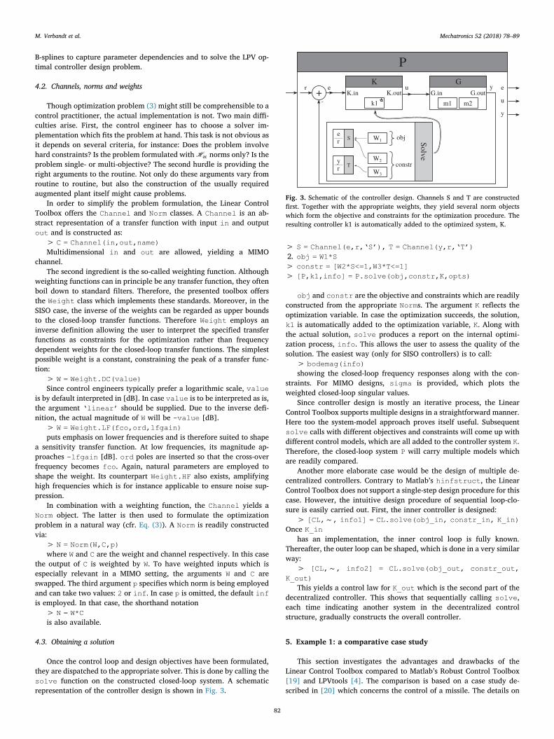
Once the control loop and design objectives have been formulated,they are dispatched to the appropriate solver. This is done by calling thesolve function on the constructed closed-loop system. A schematicrepresentation of the controller design is shown in Fig. 3.
> S = Channel(e,r,‘S’), T = Channel(y,r,‘T’)2. obj = W1*S> constr = [W2*S<=1,W3*T<=1]> [P,k1,info] = P.solve(obj,constr,K,opts)
obj and constr are the objective and constraints which are readilyconstructed from the appropriate Norms. The argument K reflects theoptimization variable. In case the optimization succeeds, the solution,k1 is automatically added to the optimization variable, K. Along withthe actual solution, solve produces a report on the internal optimi-zation process, info. This allows the user to assess the quality of thesolution. The easiest way (only for SISO controllers) is to call:
> bodemag(info)showing the closed-loop frequency responses along with the con-
straints. For MIMO designs, sigma is provided, which plots theweighted closed-loop singular values.
Since controller design is mostly an iterative process, the LinearControl Toolbox supports multiple designs in a straightforward manner.Here too the system-model approach proves itself useful. Subsequentsolve calls with different objectives and constraints will come up withdifferent control models, which are all added to the controller system K.Therefore, the closed-loop system P will carry multiple models whichare readily compared.
Another more elaborate case would be the design of multiple de-centralized controllers. Contrary to Matlab’s hinfstruct, the LinearControl Toolbox does not support a single-step design procedure for thiscase. However, the intuitive design procedure of sequential loop-clo-sure is easily carried out. First, the inner controller is designed:
This yields a control law for K_out which is the second part of thedecentralized controller. This shows that sequentially calling solve,each time indicating another system in the decentralized controlstructure, gradually constructs the overall controller.
5. Example 1: a comparative case study
This section investigates the advantages and drawbacks of theLinear Control Toolbox compared to Matlab’s Robust Control Toolbox[19] and LPVtools [4]. The comparison is based on a case study de-scribed in [20] which concerns the control of a missile. The details on
Fig. 3. Schematic of the controller design. Channels S and T are constructedfirst. Together with the appropriate weights, they yield several norm objectswhich form the objective and constraints for the optimization procedure. Theresulting controller k1 is automatically added to the optimized system, K.
M. Verbandt et al. Mechatronics 52 (2018) 78–89
82
the model and the design objectives are followed by a discussion on theproblem formulation in each of the toolboxes. Finally an assessment ofthe underlying methodologies for the controller synthesis is done, basedon the quality of the solution as well as the speed at which it is ob-tained.
5.1. Model and design objectives
The controlled system is chosen to be the missile model described in[20] which is described by Eq. (5). The system consists of one controlinput, δm, which represents the fin deflection. The measured outputs arethe normalized vertical acceleration, αzv, and the missile’s pitch rate, q.Moreover, the missile’s dynamics change under influence of two aero-dynamical coefficients, Zα∈ [0.5 4] and Mα∈ [0 105], which are thescheduling parameters for the LPV controller design.
⎡⎣⎢
⎤⎦⎥
=⎡⎣⎢
−−
⎤⎦⎥
⎡⎣⎢
⎤⎦⎥
+ ⎡⎣⎢
⎤⎦⎥
⎡⎣⎢
⎤⎦⎥
=⎡⎣⎢
− ⎤⎦⎥
⎡⎣⎢
⎤⎦⎥
αq
ZM
αq δ
αq
αq
˙˙
10
01
1 00 1
α
αm
zv
(5)
The control configuration is depicted in Fig. 4. The normalizedvertical acceleration’s tracking error e is fed back together with themissile’s pitch rate q. Based on these measurements, the control lawcomputes the fin deflection. The goal is to achieve accurate tracking forthe normalized vertical acceleration while taking into account robust-ness requirements. Therefore the design objective, given by (6), consistsof two parts. Adequate reference tracking is ensured by taking
→ = −S r e α r: zv into account. The second term in the objective en-courages robustness since the latter is guaranteed if ‖W2KS‖≤ 1.
∞
W SW KSminimize 1
2 (6)
with
=+
= ++ + +
Ws
W s ss e s e s e
2.010.201
9.678 0.0291.203 4 1.136 7 1.066 10
1
23 2
3 2 (7)
5.2. Constructing an LPV model
The first step in the controller design is to enter the missile’s LPVmodel in the different toolboxes (see code Example 1). LPVtools and theLinear Control Toolbox employ a very similar approach when it comesto declaring an LPV model. Each of the toolboxes provides a parameterobject: LPVtools comes with tvreal and pgrid whereas the LinearControl Toolbox offers SchedulingParameter. This approach makesit very intuitive to declare for instance a parameter varying state-spacematrix. Consequently, the resulting code resembles the model descrip-tion in (5) which is helpful to the user. Matlab’s Robust Control Toolboxemploys a very different strategy inspired by the polytopic nature of thesupported models. The vertices of the polytope are defined as a series ofLTI models which combined with a description of the parameter
domain result in a polytopic system. This approach requires more careas the order of vertices has to correspond to the list of LTI models. Also,the resulting code shows less resemblance to the model description (5)which might be perceived by the user as more challenging.
5.3. Declaring the control configuration
To proclaim the control configuration depicted in Fig. 4, each of thediscussed toolboxes provides its own signal-based method. The LinearControl Toolbox uses a syntax as discussed in Section 2.1 and distin-guishes itself from the other toolboxes by using explicit Signal objectsand IOSystem objects which carry input and output signals. LPVtoolsuses sysic as a connection front-end which is a string-based approach.The Robust Control Toolbox offers similar functionality throughsconnect, also parsing a series of strings to construct the inter-connected system. Code Example 2 shows the construction of the con-trol configuration within the different toolboxes.
Although a comparison of these different implementations dependsheavily on the user’s preferences, it is tried to make it as objective aspossible. The first criterion is the readability of the produced code. Inthat respect the Linear Control Toolbox and LPVtools would surpass theRobust Control Toolbox since the former rely on additional variables todeclare the plant. The ability to supply convenient names for the signalsalso adds to the readability of the code. This feature is present in boththe Robust Control Toolbox and the Linear Control Toolbox which inthat regard outperform LPVtools. Moreover, the Linear Control Toolboxand the Robust Control Toolbox also include the controller in the for-mulation of the control configuration which feels more natural thanconstructing an open loop to which the controller still needs to beconnected, as is the case with LPVtools. On the other hand, LPVtoolsand the Robust Control Toolbox impose a more structured declarationthan the Linear Control Toolbox which helps preventing unconnectedmodels or unresolved connections.
When it comes to expressing the control objectives, it is usuallyrequired to extend the control configuration with appropriate weightsto obtain the augmented plant. Therefore, these weights are alreadyincluded in the control configuration Paug when using LPVtools or theRobust Control Toolbox. Contrary to its alternatives, the Linear ControlToolbox provides a higher level of abstraction to formulate the opti-mization problem as described by Section 4.2. Based on this optimi-zation problem, the augmented plant is constructed behind the scenes.This allows the user to declare simply the actual control configurationrather than the augmented plant which is merely a mathematical con-struct.
Generally speaking, the Linear Control Toolbox is very much or-iented to the user’s comfort, mainly improving the readability of thecode. The Robust Control Toolbox sits at the other end of the spectrum,usually resulting in compact code intended for expert users. LPVtoolsholds the middle ground providing tools to simplify the controller de-sign to some extent.
5.4. Solving the control problem
The missile control problem is now passed to the solvers in thedifferent toolboxes in order to compare the quality of the solution aswell as the speed at which it is obtained. However, when passing theproblem to LPVtools, an error is thrown related to a rank deficient D21matrix in the augmented plant. Following the instructions provided byMegretski [21], a regularization input was added to the control con-figuration leading to a successful solution. The Linear Control Toolbox’ssolver was invoked with the var_deg = 0 resulting in a constantLyapunov matrix. LPVtools’ lpvsyn was executed with the ‘Min-Gamma’ flag to avoid a relaxation of the optimal value which wouldlead to an unfair comparison. Because LPVtools offers two parameterrepresentations, tvreal and pgrid, both solutions are presented.
The results are gathered in Table 1. In terms of optimality, the
Fig. 4. Control configuration for the vertical acceleration control of a missile.The control output δm is based on the tracking error e and the missile’s pitchrate q as an additional measurement. (adapted from [20]).
M. Verbandt et al. Mechatronics 52 (2018) 78–89
83
Linear Control Toolbox and the Robust Control Toolbox show com-parable performance whereas LPVtools lags behind with both solutionstrategies. This is also clearly visible from Fig. 5, particularly from the
sensitivity: the green and yellow curves show a lower bandwidth thanthe red and blue curves, which implies that LPVtools reaches a lowerdegree of optimality. This also shows in the step response subject to aspiral parameter trajectory (8) depicted in Fig. 6. The two controllersdesigned with LPVtools are slower than the other two responses.
The opposite holds when comparing the solver times. Here LPVtools aswell as the Robust Control Toolbox outperform the Linear ControlToolbox. Moreover the Linear Control Toolbox’s solver is an order of
Code example 1. Comparison of the Linear Control Toolbox, LPVtools and the Robust Control Toolbox when constructing the missile’s LPV model.
Code example 2. Comparison of the Linear Control Toolbox, LPVtools and the Robust Control Toolbox when constructing the control configuration.
Table 1Comparison of the optimality and solver time of the Robust Control Toolbox,LPVtools and the Linear Control Toolbox.
magnitude slower than its competitors. However the time it takes tosolve the underlying SDP is only 0.96 s which is more in line withLPVtools and the Robust Control Toolbox. The 16 s overhead is causedby the controller synthesis tools being based on the ‘OptiSpline’ toolbox[22]. This toolbox eases the manipulation of splines at the expense of anextra cost to export the underlying SPD. A direct implementation of theLMIs would put the B-spline based method amongst its competitors.
Although this case study would suggest there are only minor dif-ferences between the different toolboxes regarding the quality of thesolution, it should be noted that the case study was chosen so that alltoolboxes were able to solve the same problem. Both LPVtools and theLinear Control Toolbox are capable of solving a broader variety ofproblems than the Robust Control Toolbox. They can handle poly-nomial and B-spline parameterized models respectively and deal withconstrained parameter variations explicitly.
6. Example 2: experimental validation on an overhead crane
This section demonstrates the use of the Linear Control Toolboxwhen designing an LPV controller for an overhead crane system. Thefirst part covers the physical modeling of the system resulting in anonlinear model. This model is well suited for validation but not forcontroller design. This is why a second model is derived, based on aseries of identification experiments. These result in local LTI modelswhich are interpolated to obtain an LPV model. Based on the latter, a
parameter varying controller is designed and validated both in simu-lation and experimentally.
6.1. Modeling
A schematic of the considered mechatronic system is depicted inFig. 7. The base of the system consists of a velocity controlled trolleywith time constant τ and reference u. The encoder on the trolley’s trackprovides a measurement of x0. The trolley is equipped with a hoistingmechanism which allows the system to vary the cable length L, which isalso being measured. Moreover, L is constrained between 0.3 m and0.8 m with a maximum rate of variation of 10 cm/s. Another sensor onthe hoisting mechanism measures the load angle θ. These measure-ments are combined to obtain a measurement for the output of interest,x. Eq. (9) shows the governing dynamics, adapted from Debrouwereet al. [23]. The model parameter τ is approximately 0.01 s and thedamping coefficient c is set to 0 m/s.
⎧
⎨⎪
⎩⎪
=− −= − − −= +
−
− −
x τ x uθ L τ x u θ g θ cθx x L θ
¨ ( ˙ )¨ ( ( ˙ )cos sin ˙)
sin
01
01 1
0
0 (9)
Code example 3describes the declaration of the crane. First a SISOsystem, crane, is constructed. Next, the scheduling parameter L isintroduced followed by a declaration of the nonlinear equations ofmotion. As a last step, the nonlinear model nl is added to the systemcrane.
6.2. Identification of an LPV model
Because the previously derived nonlinear model is not suited forcontroller design, an identification experiment is set up to derive sev-eral LTI models for a set of fixed cable lengths. Code example 4 de-scribes how the toolbox creates an excitation signal and how it is ex-ported to drive the actual setup. First the experimental settings aredefined: the sample frequency fs, the number of samples of the peri-odic excitation signal N, the frequency resolution df and the range ofexcited frequencies frange (all frequencies specified in [Hz]). Basedon these settings, an excitation signal is generated. A full random phasemultisine with amplitude 0.05 m/s is opted for. This signal is thenwritten to a text file using Matlab’s dlmwrite, which in turn is fed tothe overhead crane. Once an experiment has been carried out, the datais imported in the Linear Control Toolbox. TDMeasurementData isprovided as the standard time domain data container and is constructedas described by Code example 5. First, the control value u and themeasured output y are read from the data file ‘exp_50.nc’, createdduring the experiment. Next they are packed together with the origin-ally constructed excitation signal in the TDMeasurementData object.Moreover, the signals are labeled ‘input’ and ‘loadpos’ and the data is
Fig. 5. Comparison of the closed-loop transfer functions within the three con-troller design toolboxes. (For interpretation of the references to colour in thisfigure legend, the reader is referred to the web version of this article.)
Fig. 6. Step response of the missile’s autopilot on a spiral parameter trajectory(8).
Fig. 7. Schematic of the considered overhead crane. The cart is driven by thevelocity reference u. x0, θ and L are measured.
M. Verbandt et al. Mechatronics 52 (2018) 78–89
85
marked as being periodic. In order to estimate the LTI models for dif-ferent cable lengths, a two-step approach is used. This is described byCode example 6. In the first step, the measured data is fed to non-par_ident which estimates a nonparametric FRF. The input andoutput label indicate which measurements are to be used and ‘Ro-bust_NL_anal’ indicates the employed method. Note that clip isused to only retain the last three periods of the measured responsethereby suppressing the influence of the transient on the resulting fre-quency response. The nonparametric estimates for various cable lengthsare shown on Fig. 8. It is observed that the identification results degradetowards higher frequencies. However, from a control point of view, it ismainly the resonance frequency that needs a decent estimate whichjustifies continuing with these models. The second step involves theestimation of a parametric model. To this end, param_ident is in-voked on npmod_50 using the method‘MIMO_NLS’.
The previously described sequence of creating an excitation signal,loading the measured data and estimating a model is repeated for cablelengths from 0.3 m to 0.8 m in steps of 0.05 m. The different LTI modelsare combined in one Gridmod, as it serves naturally as a sampledversion of an underlying LPV model. Given a B-spline basis and a
scheduling parameter, the gridded model is readily transformed into anLPV state-space model through interpolation. This LPV model is thenadded to the system crane. This is described in Code example 7. Fig. 8shows the bode diagrams of the different models involved: the fixed-length FRFs, the fixed-length LTI models and the varying length LPVmodel.
6.3. Controller design
Designing a controller involves two steps: proclaiming the controlconfiguration and stating the design specifications. The presentedtoolbox facilitates both by offering a suitable syntax.
First the configuration, depicted in Fig. 9, is built. The corre-sponding code is found in Code example 8. Since the system crane, hasalready been declared, the only system still needed is the controller, K.After introducing the reference signal r, aliases are provided for themeasured output of the crane, y, the control signal, u and the errorsignal, e, which improves the readability. Finally, the set of connectionsis passed on to a new system together with the subsystems involved,resulting in the desired configuration. Note that at this point, theclosed-loop transfer functions are not accessible because the controllerK does not yet contain any models.
Second, the list of specifications is provided, as shown inCode example 9. Two requirements are imposed: the controller’s highfrequency roll-off should be -20 dB per decade and the bandwidthshould be at least 0.15 Hz. The transfer functions of interest are →r eand →r u, also referred to as the sensitivity (S) and the input sensitivity(U). Roll-off is guaranteed by constraining the weighted input sensi-tivity. The weight is designed so that high frequencies become domi-nant in the H∞ criterion, effectively suppressing them. By choosing afirst order weight, the requirement of high frequency controller roll-offis met. Similarly, the sensitivity’s low frequencies are amplified by Ws inorder to obtain better tracking behavior. The cross-over frequency of Wsis chosen 0.15 Hz to satisfy the design requirement. The remaining
Code example 3. Declaration of the crane system and construction of the nonlinear model.
Code example 4. Code necessary to generate and export a multisine excitationsignal for the overhead crane setup.
Code example 5. Code necessary to generate and export a multisine excitation signal for the overhead crane setup.
M. Verbandt et al. Mechatronics 52 (2018) 78–89
86
freedom is used to maximize the damping of the closed loop, i.e. pe-nalizing Ms*S. By calling solve on the closed loop P, along with thedesign specifications, the optimal controller is computed and auto-matically added to system K.
6.4. Validation
The Linear Control Toolbox also offers some validation tools, al-lowing the user to critically assess the design.
Because the controller design was based on anH∞ criterion, one cancheck how the closed-loop transfer functions relate to the imposedconstraints. By simply calling bodemag(sol,S,U,T), the closed-looptransfer functions are shown along the with weights, as depicted inFig. 10. It is clearly visible that all constraints are met: the closed-loop
Code example 6. Estimation of a fixed-length LTI models for the overhead crane.
Code example 7. Interpolation of local LTI models to obtain an LPV model.
Fig. 8. Bode diagram of the different models involved in the identificationprocess. In blue the estimated nonparametric FRF for fixed cable lengths, ingreen the corresponding LTI models and in red the evaluation of the inter-polated LPV model at the corresponding cable lengths. The B-spline’s four de-grees of freedom are used to optimally interpolate the 11 local LTI models. (Forinterpretation of the references to colour in this figure legend, the reader isreferred to the web version of this article.)
Fig. 9. Schematic of the control configuration of the overhead crane.
Code example 8. Declaration of the control configuration in the Linear ControlToolbox.
Code example 9. Stating the design specifications and computing the optimalcontroller.
M. Verbandt et al. Mechatronics 52 (2018) 78–89
87
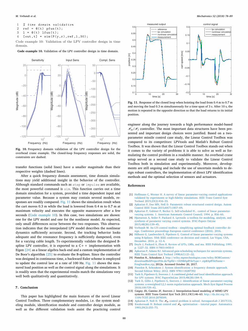
transfer functions (solid lines) have a smaller magnitude than theirrespective weights (dashed lines).
After a quick frequency domain assessment, time domain simula-tions may yield additional insight in the behavior of the controller.Although standard commands such as step or impulse are available,the most powerful command is sim. This function carries out a timedomain simulation for a system, provided a time dependent input andparameter value. Because a system may contain several models, re-sponses are readily compared. Fig. 11 shows the simulation result whenthe cart moves 0.3 m while the load is lowered from 0.4 m to 0.7 m atmaximum velocity and executes the opposite manoeuvre after a fewseconds (Code example 10). In this case, two simulations are shown:one for the LPV model and one for the nonlinear model. As expected,only small differences occur between the two responses. This observa-tion indicates that the interpolated LPV model describes the nonlineardynamics sufficiently accurate. Second, the tracking behavior looksadequate and the resonance frequency is sufficiently dampened, evenfor a varying cable length. To experimentally validate the designed B-spline LPV controller, it is exported to a C++ implementation withEigen [24] as a linear algebra back-end and a custom implementation ofDe Boor’s algorithm [25] to evaluate the B-splines. Since the controllerwas designed in continuous time, a backward Euler scheme is employedto update the control law at a rate of 100 Hz. Fig. 11 shows the mea-sured load position as well as the control signal along the simulations. Itis readily seen that the experimental results match the simulations verywell both qualitatively and quantitatively.
7. Conclusion
This paper has highlighted the main features of the novel LinearControl Toolbox. Three complementary modules, i.e. the system mod-eling module, identification module and controller design module, aswell as the different validation tools assist the practicing control
engineer along the journey towards a high performance model-basedH∞/H2 controller. The most important data structures have been pre-sented and important design choices were justified. Based on a two-parameter missile control case study, the Linear Control Toolbox wascompared to its competitors: LPVtools and Matlab’s Robust ControlToolbox. It was shown that the Linear Control Toolbox stands out whenit comes to the variety of problems it is able to solve as well as for-mulating the control problem in a readable manner. An overhead cranesetup served as a second case study to validate the Linear ControlToolbox both in simulation and experimentally. Moreover, develop-ments are still ongoing and include the use of uncertain models to de-sign robust controllers, the implementation of direct LPV identificationmethods and the optimal selection of sensors and actuators.
References
[1] Hoffmann C, Werner H. A survey of linear parameter-varying control applicationsvalidated by experiments or high-fidelity simulations. IEEE Trans Control SystTechnol 2015;23(2):416–33.
[2] Apkarian P, Dao MN, Noll D. Parametric robust structured control design. AutomControl IEEE Trans 2015;60(7):1857–69.
[3] Apkarian P, Gahinet P, Becker G. Self-scheduled H∞ control of linear parameter-varying systems. 1. American Automatic Control Council; 1994. p. 856–60.
[4] Hjartarson A, Seiler P, Packard A. Lpvtools: a toolbox for modeling, analysis, andsynthesis of parameter varying control systems. IFAC-Papers OnLine2015;48(26):139–45.
[5] Verbandt M. An LTI control toolbox - simplifying optimal feedback controller de-sign. Conference proceedings European control conference (2016). 2016.
[6] Hilhorst G, Lambrechts E, Pipeleers G. Control of linear parameter-varying systemsusing B-Splines. 55th IEEE conference on decision and control, Las Vegas, USA,December. 2016. p. 12–4.
[7] Doyle J, Packard A, Zhou K. Review of LFTs, LMIs, and mu. IEEE Publishing; 1991.p. 1227–32. ISBN 0-7803-0450-0
[8] Apkarian P, Adams RJ. Advanced gain-scheduling techniques for uncertain systems.IEEE Trans Control Syst Technol 1998;6(1):21–32.
[9] Pintelon R., Schoukens J. http://wiley.mpstechnologies.com/wiley/BOBContent/downloadBobProjectFile.do?bpfId=1029&bpfFileType=.zip&bpfFileName=FreqDomBox.zip; 2012a. Accessed October 20, 2017.
[10] Pintelon R, Schoukens J. System identification: a frequency domain approach.Second Edition Wiley; 2012. ISBN 9781118287392
[11] Turk D, Pipeleers G, Swevers J. A combined global and local identification approachfor LPV systems. IFAC PapersOnLine 2015;48(28):184–9.
[12] Turk D, Gillis J, Pipeleers G, Swevers J. Identification of linear parameter-varyingsystems: a reweighted L2,1-norm regularization approach. Mech Syst Signal Process2018;100:729–42.
[13] Caigny JD, Camino JF, Swevers J. Interpolation-based modeling of MIMO LPVsystems. IEEE Trans Control Syst Tech 2011;19(1):46–63. http://dx.doi.org/10.1109/TCST.2010.2078509.
[14] Apkarian P, Noll D. The H∞ control problem is solved. AerospaceLab J 2017(13).[15] Kwakernaak H. Robust control and H∞ optimization – tutorial paper. Automatica
1993;29(2):255–73.
Code example 10. Validation of the LPV controller design in time domain.
Fig. 10. Frequency domain validation of the LPV controller design for theoverhead crane example. The closed-loop frequency responses are solid, theconstraints are dashed.
Fig. 11. Response of the closed loop when hoisting the load from 0.4 m to 0.7 mand moving the load 0.3 m simultaneously for a time span of 3 s. After 10 s, themotion is repeated in the opposite direction so that the load returns to its initialposition.
[16] Gahinet P, Apkarian P. A linear matrix inequality approach to H∞ control. Int JRobust Nonlinear Control 1994;4:421–48.
[17] Pólya G. Über positive darstellung von polynomen. Vierteljschr Naturforsch GesZürich 1928;73:141–5.
[18] Marshall M. Positive polynomials and sum of squares. Mathematical surveys andmonographs. American Mathematical Society; 2008.
[19] Mathworks. Robust control toolbox. https://nl.mathworks.com/products/robust.html, Accessed: 2018-03-05.
[20] Gahinet P., Nemirovski A., Laub A.J., Chilali M. LMI control toolbox; chap. 7. 1995,p. 10–14.
[21] Megretski A. Dynamic systems and control. Lecture notes (Fall 2006) WellPosedness of LTI Feedback Design; 2006. p. 9–10. Chap. 21
[22] Lambrechts E., Gillis J. Optispline. https://github.com/meco-group/optispline;2018.
[23] Debrouwere F, Vukov M, Quirynen R, Diehl M, Swevers J. Experimental validationof combined nonlinear optimal control and estimation of an overhead crane.Proceedings of the 19th IFAC world congress. 2014. p. 9617–22.
[24] Guennebaud G., Jacob B., et al. Eigen v3. http://eigen.tuxfamily.org; 2010.[25] De Boor C. A practical guide to splines. 27. Applied Mathematical Sciences; 2001.