In this paper, the inverse eigenvalue problem of reconstructing a Jacobi matrix from its eigenvalues, its leading principal submatrix and part of the eigenvalues of its submatrix is considered. The necessary and sufficient conditions for the existence and uniqueness of the solution are derived. Furthermore, a numerical algorithm and some numerical examples are given.
Arc-based integer programming formulations for three variants ofproportional symbol maps✩
Rafael G. Canoa, Cid C. de Souzaa,∗, Pedro J. de Rezendea, Tallys Yunesb
a Institute of Computing, University of Campinas, Campinas, SP 13083-852, Brazilb School of Business Administration, University of Miami, Coral Gables, FL 33124-8237, USA
h i g h l i g h t s
• A new formulation is described to create optimal proportional symbol maps.• We address three problem variants, two of which are known to be NP-hard.• Efficient separation routines and lifting procedures are described.• The new formulation is up to 82 times faster than the others in the literature.• Most known benchmark instances can now be solved in less than one minute.
a r t i c l e i n f o
Article history:Received 14 January 2014Received in revised form 12 February2015Accepted 2 September 2015
MSC:90C1090C2790C5790C9052B12
Keywords:Integer linear programmingComputational geometrySymbol mapsCartographyVisualization
a b s t r a c t
Proportional symbol maps are a cartographic tool that employs scaled symbolsto represent data associated with specific locations. The symbols we consider areopaque disks, which may be partially covered by other overlapping disks. We ad-dress the problem of creating a suitable drawing of the disks that maximizes one oftwo quality metrics: the total and the minimum visible length of disk boundaries.We study three variants of this problem, two of which are known to be NP-hardand another whose complexity is open. We propose novel integer programming for-mulations for each problem variant and test them on real-world instances with abranch-and-cut algorithm. When compared with state-of-the-art models from theliterature, our models significantly reduce computation times for most instances.
✩ Research supported by grants from Conselho Nacional de Desenvolvimento Cientıfico e Tecnologico (CNPq) #477692/2012-5,#311140/2014-9, #302804/2010-2, Fundacao de Amparo a Pesquisa do Estado de Sao Paulo (Fapesp) #2007/52015-0,#2012/00673-2.∗ Corresponding author.
Proportional symbol maps are a cartographic tool to visualize data associated with specific locations(e.g., earthquake magnitudes and city populations). Symbols whose area is proportional to the numericalvalues they represent are placed at the locations where those values were collected. Although symbols canbe of any geometric shape, opaque disks are the most frequently used and, for that reason, the focus of ourstudy. Fig. 1 shows an example in which the area of each disk is proportional to the population of a city incentral Europe.
Depending on the size and the position of the disks, some of them may be (partially) obscured. Althoughthe literature contains studies on symbol sizing, it is unclear how much they should overlap (see [1,2]). Whenlarge portions of a disk are covered, it is difficult to deduce its size and the location of its center. Therefore,the order in which the disks are drawn affects the amount and quality of information that can be inferredfrom a symbol map.
1.1. Problem description
Let S be a set of n disks in the plane and A be the arrangement formed by the boundaries of the disks inS, as illustrated in Fig. 2(a). An intersection point of the boundaries of two or more disks defines a vertexof A. The portion of the boundary of a disk that connects two vertices and contains no other vertices inbetween is called an arc. A maximal connected region delimited by arcs with no vertices in its interior is aface of A. A drawing of S is a subset of the arcs and vertices of A that is drawn on top of the filled interiorsof the disks in S. An example is shown in Fig. 2(b).
Cabello et al. [3] observed that the quality of a drawing depends on the visible boundary of the disksrather than on their visible area. As depicted in Fig. 2(c), a disk that has no visible boundary transmitslittle or no information, because it is not possible to determine its size or the position of its center. Basedon this remark, the authors considered two quality metrics: the minimum visible boundary length of anydisk and the total visible boundary length over all disks. The Max–Min and Max-Total problems consist inmaximizing the former and the latter values, respectively.
Not every subset of the arcs and vertices of A yields a suitable drawing for use in a symbol map. Twotypes of drawings can be used, namely, physically realizable drawings and stacking drawings. A drawing Dis physically realizable if, for each face f of A, there exists a (strict) total order on the disks that contain fsuch that the following conditions hold.
1. An arc r on the boundary of a disk dr is visible in D if and only if, for every disk j that contains r in itsinterior, dr is above j (denoted interchangeably by dr ≻ j or j ≺ dr).
2. Total orders associated with distinct faces are consistent with each other, i.e., two disks i and j stand inthe same relationship to each other in all total orders associated with faces that are contained in both iand j.
Informally, this definition states that a drawing is physically realizable if it can be constructed from wholesymbols, cut out from sheets of paper. The disks can be interleaved and warped, but cannot be cut. Fig. 3shows an example of a drawing that is not physically realizable. Since arcs a, b and c are visible, in orderto satisfy Condition 1 we must have 1 ≻ 2, 2 ≻ 3 and 3 ≻ 1. But any total order assigned to face f willcontradict one of these relationships, precluding the satisfaction of Condition 2.
It should be noted that physically realizable drawings do not necessarily exhibit a total order among alldisks. This allows us to create drawings that have a somewhat cyclic structure, as the one shown in Fig. 4(a).The imposition of the need for a total order results in the second type of drawings. Stacking drawings area restriction of physically realizable drawings in which there exists a total order relation on S, i.e., they
Fig. 1. Proportional symbol map showing the 300 largest cities in Germany, France, Belgium and the Netherlands.
Fig. 2. (a) An arrangement A with vertex v, arc r, and face f ; (b) a drawing of the disks in A; (c) a drawing in which visibleboundary is more important than visible area.
Fig. 3. (a) A drawing that is not physically realizable and (b) the underlying arrangement.
Fig. 4. (a) A physically realizable drawing that does not exhibit a total order (i.e., that is not a stacking drawing); (b) a stackingdrawing.
correspond to the disks being stacked up in layers, starting with the ones on the bottom layer. An exampleis given in Fig. 4(b).
We can now formally state our problem: given a set S of opaque disks, construct a physically realizabledrawing or a stacking drawing of S that maximizes the Max–Min or the Max-Total metric. As in [4], werefer to the Physically Realizable Drawing Problem as PRDP and to the Stacking Drawing problem as SDP.
1.2. Related work
Cabello et al. [3] are the first to study proportional symbol maps problems algorithmically. They identifyand formally define the two types of drawings and the two quality metrics considered here. The authorsprove that the PRDP is NP-hard for both objective functions. In addition, they describe a greedy algorithmto optimally solve the Max–Min SDP in O(n2 logn) time. Computational results reported in that workshow that this algorithm also performs relatively well as a heuristic for the Max-Total SDP. Nevertheless,in general, it does not produce optimal solutions for the latter problem, whose computational complexityremains open.
Kunigami et al. [5] propose two integer linear programming models for the Max-Total SDP. The one thatperforms better, which is later referred to as Graph Orientation Model (GOM) [6], is extended in [4] tosolve both versions of PRDP. They are the first to find provably optimal solutions for these three variants.The GOM model is based on two sets of binary variables: an arc variable xr for each r ∈ R (to indicatewhether r is visible in the solution) and an auxiliary ordering variable wij for each pair of disks i, j ∈ S(to indicate the relative order between i and j). The authors also introduce decomposition techniques thatgreatly contribute to reduce the size of input instances.
Two other papers address the Max-Total SDP from different perspectives. Cano et al. [7] develop a GRASPheuristic, which is hybridized with path-relinking and variable neighborhood search. Both sequential andparallel implementations are described and experimentally evaluated. Additionally, a set of instances ispresented that cannot be solved by either one of the models from [5]. In a more theoretical work, Nivaschet al. [8] provide bounds on the Max-Total value for stacking drawings of unit disks whose centers form adense point set.
1.3. Our contribution
In this work, we address the three problem variants to which no polynomial time algorithm is known,namely, the Max-Total SDP and PRDP, and the Max–Min PRDP. Our goal is to find provably optimalsolutions in reasonable time via integer linear programming (ILP). As mentioned in Section 1.2, the GOMmodel is an extended formulation that uses O(n2) auxiliary wij variables. In spite of having a polynomialnumber of constraints, the large number of extra variables increases the computation time needed to solveits linear relaxations. Therefore, lighter models are required to solve the more challenging instances, such asthe ones from [7].
We propose a novel natural formulation, which is able to solve several instances that are beyond thecapabilities of existing state-of-the-art exact algorithms. Since it uses only arc variables, we refer to itas Arc Model (AM). We prove that, for SDP, AM is a projection of GOM and, consequently, providesthe same dual bounds. As it often happens with natural formulations, the new model has an exponentialnumber of inequalities, so we also describe fast separation routines for both types of drawings. Thanks tothe effectiveness of these routines and to the reduction in the number of variables, the linear relaxations ofour model can be solved significantly faster.
Moreover, it is relatively straightforward to strengthen inequalities of the new formulation by applyinglifting procedures. This has a substantial impact on both the quality of the dual bounds and the number of
Fig. 5. (a) An arrangement with four disks and (b) its graph GO.
nodes explored in the enumeration tree. This is an interesting development especially because none of theinequalities in the GOM model can be lifted; as shown in [5,4], they are all facet-defining. To the best ofour knowledge, the improved model is currently the strongest known in the literature to deal with symbolmaps problems. Computational experiments show that it is up to 82 times faster than the GOM model forsome benchmark instances.
The remainder of the text is organized as follows. Section 2 describes the AM model and Section 3contains some polyhedral results. In Section 4 we deal with the more practical issue of selecting an initialset of inequalities to start solving the problem. Separation routines and lifting procedures are presentedin Sections 5 and 6, respectively. Computational results for several real-world instances are reported inSection 7. Section 8 concludes the paper and gives some directions for future research.
2. Integer linear programming model
The following notation will be used in the description of the model. Given a set of disks S and theassociated arrangement A, let R and F be the set of arcs and faces of A. For each arc r ∈ R, we denote byℓr the length of r and by dr the disk in S whose boundary contains r. In addition, given an arc r (face f),let Sr (Sf ) denote the set of disks that contain arc r (face f) in their interior.
For each arc r ∈ R, we define a binary variable xr that is equal to 1 if r is visible in the drawing, andequal to 0 otherwise. For the Max-Total problem, the objective is to maximize
r∈R ℓrxr. As in [4], for
the Max–Min problem we must maximize an additional continuous variable z, which is added to the modeltogether with constraints (1).
z ≤
r∈R : dr=iℓrxr, ∀ i ∈ S. (1)
2.1. Inequalities for stacking drawings
We begin with the formulation for stacking drawings, which is conceptually simpler. Note that whenan arc r is visible in a drawing, it induces an order among dr and every disk in Sr, i.e., dr must bedrawn above every disk that contains r. To capture all of these relations, we define an induced order graphGO = (V (GO), E(GO)) as a directed multigraph with a vertex vi ∈ V (GO) for each disk i ∈ S, and adirected edge erj = (vdr , vj) for each arc r ∈ R and disk j ∈ Sr. Each edge indicates the required relativeorder between pairs of disks when some arc is visible. An example is shown in Fig. 5.
Let C be the set of all directed cycles in GO. Given a cycle C ∈ C, let RC be the set of arcs that giverise to the edges of C, i.e., RC = {r : erj ∈ C, for some j ∈ S}. If all the arcs in RC were simultaneouslyvisible in a solution, they would induce a cyclic order among the corresponding disks. But no (strict) total
order may contain cycles, which implies that at least one arc from RC cannot be visible. Thus, (2) must besatisfied.
r∈RC
xr ≤ |C| − 1, ∀ C ∈ C. (2)
It should be noted that (2) are not only necessary but also sufficient to model the SDP constraints. Tosee that, suppose we are given an optimal solution x∗ that satisfies (2). Let GO[x∗] denote the subgraph ofGO obtained by deleting the edges erj for which xr = 0. Note that GO[x∗] is acyclic, otherwise x∗ wouldviolate one of the inequalities (2). Therefore, we can run a topological sort on GO[x∗] and use the resultingorder of the vertices as the stacking order in a drawing of the disks. An arc r will be visible in this drawingif and only if x∗r = 1.
2.2. Inequalities for physically realizable drawings
We now turn our attention to physically realizable drawings. Although some cycles are allowed, we stillhave to guarantee that total orders exist for the faces of A and that they are all consistent. In particular,this means that transitivity applies to (and only to) sets of disks that contain a common face. So, supposewe are given a set of arcs T ⊆ R and we want to decide whether they can be visible together in a physicallyrealizable drawing. The most direct way of doing this is to start with the relative orders induced by thearcs in T and then to enforce transitivity whenever it is applicable. Any conflicts in the orders among thedisks detected during this process are an indication that the arcs in T cannot be visible simultaneously. Thismotivates the main definition of this section.
Let us first introduce some notation. We denote by GO[X] the subgraph of GO induced by the set ofobjects X. For a set of vertices or edges, the standard definition applies. When X is a set of disks in S,GO[X] is the subgraph induced by the vertices {vi : i ∈ X}. Finally, when X is a set of arcs in R, GO[X] isthe subgraph induced by the edges {erj : r ∈ X}.
Now, let HO = GO[T ], where T is the set of arcs mentioned previously. We define the face-transitiveclosure H∗O of HO as its minimal supergraph such that for each face f ∈ F , H∗O[Sf ] is transitively closed.The existence of a cycle in any subgraph H∗O[Sf ] implies that, if the arcs in T are all visible, it is not possibleto assign a total order to the disks that contain face f .
In order to describe the model, we are interested in determining which cycles are allowed in physicallyrealizable drawings. This way, we take HO to be a cycle C ∈ C and consider its face-transitive closure C∗.Following the previous discussion, the arcs in RC can all be visible in a solution if and only if all subgraphsC∗[Sf ] are acyclic. Let C ⊆ C be the set of cycles that do not satisfy this condition. For PRDP, we mustreplace inequalities (2) by (3).
r∈RC
xr ≤ |C| − 1, ∀ C ∈ C. (3)
Next, we show how to compute the face-transitive closure of a graph. Although the algorithm is notrequired for actually solving real instances, it is the basis for the separation routine that will be presented inSection 5. Initially, consider two faces f, f ′ ∈ F and suppose that Sf ⊂ Sf ′ . Note that HO[Sf ] is an inducedsubgraph of HO[Sf ′ ]. Thus, if the latter is transitively closed, so is the former. It follows that we only needto take a face f ∈ F into account if it is maximal with respect to this property, i.e., if there exists no otherface f ′ such that Sf ⊂ Sf ′ . The face-transitive closure of HO can be obtained by repeatedly computing thetransitive closure of the subgraphs HO[Sf ] for each maximal face f until all of them are transitively closed.
Fig. 6 illustrates the steps to compute the face-transitive closure of a cycle C formed by arcs b, f, l, and pfrom the arrangement in Fig. 5(a). There are two maximal faces F1 and F2, and the algorithm must compute
Fig. 6. (a) Cycle C formed by arcs b, f, l, and p from Fig. 5(a); result after computing the transitive closures of (b) C[SF1 ] and (c)C[SF2 ]; (d) C∗ is completed after computing the transitive closure of C[SF1 ] for the last time.
the transitive closure of C[SF1 ] and C[SF2 ] until they are both transitively closed. The final result C∗ showsthat C is not physically realizable. In particular, this means that all feasible solutions to that arrangementare stacking drawings.
3. Polyhedral study
We now prove some polyhedral results. The following notation will be used. Given a model M , we denoteby M -PRD and M -SD the specific variants designed to solve PRDP and SDP, respectively. Also, let PMand PM be the polyhedra defined by the convex hull of all integer feasible solutions of M and by the linearrelaxation of M , respectively.
3.1. Relationship between AM-SD and GOM-SD
In the main theorem of this section, we prove that AM-SD is a projection of GOM-SD. Several other facialresults follow directly from that fact. For ease of reference, we start by reproducing the GOM-SD model.For each r ∈ R, let the binary variable xr be equal to 1 if r is visible in the drawing, and to 0 otherwise.Also, for every pair of distinct disks i, j ∈ S, let wij be a binary variable that is equal to 1 if i is placedabove j, and to 0 otherwise. The objective for each of the problem variants is the same as in AM. For SDP,the following constraints must be satisfied:
xr ≤ wdrj , ∀ r ∈ R, j ∈ Sr (4)wij + wji ≤ 1, ∀ i, j ∈ S, i < j (5)wij + wjk − wik ≤ 1, ∀ i, j, k ∈ S, i = j = k = i. (6)
We now present two auxiliary results that will be useful for proving our propositions. Let D = (V,E)be a complete directed graph. We associate a binary variable wuv with each directed edge (u, v) ∈ E. Theacyclic subgraph polytope [9], which we denote by PAC, is defined as the convex hull of the integer feasiblepoints that satisfy inequalities (7):
(u,v)∈C
wuv ≤ |C| − 1, ∀ directed cycles C in D. (7)
Similarly, the partial order polytope [10], which we denote by PPO, is defined as the convex hull of theinteger feasible points that satisfy inequalities (8) and (9):
wuv + wvu ≤ 1, ∀ u, v ∈ V, u = v (8)wtu + wuv − wtv ≤ 1, ∀ t, u, v ∈ V, t = u = v = t. (9)
Proposition 1. Given w ∈ PAC, there exists a vector w′ ≥ w such that w′ ∈ PAC and w′ ∈ PPO.
Proof. We show how to transform the initial vector w into another vector w′ that satisfies the conditionsstated in the proposition. In particular, we will create a vector w′ that satisfies inequalities (8) at equality.
Initially, note that there can be no pair of vertices u and v such that wuv + wvu > 1, otherwise theinequality (7) associated with the cycle {(u, v), (v, u)} would be violated. Thus, w satisfies all inequalities(8). To guarantee that w′ ≥ w, we construct it by increasing the value of some elements of w. Let m bethe number of inequalities (8) that are not satisfied at equality by w. We will show by induction on m that,given w ∈ PAC, w′ can always be constructed in such a way that it also belongs to PAC and satisfies (8) atequality. Inequalities (9) will be addressed later to show that w′ ∈ PPO.
For m = 0, we can simply set w′ := w. For m > 0, there exist two vertices u and v such thatwuv+wvu < 1. Among all cycles in D that contain (u, v), let Cmin
uv be the one whose corresponding inequality(7) has the smallest slack, i.e., such that suv := |Cmin
uv | − 1 −
(k,l)∈Cminuvwkl is minimum. Analogously, let
Cminvu be the cycle that contains (v, u) with the smallest slack svu := |Cmin
Let w be the vector obtained from w by adding δuv to wuv and δvu to wvu, i.e., wuv = wuv + δuv, wvu =wvu + δvu and wkl = wkl for all {k, l} = {u, v}. Note that wuv + wvu = 1, so w still satisfies all inequalities(8); also, m − 1 of them are not satisfied at equality. Therefore, if we show that w satisfies all inequalities(7), we can apply the induction hypothesis to w and obtain the desired vector w′.
Vectors w and w differ only in wuv and wvu. Consequently, the only inequalities (7) that can be violatedby w are the ones that contain these variables. Due to our choice Cmin
uv and Cminvu , it suffices to show that
both of those associated with these cycles are satisfied by w. Clearly, the one associated with Cminuv remains
satisfied, so suppose the one for Cminvu is violated. Algebraically, that means
(k,l)∈Cminvu
wkl = δvu +
(k,l)∈Cminvu
wkl > |Cminvu | − 1.
The last inequality can be rewritten as δvu > svu ≥ 0, which implies δuv = suv (otherwise δvu would be 0).Since wuv + wvu + δuv + δvu = 1, we get:
wuv + wvu + suv + svu < 1. (10)
Consider now the two paths πvu := Cminuv − (u, v) and πuv := Cmin
vu − (v, u) from v to u and from u to v,respectively. As shown in Fig. 7, the union of these paths results in a closed walk, which may be decomposed
Fig. 7. Closed walk produced by the union of the paths πvu and πuv. These paths are not always vertex-disjoint, so πvu ∪ πvu neednot be a cycle.
into a set Cwalk of one or more cycles. Each one of them is associated with one cycle inequality (7) thatmust be satisfied by w (recall that w ∈ PAC). Adding these inequalities yields:
(k,l)∈πuv
wkl +
(k,l)∈πvu
wkl ≤ |Cminuv |+ |Cmin
vu | − |Cwalk| − 2. (11)
But the left-hand side of inequality (11) may be rewritten as follows:
(k,l)∈πuv
wkl +
(k,l)∈πvu
wkl =
(k,l)∈Cmin
uv
wkl
+
(k,l)∈Cmin
vu
wkl
− wuv − wvu= |Cmin
uv |+ |Cminvu | − wuv − wvu − suv − svu − 2. (12)
Using expression (12) together with inequality (10) and the fact that |Cwalk| ≥ 1, we conclude thatinequality (11) cannot be satisfied. Therefore, there is at least one inequality (7) that is violated by w, con-tradicting our initial assumption that w ∈ PAC. Thus, the inequality associated with Cmin
vu is also satisfiedby w and our induction proof is complete.
So far, we have proved that we may indeed construct w′ ≥ w such that w′ ∈ PAC and w′ satisfies all in-equalities (8) at equality. It remains to show that inequalities (9) are also satisfied by w′. Note that, since allinequalities (7) are satisfied by w′, for any three distinct vertices t, u, v ∈ V we must have w′tu+w′uv+w′vt ≤ 2.But w′tv + w′vt = 1, which leads to w′tu + w′uv − w′tv ≤ 1, that is the desired inequality. �
Proposition 2. PPO ⊆ PAC.
Proof. We must show that every point w ∈ PPO satisfies the cycle inequalities (7). Suppose that this is nottrue and let w ∈ PPO be a point that violates at least one cycle inequality. Let C be the shortest cycle in Dwhose corresponding inequality (7) is violated, i.e., such that
(k,l)∈C
wkl > |C| − 1. (13)
Note that, since all inequalities (8) are satisfied, |C| ≥ 3. Let t, u, v be three consecutive vertices in C.Since w ∈ PPO, we must have
Fig. 8. Cycle C′ obtained from C after replacing (t, u) and (u, v) by (t, v).
Consider now the cycle C ′ obtained by taking all the edges of C, except for (t, u) and (u, v) that arereplaced by (t, v), as shown in Fig. 8. Using (13) and (14) we get:
This shows that the cycle inequality associated with C ′ is also violated, which contradicts our initialassumption and completes the proof. �
We can now prove the results stated in the main text. Given a polytope P , we denote its projection ontothe x-space by Projx(P ).
Theorem 3. The polyhedra PAM–SD and PAM–SD are the projections of PGOM–SD and PGOM–SD onto thex-space, respectively.
Proof. We begin by proving that PAM–SD = Projx( PGOM–SD). It suffices to show that x ∈ PAM–SD if andonly if there exists a vector w such that (w, x) is a feasible point of PGOM–SD.
Suppose x ∈ PAM–SD. We build a vector w such that (w, x) ∈ PGOM–SD as follows. For each pair ofdistinct disks i and j, let r be the arc with maximum xr among the ones that are in the boundary of iand also contained in the interior of j. Each of the inequalities (4) can be satisfied by setting wij to xr. Ifw violates any of the inequalities (7), there must also be an inequality (2) that is violated. However, sincex ∈ PAM–SD, we conclude that w ∈ PAC. Finally, by Proposition 1, there exists w′ ≥ w such that w′ belongsto PPO. Since w′ ≥ w, all inequalities (4) are still satisfied by (w′, x). Also, inequalities (5) and (6) must besatisfied, because w′ ∈ PPO. Thus, (w′, x) is a feasible point of PGOM–SD.
Conversely, suppose that x ∈ PAM–SD. We assume that 0 ≤ x ≤ 1, otherwise the proof is trivial. Thisimplies that at least one of the inequalities (2) is violated. Let C be a cycle in GO such that the associatedinequality (2) is not satisfied. In order to satisfy inequalities (4), for each arc xr ∈ RC , we must set wdrj ≥ xrfor every disk j ∈ Sr. But this means that w must violate at least one of the inequalities (7). Therefore,there exists no w ∈ PAC such that (w, x) satisfies inequalities (4). We then apply Proposition 2 and concludethat PAM–SD = Projx( PGOM–SD).
Now, we note that Projx(PGOM–SD) = PAM–SD ∩ Z|R| and the equality PAM–SD = Projx(PGOM–SD)follows. �
We now use the following results due to Balas and Oosten [11]. Consider the polytope Q := {(w, x) ∈Rp ×Rq : Aw +Bx ≤ b}. We partition the rows of (A,B, b) into (A=, B=, b=) and (A≤, B≤, b≤), where theformer represents the equality subsystem of Q. Let F := {(w, x) ∈ Q : αw+ βx = β0} be a facet of Q. Also,define r∗ := rank(A=) and r∗F = rank
Theorem 5 (Balas and Oosten [11]). Given a facet F of Q, Projx(F ) is a facet of Projx(Q) if and only ifr∗F = r∗.
Because the GOM models do not have an equality subsystem, A= is vacuous, so we have r∗ = 0 andr∗F = rank(α). Thus, a facet of PGOM–SD projects into a facet of PAM–SD if and only if α = 0.
Proposition 6. The dimension of PAM–SD is |R|.
Proof. As showed by Kunigami et al. [4], the dimension of the polytopes defined by the GOM models is|S|(|S| − 1) + |R|. We then use Theorem 4 and the result follows. �
The inequalities in the next propositions have all been proved to be facet-defining for the GOM modelsby Kunigami et al. [4]. The results follow directly from this fact together with Theorem 5.
Proposition 7. Given an arc r ∈ R, the inequality xr ≥ 0 always defines a facet of PAM–SD. The inequalityxr ≤ 1 defines a facet if and only if Sr = ∅. �
Consider a pair of arcs r, s ∈ R that form a 2-cycle in GO (i.e., such that dr ∈ Ss and ds ∈ Sr). For bothSDP and PRDP, r and s cannot be visible simultaneously in a solution because either dr covers s or dscovers r. Let GR be an undirected graph with a vertex vr for each arc r ∈ R and an edge {vr, vs} for eachpair of arcs r and s that form a 2-cycle in GO.
Proposition 8. Given a maximal clique K in GR, the inequalityr : vr∈K
xr ≤ 1
defines a facet of PAM–SD.
To conclude this section, it is not clear if the proof of Theorem 3 can be adapted for PRDP. To do that, wewould have to guarantee that all cycles used in Proposition 1 are in C, which does not seem trivial. However,since PAM–SD is full-dimensional and PAM–SD ⊆ PAM–PRD, PAM–PRD is also full-dimensional. Moreover, theinequalities in Propositions 7 and 8 are also valid for PRDP and, therefore, define facets of PAM–PRD.
3.2. Facet-defining cycle inequalities
Inequalities (2) and (3) are generally not facet-defining and lifting procedures to strengthen them arediscussed in Section 6. In this section, we present necessary and sufficient conditions under which theseinequalities are, indeed, facet-defining. The result is valid for both types of drawings.
Theorem 9. Consider a cycle C ∈ C (resp. C ∈ C). The following conditions are necessary and sufficient forthe cycle inequality associated to C to define a facet of PAM–SD (resp. PAM–PRD):
1. The subgraph GO[RC ] contains a single cycle from C (resp. C);
2. For each arc s′ ∈ RC there exists an arc s ∈ RC such that the subgraph GO[RC−{s}+{s′}] has no cyclesfrom C (resp. C).
Proof. Necessity: Suppose condition 1 is not satisfied (see Fig. 9 for an example). Let C ′ = C be anothercycle from C (resp. C) contained in GO[RC ]. Clearly, RC′ ⊆ RC and inequality (16) is valid.
r∈RC′
xr ≤ |C ′| − 1. (16)
Now, for each r ∈ RC −RC′ , we add inequality xr ≤ 1 to (16) to obtainr∈RC′
xr +
r∈RC−RC′
xr ≤ |C ′| − 1 + |C| − |C ′|
which can be rewritten as r∈RC
xr ≤ |C| − 1.
The last inequality is precisely the one associated with cycle C. Since it was obtained by adding other validinequalities, it cannot be facet-defining.
Suppose now that condition 2 is not satisfied for some arc s′ ∈ RC (see Fig. 10 for an example). Thismeans that for every arc s ∈ RC , GO[RC −{s}+{s′}] contains a cycle from C (resp. C). Note that to satisfythe cycle inequality associated with C at equality, C−1 arcs from RC must be visible simultaneously. Thus,we conclude that equality will never be achieved if s′ is visible, which implies that the following inequalityis valid:
xs′ +r∈RC
xr ≤ |C| − 1.
The latter inequality is stronger than the original cycle inequality which, therefore, cannot be facet-defining.
Sufficiency: Suppose that both conditions are satisfied. We will show that inequality (17) defines a facetof PAM–SD (resp. PAM–PRD).
r∈RC
xr ≤ |C| − 1. (17)
Consider inequality (18) and assume that it is valid for PAM–SD (resp. PAM–PRD).r∈Rαrxr ≤ α0. (18)
Let FC and Fα be the faces of PAM–SD (resp. PAM–PRD) induced by (17) and (18), respectively. Supposethat FC ⊆ Fα. We will show that (18) is a multiple of (17) and, therefore, (17) is facet-defining.
Note that, by condition 1, any subset of |C| − 1 arcs from RC can be visible simultaneously in a solution.Thus, for each arc s ∈ RC we may create a valid solution that belongs to Fα by assigning xr = 1 for allr ∈ RC−{s} and xr = 0 to all other variables. Each of these solutions can be replaced in (18) and we obtain
Fig. 9. (a) An arrangement with a cycle C ∈ C induced by arcs a–h; (b) the corresponding graph GO[RC ] that satisfies condition 2but not 1 for stacking drawings.
Fig. 10. (a) An arrangement with a cycle C induced by arcs a–d and another arc s′ ∈ RC ; (b) the corresponding graph GO[RC+{s′}].Although GO[RC ] satisfies condition 1, there exists no s ∈ RC such that GO[RC −{s}+ {s′}] satisfies condition 2 for either typesof drawings.
Now, for each s ∈ RC , we subtract the corresponding Eq. (19) from (20) to obtain
αs = α0(|C| − 1) ,
which is the desired value for the coefficients.
We are left to show that for every other s′ ∈ RC , αs′ = 0. By condition 2, there exists an arc s ∈ RCsuch that the subgraph GO[RC − {s} + {s′}] has no cycles from C (resp. C). A valid solution that belongsto Fα can be created by setting xr = 1 for all r ∈ RC − {s}+ {s′} and assigning zero to all other variables.We replace this new solution in (18) and obtain
r∈RC−{s}+{s′}
αr = α0. (21)
We can finally combine (21) with Eq. (19) and the result follows. �
4. Initial set of inequalities
Since there might be an exponential number of inequalities (2) and (3), it is necessary to select a subsetof them to form the initial model that will be loaded into the ILP solver. In our implementation, we usethose associated with 2-cycles, which only comprise a polynomial number of inequalities and are valid forboth types of drawings. However, graph GO is often quite dense and the number of 2-cycles is quadraticin |R|, yielding O(n4) constraints. Thus, we cannot include them all because the model becomes too big.Note that the simple alternative of starting with an empty model has the same effect: all 2-cycle inequalities
Fig. 11. A non-degenerate vertex and four arcs incident to it.
will be violated and added by our separation routines. We next describe a way to select a subset of theseconstraints that still provide good dual bounds.
Our strategy is based on the following inequalities studied by Kunigami et al. [5]. Consider a non-degenerate vertex of the arrangement (i.e., one that is an intersection point of exactly two disks), as shownin Fig. 11. Note that every disk that contains arc c must also contain arc a. Therefore, if a is visible in adrawing, so is c. By symmetry, the same observation holds for arcs b and d. This allows us to write theinequalities (22). We remark that both polyhedra PAM–SD and PAM–PRD are monotone and, consequently,these inequalities are not valid in general. However, they must hold for any optimal solution and can beused to speed up the resolution of the models.
xa ≤ xcxb ≤ xd. (22)
We now examine the two disks i and j shown in Fig. 12 and the named arcs on their boundaries. Notethat any pair formed by a named arc from i and another from j corresponds to a 2-cycle in GO, potentiallyleading to 49 inequalities. Nevertheless, only the ones associated with arcs r and s need to be included inthe model. Using constraints (22), we obtain:
Thus, including the inequality xr + xs ≤ 1 together with (22) we guarantee that all 48 other constraintswill also be satisfied. We say that arcs r and s dominate arcs rk and sk (k = 1, 2, . . . , 6), respectively, becausein any feasible solution we must have xr ≥ xrk and xs ≥ xsk . We refer to arcs which are not dominated byany other (such as r and s) as maximal arcs.
Each 2-cycle in GO corresponds to a 2-clique in GR (defined in Section 3). Therefore, using Proposition 8,we conclude that an inequality associated with one of these cycles defines a facet if and only if thecorresponding cliqueK in graph GR is maximal. To take advantage of this fact, before inserting an inequalityinto the solver, we run a fast greedy procedure that iteratively increasesK. This is done in two steps: initially,only maximal arcs are inserted in K; after this is no longer possible, all other arcs are allowed. The algorithmworks by computing, at each iteration, the set VC of candidate vertices (i.e., those that are adjacent to everymember of K). Then, it chooses the candidate that has the largest number of neighbors in VC , updates K,and continues until a maximal clique is obtained.
Fig. 12. Two disks i and j and seven arcs on the boundary of each one of them, which give rise to 49 2-cycles in GO.
5. Separation routines
Let x∗ be the optimal solution to the linear relaxation of the arc model at some node in the branch-and-bound tree. For each type of drawing, the objective of the separation routine is to find a cycle C ∈ C orC ∈ C such that the corresponding cycle inequality (2) or (3) is violated, i.e., such that
r∈RC
x∗r > |C| − 1. (23)
Before we proceed, let us associate with each edge erj ∈ E(GO) a weight w(erj) = 1−x∗r . Also, to simplifythe notation, given a subgraph HO of GO, we define w(HO) :=
erj∈HO w(erj). We can rewrite (23) as (24).
w(C) < 1. (24)
For SDP, all cycles in GO lead to valid inequalities, so we simply need to find one that satisfies (24).The algorithm we use was first presented by Grotschel et al. [9] for the acyclic subgraph polytope. We candetermine if such a cycle exists by using a shortest path algorithm. For each pair of vertices vi, vj ∈ V (GO),we compute a shortest path from vi to vj and another from vj to vi. If the sum of the weights of the paths isless than one, we join them to obtain the required cycle. If no such pair of vertices exist, all cycle inequalitiesare satisfied. Thus, (2) can be separated in polynomial time.
For PRDP, care must be taken to ensure that only cycles from C are prohibited. We do this with a weightedversion of the algorithm that computes face-transitive closures. Recall that in the original procedure, givena subgraph HO of GO, we repeatedly compute the transitive closure of HO[Sf ] for each maximal face f ∈ F .This is equivalent to the following: given two vertices vi, vj ∈ V (HO), if there is a path πij from vi to vj ina subgraph HO[Sf ], we must add an edge (vi, vj). For the separation routine, we do exactly the same, withthe additional detail that the newly created edge is assigned a weight w(i, j) := w(πij). If the edge alreadyexists, we need only update its weight, choosing the smallest value between the current w(i, j) and w(πij).This procedure is repeated until there are no more changes in the weights of the edges. It is not clear howmany iterations might be necessary until this happens, so the computational complexity of this algorithmis open. Nevertheless, our experiments showed that it performs very well in practice.
We can determine that a cycle C is not physically realizable if some subgraph C[Sf ] has a cycle. Note thatthis implies that the transitive closure of C[Sf ] must also contain a 2-cycle, because the transitive closure ofa cycle is a complete graph and at least a pair of reverse edges will occur. Similarly, in the separation routine,we can identify a violated inequality if there is a 2-cycle with weight less than 1. To recover the original setof arcs that gave rise to the cycle, we store, with each new edge (vi, vj), the set of arcs in the path πij thatled us to create it. Naturally, this set must be updated whenever the weight of an edge changes.
Fig. 13. (a) An arrangement with four arcs b, f, l, and p, and the values of the associated variables; (b) the weighted graph obtainedafter running the separation routine for PRDP.
The procedure is illustrated in Fig. 13. The arrangement of four disks is the same as in Fig. 5(a). For thesake of clarity, this example only takes into account the arcs that give rise to the new inequality. Nevertheless,the actual algorithm must be applied to all arcs of the arrangement. The graph on the right shows the weightsobtained after running the separation routine. We may take any 2-cycle to create a valid constraint, so forthis example we choose the one between disks 2 and 4. Its weight is 0.6, so the associated inequality is indeedviolated. Arcs f and l induce the path 2–3–4, which leads us to create edge (2, 4). Likewise, edge (4, 2) wascreated due to arcs p and b. This yields the inequality xb + xf + xl + xp ≤ 3.
During the execution of the branch and cut algorithm, we often come across several inequalities that aresatisfied with a very small slack. When this is the case, it is possible that these inequalities become violatedafter the execution of lifting procedures. To take advantage of this fact, we replace the right hand side of(23) by |C| − 2 and modify the separation routines so that they look for cycles of weight w(C) < 2. Allinequalities found are subjected to lifting procedures (described in Section 6) and are added to the ILPsolver only if they are violated. This strategy led to a significant improvement in both dual bounds andexecution times.
6. Lifting
In this section, we present efficient methods to strengthen inequalities (2) and (3). The discussion thatfollows is applicable for both types of drawings. Consider a cycle C in GO formed by a set of arcs RC (asdefined in Section 2.1). We assume that C ∈ C or C ∈ C depending on the problem variant being addressed,so the cycle inequality
r∈RC xr ≤ |C| − 1 is valid. Let Rl := R − RC be the set of candidates for lifting.
A lifting procedure must compute, for each arc r ∈ Rl, a non-negative integral coefficient αr, such thatinequality (25) is satisfied by all feasible solutions x.
r∈RC
xr +r∈Rl
αrxr ≤ |C| − 1. (25)
Lifting procedures usually have two main concerns. Firstly, one wishes to make the coefficients as large aspossible, so the resulting inequalities become stronger. However, computing the absolute best values is oftena difficult problem. Secondly, there may be many different sets of coefficients that lead to strong inequalities.To deal with the first issue, we use two fast heuristics that guarantee the validity of the lifted inequalitiesbut not the optimality of the coefficients. As for the second issue, we opt to speed up the process by creatinga single constraint for each cycle C. Our heuristics rely mainly on identifying pairs of arcs r, s ∈ R that form2-cycles in GO. Setting any of them visible automatically forces the other one to be covered, so we say thatr blocks s, and vice versa.
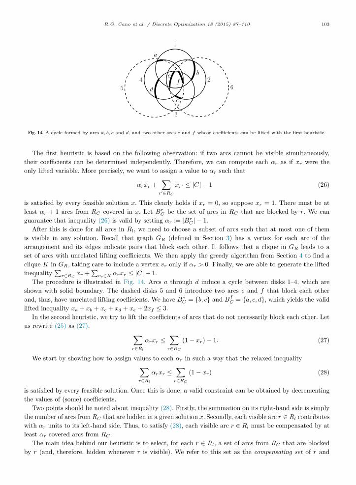
Fig. 14. A cycle formed by arcs a, b, c and d, and two other arcs e and f whose coefficients can be lifted with the first heuristic.
The first heuristic is based on the following observation: if two arcs cannot be visible simultaneously,their coefficients can be determined independently. Therefore, we can compute each αr as if xr were theonly lifted variable. More precisely, we want to assign a value to αr such that
αrxr +r′∈RC
xr′ ≤ |C| − 1 (26)
is satisfied by every feasible solution x. This clearly holds if xr = 0, so suppose xr = 1. There must be atleast αr + 1 arcs from RC covered in x. Let BrC be the set of arcs in RC that are blocked by r. We canguarantee that inequality (26) is valid by setting αr := |BrC | − 1.
After this is done for all arcs in Rl, we need to choose a subset of arcs such that at most one of themis visible in any solution. Recall that graph GR (defined in Section 3) has a vertex for each arc of thearrangement and its edges indicate pairs that block each other. It follows that a clique in GR leads to aset of arcs with unrelated lifting coefficients. We then apply the greedy algorithm from Section 4 to find aclique K in GR, taking care to include a vertex vr only if αr > 0. Finally, we are able to generate the liftedinequality
r∈RC xr +
vr∈K αrxr ≤ |C| − 1.
The procedure is illustrated in Fig. 14. Arcs a through d induce a cycle between disks 1–4, which areshown with solid boundary. The dashed disks 5 and 6 introduce two arcs e and f that block each otherand, thus, have unrelated lifting coefficients. We have BeC = {b, c} and BfC = {a, c, d}, which yields the validlifted inequality xa + xb + xc + xd + xe + 2xf ≤ 3.
In the second heuristic, we try to lift the coefficients of arcs that do not necessarily block each other. Letus rewrite (25) as (27).
r∈Rl
αrxr ≤r∈RC
(1− xr)− 1. (27)
We start by showing how to assign values to each αr in such a way that the relaxed inequalityr∈Rl
αrxr ≤r∈RC
(1− xr) (28)
is satisfied by every feasible solution. Once this is done, a valid constraint can be obtained by decrementingthe values of (some) coefficients.
Two points should be noted about inequality (28). Firstly, the summation on its right-hand side is simplythe number of arcs from RC that are hidden in a given solution x. Secondly, each visible arc r ∈ Rl contributeswith αr units to its left-hand side. Thus, to satisfy (28), each visible arc r ∈ Rl must be compensated by atleast αr covered arcs from RC .
The main idea behind our heuristic is to select, for each r ∈ Rl, a set of arcs from RC that are blockedby r (and, therefore, hidden whenever r is visible). We refer to this set as the compensating set of r and
denote it by MrC . The value of each coefficient αr is then set to |MrC |. If two lifting candidates can be visiblesimultaneously, their compensating sets must be disjoint; otherwise, they may share some common elements.Next, we show that if this condition is obeyed, our choice of coefficients guarantees that (28) holds for allfeasible solutions.
Initially, observe that if an arc r ∈ Rl is visible, at least the arcs inMrC must be covered. Hence, inequality(29) is always satisfied.
r∈Rlxr=1
MrC
≤ r∈RC
(1− xr) . (29)
We now analyze the left-hand side of (29). Since we assume that the preceding condition is obeyed, allsets in the union are disjoint. This allows us to write
r∈Rlxr=1
MrC
= r∈Rlxr=1
|MrC |.
But the last summation just adds the coefficients of visible arcs. Thus, it is equal tor∈Rl αrxr and the
result follows.So far we are able to satisfy only (28) but not (27). A straightforward solution would be to decrement all
positive coefficients by one. However, it is possible to do better than this. If we can make sure that equalitynever occurs in (29), inequality (27) will be automatically satisfied. One way to do this is to prohibit onearc from each BrC from being included in any compensating set. This way, each time arc r is visible, thereis at least one hidden arc that is not accounted for in the left-hand side of (29). More precisely, we want toselect a set of arcs HC ⊆ RC such that HC ∩BrC = ∅ for all r ∈ Rl. This is simply the statement of a hittingset problem.
We are now able to describe our algorithm. We first select the arcs r ∈ Rl such that |BrC | ≥ 2. There isno need to consider the others because our heuristic cannot assign a positive coefficient to any of them. Wethen construct the set BrC for each selected arc r. A hitting set HC is found using a greedy heuristic thatselects, at each stage, the element that is contained in the largest number of sets that have not yet been hit.We make HC minimal by excluding unnecessary elements.
Next, we start building the compensating sets. Given an arc s ∈ RC −HC , let Bsl denote the set of arcsfrom Rl that block s. We need to choose an arc from Bsl and insert s into its compensating set. We wishto create an inequality with a large violation, so our strategy is to select the arc r with largest xr. Recallthat we are allowed to insert s in more than one compensating set as long as the associated arcs cannotbe visible together in a feasible solution. So, instead of picking a single arc from Bsl , we select a set of arcssuch that any two of them block each other. Again, such a set of arcs corresponds to a clique in graph GRand we can compute it the same way we did in the first heuristic. Finally, we generate the lifted inequalityr∈RC xr +
r∈Rl |M
rC |xr ≤ |C| − 1.
The procedure is depicted in Fig. 15. Arcs a through d induce a cycle between disks 1–4, which are shownwith solid boundary. The dashed disks 5, 6 and 7 introduce three arcs e, f and g whose coefficients we wantto lift. We have BeC = {a, b, c}, BfC = {c, d} and BgC = {b, c}. Thus, a possible hitting set is HC = {c}. Forthe remaining arcs, we have Bal = {e}, Bbl = {e, g} and Bdl = {f}. We can now create the compensatingsets. Arcs a and d can only be inserted in MeC and MfC , respectively. Arc b can be inserted in either MeC orMgC , but not both because e and g do not block each other. For this example, we choose to insert it intoMgC . Finally, the compensating sets are MeC = {a},MfC = {d} and MgC = {b}, which results in the liftedinequality xa + xb + xc + xd + xe + xf + xg ≤ 3.
As we show in Section 7, these lifting heuristics contribute a great deal to improving the dual boundsgenerated by our formulations. Although no guarantees are given in general as for the dimension of the faces
Fig. 15. A cycle formed by arcs a, b, c and d, and three other arcs e, f and g whose coefficients can be lifted with the second heuristic.
induced by the lifted inequalities, it can be easily shown that those obtained for Figs. 14 and 15 are, indeed,facet-defining (the proof is omitted for the sake of brevity).
7. Computational experiments
We assess the effectiveness of our solution approach through a series of computational experiments with60 real-world instances. Firstly, we evaluate the performance of our strategy to select the initial set ofinequalities. Secondly, we measure the impact of lifting on both the dual bounds and the total runningtimes. Finally, we compare models AM and GOM for the three problem variants addressed in this paper.For the sake of brevity, the tables show the results for the most challenging instances. Our complete set ofinstances is available in our web page [12].
7.1. Implementation details
The procedures were implemented in C++ and compiled with GCC 4.4.3. We build the arrangementswith CGAL 4.0 using exact arithmetic. The ILPs are solved with CPLEX 12.4. We apply a branch-and-cutalgorithm and use the conventional search supplied by CPLEX. We limit the time spent by the solver to atmost five hours per component. The experiments were run on an Intel Xeon X3430, 2.40 GHz CPU with8 GB RAM.
All instances are decomposed in a preprocessing phase with the techniques from [4]. We solve allcomponents and then recombine them to create an optimal solution for the whole instance. For the Max-Total variants, solution values and gaps are calculated disregarding arcs that are visible in every feasibledrawing. Primal solutions for the Max-Total and the Max–Min problems are generated with the GRASPheuristic from [7] and with the greedy algorithm from [3], respectively.
As observed by Kunigami et al. [4], it is sometimes possible to bypass the resolution of integer programswhen solving the Max–Min PRDP. If an instance (or a component thereof) has a face that is containedin every disk, all physically realizable solutions must also be stacking drawings. This allows us to use thepolynomial time algorithm from Cabello et al. [3]. Besides that, not all components need to be solvedoptimally. We just need an optimal solution to the one that determines the Max–Min value. For the others,it often suffices to find a good heuristic solution, which can once again be done with the algorithm from [3].
7.2. Problem instances
We test our model on three sets of instances. The first set was presented by Cabello et al. [3] andcontains four instances: City 156 and City 538, which represent the 156 and 538 largest American cities,
Table 1Results for the initial linear relaxation using the model with all 2-cycle inequalities and the reduced one based on maximal arcs.Times are given in seconds.
Instance |S| |R| % Gaps Number of inequalities Relaxation timesAll Max. All Max. Ratio All Max. Ratio
respectively; and Deaths and Magnitudes, which represent the death count and the Richter scale magnitudeof 602 earthquakes worldwide, respectively.
The two other sets were used in [4,7] and contain 28 instances each. They were generated from data onthe population of cities from several countries. We refer to them as Population-S1 and Population-S2. Theyare both based on the same data, but with different proportionality constants between the area of the disksand the numerical values they represent. The instances in Population-S2 are scaled in such a way that thearea of each disk is twice as large as that in the analogous instance from Population-S1.
7.3. Numerical results
We first address the issue of selecting the initial set of inequalities that are loaded into the ILP solver.We compare the technique based on maximal arcs with the alternative of using all 2-cycle inequalities. Weremark that, as mentioned in Section 4, the latter is similar to starting with an empty model. It should alsobe noted that the techniques are the same for both stacking and physically realizable drawings. For thisreason, it is not necessary to show the results for each problem variant. In the text that follows, duality gapsare calculated with respect to Max-Total SDP optimal values.
Table 1 shows the results obtained after solving the linear relaxation of the initial set of inequalities. Foreach instance, we report the number of disks and arcs, the duality gap, the number of inequalities in thelinear program and the time spent solving the relaxation. Columns All and Max refer to the model with all2-cycle inequalities and to the reduced one based on maximal arcs, respectively. We also present the ratiosbetween the results of the two alternatives.
Using the reduced set of constraints increased the duality gaps by only 0.60% on average. The largestincrease occurred for instance Greece-S1 and, still, it was less than 4.00%. On average, the reduced modelhas 8.5 times fewer inequalities and the relaxation is solved 23.2 times faster. The most remarkable reductionoccurs for instance France-S2, which runs more than 1285 times faster with an increase of only 0.55% inthe duality gap. Due to the effectiveness of this strategy, all experiments that follow use this reduced set ofinequalities.
In the next experiment, we evaluate the impact of lifting on the dual bounds produced by our model.For each instance, we solve the root node of the branch-and-bound tree, which involves solving a linear
relaxation and then executing our separation routines. This procedure is repeated until no more violatedinequalities are found. Automatic cut generation routines were disabled during this experiment. The resultsare shown in Table 2. The original arc model is denoted by AM, whereas the improved formulation obtainedafter the inclusion of lifting is denoted by AM++. We report the duality gaps after solving the root node ofthe enumeration tree.
The results show that the behavior for both Max-Total problems is very similar. Although AM leaves asmall gap, it can still lead to a relatively costly branching. The addition of lifting makes all gaps drop toless than 0.26% and 18 instances that would otherwise need branching can be optimally solved at the rootnode. As for the Max–Min PRDP, due to the need of a continuous variable to model the objective function,duality gaps are significantly larger. Nevertheless, the lifting procedures are still able to reduce the gaps formany instances.
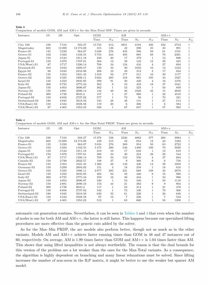
In the final experiment, we run models GOM, AM and AM++ on all instances for the three problemvariants. We enable automatic cut generation routines to evaluate the performance of the models inconjunction with the most advanced features provided by the solver. The results are shown in Tables 3–5.Optimal values are given in column Opt. For each model, we report the total running time (in seconds), thenumber of cuts NC added by our separation routines and the number of nodes NN solved in the branch-and-bound tree. Some preliminary tests indicated that the GOM model also benefits from the inclusion ofthe initial set of inequalities described in this work. To establish a fair comparison between the models, theresults that follow incorporate these improvements.
To further analyze the speedup enabled by each model, Table 6 shows, for each pair of models, theaverage, maximum and minimum ratio of their running times. To focus on the hardest instances, the resultsdisregard those that can be solved in less than 10 s by both models. Average values are computed as thegeometric mean of the running time ratios.
For both Max-Total variants, the results show that AM performs better than GOM for all instances. Thereduction in the number of variables compensates for the exponential number of inequalities and the arc-based formulation achieves a (geometric) average speedup of 5.9 and 6.0 for the SDP and PRDP variants,respectively. The addition of lifting allows AM++ to run 1.9 times faster than AM for both types ofdrawings. Besides, all but two instances are solved in the root node of the branch-and-bound tree. Thegreatest improvements occurred for instances France-S1 and Greece-S1, for which AM++ is over 82 timesfaster than GOM for SDP.
It is interesting to note that, as shown in Table 2, AM is never able to completely solve the problemon the root node of the search tree. However, in this experiment, this was possible due to the inclusion of
automatic cut generation routines. Nevertheless, it can be seen in Tables 3 and 4 that even when the numberof nodes is one for both AM and AM++, the latter is still faster. This happens because our specialized liftingprocedures are more effective than the generic cuts added by the solver.
As for the Max–Min PRDP, the arc models also perform better, though not as much as in the othervariants. Models AM and AM++ achieve faster running times than GOM in 48 and 47 instances out of60, respectively. On average, AM is 1.99 times faster than GOM and AM++ is 1.04 times faster than AM.This shows that using lifted inequalities is not always worthwhile. The reason is that the dual bounds forthis version of the problem are a lot weaker than the ones for the Max-Total variants. As a consequence,the algorithm is highly dependent on branching and many linear relaxations must be solved. Since liftingincreases the number of non-zeros in the ILP matrix, it might be better to use the weaker but sparser AMmodel.
A single instance (Switzerland-S2) could not be solved by any of the models within the imposed timelimit. The optimal value shown in Table 5 was verified after almost 54 h of computation with the AM model,which is the one that presented the best prospects after the initial five hours.
For the three problem variants, the number of cuts added by our separation routines range from a coupleof hundreds to a few thousands. A comparison with the initial number of inequalities reported in Table 1indicates that the size of the models is not significantly affected by the inclusion of these constraints. For mostinstances, AM++ adds considerably more cuts than AM. This behavior is expected because, as explainedin Section 5, our lifting heuristics are applied not only to violated inequalities (2) and (3), but also to thosethat are satisfied with a small slack.
8. Conclusion
We study three variants of a proportional symbol maps problem and propose a novel ILP model in termsof arc variables only. We show that our model for stacking drawings is a projection of another one previouslydescribed in the literature. In addition, we describe a strategy to select the initial set of inequalities thatgreatly improves computation times not only with our models but also with another one from the literature.We also describe fast separation routines and effective lifting procedures. When compared with state-of-the-art models, our formulations significantly reduce computation times for most instances. In particular, forthe Max-Total variants, 57 out of 60 instances can now be solved in less than a minute.
Several directions exist for future research. From a theoretical perspective, two interesting possibilities aredeciding on the computational complexity of the Max-Total SDP and determining whether the AM modelfor PRDP is also a projection of GOM for that variant. Other ideas include the study of new facet-defininginequalities and the development of branching techniques based on geometric properties of the problem.
Finally, current methods still require large computation times to solve the Max–Min PRDP exactly, so thereis still a lot of room for improvement.
References
[1] B. Dent, Cartography—Thematic Map Design, fifth ed., McGraw-Hill, 1999.[2] T.A. Slocum, R.B. McMaster, F.C. Kessler, H.H. Howard, Thematic Cartography and Geographic Visualization, second
ed., Prentice Hall, 2003.[3] S. Cabello, H. Haverkort, M. van Kreveld, B. Speckmann, Algorithmic aspects of proportional symbol maps, Algorithmica
58 (3) (2010) 543–565.[4] G. Kunigami, P.J. de Rezende, C.C. de Souza, T. Yunes, Generating optimal drawings of physically realizable symbol
maps with integer programming, Vis. Comput. 28 (10) (2012) 1015–1026.[5] G. Kunigami, P.J. de Rezende, C.C. de Souza, T. Yunes, Optimizing the layout of proportional symbol maps: Polyhedra
and computation, INFORMS J. Comput. 26 (2) (2014) 199–207.[6] G. Kunigami, Proportional symbol maps (Master’s thesis) Institute of Computing, University of Campinas, Brazil, 2011.[7] R.G. Cano, G. Kunigami, C.C. de Souza, P.J. de Rezende, A hybrid GRASP heuristic to construct effective drawings of
proportional symbol maps, Comput. Oper. Res. 40 (5) (2012) 1435–1447.[8] G. Nivasch, J. Pach, G. Tardos, The visible perimeter of an arrangement of disks, in: W. Didimo, M. Patrignani (Eds.),
Proceedings of the 20th International Symposium on Graph Drawing, in: Lecture Notes in Computer Science, vol. 7704,Springer-Verlag, 2013, pp. 364–375.
[9] M. Grotschel, M. Junger, G. Reinelt, On the acyclic subgraph polytope, Math. Program. 33 (1) (1985) 28–42.[10] R. Muller, On the partial order polytope of a digraph, Math. Program. 73 (1996) 31–49.[11] E. Balas, M. Oosten, On the dimension of projected polyhedra, Discrete Appl. Math. 87 (1–3) (1998) 1–9.[12] G. Kunigami, R.G. Cano, P.J. de Rezende, C.C. de Souza, Proportional Symbol Maps—Benchmark Instances, 2011.