Linear equalities in blackbox optimization ∗

Charles Audet† Sebastien Le Digabel‡ Mathilde Peyrega§

May 28, 2014

Abstract: The Mesh Adaptive Direct Search (MADS) algorithm is designed for black-box optimization problems subject to general inequality constraints. Currently, MADS

does not support equalities, neither in theory nor in practice. The present work proposesextensions to treat problems with linear equalities whose expression is known. The mainidea consists in reformulating the optimization problem into an equivalent problem with-out equalities and possibly fewer optimization variables. Several such reformulations areproposed, involving orthogonal projections, QR or SVD decompositions, as well as sim-plex decompositions into basic and nonbasic variables. All of these strategies are studiedwithin a unified convergence analysis, guaranteeing Clarke stationarity under mild condi-tions provided by a new result on the hypertangent cone. Numerical results on a subset ofthe CUTEst collection are reported.

Keywords Derivative-free optimization, blackbox optimization, linear equality constraints,convergence analysis, MADS.

1 IntroductionIn some optimization problems, the objective function, as well as the functions definingthe constraints, may be analytically unknown. They can instead be the result of an experi-ment or a computer simulation, and, as a consequence, they may be expensive to evaluate,be noisy, possess several local optima, and even return errors at a priori feasible points.Moreover, derivatives are unavailable and cannot be estimated, even when they exist, andtherefore cannot be used for optimization. Derivative-free optimization (DFO) methods,

∗Work of the first author was supported by NSERC grant 239436. The second author was supported byNSERC grant 418250. The first and second authors are supported by AFOSR FA9550-12-1-0198.†GERAD and Departement de mathematiques et genie industriel, Ecole Polytechnique de Montreal, C.P.

6079, Succ. Centre-ville, Montreal, Quebec, Canada H3C 3A7, www.gerad.ca/Charles.Audet.‡GERAD and Departement de mathematiques et genie industriel, Ecole Polytechnique de Montreal, C.P.

6079, Succ. Centre-ville, Montreal, Quebec, Canada H3C 3A7, www.gerad.ca/Sebastien.Le.Digabel.§GERAD and Ecole Polytechnique de Montreal, C.P. 6079, Succ. Centre-ville, Montreal, Quebec,

Canada H3C 3A7, www.github.com/mpeyrega, mathilde.peyrega@polymtl.ca.

1

and more precisely direct-search methods, are designed to handle these cases by consid-ering only the function values. From aeronautics to chemical engineering going throughmedical engineering and hydrology, these algorithms have several applications in a widerange of fields. More details about these methods and their applications in numerous fieldsare exposed in the book [11] and in the recent survey [3].

The present work proposes a direct-search algorithm for blackbox optimization prob-lems subject to general inequality constraints, lower and upper bounds, and linear equal-ities. Without any loss of generality, we consider only the linear equalities of the typeAx = 0, whereA is known a priori and is a full row rank matrix. A simple linear translationcan be applied to nullify a nonzero right-hand-side. We consider optimization problems ofthe following form:

minx∈Rnx

F (x) (1)

subject to C(x) ≤ 0

Ax = 0

L ≤ x ≤ U,

where A ∈ Rm×nx is full row rank matrix, L,U ∈ (R ∪ −∞ ∪ +∞)nx are boundvectors, possibly infinite, F : Rnx → R ∪ +∞ is a single-valued objective function, C:Rnx → (R ∪ +∞)p is the vector of constraints, and nx, m, p ∈ N are finite dimensions.Allowing the objective and inequality constraints to take infinite values is convenient ina minimization context for modeling situations in which the simulation failed to return avalid value.

An example of such a linear constrained derivative-free problems is exposed in [16].Even if there is only one linear equality treated with a simple variable substitution, it sug-gests that other examples with more linear equalities should emerged from chemical en-gineering. Moreover, solving this kind of problems can have applications even to designmore general DFO algorithms. Indeed, the authors of [6] design such algorithm for non-linear constrained blackbox optimization. At each iteration, their method needs to solvelinear equality constrained subproblems.

The objective of the present paper is to treat linear equalities with MADS by usingvarious reformulations of the problem, seen as a wrapper on the original problem. Inaddition, we prove a new result on the hypertangent cone, which allows to extend theMADS convergence theory.

The document is organized as follows. Section 2 reviews literature about equalities inDFO. Section 3 presents the basic framework to transform Problem (1) into a problem onwhich MADS can be applied, as well as a proof that, under mild conditions, this frame-work inherits the MADS convergence properties. Section 4 then introduces four classes oftransformations implementing the basic framework, and Section 5 illustrates the efficiencyof these transformations, as well as some hybrid strategies. We conclude with a discussionand future work in Section 6.

2

2 Handling linear constraints in DFO

Derivative-free algorithms may be partitioned into direct-search and model-based methods.At each iteration, direct-search methods evaluate the functions defining the problem (theblackbox) at a finite number of points and take decision for the next step based on thesevalues. In model-based methods, models are constructed to approximate the blackbox andare then optimized to generate candidates where to evaluate the blackbox.

The first direct-search algorithm considering linearly constrained problems is proposedby May [25]. It extends Mifflin’s derivative-free unconstrained minimization algorithm [26],an hybrid derivative-free method combining direct-search ideas with model-based tools.May’s main contribution is to use positive generators of specific cones which are approx-imation of the tangent cones of the active constraints. He proves both global convergenceand superlinear local convergence under assumptions including continuous differentiabil-ity of F . Later, Lewis and Torczon [21] proposed the Generalized Pattern Search (GPS)algorithm [33] to treat problems subject to linear inequalities. Under assumptions includ-ing continuous differentiability of F and rationality of the constraints matrix, they showconvergence to a KKT point, even in the presence of degeneracy. Other improvements todeal with degeneracy are proposed in [2], and similar ideas are given in [24] where theunconstrained GPS algorithm is adapted with directions in the nullspace of the matrix A.Coope and Price extended these ideas to a grid-base algorithm [12] by aligning the positivebasis with the active set of linear constraints [31]. These extensions were adapted to theGenerating Set Search (GSS) method [14, 19, 22, 20], which allows a broader selectionof search directions at the expense of imposing a minimal decrease condition in order toaccept a new incumbent solution. The positive basis for GSS at each iteration is chosen inthe nullspace of active equality constraints. This approach reduces the dimension of theproblem, because the search directions at each iteration are contained in a subspace. Refer-ences [18] and [23] present an algorithm for differentiable nonlinear problems with nonlin-ear equality and inequality constraints. An augmented Lagrangian method is adapted in theGSS framework, which provides a special treatment for linear constraints. This method fordifferentiable equalities and inequalities was first proposed in a trust-region context in [9].These ideas are implemented in the HOPSPACK software package [29].

Derivative-free trust-region methods are a class of model-based algorithms, using re-gression or interpolation. The theory considers no constraints but it can be easily adaptedto bound and linearly constrained problems [11]. Moreover, the equalities are used to re-duce the degrees of freedom of the problem [10]. In the LINCOA package [30], Powellproposes an implementation of a derivative-free trust-region algorithm considering linearinequality contraints by using an active set method.

The Mesh Adaptive Direct Search (MADS) algorithm [4] is a direct-search methodgeneralizing GPS and designed for bound-constrained blackbox problems. Its convergenceanalysis is based on the Clarke calculus [8] for nonsmooth functions. Inequalities includinglinear constraints are treated with the progressive barrier technique of [5], and equalityconstraints are not currently supported. The idea exposed in Section 3 is to treat linearequalities by designing a wrapper and a converter to transform the initial Problem (1) into

3

a problem on which MADS can be applied.

3 Reformulations without linear equalitiesThe approach of this work consists to reformulate Problem (1) in order to eliminate thelinear constraints Ax = 0 and then, apply the MADS algorithm to the reformulation. Thefollowing notation is used throughout the paper. Let S = x ∈ Rnx : Ax = 0 denote thenullspace of the matrix A, and Ωx = x ∈ S : C(x) ≤ 0, L ≤ x ≤ U the set of feasiblesolutions to Problem (1).

A straightforward suggestion is to transform the linear equality Ax = 0 into two in-equalities, and to include them to the inequality constraints C(x) ≤ 0, as suggested in theLINCOA package [30]. However, this method is unsuitable in our context for both theo-retical and practical issues. First, existing convergence analysis of MADS would be limitedto its most basic result. The convergence analysis of MADS leading to Clarke stationarityrequires that the hypertangent cone to the feasible set Ωx is non-empty at some limit point(Section 3.3 of the present document presents the definition of the hypertangent cone rel-ative to a subspace). However, in the presence of linear equalities, the hypertangent coneis necessarily empty for every x ∈ Rnx . This is true because the cone is either emptyor its dimension is equal to N [8]. Second, almost all evaluations will occur outside ofthe linear subspace S. The extreme barrier [4] will reject these points, or the progressivebarrier [5] will invest most of its effort in reaching feasibility rather than improving theobjective function value. This explains that splitting an equality into two inequalities failsin practice, as observed in [6].

The ideas introduced for GPS and GSS as described in the previous section could alsobe implemented in MADS. Instead of choosing orthogonal positive bases in the entirespace Rnx to generate the mesh in MADS, it is possible to choose a positive basis of S, andto complete it by directions in Rnx \ S in order to obtain a positive basis of Rnx . Thesedirections would be pruned by the algorithm because they generate points outside of S.Some of the strategies presented in Section 4 can be seen as particular instantiations of thisapproach. However, we prefer to view them from a different perspective.

3.1 Inequality constrained reformulationIn order to reformulate Problem (1) into an inequality constrained optimization problemover a different set of variables in Rnz , we introduce the following definition.

Definition 3.1 A converter ϕ is a surjective linear application from Rnz to S ⊂ Rnx , forsome nz ∈ N. For any x ∈ S, there exists an element z ∈ Rnz such that x = ϕ(z).

By definition, a converter ϕ is continuous, and any z ∈ Rnz is mapped to an x =ϕ(z) ∈ Rnx that satisfies the linear equalities Ax = 0. Since dim S is equal to nx −m, itfollows that nz ≥ nx −m. Furthermore, nz equals nx −m if and only if the converter isbijective.

4

A converter ϕ is used to perform a change of variables, and to reformulate Problem (1)as follows:

minz∈Rnz

f(z)

subject to c(z) ≤ 0L ≤ ϕ(z) ≤ U .

(2)

where f : Rnz → (R ∪ +∞) and c : Rnz → (R ∪ ±∞)p are defined by:

f(z) = F (ϕ(z)) and c(z) = C(ϕ(z)) .

Let Ωz = z ∈ Rnz : c(z) ≤ 0 and L ≤ ϕ(z) ≤ U denote the set of feasible solutions forthe reformulated Problem (2). The following proposition details the connection betweenthe sets of feasible solutions for both sets of variables x and z.

Proposition 3.2 The image of Ωz by the converter ϕ is equal to Ωx, and the inverse imageof Ωx by converter ϕ is equal to Ωz:

Ωx = ϕ(Ωz) and Ωz = ϕ−1(Ωx) := z ∈ Rnz : ϕ(z) ∈ Ωx.

PROOF. By construction we have ϕ(Ωz) ⊂ Ωx = x ∈ S : C(x) ≤ 0, L ≤ x ≤ U.In addition, as ϕ is subjective, for any x ∈ Ωx ⊂ S, there exists some z ∈ Rnz suchthat ϕ(z) = x. Since x belongs to Ωx, it follows that C(ϕ(z)) ≤ 0 and L ≤ ϕ(z) ≤ U .Therefore, z ∈ Ωz and x ∈ ϕ(Ωz). This implies that Ωx ⊂ ϕ(Ωz).

Conversely, as Ωx is equal to ϕ(Ωz) and by the definition of the inverse image, we haveΩz ⊂ ϕ−1(Ωx). Moreover, if z ∈ ϕ−1(Ωx), then ϕ(z) ∈ Ωx and z ∈ Ωz. This implies thatϕ−1(Ωx) ⊂ Ωz.

3.2 Applying MADS on a reformulationThe converter is used to construct a wrapper around the original optimization problemso that the MADS algorithm is applied to the reformulated one. Figure 1 illustrates theapplication of the MADS algorithm to Problem (2). MADS proposes trial points z ∈ Rnz ,which are converted into x = ϕ(z) belonging to the nullspace S. If x is within the boundsof the original optimization problem, then the blackbox simulation is launched to evaluateF (x) and C(x). Otherwise, the cost of the simulation is avoided and F (x) and C(x) arearbitrarily set to an infinite value. In both cases, the outputs are assigned to f(z) and c(z),and returned to the MADS algorithm.

The MADS algorithm can be applied to Problem (2) and the constraints can be par-titioned into two groups. The constraint functions c(z) are evaluated by launching theblackbox simulation; the constraints L ≤ ϕ(z) ≤ U are checked a priori, before executingthe blackbox. When these constraints are not satisfied for a given z ∈ Rnz , the cost oflaunching the blackbox is avoided.

5

Wrapper

MADS

ϕ @

@@@

@@@@

L ≤ x ≤ U

Blackbox

F (x) =∞C(x) =∞

-

z ∈ Rnz

z -x = ϕ(z)

-x

YES?

F (x)

C(x)

-NO6

F (x)

C(x)

-

?f(z) = F (x)

c(z) = C(x)

Figure 1: The converter ϕ allows the construction of a wrapper around the original black-box.

A preprocessing phase can be executed to delimit more precisely the domain Ωz. Foreach i ∈ 1, 2, . . . , nz, solving the following linear programs yields valid lower and upperbounds `, u ∈ Rnz on z:

`i = min zi : L ≤ ϕ(z) ≤ U, z ∈ Rnz ,ui = max zi : L ≤ ϕ(z) ≤ U, z ∈ Rnz .

Thus, the problem that MADS considers in practice, equivalent to Problems (1) and (2),is the following:

minz∈Rnz

f(z)

subject to c(z) ≤ 0L ≤ ϕ(z) ≤ U` ≤ z ≤ u .

(3)

The feasible set for this problem is Ωz, as for Problem (2). The difference is that the bounds` and u may be used by MADS to scale the variables.

3.3 Convergence AnalysisThe fundamental convergence result [4] of MADS studies some specific accumulationpoints of the sequence of trial points in Rnz . In the proposed approach, the original prob-lem is formulated in Rnx , but the algorithm is deployed in Rnz . Our convergence analysis

6

consists in transposing the theoretical results from Rnz to the nullspace S ⊂ Rnx , whichcontains the entire sequence of trial points.

We use superscripts to distinguish vector spaces. For example, if E is a normed vectorspace like Rnz ,Rnx , or S, we will denote the open ball of radius ε > 0 centred at x ∈ Eby:

BEε (x) := y ∈ E : ||y − x|| < ε .

The convergence analysis relies on the following definition of the Clarke derivativetaken from [17] and adapted with our notations.

Definition 3.3 Let Ω be a nonempty subset of a normed vector space E, g : Ω −→ R beLipschitz near a given x ∈ Ω, and let v ∈ E. The Clarke generalized derivative at x in thedirection v is:

g(x; v) := lim supy → x, y ∈ Ω

t ↓ 0, y + tv ∈ Ω

g(y + tv)− g(y)

t. (4)

An important difference with previous analyses of MADS is that E may be a strictsubset of a greater space. For example, in our context, E corresponds to the nullspace S,strictly contained in Rnx , and Rnx is the native space of the original optimization problem.

The next definition describes the hypertangent cone THΩ (x) to a subset Ω ⊆ E at x,

where E is a normed vector space, as given by Clarke [8].

Definition 3.4 Let Ω be a nonempty subset of a normed vector space E. A vector v ∈ Eis said to be hypertangent to the set Ω at the point x ∈ Ω if there exists a scalar ε > 0 suchthat:

y + tw ∈ Ω for all y ∈ BEε (x) ∩ Ω, w ∈ BE

ε (v) and 0 < t < ε . (5)

The set of hypertangent vectors to Ω at x is called the hypertangent cone to Ω at x and isdenoted by TH

Ω (x).

A property of the hypertangent cone is that it is an open cone in the vector space E.The convergence analysis below relies on the assumption made for the MADS convergenceanalysis (see [4] for more details). The following theorem asserts that hypertangent conemapped by the converter ϕ coincides with the hypertangent cone in the nullspace S at thepoint mapped by ϕ.

Theorem 3.5 For every z ∈ Ωz, the hypertangent cone to Ωx at x = ϕ(z) in Rnz is equalto the image by ϕ of the hypertangent cone to Ωz at z in S. In other words,

THΩx

(ϕ(z)) = ϕ(THΩz

(z)) .

7

PROOF. The equality is shown by double inclusion. Both inclusions use the linearity ofthe converter ϕ and Proposition 3.2. The first inclusion is based on the continuity of ϕwhile the second requires the open mapping theorem [32]. The cases TH

Ωx(ϕ(z)) = ∅ and

THΩz

(z) = ∅ are trivial. In the following, let z be an element of the nonempty set Ωz.

First inclusion proof. Let v ∈ THΩx

(ϕ(z)) ⊆ S be an hypertangent vector to Ωx, andlet d ∈ Rnz be such that ϕ(d) = v. We show that d is hypertangent to Ωz at z. ByDefinition 3.4, choose ε > 0 such that:

y + tw ∈ Ωx for all y ∈ BSε (ϕ(z)) ∩ Ωx, w ∈ BS

ε (ϕ(d)) and 0 < t < ε . (6)

Continuity of ϕ and Proposition 3.2 allow to select ε1 > 0 and ε2 > 0 sufficiently small sothat:

ϕ(BRnz

ε1(z) ∩ Ωz) ⊂

(BS

ε (ϕ(z)) ∩ Ωx

)and ϕ(BRnz

ε2(d)) ⊂ BS

ε (ϕ(d)).

Let define εmin := minε1, ε2, ε, r ∈(BRnz

εmin(z) ∩ Ωz

), s ∈ BRnz

εmin(d), and 0 < t <

εmin. It follows that y := ϕ(r) ∈(BS

ε (ϕ(z)) ∩ Ωx

)and w := ϕ(s) ∈ BS

ε (ϕ(d)). Thus,Assertion (6) and linearity of ϕ ensure that:

ϕ(r + ts) = ϕ(r) + tϕ(s) = y + tw ∈ Ωx .

Finally, since Ωz = ϕ−1(Ωx), it follows that r + ts ∈ Ωz. Definition 3.4 is satisfied withr, s, t and εmin and therefore d ∈ TH

Ωz(z) implies that v = ϕ(d) ∈ ϕ(TH

Ωz(z)).

Second inclusion proof. Let d ∈ THΩz

(z) be an hypertangent vector to Ωz at z. We showthat ϕ(d) ∈ ϕ(TH

Ωz(z)) is hypertangent to Ωx at ϕ(z). By Definition 3.4, choose ε > 0 such

that:

r + ts ∈ Ωz for all r ∈ BRnz

ε (z) ∩ Ωz, s ∈ BRnz

ε (d) and 0 < t < ε.

The open mapping theorem [32] ensures that there exist ε1 > 0 and ε2 > 0 such that:

BSε1

(ϕ(z)) ⊂ ϕ(BRnz

ε (z)) and BSε2

(ϕ(d)) ⊂ ϕ(BRnz

ε (d)).

Define εmin := minε1, ε2, ε, and let

y ∈(BS

εmin(ϕ(z)) ∩ Ωx

), w ∈ BS

εmin(ϕ(d)) and 0 < t < εmin .

By the choice of εmin, it follows that y belongs to both sets ϕ(BRnz

ε (z)) and Ωx. Con-sequently, there exists an r ∈ BRnz

ε (z) such that y = ϕ(r), which also belongs to Ωz =ϕ−1(Ωx) since ϕ(r) ∈ Ωx. Let s ∈ BRnz

ε (d) be such thatw = ϕ(s). Applying the converterϕ yields:

y + tw = ϕ(r) + tϕ(s) = ϕ(r + ts) ∈ Ωx

since r + ts ∈ Ωz. Definition 3.4 is satisfied with y, w, t and εmin, and therefore ϕ(d) ∈TH

Ωx(ϕ(z)).

8

In our algorithmic framework, we apply the MADS algorithm to Problem (3) which isan equivalent reformulation of Problem (1). We use the standard assumptions [1, 4] thatthe sequence of iterates produced by the algorithm belongs to a bounded set, and that theset of normalized polling directions is asymptotically dense in the unit sphere. The MADS

convergence analysis [4] gives conditions ensuring the existence of a refined point, i.e., acluster point of the sequence of trial points at which f (z∗; v) ≥ 0 for every hypertangentdirection v ∈ TH

Ωz(z∗), provided that f is locally Lipschitz in z∗. However, this result holds

on the reformulated problem, and is not stated using the notations of the original equalityconstrained problem. The following theorem fills the gap by stating the main convergenceresult for Problem (3).

Theorem 3.6 Let x∗ be the image of a refined point z∗ produced by the application ofMADS on Problem (3): x∗ = ϕ(z∗). If F is locally Lipschitz near x∗, then:

F (x∗; v) ≥ 0 for all v ∈ THΩx

(x∗) .

PROOF. Let z∗ be a refined point produced by the application of MADS to Problem (3)and set x∗ := ϕ(z∗) be the corresponding point in the original space of variables.

Let v ∈ THΩx

(x∗) = THΩx

(ϕ(z∗)) be an hypertangent direction at x∗. By Proposition 3.5,let d ∈ TH

Ωz(z∗) be such that ϕ(d) = v.

If F is locally Lipschitz near x∗, and since ϕ is a linear application, then the definitionof f(z) = F (ϕ(z)) ensures that f is locally Lipschitz near z∗. The MADS convergenceresult holds: f (z∗; d) ≥ 0. By Definition (4), let rk → z∗ and sk → d be two sequencesin Ωz and let tk → 0 be a sequence in R such that:

f(rk + tksk)− f(rk) ≥ 0 for every k ∈ N.

The converted sequence yk := ϕ(rk) and wk := ϕ(sk) converge respectively tox∗ and v, and satisfy for every k ∈ N:

f(rk + tksk)− f(rk) ≥ 0 ⇐⇒ F (ϕ(rk + tksk))− F (ϕ(rk)) ≥ 0

⇐⇒ F (yk + tkwk)− F (yk) ≥ 0 .

which shows that F (x∗; v) ≥ 0.

Corollaries of this theorem can be developed as in [4] by analyzing smoother objectivefunctions, or by imposing more conditions on the domain Ωz. For example, by imposingstrict differentiability of F near x∗ and by imposing that Ωx is regular and that the hyper-tangent cone is nonempty, then one can show that x∗ is a contingent KKT stationary pointof F over Ωx.

9

4 Different classes of transformationsA converter is a surjective linear application. In this section, we present four different con-verters based on an orthogonal projection, SVD and QR decompositions, and a simplex-type decomposition that partitions the variables into basic and non-basis variables, as ex-posed in [28]. For each converter, we describe the ϕ function and show that it maps anyvector onto the nullspace S.

4.1 Orthogonal projectionDefine ϕP : Rnx → S as the orthogonal projection of the matrix A into the nullspace S.For each z ∈ Rnx , define:

ϕP (z) := (I − A+A)z ∈ S ⊂ Rnx

where A+ = AT (AAT )−1 is the pseudoinverse of A. The inverse of AAT exists because Ais of full row rank. If x = ϕP (z), then:

Ax = A(I − A+A)z = (A− AAT (AAT )−1A)z = 0

which confirms that x ∈ S. For this converter, nz = nx.

4.2 QR decompositionThe QR decomposition of the matrix AT ∈ Rnx×m is AT = QR, where Q ∈ Rnx×nx is anorthogonal matrix and R ∈ Rnx×m is an upper triangular matrix. Furthermore,

AT =(Q1 Q2

)(R1

0

)where Q1 ∈ Rnx×m and Q2 ∈ Rnx×(nx−m) are composed of orthonormal vectors, andR1 ∈ Rm×m is an upper triangular square matrix. Finally, 0 corresponds to the null matrixin R(nx−m)×m. For all z ∈ Rnx−m, the converter ϕQR : Rnx−m → S is defined as:

ϕQR(z) := Q2z .

If x = ϕQR(z), and since Q is an orthogonal matrix, then

Ax =(RT

1 0T)(QT

1

QT2

)Q2z =

(RT

1 0T)(0

I

)z = 0

which shows that x ∈ S. For this converter, nz = nx −m.

10

4.3 SVD decompositionUnlike the diagonalization which cannot be applied to every matrix, Singular Value De-composition (SVD) is always possible. The full row rank matrix A of Problem (1) can bedecomposed in A = UΣV T where U ∈ Rm×m and V ∈ Rnx×nx are unitary matrices, andΣ can be written as:

Σ =

σ1 · · · 0 0 · · · 0... . . . ... 0 · · · 00 · · · σm 0 · · · 0

∈ Rm×nx

for some positive scalars σi, i ∈ 1, 2, . . . ,m. Since U and V are unitary matrices, thenU−1 = UT and V −1 = V T . For all z ∈ Rnx−m, the converter ϕSV D : Rnx−m → S is definedas:

ϕSV D(z) := V

(0m

z

)where 0m is the null vector in Rm. If x = ϕSV D(z), then:

Ax = UΣV TV

(0m

z

)= UΣ

(0m

z

)= 0

and therefore x ∈ S. For this converter, nz = nx −m.

4.4 BN decompositionThis fourth converter uses the simplex-type decomposition into basic and nonbasic vari-ables. It reduces Problem (1) to one with dimension nx −m. The full row rank matrix Ahas more columns than rows. Let IB and IN form a partition of the columns of A such thatB = (Ai)i∈IB is a nonsingular m×m matrix, and N = (Ai)i∈IN is a m× (nx−m) matrix.The vector x is partitioned in the same way:

A = [B N ] and x =

(xBxN

)where xB = xi : i ∈ IB is of dimension m and xN = xi : i ∈ IN of dimensionnx − m. For any nonbasic variable xN ∈ Rnx−m, setting xB = −B−1NxN implies thatx satisfies the linear equalities. For all z ∈ Rnx−m, the converter ϕBN : Rnx−m → S isdefined as:

ϕBN(z) :=

(−B−1Nz

z

),

and if x = ϕBN(z), then

Ax = [B N ]

(−B−1Nz

z

)= −BB−1Nz +Nz = 0

11

which confirms that x ∈ S. The optimization problem on which MADS is applied hasnz = nx −m variables and can be written as follows:

minz∈Rnz

fBN(z)

subject to cBN(z) ≤ 0L ≤ ϕBN(z) ≤ U

(7)

where fBN(z) = F (ϕBN(z)) and cBN(z) = C(ϕBN(z)). Note that the choice of matrices(B,N) is not unique.

4.5 Comments on the convertersThe converters presented above reduce the dimension of the space of variables on whichMADS is applied from nx to nz = nx − m, where m is the number of linear equalities,except for the orthogonal projection technique of Section 4.1 for which the dimension re-mains nx. The projection is also the only transformation that is not bijective. For the firstthree converters (P, QR and SVD), the bounds L ≤ x ≤ U are translated into linearinequalities, which are treated as a priori constraints, as shown in Figure 1. The BN de-composition partitions the variables as basic and nonbasic variables, and optimizes over thenonbasic ones. Therefore, their bounds are simply Li ≤ zi ≤ Ui, for i ∈ 1, 2, . . . , nz.Moreover, these three first converters are uniquely determined. However, there are expo-nentially many ways to partition the variables into basic and nonbasic ones. A practicalway to identify a partition is described in Section 5.2 of the numerical experiments.

5 Implementation and numerical resultsThis section presents the implementation and numerical experiments of the strategies forhandling the linear equalities. First, the set of test problems is presented. Then, the fourconverters are compared. Finally, strategies combining different converters are proposed.All initial points considered in this section are publicly available at http://www.gerad.ca/Charles.Audet/publications.

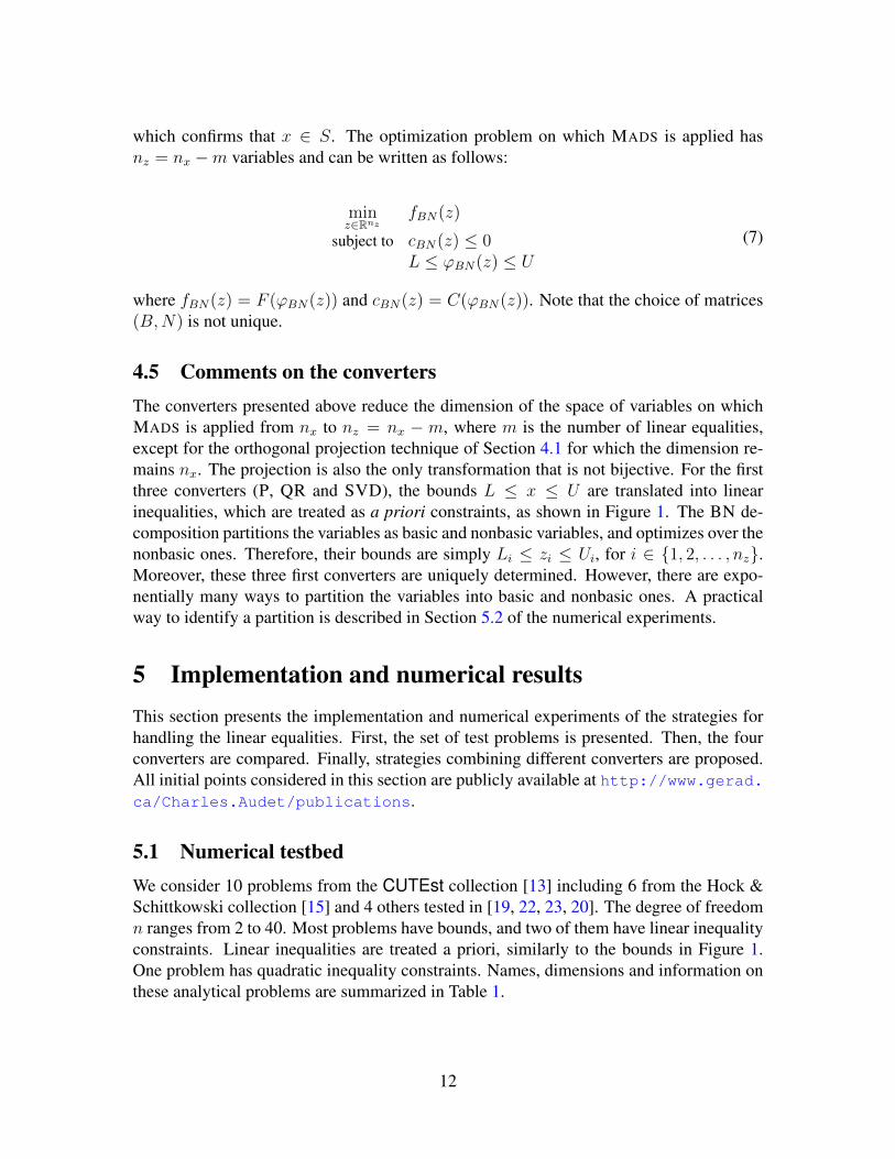
5.1 Numerical testbedWe consider 10 problems from the CUTEst collection [13] including 6 from the Hock &Schittkowski collection [15] and 4 others tested in [19, 22, 23, 20]. The degree of freedomn ranges from 2 to 40. Most problems have bounds, and two of them have linear inequalityconstraints. Linear inequalities are treated a priori, similarly to the bounds in Figure 1.One problem has quadratic inequality constraints. Names, dimensions and information onthese analytical problems are summarized in Table 1.

12

Name nx m n lower upper linear quad.bounds bounds ineq. ineq.

HS48 5 2 3 0 0 0 0HS49 5 2 3 0 0 0 0HS51 5 3 2 0 0 0 0HS53 5 3 2 5 5 0 0HS112 10 3 7 10 0 0 0HS119 16 8 8 16 16 0 0DALLASS 46 301 16 46 46 0 0LOADBAL 31 11 20 20 11 20 0AVION2 49 15 34 49 49 0 0PRODPl0 60 20 40 60 0 5 42

Table 1: Description of the 10 CUTEst analytical problems.

For each problem, 100 different initial feasible points are randomly generated, yieldinga total of 1,000 instances. Each instance is treated with a maximal budget of 100(n+1)objective function evaluations where n = nx −m is the degree of freedom.

In the next subsections, data profiles [27] are plotted to analyse the results. Thesegraphs compare a set of algorithms on a set of instances for a relative tolerance α ∈ [0; 1].Each algorithm corresponds to a plot where each couple (x, y) indicates the proportiony of problems solved within the relative tolerance α after x groups of n + 1 evaluations.The relative tolerance α is used to calculate the threshold below which an algorithm isconsidered to solve a specific instance successfully. This threshold is defined as the bestvalue obtained for this instance by any algorithm tested, with an added allowance of αmultiplied by the improvement between the initial value and that best value. The value ofα used in this section is set to 1%.

The NOMAD (version 3.6.0) and HOPSPACK (version 2.0.2) software packages areused with their default settings, except for the following: the use of models in NOMAD isdisabled, and the tolerance for the stopping criteria in HOPSPACK is set to 1E-13, whichis comparable to the equivalent NOMAD parameter. In HOPSPACK, the GSS algorithmnamed citizen 1 is considered.

5.2 BN analysis and implementation

There can be up to(nxm

)different partitions (IB, IN) of matrix A, and every choice is not

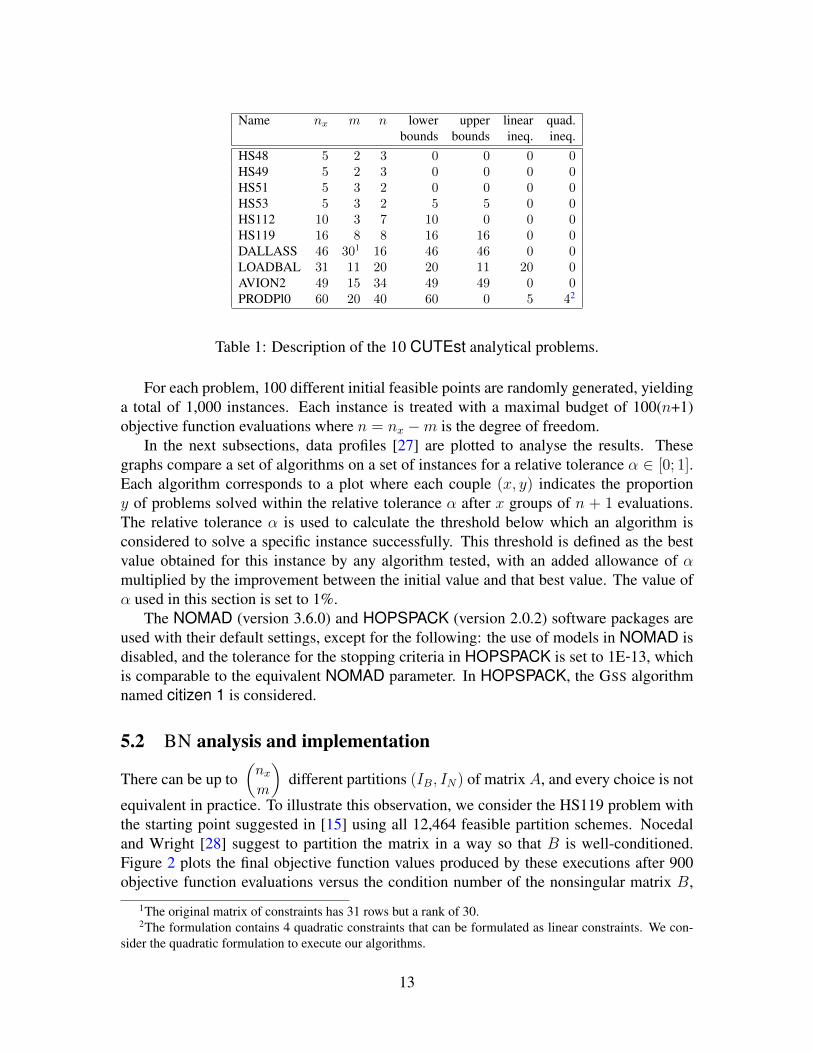
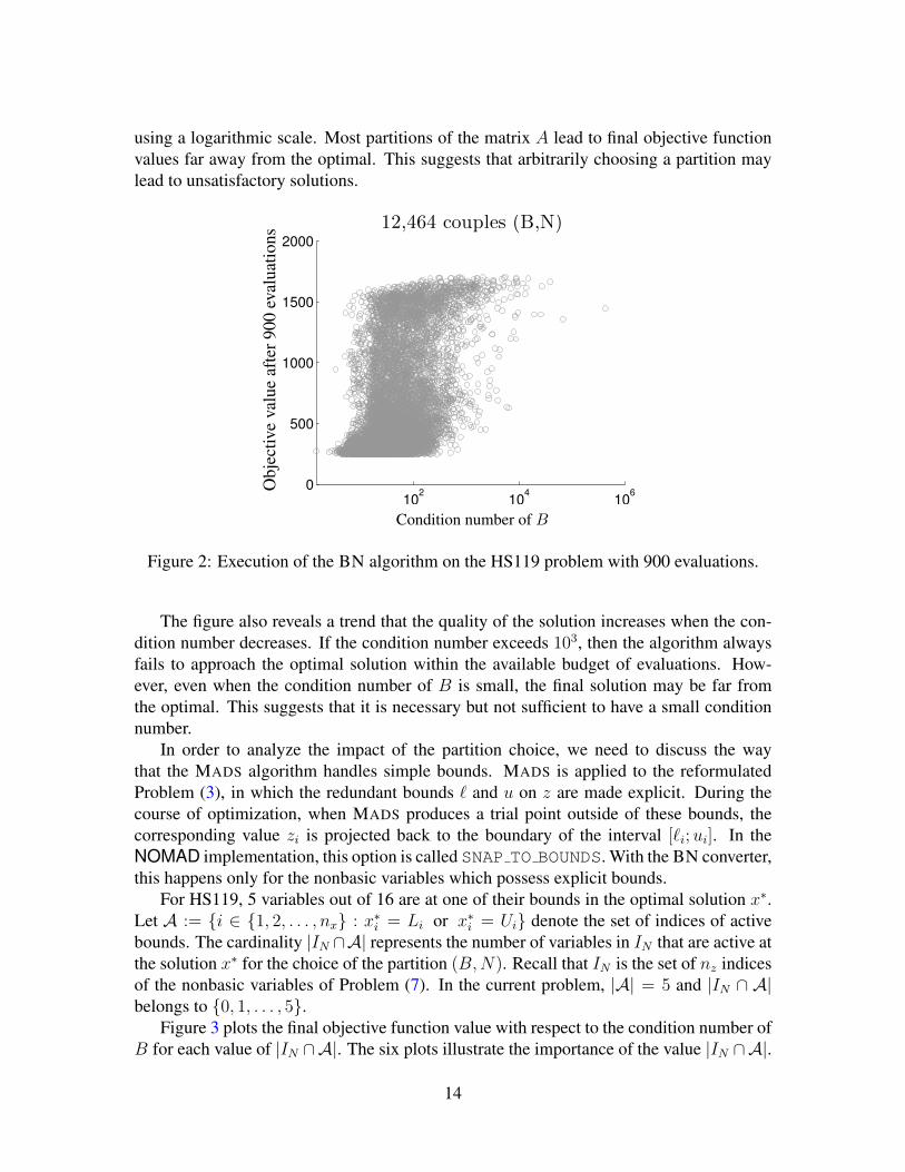
equivalent in practice. To illustrate this observation, we consider the HS119 problem withthe starting point suggested in [15] using all 12,464 feasible partition schemes. Nocedaland Wright [28] suggest to partition the matrix in a way so that B is well-conditioned.Figure 2 plots the final objective function values produced by these executions after 900objective function evaluations versus the condition number of the nonsingular matrix B,

1The original matrix of constraints has 31 rows but a rank of 30.2The formulation contains 4 quadratic constraints that can be formulated as linear constraints. We con-

sider the quadratic formulation to execute our algorithms.

13

using a logarithmic scale. Most partitions of the matrix A lead to final objective functionvalues far away from the optimal. This suggests that arbitrarily choosing a partition maylead to unsatisfactory solutions.

102

104

106

0

500

1000

1500

2000

12,464 couples (B,N)

Obj

ectiv

eva

lue

afte

r900

eval

uatio

ns

Condition number of B

Figure 2: Execution of the BN algorithm on the HS119 problem with 900 evaluations.

The figure also reveals a trend that the quality of the solution increases when the con-dition number decreases. If the condition number exceeds 103, then the algorithm alwaysfails to approach the optimal solution within the available budget of evaluations. How-ever, even when the condition number of B is small, the final solution may be far fromthe optimal. This suggests that it is necessary but not sufficient to have a small conditionnumber.

In order to analyze the impact of the partition choice, we need to discuss the waythat the MADS algorithm handles simple bounds. MADS is applied to the reformulatedProblem (3), in which the redundant bounds ` and u on z are made explicit. During thecourse of optimization, when MADS produces a trial point outside of these bounds, thecorresponding value zi is projected back to the boundary of the interval [`i;ui]. In theNOMAD implementation, this option is called SNAP TO BOUNDS. With the BN converter,this happens only for the nonbasic variables which possess explicit bounds.

For HS119, 5 variables out of 16 are at one of their bounds in the optimal solution x∗.Let A := i ∈ 1, 2, . . . , nx : x∗i = Li or x∗i = Ui denote the set of indices of activebounds. The cardinality |IN ∩A| represents the number of variables in IN that are active atthe solution x∗ for the choice of the partition (B,N). Recall that IN is the set of nz indicesof the nonbasic variables of Problem (7). In the current problem, |A| = 5 and |IN ∩ A|belongs to 0, 1, . . . , 5.

Figure 3 plots the final objective function value with respect to the condition number ofB for each value of |IN ∩A|. The six plots illustrate the importance of the value |IN ∩A|.

14

102

104

106

0

500

1000

1500

2000

|IN ∩ A| = 1

102

104

106

0

500

1000

1500

2000

|IN ∩ A| = 0

102

104

106

0

500

1000

1500

2000

|IN ∩ A| = 3

102

104

106

0

500

1000

1500

2000

|IN ∩ A| = 2

102

104

106

0

500

1000

1500

2000

|IN ∩ A| = 5

102

104

106

0

500

1000

1500

2000

|IN ∩ A| = 4O

bjec

tive

valu

eaf

ter9

00ev

alua

tions

Condition number of B

Figure 3: Final objective value for HS119 after 900 evaluations versus the condition num-ber. Each point represents a partition (IB, IN). Different graphics correspond to differentvalues of |IN ∩ A| ∈ 0, 1, . . . , 5.

When |IN ∩ A| = 5, all variables with an active bound are handled directly by MADS,and all runs converge to the optimal solution when the condition number is acceptable. As|IN ∩ A| decreases, the number of failed runs increases rapidly, even when the condition

15

number is low.Indices of active bounds at the solution as well as the condition number should influ-

ence the choice of the partition (IB, IN). However, optimizing the condition number is aNP-hard problem [7], and when solving an optimization problem from a starting point x0,one does not know which bounds will be active at the optimal solution. More elaboratesolutions overcoming these difficulties are proposed in Section 5.4 but a first method isproposed below.

The indices of the variables are sorted in increasing order with respect to the distance ofthe starting point to the bounds. Thus, the last indices of the ordered set will preferentiallybe chosen to form IB. More precisely, the index i appears before j if the distance fromx0i to its closest bound is more than or equal to the distance from x0

j to its closest bound.When both bounds are finite, the distances are normalized by the distance between thesebounds. Variables with only one finite bound come after the variable with two bounds inthe sorted set. Ties are broken arbitrarily.

The columns of A are sorted in the same order than the indices of the variables andthe following heuristic is applied to take into account the condition number. Construct anonsingular matrix B′ of m independent columns of A by adding the last columns of theorder set. Then let c be the next column of the ordered set that does not belong to B′.Define B to be the m ×m nonsingular matrix composed of columns of B′ ∪ c that hasthe smallest condition number. This requires to compute m condition numbers.

5.3 Comparison of the four converters with HOPSPACK

A first set of numerical experiments compares the four converters BN, QR, SVD and Pto the HOPSPACK software package on the 1,000 instances. In the case of the algorithmBN, the partition into the matrices B and H is done by considering the initial points andbounds, as explained in Section 5.2. A more extensive analysis of BN is presented inSection 5.4.

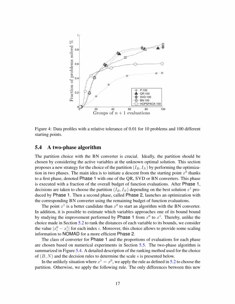
Comparison of the different converters with HOPSPACK is illustrated in Figure 4. Theconverter ϕP associated to the projection is dominated by all other strategies. This is notsurprising since the projection does not reduce the size of the space of variables in whichthe optimization in performed.

When the number of function evaluations is low, it seems that HOPSPACK performsbetter than the other methods. However, inspection of the logs reveals that this dominationis exclusive to the smallest problems, for which HOPSPACK does very well. For thelarger ones, QR, SVD and BN perform better than HOPSPACK.

The figure also reveals that BN, QR and SVD classes of converters outperforms theprojection, but it is not obvious to differentiate them. The next section proposes a way tocombine these converters.

16

0 20 40 60 80 1000

0.2

0.4

0.6

0.8

1

Groups of n+ 1 evaluations

Fractionofproblemssolved

%

P:100

QR:100

SVD:100

BN:100

HOPSPACK:100

Figure 4: Data profiles with a relative tolerance of 0.01 for 10 problems and 100 differentstarting points.

5.4 A two-phase algorithmThe partition choice with the BN converter is crucial. Ideally, the partition should bechosen by considering the active variables at the unknown optimal solution. This sectionproposes a new strategy for the choice of the partition (IB, IN) by performing the optimiza-tion in two phases. The main idea is to initiate a descent from the starting point x0 thanksto a first phase, denoted Phase 1 with one of the QR, SVD or BN converters. This phaseis executed with a fraction of the overall budget of function evaluations. After Phase 1,decisions are taken to choose the partition (IB, IN) depending on the best solution x1 pro-duced by Phase 1. Then a second phase, called Phase 2, launches an optimization withthe corresponding BN converter using the remaining budget of function evaluations.

The point x1 is a better candidate than x0 to start an algorithm with the BN converter.In addition, it is possible to estimate which variables approaches one of its bound boundby studying the improvement performed by Phase 1 from x0 to x1. Thereby, unlike thechoice made in Section 5.2 to rank the distances of each variable to its bounds, we considerthe value |x0

i − x1i | for each index i. Moreover, this choice allows to provide some scaling

information to NOMAD for a more efficient Phase 2.The class of converter for Phase 1 and the proportions of evaluations for each phase

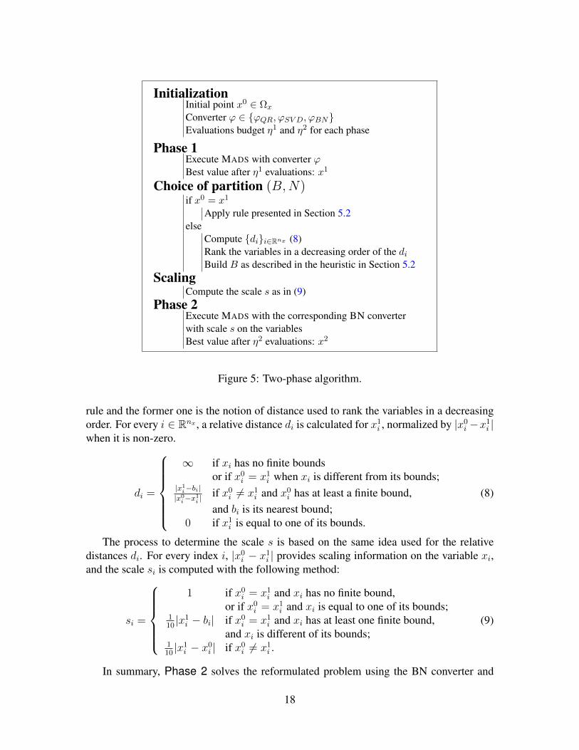
are chosen based on numerical experiments in Section 5.5. The two-phase algorithm issummarized in Figure 5.4. A detailed description of the ranking method used for the choiceof (B,N) and the decision rules to determine the scale s is presented below.

In the unlikely situation where x1 = x0, we apply the rule as defined in 5.2 to choose thepartition. Otherwise, we apply the following rule. The only differences between this new

17

InitializationInitial point x0 ∈ Ωx

Converter ϕ ∈ ϕQR, ϕSV D, ϕBNEvaluations budget η1 and η2 for each phase

Phase 1Execute MADS with converter ϕBest value after η1 evaluations: x1

Choice of partition (B,N)if x0 = x1

Apply rule presented in Section 5.2else

Compute dii∈Rnx (8)Rank the variables in a decreasing order of the diBuild B as described in the heuristic in Section 5.2

ScalingCompute the scale s as in (9)

Phase 2Execute MADS with the corresponding BN converterwith scale s on the variablesBest value after η2 evaluations: x2

Figure 5: Two-phase algorithm.

rule and the former one is the notion of distance used to rank the variables in a decreasingorder. For every i ∈ Rnx , a relative distance di is calculated for x1

i , normalized by |x0i −x1

i |when it is non-zero.

di =

∞ if xi has no finite boundsor if x0

i = x1i when xi is different from its bounds;

|x1i−bi||x0

i−x1i |

if x0i 6= x1

i and x0i has at least a finite bound,

and bi is its nearest bound;0 if x1

i is equal to one of its bounds.

(8)

The process to determine the scale s is based on the same idea used for the relativedistances di. For every index i, |x0

i − x1i | provides scaling information on the variable xi,

and the scale si is computed with the following method:

si =

1 if x0

i = x1i and xi has no finite bound,

or if x0i = x1

i and xi is equal to one of its bounds;110|x1

i − bi| if x0i = x1

i and xi has at least one finite bound,and xi is different of its bounds;

110|x1

i − x0i | if x0

i 6= x1i .

(9)

In summary, Phase 2 solves the reformulated problem using the BN converter and

18

scales the variables using the parameter s.

5.5 Comparison of different two-phase strategiesThis section compares two-phase strategies with different converters in Phase 1 and dif-ferent ponderations between the two phases.

For each class of converters QR, SVD and BN (set with the former rule defined in Sec-tion 5.2), we tested the two-phase strategy with the ponderation 50–50, which means thatthe total budget of 100(n+1) evaluations is equally shared between Phase 1 and Phase 2.Figure 6 reveals how the changement between each phase is beneficial, and we notice thatPhase 1 works better with SVD.

0 20 40 60 80 1000

0.2

0.4

0.6

0.8

1

Groups of n+ 1 evaluations

Fractionofproblemssolved

%

QR:50−BN:50

SVD:50−BN:50

BN:50−BN:50

Figure 6: Data profiles for ponderation 50–50.

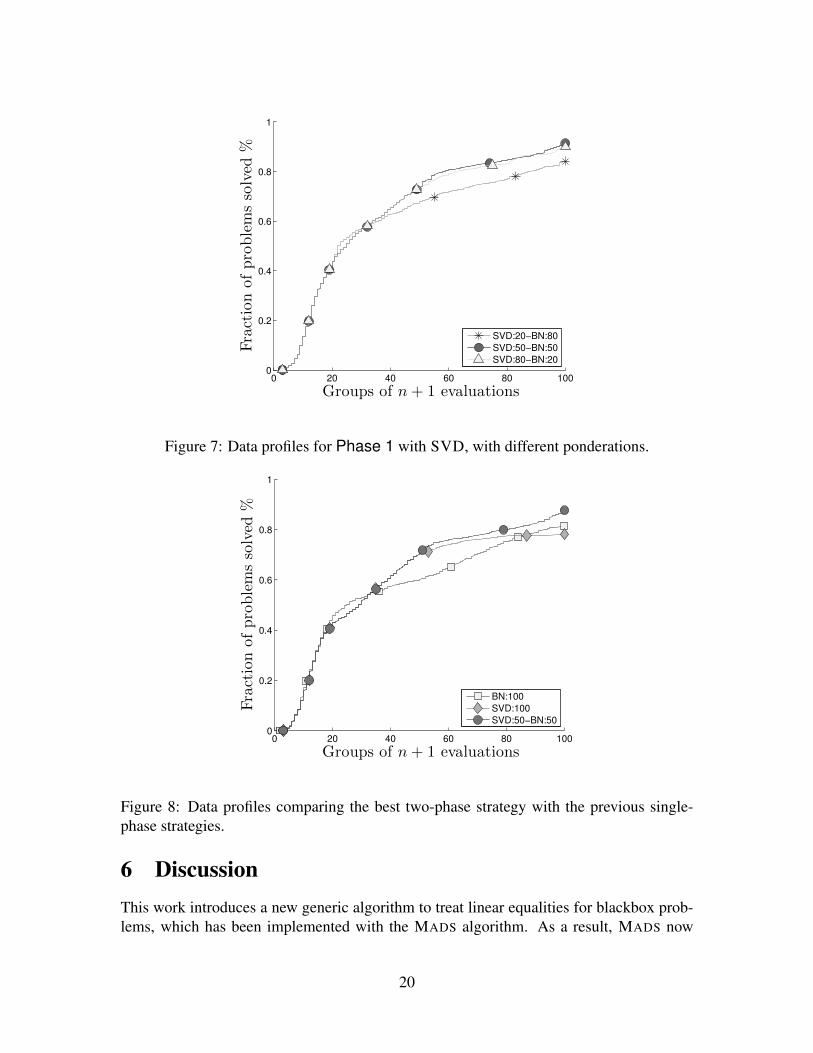
For Phase 1 using the SVD converter, different ponderations are compared in Fig-ure 7. These data profiles show that the best ponderation is 50–50. A too short Phase 1step is inefficient because it does not lead to a good choice of BN, while a longer Phase 1may waste evaluations.

The last comparison shown in Figure 8 is between the best two-phase strategy SVD:50-BN:50 and the previous best algorithms BN and SVD. We can conclude that SVD:50-BN:50 improves both algorithms.

These comparisons demonstrate that the two-phase strategy is effective, and this sug-gests that a new multi-phase algorithm involving more than two phases would be efficienttoo. We tested such a multi-phase algorithm, a four-phase repeating twice the two-phasealgorithm SVD:25–BN:25, but our results (not reported here) are not as good as expected.After analysis of these results, it appears that some changes of phase occurred too soon tobe efficient and that there were issues with the control of the scaling.

19

0 20 40 60 80 1000

0.2

0.4

0.6

0.8

1

Groups of n+ 1 evaluations

Fractionofproblemssolved

%

SVD:20−BN:80

SVD:50−BN:50

SVD:80−BN:20

Figure 7: Data profiles for Phase 1 with SVD, with different ponderations.

0 20 40 60 80 1000

0.2

0.4

0.6

0.8

1

Groups of n+ 1 evaluations

Fractionofproblemssolved

%

BN:100

SVD:100

SVD:50−BN:50

Figure 8: Data profiles comparing the best two-phase strategy with the previous single-phase strategies.

6 DiscussionThis work introduces a new generic algorithm to treat linear equalities for blackbox prob-lems, which has been implemented with the MADS algorithm. As a result, MADS now

20

possesses the ability to treat linear equalities, while preserving the convergence results thatthe Clarke derivative are nonnegative in the hyper tangent cone relative to the nullspaceof the constraint matrix. The proof relies on a theorical result showing that hypertangentcones are mapped by surjective linear application in finite dimension.

The best strategy identified by numerical results on a collection of 10 problems fromthe CUTEst collection consists to first use SVD to identify potentially active variables andthen to continue with BN to terminate the optimization process. This combines advantagesof both converters and is made possible thanks to a detailed analyse of the BN converter.Our results are similar to HOPSPACK for small to medium problems, but are better forthe larger instances.

Future work includes the integration of this new ability to the NOMAD software pack-age as well as its application to linear inequalities. In addition, the inexact restorationmethod of [6] could rely on the present work.

References[1] M.A. Abramson, C. Audet, J.E. Dennis, Jr., and S. Le Digabel. OrthoMADS: A deter-

ministic MADS instance with orthogonal directions. SIAM Journal on Optimization,20(2):948–966, 2009.

[2] M.A. Abramson, O.A. Brezhneva, J.E. Dennis Jr., and R.L. Pingel. Pattern search inthe presence of degenerate linear constraints. Optimization Methods and Software,23(3):297–319, 2008.

[3] C. Audet. A survey on direct search methods for blackbox optimization and their ap-plications. In P.M. Parardalos and T.M. Rassias, editors, Mathematics without bound-aries: Surveys in interdisciplinary research. Springer, 2014.

[4] C. Audet and J.E. Dennis, Jr. Mesh adaptive direct search algorithms for constrainedoptimization. SIAM Journal on Optimization, 17(1):188–217, 2006.

[5] C. Audet and J.E. Dennis, Jr. A progressive barrier for derivative-free nonlinearprogramming. SIAM Journal on Optimization, 20(1):445–472, 2009.

[6] L. Bueno, A. Friedlander, J. Martınez, and F. Sobral. Inexact restoration method forderivative-free optimization with smooth constraints. SIAM Journal on Optimization,23(2):1189–1213, 2013.

[7] A. Civril and M. Magdon-Ismail. On selecting a maximum volume sub-matrix of amatrix and related problems. Theoretical Computer Science, 410(47–49):4801–4811,2009.

[8] F.H. Clarke. Optimization and Nonsmooth Analysis. John Wiley & Sons, New York,1983. Reissued in 1990 by SIAM Publications, Philadelphia, as Vol. 5 in the seriesClassics in Applied Mathematics.

21

[9] A.R. Conn, N.I.M. Gould, and Ph.L. Toint. A globally convergent augmented La-grangian algorithm for optimization with general constraints and simple bounds.SIAM Journal on Numerical Analysis, 28(2):545–572, 1991.

[10] A.R. Conn, K. Scheinberg, and Ph.L. Toint. A derivative free optimization algorithmin practice. In Proceedings the of 7th AIAA/USAF/NASA/ISSMO Symposium on Mul-tidisciplinary Analysis and Optimization, St. Louis, Missouri, 1998.

[11] A.R. Conn, K. Scheinberg, and L.N. Vicente. Introduction to Derivative-Free Opti-mization. MOS/SIAM Series on Optimization. SIAM, Philadelphia, 2009.

[12] I.D. Coope and C.J. Price. On the convergence of grid-based methods for uncon-strained optimization. SIAM Journal on Optimization, 11(4):859–869, 2001.

[13] N.I.M. Gould, D. Orban, and Ph.L. Toint. CUTEst: a constrained and unconstrainedtesting environment with safe threads. Technical Report G-2013-27, Les cahiers duGERAD, 2013.

[14] J.D. Griffin, T.G. Kolda, and R.M. Lewis. Asynchronous parallel generating setsearch for linearly-constrained optimization. SIAM Journal on Scientific Computing,30(4):1892–1924, 2008.

[15] W. Hock and K. Schittkowski. Test Examples for Nonlinear Programming Codes,volume 187 of Lecture Notes in Economics and Mathematical Systems. SpringerVerlag, Berlin, Germany, 1981.

[16] B. Ivanov, A. Galushko, and R. Stateva. Phase stability analysis with equations ofstate – a fresh look from a different perspective. Industrial & Engineering ChemistryResearch, 52(32):11208–11223, 2013.

[17] J. Jahn. Introduction to the theory of nonlinear optimization. Springer, third edition,2007.

[18] T.G. Kolda, R.M. Lewis, and V. Torczon. A generating set direct search augmentedLagrangian algorithm for optimization with a combination of general and linear con-straints. Technical Report SAND2006-5315, Sandia National Laboratories, USA,2006.

[19] T.G. Kolda, R.M. Lewis, and V. Torczon. Stationarity results for generating set searchfor linearly constrained optimization. SIAM Journal on Optimization, 17(4):943–968,2006.

[20] R.M. Lewis, A. Shepherd, and V. Torczon. Implementing generating set search meth-ods for linearly constrained optimization. SIAM Journal on Scientific Computing,29(6):2507–2530, 2007.

[21] R.M. Lewis and V. Torczon. Pattern search methods for linearly constrained mini-mization. SIAM Journal on Optimization, 10(3):917–941, 2000.

22

[22] R.M. Lewis and V. Torczon. Active set identification for linearly constrained min-imization without explicit derivatives. SIAM Journal on Optimization, 20(3):1378–1405, 2010.

[23] R.M. Lewis and V. Torczon. A direct search approach to nonlinear programmingproblems using an augmented lagrangian method with explicit treatment of linearconstraints. Technical report, College of William & Mary, 2010.

[24] L. Liu and X. Zhang. Generalized pattern search methods for linearly equality con-strained optimization problems. Applied Mathematics and Computation, 181(1):527–535, 2006.

[25] J.H. May. Linearly Constrained Nonlinear Programming: A Solution Method ThatDoes Not Require Analytic Derivatives. PhD thesis, Yale University, December 1974.

[26] R. Mifflin. A superlinearly convergent algorithm for minimization without evaluatingderivatives. Mathematical Programming, 9(1):100–117, 1975.

[27] J.J. More and S.M. Wild. Benchmarking derivative-free optimization algorithms.SIAM Journal on Optimization, 20(1):172–191, 2009.

[28] J. Nocedal and S.J. Wright. Numerical Optimization. Springer Series in OperationsResearch. Springer, New York, 1999.

[29] T.D Plantenga. HOPSPACK 2.0 user manual. Technical Report SAND2009-6265,Sandia National Laboratories, Livermore, CA, October 2009.

[30] M.J.D. Powell. Lincoa software. Software available at http://mat.uc.pt/˜zhang/software.html#lincoa.

[31] C.J. Price and I.D. Coope. Frames and grids in unconstrained and linearly constrainedoptimization: A nonsmooth approach. SIAM Journal on Optimization, 14(2):415–438, 2003.

[32] W. Rudin. Functional analysis. International Series in Pure and Applied Mathemat-ics. McGraw-Hill Inc., New York, second edition, 1991.

[33] V. Torczon. On the convergence of pattern search algorithms. SIAM Journal onOptimization, 7(1):1–25, 1997.

23