Linear Finite Transducers Towards a Public Key ... · Linear Finite Transducers Towards a Public...

Linear Finite Transducers Towards a Public Key Cryptographic System

Ivone de Fátima da Cruz Amorim Tese de Doutoramento apresentada à Faculdade de Ciências da Universidade do Porto, Ciência de Computadores

2016

D

D

!Linear Finite Transducers Towards a Public Key Cryptographic System

Ivone de Fátima da Cruz Amorim Doutoramento em Ciência de Computadores Departamento de Ciência de Computadores 2016 Orientador Rogério Ventura Lages dos Santos Reis, Professor Auxiliar, Faculdade de Ciências da Universidade do Porto. Coorientador António José de Oliveira Machiavelo, Professor Auxiliar, Faculdade de Ciências da Universidade do Porto.

To my father, who taught me the true meaning of courage.

Ao meu pai, por me ensinar o verdadeiro significado da palavra coragem.

v

vi

Acknowledgments

I would like to take this opportunity to express my gratitude to a few people that

supported me throughout the course of this project. First of all, I would like to

acknowledge my supervisors, António Machiavelo and Rogério Reis, for their uncon-

ditional support from the beginning of this adventure. I thank them for the long

hours they spent with me, which went far beyond what I could demand, for all the

wise opinions they gave me about my work (and not only about the work), for all the

questions they raised, which were fundamental for my growth as a researcher, for their

(almost) infinite patience with my doubts and insecurities, and, finally, for the sense

of humor that was always present in our meetings. I will always be grateful to them.

To Professor Renji Tao I thank the celerity with which he has always replied to my

emails, and I also thank him for sending me a copy of documents that otherwise would

be almost impossible to obtain.

I thank Professor Stavros Konstantidinis for his invitation to spend a month in Saint

Mary’s University as a visiting scholar. I also thank him for his kindness, hospitality

and for all the scientific discussions I was able to have during my stay in Halifax.

To Nelma Moreira I thank for being always available when I needed her. I also thank

her, and Rogério, for hosting me in the house they rented in Halifax, for the availability

and care they always showed, and for all the exploring trips and conversations we had

during my stay.

To Alexandra and Isabel for being always so efficient and helpful with all the bureau-

vii

cratic questions, and for the good moments we shared during our "knitting meetings".

To my colleagues in general for their constant encouragement. To Cristina Lima for

her prompt availability to proofread some parts of this thesis. A very special thanks

goes to Eva Maia, with whom I shared much more than an office during my PhD. I

thank her for all the conversations we had on the most diverse subjects, for all the

opinions she gave me, always with different points of view, for the patience she showed

to listen to my problems, even when she also needed support, and, mostly, for the

moments we laughed together when we just wanted to cry.

To my siblings, Elisa, Fernando and Rui, for all the care over the years, for their

encouragement, and for tolerating my bad mood in complicated moments. To my

stepmother for the fundamental values she taught me. To my nieces and nephews,

Beatriz, Bianca, Celia, Simão and Javier, I thank for all the moments we played

together, which brought a lot of happiness to my life. To my sisters in law, Susete and

Cristina, I thank for all the conversations and for always being so supportive.

I thank Paulo for the care and comprehension with which he always dealt with my

absences, for listening to me and for the encouragement he gave me when I was

questioning myself, for believing in my work, and for helping me to focus in what

was important in the last phase of this journey.

Finally, I thank my father to whom I own the basis of my education. I thank him for

always giving me the freedom to choose my way, for stimulating my critical spirit, and

for showing me, through his own example, that we can make our dreams come true.

Above all, I thank him for making the well-being of our family his priority, when we

most needed him.

Regarding financial support, I thank Fundação para a Ciência e Tecnologia for the

PhD grant [SFRH/BD/84901/2012], and to Centro de Matemática da Universidade

do Porto for funding all my conference participations.

viii

Agradecimentos

Aproveito esta oportunidade para fazer um pequeno agradecimento a algumas pessoas

que me apoiaram ao longo deste trabalho. Em primeiro lugar, quero agradecer aos

meus orientadores, António Machiavelo e Rogério Reis, pelo apoio incondicional desde

o início desta aventura. Agradeço pelas longas horas que me dispensaram, que foram

muito além do que eu poderia exigir, por todas as opiniões sábias que deram sobre o

meu trabalho (e não só), por todas as questões que colocaram, que foram fundamentais

no meu crescimento enquanto investigadora, pela sua (quase) infinita paciência para as

minhas dúvidas e inseguranças e, finalmente, pelo sentido de humor que esteve sempre

presente nas nossas reuniões.

Ao Professor Renji Tao agradeço a rapidez com que sempre respondeu aos meus emails

e por tão prontamente me ter disponibilizado documentos que de outra forma eu

dificilmente conseguiria obter.

Agradeço ao Professor Stavros Konstantinidis pelo convite para passar um período na

Saint Mary’s University na qualidade de visiting scholar. Agradeço, ainda, pela sua

simpatia, hospitalidade e por todas as discussões científicas em que pude participar

durante a minha estadia em Halifax.

À Nelma Moreira agradeço toda a disponibilidade que sempre demonstrou nas mais

diversas situações em que precisei da sua ajuda. Agradeço-lhe, ainda, tal como

agradeço ao Rogério, por me terem acolhido na casa que alugaram em Halifax, pela

disponibilidade e preocupação que sempre demonstraram e por todos os passeios e

conversas que tivemos durante a minha estadia.

ix

Agradeço à Alexandra e à Isabel por tão eficientemente me terem ajudado na resolução

de todas as questões burocráticas que foram surgindo e por todos os bons momentos

que partilhamos durante as nossas "reuniões do tricô".

Agradeço a todos os meus colegas que, de alguma forma, me incentivaram. À Cristina

Lima por se ter disponibilizado tão prontamente a ler partes desta tese e por ter

estado sempre disponível para me ouvir. Deixo um agradecimento muito especial

à Eva Maia, com quem partilhei muito mais do que um gabinete durante o meu

doutoramento. Agradeço-lhe pelas nossas conversas sobre os mais diversos assuntos,

por todas as opiniões que me deu com pontos de vista sempre diferentes, pela paciência

com que ouviu os meus desabafos mesmo quando ela também precisava de apoio e,

principalmente, por todos os momentos em que nos rimos, quando só nos apetecia

chorar.

Agradeço aos meus irmãos, Elisa, Fernando e Rui, por todo o carinho que me deram

ao longo da minha vida, por me incentivarem e por tolerarem o meu mau humor

em momentos mais complicados. À minha madrasta, agradeço pelos valores funda-

mentais que me transmitiu. Aos meus sobrinhos, Simão, Beatriz, Bianca, Celia e

Javier, agradeço por todas as travessuras e momentos de brincadeira que partilhamos,

momentos esses que tornaram a minha vida muito mais feliz. Às minhas cunhadas,

Susete e Cristina, agradeço por todas as conversas que tivemos e por sempre me terem

apoiado.

Agradeço ao Paulo pelo carinho e pela compreensão com que sempre lidou com as

minhas ausências. Por me ter ouvido e incentivado nas imensas vezes em que duvidei

de mim. Por ter acreditado no meu trabalho e por me ter ajudado a focar naquilo que

era importante na fase final deste percurso.

Por fim, agradeço ao meu pai, a quem devo a base da minha educação. Agradeço-lhe

por sempre me ter dado a liberdade de escolher o meu caminho, por ter estimulado

o meu espírito crítico e por me ter mostrado, através do seu próprio exemplo, que é

possível concretizarmos os nossos sonhos. Acima de tudo, agradeço-lhe por ter feito

x

do bem-estar da nossa família a sua prioridade quando mais precisamos.

No que diz respeito ao suporte financeiro, agradeço à Fundação para a Ciência e Tec-

nologia pela bolsa de doutoramento [SFRH/BD/84901/2012] e ao Centro de Matemática

da Universidade do Porto por financiar todas as despesas inerentes às minhas deslo-

cações às várias conferências.

xi

xii

Abstract

Cryptography faces a set of new challenges. The rapid advance in computing power and

technology, as well as the possibility of quantum computing becoming a reality, are real

threats to the security offered by classical cryptographic systems. New cryptographic

systems, relying in different assumptions, are needed.

Cryptographic systems based on finite transducers are an exciting possible solution to

these new challenges. First, their security does not rely on complexity assumptions

related to number theory problems (as classical systems do), it relies on the apparent

difficulties of inversion of non-linear finite transducers and of factoring matrix polyno-

mials over Fq. Secondly, they offer relatively small key sizes as well as linear encryption

and decryption times complexity.

The techniques used in these systems depend heavily on the results of invertibility of

linear finite transducers (LFTs). In this thesis we give a complete characterisation of

LFTs, while discussing their invertibility. A wide variety of examples are presented in

order to illustrate the concepts and techniques proposed.

The main original contributions of this work are the following.

• An equivalence test for LFTs.

• A canonical representation for LFTs, and an algorithm to compute such a

representation.

• Methods to compute the number and size of equivalence classes of LFTs defined

xiii

over Fq, and an algorithm to enumerate all the equivalent LFTs with the same

number of states.

• The implementation of an algorithm that employees a known condition, due to

Zongduo and Dingfeng, to check ⌧ -injectivity of LFTs.

• Methods to estimate the number and percentage of ⌧ -injective equivalence classes

(⌧ 2 N0), by uniform random generation of LFTs, and implementations of these

methods in Python using some Sage modules to deal with matrices.

• An experimental study using these implementations.

• An extension of the concept of LFT with memory, called PILT, and a necessary

and sufficient condition for the injectivity of these transducers.

• An algorithm to invert PILTs, which, since LFTs with memory are PILTs, allows

to find left inverses of invertible LFTs with memory.

xiv

Resumo

A Criptografia enfrenta um conjunto de novos desafios. A rápida evolução da tecnolo-

gia e do poder computacional, assim como a possibilidade da computação quântica

se tornar uma realidade, são ameaças sérias à segurança oferecida pelos sistemas

criptográficos clássicos. São necessários novos sistemas criptográficos que assentem

em diferentes pressupostos de complexidade.

Os sistemas criptográficos baseados em transdutores finitos são uma possível solução

para estes novos desafios. Em primeiro lugar, a sua segurança não assenta em pressu-

postos de complexidade relacionados com problemas de teoria de números (tal como

os sistemas clássicos), mas sim na dificuldade da inversão de transdutores finitos não

lineares e na dificuldade da factorização de matrizes polinomiais. Por outro lado,

os tamanhos da chave exigidos são relativamente pequenos e os tempos de cifra e

decifração são lineares.

As técnicas usadas nestes sistemas dependem fortemente dos resultados existentes

sobre a invertibilidade de transdutores finitos lineares (TFLs). Nesta tese dá-se uma

caracterização completa destes transdutores e, ao mesmo tempo, discute-se a sua

invertibilidade. Além disso, também é apresentada uma grande variedade de exemplos

que permitem ilustrar os conceitos e técnicas aqui propostos.

As principais contribuições originais deste trabalho são as seguintes.

• Um teste que permite verificar a equivalência de TFLs.

• Uma representação canónica para TFLs e um algoritmo para determinar essa

xv

representação.

• Métodos para calcular o número e o tamanho das classes de equivalência de

TFLs definidos sobre Fq e um algoritmo que permite enumerar todos os TFLs

equivalentes que têm o mesmo número de estados.

• A implementação de um algoritmo que aplica uma condição já conhecida para

verificar se um TFL é ⌧ -injectivo.

• Métodos para estimar o número e a percentagem de classes de equivalência ⌧ -

injectivas, usando geração aleatória uniforme de TFLs, e implementações destes

métodos em Python usando alguns módulos do Sage para trabalhar com ma-

trizes.

• Um estudo experimental usando estas implementações.

• Uma extensão do conceito de TFL com memória, chamada PILT, e uma condição

necessária e suficiente para a injectividade destes transdutores.

• Um algoritmo para inverter PILTs que, uma vez que os TFLs com memória são

PILTs, permite encontrar um inverso à esquerda de qualquer TFL com memória

que seja injectivo.

xvi

Resumé

La Cryptographie est aujourd’hui devant des nouveaux défis. L’avance rapide de la

puissance de calcul des ordinateurs et de la technologie, ainsi que la possibilité des ordi-

nateurs quantiques devient une réalité, sont de sérieux menaces à la sécurité offerte par

des systèmes cryptographiques classiques. Des nouveaux systèmes cryptographiques en

se fondant dans différentes hypothèses de complexité sont donc nécessaires.

Les systèmes cryptographiques édifiés sur les transducteurs finis constitue une solution

prometteuse à ces nouveaux défis. Tout d’abord, leur sécurité ne repose pas dans les

hypothèses de la complexité des problèmes liés à la théorie des nombres (comme pour

les systèmes classiques), elle repose sur les apparentes difficultés de l’inversion des

automates finis non linéaires et de la factorisation des polynômes matriciels sur Fq.

Deuxièmement, ils offrent des clés à tailles relativement petites, ainsi qu’une chiffrage

et le déchiffrage à temps linéaire.

Les techniques utilisées dans ces systèmes dépendent fortement des résultats de l’in-

versibilité de transducteurs finis linéaires (TFLs). Dans cette thèse, on donne une

caractérisation complète de TFLs et on discute de leur inversibilité. Des différent

exemples sont données pour illustrer les concepts et les techniques proposées.

Les principales contributions originales de ce travail sont les suivants :

• Un algoritme pour tester l’équivalence de TFLs.

• Une représentation canonique pour TFL et un algorithme pour calculer cette

représentation.

xvii

• Méthodes pour calculer le nombre d’éléments et la taille des classes d’équiva-

lence de transducteurs finis définies sur Fq qui sont ⌧ -injective (⌧ 2 N0), et un

algorithme pour énumérer tous les TFLs équivalentes qui ont le même nombre

d’états.

• La implémentation d’un algorithme en utilisant une condition de Zongduo et

Dingfeng pour vérifier la ⌧ -injectivité de TFLs.

• Méthodes pour estimer le nombre et le pourcentage de classes d’équivalence qui

sont ⌧ -injective, pour génération aléatoire uniforme de TFLs, et des implémen-

tations de ces méthodes en Python utilisant certains modules de Sage pour le

traitement des matrices.

• Une étude expérimentale utilisant ces implémentations.

• Une extension de la notion de TFL avec mémoire, que nous avons appelé PILT,

et une condition nécessaire et suffisante pour l’injectivité de ces transducteurs.

• Un algorithme pour inverser PILTs, qui, une fois que les TFLs avec mémoire

sont PILTs, permet de trouver inverses gauche des TFLs avec mémoire qui sont

inversibles.

xviii

Contents

Acknowledgments vii

Agradecimentos ix

Abstract xiii

Resumo xv

Resumé xvii

List of Tables xxiii

List of Figures xxv

List of Algorithms xxvii

1 Introduction 1

1.1 Structure of this Dissertation . . . . . . . . . . . . . . . . . . . . . . . 5

2 Mathematical Prerequisites 7

2.1 Relations and Funtions . . . . . . . . . . . . . . . . . . . . . . . . . . . 7

xix

2.2 Groups, Rings, PIDs, and Fields . . . . . . . . . . . . . . . . . . . . . . 9

2.3 Modules and Vector Spaces . . . . . . . . . . . . . . . . . . . . . . . . 14

2.4 Matrices and Smith Normal Form . . . . . . . . . . . . . . . . . . . . . 16

2.5 Cayley-Hamilton Theorem and Some Implications . . . . . . . . . . . . 25

2.6 Linear Maps . . . . . . . . . . . . . . . . . . . . . . . . . . . . . . . . . 27

3 Linear Finite Transducers 31

3.1 Preliminaries on Finite Transducers . . . . . . . . . . . . . . . . . . . . 31

3.1.1 Concepts on Invertibility . . . . . . . . . . . . . . . . . . . . . . 43

3.1.2 Finite Transducers with Memory . . . . . . . . . . . . . . . . . 48

3.2 The Notion of Linear Finite Transducer . . . . . . . . . . . . . . . . . . 51

3.3 Equivalence of States and of LFTs . . . . . . . . . . . . . . . . . . . . 54

3.4 Minimisation . . . . . . . . . . . . . . . . . . . . . . . . . . . . . . . . 61

4 Size and Number of Equivalence Classes of LFTs 65

4.1 Canonical Linear Finite Transducers . . . . . . . . . . . . . . . . . . . 65

4.2 Size of Equivalence Classes . . . . . . . . . . . . . . . . . . . . . . . . . 69

4.3 Number of Equivalence Classes . . . . . . . . . . . . . . . . . . . . . . 76

5 Equivalence Classes of Injective LFTs 81

5.1 Injectivity of LFTs . . . . . . . . . . . . . . . . . . . . . . . . . . . . . 81

5.2 Number of Injective Equivalence Classes . . . . . . . . . . . . . . . . . 88

5.3 Percentage of Injective Equivalence Classes . . . . . . . . . . . . . . . . 92

xx

5.4 Experimental Results . . . . . . . . . . . . . . . . . . . . . . . . . . . . 95

6 Inverses of LFTs with Memory 101

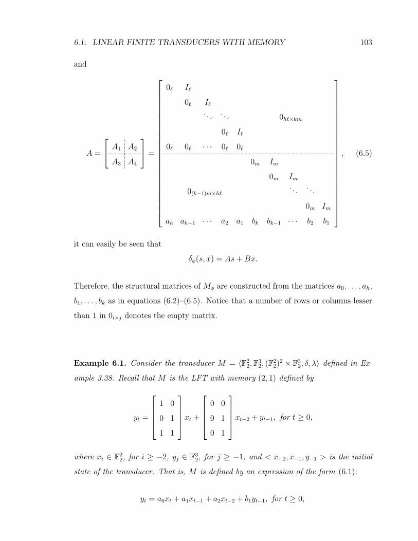
6.1 Linear Finite Transducers with Memory . . . . . . . . . . . . . . . . . 101

6.2 Injectivity of LFTs with Memory . . . . . . . . . . . . . . . . . . . . . 104

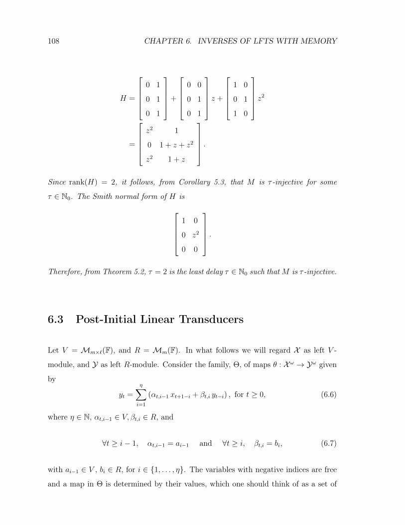
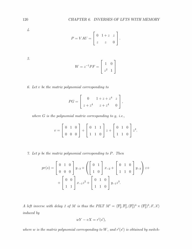
6.3 Post-Initial Linear Transducers . . . . . . . . . . . . . . . . . . . . . . 108

7 Conclusion 125

A Tables of Experimental Results 129

B Change of Variables in Summations 131

Index 136

xxi

xxii

List of Tables

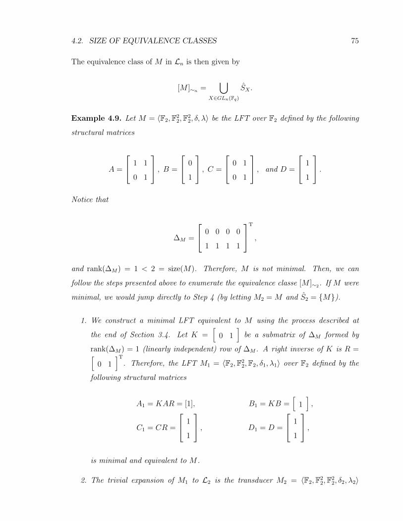
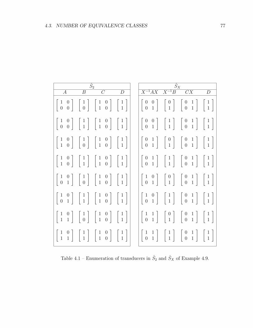
4.1 Enumeration of transducers in ˆS2 and ˆSX of Example 4.9. . . . . . . . 77

5.1 Approximated values for the number of injective equivalence classes

when m = 5 and ⌧ = 10. . . . . . . . . . . . . . . . . . . . . . . . . . . 95

6.1 Coefficients of ⇥. . . . . . . . . . . . . . . . . . . . . . . . . . . . . . . 109

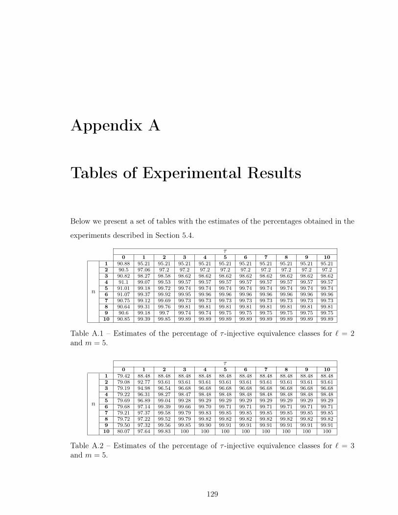
A.1 Estimates of the percentage of ⌧ -injective equivalence classes for ` = 2

and m = 5. . . . . . . . . . . . . . . . . . . . . . . . . . . . . . . . . . 129


and m = 5. . . . . . . . . . . . . . . . . . . . . . . . . . . . . . . . . . 129


and m = 5. . . . . . . . . . . . . . . . . . . . . . . . . . . . . . . . . . 130


and m = 5. . . . . . . . . . . . . . . . . . . . . . . . . . . . . . . . . . 130


and m = 8. . . . . . . . . . . . . . . . . . . . . . . . . . . . . . . . . . 130

xxiii

xxiv

List of Figures

5.1 Variation on the percentage of ⌧ -injective equivalence classes for ` = 2,

m = 5, and several values of n and ⌧ (from two different perspectives). 96

5.2 Variation on the percentage of ⌧ -injective equivalence classes for m = 5

and several values of `, n and ⌧ . . . . . . . . . . . . . . . . . . . . . . . 97

5.3 Variation on the percentage of ⌧ -injective equivalence classes for m = 5

and several values of `, n and ⌧ (from a different perspective than that

from Figure 5.2). . . . . . . . . . . . . . . . . . . . . . . . . . . . . . . 98

5.4 Variation on the percentage of ⌧ -injective equivalence classes for ` = 8,

m = 8, and several values of n and ⌧ (from two different perspectives). 99

xxv

xxvi

List of Algorithms

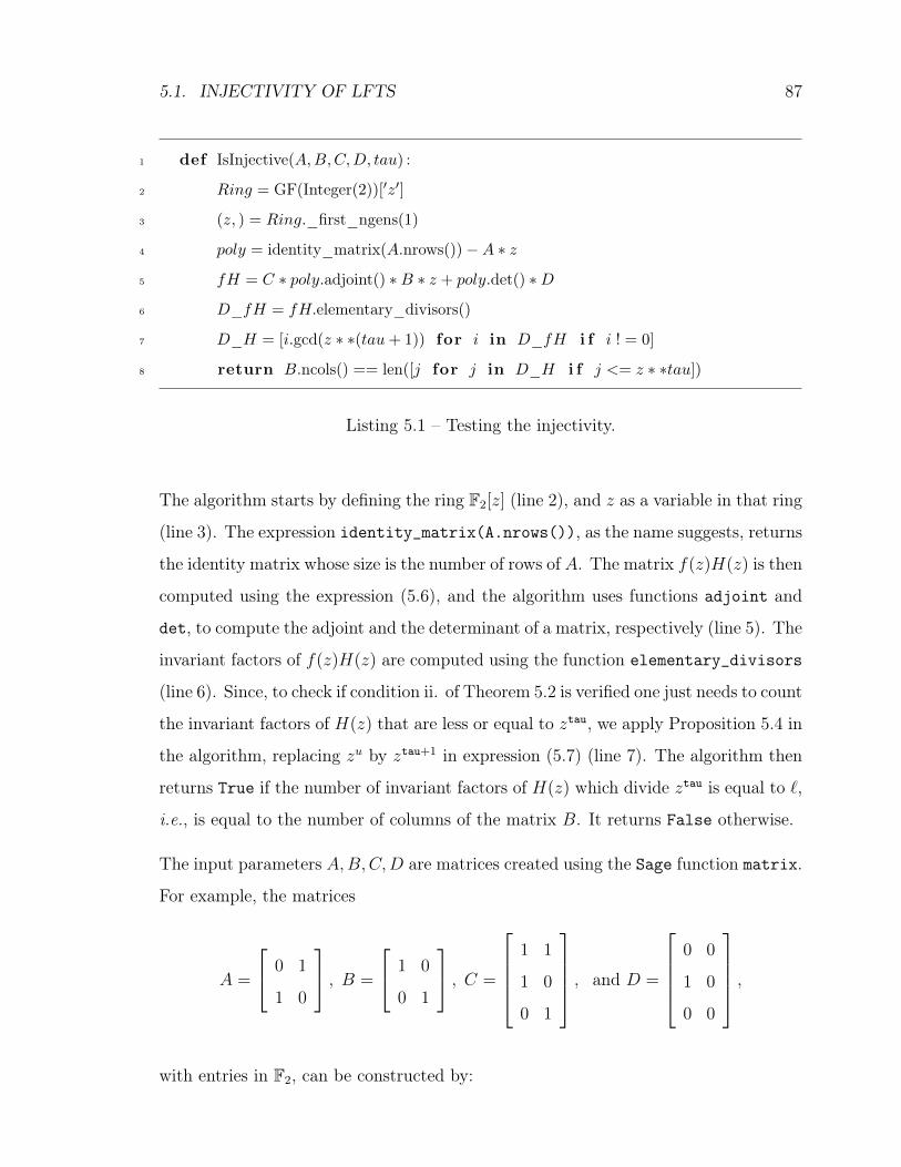
5.1 Testing the injectivity. . . . . . . . . . . . . . . . . . . . . . . . . . . . 87

5.2 Determining the size of equivalence classes. . . . . . . . . . . . . . . . . 90

5.3 Estimating the number of non-equivalent LFTs. . . . . . . . . . . . . . 91

5.4 Auxiliary functions. . . . . . . . . . . . . . . . . . . . . . . . . . . . . . 92

5.5 Counting the number of canonical LFTs. . . . . . . . . . . . . . . . . . 93

5.6 Estimating the percentage of injective equivalence classes. . . . . . . . . 94

xxvii

xxviii

Chapter 1

Introduction

The concept of Public Key Cryptography (PKC) was introduced by Diffie, Hellman

and Merkle in 1976. In 1978, Rivest, Shamir and Adleman presented the first public

key cryptosystem, called RSA [Dif88]. The RSA system, and most of the public

key cryptosystems created in the following years, are based on complexity assump-

tions related to number theory problems, namely the factorisation of integers and

the discrete logarithm problem. This dependence on a very small set of problems

makes such cryptosystems somewhat vulnerable. Also, improvements in algorithms

to solve these problems have led to the need of increasing the size of the keys, which

implies higher computational costs. Moreover, the past few years have witnessed an

astonishing increase on the diversity of small computing devices allowing to implement

almost every kind of digital service that, up to now, were only possible on computers.

These small devices are very attractive, and are now affordable by almost everyone.

However, they have very limited resources, which requires new cryptographic solutions

that should be both secure and extremely fast.

In a series of papers [TC85, TCC97, TC97, TC99], Renji Tao introduced a family of

cryptosystems based on finite transducers, named FAPKCs (which stands for Finite

Automata Public Key Cryptosystems), which seems to be a good alternative to the

classical ones. First, the security of these systems does not rely on complexity as-

1

2 CHAPTER 1. INTRODUCTION

sumptions related to number theory problems (as classical systems do), rather relying

on the difficulty of inverting non-linear finite transducers and of factoring matrix

polynomials over Fq [Tao09]. The complexity of these problems is not known, apart

from the trivial fact that they are both NP-problems, exactly like the integer factoring

problem that is the basis of RSA. Secondly, they offer relatively small key sizes as well

as fast encryption and decryption [TC97, Abu11]. This makes them computationally

attractive, and thus suitable for application on devices with very limited computational

resources, such as satellites, cellular phones, sensor networks, and smart cards [TC97].

Besides, the FAPKC schemes are stream ciphers that can be used for encryption and

signature [Tao09].

The first FAPKC system was proposed in 1985 by Tao and Chen in a paper (in Chinese)

and was named FAPKC0. An English description of it was presented in a later work of

the same authors [TC86]. Roughly speaking, in this system, the private key consists of

two injective transducers with memory, where one is a linear finite transducer (LFT),

M , and the other is a non-linear finite transducer (non-LFT), N , whose left inverses

can be easily computed. The public key is the result of applying a special product for

transducers, C, to the original pair, thus obtaining a non-LFT, denoted by C(M,N).

The crucial point is that it is easy to obtain an inverse of C(M,N) from the inverses of

its factors, M�1 and N�1, while it is believed to be hard to find that inverse without

knowing those factors. On the other hand, the factorisation of a transducer seems to

be hard by itself [ZDL98].

The system FAPKC0 was derived mainly from the results about invertibility on LFTs

presented by Tao in 1973 [Tao73], which was the first relevant work on invertibility

theory of finite transducers with applications to Cryptography. In 1986, Tao and

Chen published two variants of that cryptosystem, named FAPKC1 and FAPKC2

[TC86], but with no further advances on the invertibility theory of finite transducers.

In 1992, the methods used to study the invertibility of LFTs were applied to quasi-

linear finite transducers over finite fields (as defined by Tao [Tao09]). And, in 1995,

they were generalised to construct pairs of transducers in which one is a left inverse

3

of the other. This new development on the invertibility theory of finite transducers

gave rise to two new cryptographic schemes: FAPKC3 and FAPKC4, presented by Tao

et al. [TCC97] and by Tao and Chen [TC97], respectively. Meanwhile, some other

schemes of Public Key Cryptography based on finite transducers were developed (the

system FAPKC93 was presented in a PhD thesis written in Chinese, and a variant

of FAPKC2 was put forward by Bao and Igarashi [BI95]). All of these systems are

similar in structure, their main difference being the choice of the transducers for the

private key. For example, while in the FAPKC0 system M is linear and N is non-

linear, in the system FAPKC3 the transducers M and N are both non-linear. The

systems FAPKC0, FAPKC1, FAPKC93 and the variant of FAPKC2, were proved to

be insecure [Tao95a, Tao95b, TC97]. The systems FAPKC2, FAPKC3 and FAPKC4

have not yet been adequately evaluated.

Although some of the FAPKC schemes were already shown to be insecure, the promise

of a new system of PKC relying on different complexity assumptions makes these

systems worth exploring. However, the uninspiring and arid language used in Tao’s

works seems to have condemned these systems to oblivion. Moreover, the study of finite

transducers and their invertibility is spread over a series of papers that sometimes do

not contain proofs, or refer to papers that are written in Chinese and/or are not easily

available to the English reader. Also, there is an almost total lack of examples, making

it difficult to understand the underlying theory. From all this, it is clear that, on the

one hand, there is a need for a clarification and consolidation of the work already done

in this subject and, on the other hand, it is necessary to do a serious study of these

systems and their application. This thesis is a starting point in that direction.

In this work, we give an unified presentation of the known results, as far as we can

establish, on general linear finite transducers as well as on linear transducers with

memory. We also simplify the language used, by introducing a more classical point of

view.

As our first contribution we present a new equivalence test for LFTs which is of

paramount importance in the following work. We then give a complete characterisation


of these transducers, by introducing a notion of canonical LFT and by studying the

number and size of LFT’s equivalence classes. An algorithm to enumerate the LFTs

in the same equivalence class is also provided.

We then show how to estimate the number and percentage of non-equivalent LFTs

that are ⌧ -injective (⌧ 2 N0), by uniform random generation of LFTs. This number is

fundamental to evaluate the key space of cryptographic systems that use this kind of

transducers, and their percentage is crucial to conclude if uniform random generation

of non-equivalent LFTs is a feasible option to generate cryptographic keys. As far

as we know, no similar study has ever been conducted. All the algorithms presented

were implemented in Python using some Sage [Dev15] modules to deal with matrices.

Several experiments were carried out and the results obtained are also given, which

by themselves constitute an important step towards the evaluation of these systems.

Finally, we address the invertibility problem in LFTs with memory. Inverting transduc-

ers of this kind is fundamental in the key generation process of FAPKCs that use LFTs,

since one needs to define both an invertible LFT with memory and a corresponding

left inverse. Moreover, new techniques to invert injective finite transducers may allow

to study the vulnerability of the existent cryptographic systems from novel points

of view. Despite the works done on the invertibility of LFTs [Tao73, Tao88, ZD96,

ZDL98, HZ99], none of them presents an algorithm to invert LFTs with memory. Thus,

in this work, we introduce the notion of post-initial linear transducer (PILT), which

is an extension of the notion of LFT with memory, and give explicitly an algorithm to

invert this kind of transducers.

We also present, throughout this work, a wide variety of examples to illustrate the

concepts and techniques proposed.

1.1. STRUCTURE OF THIS DISSERTATION 5

1.1 Structure of this Dissertation

We start by reviewing, in Chapter 2, several concepts and some results from different

areas of mathematics that will be used throughout this work. We also introduce some

convenient notation.

Preliminary notions and results of general finite transducers are given in Chapter 3,

including the concepts of injectivity and invertibility that are considered in this work.

Also, in this chapter, we give the definition of LFT, present some already known

results, and give our new method to check LFT’s equivalence. At the end, we discuss

the minimisation problem of these transducers.

In Chapter 4, we give our notion of canonical LFT and prove that each equivalence

class has exactly one of these transducers. We also show how to construct the

canonical LFT equivalent to an LFT given in its matricial form. Then, by using the

new equivalence test for LFTs presented in Chapter 3, we enumerate and count the

equivalent transducers with the same size. From this, we derive a recurrence relation

that counts the number of equivalence classes, i.e., the number of non-equivalent LFTs.

Chapter 5 is devoted to the statistical study on the number and percentage of ⌧ -

injective equivalence classes. We start by reviewing some results on the invertibility of

LFTs and by giving an algorithm to test if an LFT is injective with some delay ⌧ 2 N0.

Then, we show how to estimate the number of ⌧ -injective equivalence classes, using

the results of the previous chapter about the size of equivalence classes. After that, we

deal with the problem of computing the percentage of ⌧ -injective equivalence classes,

using the estimate for the number of those classes and the fact that each equivalence

class has exactly one canonical LFT. We end this chapter with a presentation and

discussion of our experimental results.

The invertibility problem in LFTs with memory is dealt with in Chapter 6. We first

discuss the form of the structural matrices for LFTs with memory, and then we study

how that form allows to simplify the method presented in the previous chapter to check


injectivity of LFTs. The notion of PILT is then introduced as well as the method we

propose to compute left inverses of invertible PILTs. Since an LFT with memory is

also a PILT, this method allows to invert any injective LFT with memory.

Finally, in Chapter 7, we summarise our contributions and discuss some future research

directions.

Some of the results here included were previously presented in conferences of the area

or published in scientific journals [AMR14a, AMR14c, AMR15, AMR12, AMR14b].

Chapter 2

Mathematical Prerequisites

2.1 Relations and Funtions

Let A and B be two sets. A relation ⇠ from A to B is a subset of the cartesian product

A⇥B. We write a ⇠ b to denote that (a, b) is in the relation ⇠. If (a, b) is not in the

relation ⇠, we write a 6⇠ b. When A = B, ⇠ is also called a binary relation on A.

A binary relation ⇠ on a set A is said to be an equivalence relation if and only if the

following conditions hold:

• ⇠ is reflexive, i.e., a ⇠ a, for all a in A;

• ⇠ is symmetric, i.e., a ⇠ b if and only if b ⇠ a, for all a, b in A;

• ⇠ is transitive, i.e., if a ⇠ b and b ⇠ c, then a ⇠ c, for all a, b, c in A.

Let ⇠ be an equivalence relation on A. For any a 2 A, the set [a]⇠ = {b 2 A | a ⇠ b}

is called the equivalence class containing a, while the set of all equivalence classes,

A/⇠ = {[a]⇠ | a 2 A}, is called the quotient of A by ⇠.

The restriction of a binary relation on a set A to a subset S is the set of all pairs (a, b)

in the relation for which a and b are in S. If a relation is an equivalence relation, its

7

8 CHAPTER 2. MATHEMATICAL PREREQUISITES

restrictions are too.

Given a positive integer n, an example of an equivalence relation is the congruence

modulo n relation on the set of integers, Z. For a positive integer n, one defines this

relation on Z as follows. Two integers a and b are said to be congruent modulo n,

written:

a ⌘n b or a ⌘ b (mod n),

if their difference a� b is a multiple of n. It is easy to verify that this is an equivalence

relation on the integers. The number n is called the modulus . An equivalence class

consists of those integers which have the same remainder on division by n. The set of

integers modulo n, which is denoted by Zn, is the set of all congruence classes of the

integers for the modulus n.

Example 2.1. Take n = 2. Then, for example,

5 ⌘ 3 ⌘ 1 (mod 2) and [1]⇠ = {2j + 1 | j 2 Z}.

A relation from a set A to a set B is called a function, map or mapping , if each element

of A is related to exactly one element in B. A function f from A to B is denoted by

f : A ! B, and for all a in A, f(a) denotes the element in B which is related to a,

which is usually called the image of a under f .

A function f : A ! B is called injective, or a one-to-one function, if it satisfies the

following condition:

8 a, a0 2 A, f(a) = f(a0) ) a = a0,

and is called surjective if the following condition holds:

8 b 2 B, 9 a 2 A, f(a) = b.

If a function is both injective and surjective, then it is called bijective or a bijection.

2.2. GROUPS, RINGS, PIDS, AND FIELDS 9

2.2 Groups, Rings, PIDs, and Fields

Let A be a set and n a natural number. A n-ary operation on A is a mapping from

An to A. We call ⇧ : A2 ! A a binary operation, which only means that if (a, b) is an

ordered pair of elements of A, then a ⇧ b is a unique element of A.

A group is an ordered pair (G, ⇧), where G is a non-empty set and ⇧ is a binary

operation on G (called the group operation), satisfying the following properties:

• the operation ⇧ is associative, that is, x ⇧ (y ⇧ z) = (x ⇧ y) ⇧ z, for all x, y, z 2 G;

• there is an element e 2 G such that x ⇧ e = e ⇧ x = x, for all x in G. Such an

element is unique and is called the identity element ;

• if x is in G, then there is an element y in G such that x ⇧ y = y ⇧ x = e, where e

is the identity element. That element y is called the inverse of x.

We say that a group is denoted additively (multiplicatively) or is an additive (multi-

plicative) group when:

• the group operation is denoted by + (·);

• the identity element is denoted by 0 (1);

• the inverse of an element x is denoted by �x (x�1),

respectively. If the group operation is commutative, i.e., x ⇧ y = y ⇧ x for all x, y in

G, then G is called an Abelian group or commutative group.

There are some very familiar examples of Abelian groups under addition, namely the

integers Z, the rationals Q, the real numbers R, and Zn, for n 2 N. Notice that N

denotes de set of natural numbers, i.e., N = {1, 2, 3, . . .}.

A ring is an ordered triple (R,+, ·), where R is a non-empty set, + is a binary operation

on R called addition, and · is also a binary operation on R called multiplication, which

obey the following rules:


• (R,+) is an Abelian group (the additive identity is denoted by 0);

• the multiplicative operation is associative, that is, x · (y · z) = (x · y) · z, for all

x, y, x in R;

• there is an element 1 in R such that 1 · x = x · 1 = x, for all x in R. 1 is called

the multiplicative identity ;

• the multiplication is left distributive with respect to addition, that is, x·(y+z) =

x · y + x · z, for all x, y, z in R;

• the multiplication is right distributive with respect to addition, i.e., (x+ y) · z =

x · z + y · z, for all x, y, z in S.

A simple example of a ring is the set of integers with the usual operations of addition

and multiplication.

Let R be a ring with multiplicative identity 1. An element r in R is said to be

multiplicatively invertible or just invertible if and only if there is an element s in R

such that r · s = s · r = 1, and s is called the multiplicative inverse of r or just the

inverse of r. An invertible element in R is called a unit and the set of units of R is

represented by R⇤. Let a, b 2 R. We say that a divides b, and write a | b, if there

is q 2 R such that b = aq, where aq abbreviates a · q. The definition of congruence

modulo n relation on the set of integers, presented in page 8, can be generalised to

elements of a ring. Thus, we say that two elements, a, b, in a ring, R, are congruent

modulo n 2 R if n | (a� b).

The ring of polynomials in the variable x with coefficients in a ring R is denoted by R[x]

and is formed by the set of polynomials in x and the usual operations of polynomial

addition and multiplication. A polynomial in R[x] is therefore an expression of the

form

p(x) = a0 + a1x+ a2x2+ · · ·+ an�1x

n�1+ anx

n,

for some n 2 N0, and where ai 2 R, for all 0 i n. Recall that if p(x) is a non-zero

element of R[x], and n is the largest non-negative integer such that xn has a non-zero


coefficient in p, then one says that p has degree n or that p is a polynomial of order

n, and denote this by deg(p) = n. In this context, Pn(R[x]) stands for the set of

polynomials in R[x] that have degree less than n. If n = 0 the polynomial is said to

be constant , while if n = 1 is said to be linear . A monic polynomial is a polynomial

in which the coefficient of the highest order term is 1. The invertible elements in R[x]

are just the constant polynomials a0 with a0 invertible in R.

Another important example of a ring, for this work, is the ring of formal power series

over an arbitrary ring. Roughly speaking, the formal power series are a generalisation

of polynomials as formal objects, where the number of terms is allowed to be infinite,

that is, a formal power series over a ring R is an expression of the form

f(x) =X

i�0

aixi= a0 + a1x+ a2x

2+ · · ·+ anx

n+ · · · ,

where ai 2 R, for all i 2 N0. Addition and multiplication are defined just as for the

ring of polynomials R[x]:

X

i�0

aixi+

X

i�0

bixi=

X

i�0

(ai + bi)xi,

X

i�0

aixi

!

X

j�0

bjxj

!

=

X

k�0

ckxk, where ck =

X

i+j=k

ai · bj.

The ring of formal power series in the variable x with coefficients in the ring R is

denoted by R[[x]], and is formed by the set of power series in x with the addition and

multiplication operations as defined above. The invertible elements in R[[x]] are the

power series whose constant term is invertible in R.

When a ring multiplicative operation is commutative, the ring is said to be a commu-

tative ring . For example, the rings Z, Z[x] and Z[[x]] are all commutative.

An ideal is a subset I of a ring R with the following properties:

• I 6= ;;


• the ideal is closed under addition, i.e., r + s 2 I, for all r, s in I;

• the product of an element of the ideal and an element of the ring is an element

of the ideal, i.e., ri 2 I and ir 2 I, for all r in R, and for all i in I.

The set of even integers, denoted by 2Z, is an ideal of the ring Z. This is easy to check

because 0 2 2Z, the sum of any two even integers is even, and the product of any even

integer by an integer is also even. The ideal 2Z is also an example of what is called

an ideal generated by a single element. Let n 2 N and S = {s1, . . . , sn} be a subset of

R. The ideal generated by S is the subset

(

nX

i=1

risi | ri 2 R

)

.

A Principal Ideal Domain (PID) is a non-zero commutative ring in which every ideal

can be generated by a single element. Principal ideal domains are mathematical objects

that behave somewhat like the integers with respect to divisibility. For example, like

the integers, any element of a PID has a unique decomposition into prime elements,

that is, a PID is a unique factorisation domain. The ring of integers Z is a PID. On

the other hand, the ring of polynomials Z[x] is not a PID because, for example, the

ideal generated by 2 and x, {2r1 + xr2 | r1, r2 2 Z[x]}, is an example of an ideal in

Z[x] that is not generated by a single polynomial in Z[x].

Given a ring R in which not all non-zero elements are multiplicatively invertible, we

can extend that ring in such a way that more of its elements become invertible, by

introducing “fractions”.

If R is a ring, one says that a subset S of R is a multiplicatively closed set if and only

if the following two conditions are true:

1. 1 2 S;

2. 8x, y 2 S, xy 2 S.


Let S be the multiplicative closed subset of R formed by the elements that we would

like to become invertible. Consider the equivalence relation on the set R ⇥ S defined

by

(r1, s1) ⇠ (r2, s2) () r1s2 = r2s1,

and denote the equivalence class of a pair (r, s) 2 R ⇥ S by rs. Then, the localisation

of R with respect to S, denoted by RS, is the ring formed by the set

n r

s

�

�

�

r 2 R, s 2 So

together with the following operations of addition and multiplication:

r1s1

+

r2s2

=

r1s2 + r2s1s1s2

andr1s1

⇥ r2s2

=

r1r2s1s2

.

The localisation ring of R with respect to the set of all non-zero elements which are

not multiplicatively invertible, i.e., with respect to S = R \ (R⇤ [ {0}), is referred to

as the ring of fractions of R. A simple example of a localisation ring construction is

the way that the set of rational numbers, Q, is constructed from the integers, Z.

A field is a commutative ring that has multiplicative inverses for all non-zero elements.

The set of real numbers, together with the usual operations of addition and mul-

tiplication, is a field. The commutative ring R[x] is not a field because not all

non-zero polynomials in R[x] have multiplicative inverses (only the non-zero constant

polynomials are invertible).

If F is a field with a finite number of elements, then one says that F is a finite field

or a Galois field . The simplest examples of finite fields are the prime fields: given a

prime number p, the prime field GF (p) or Fp is the set of integers modulo p, previously

denoted by Zp. The elements of a prime field may be represented by integers in the

range 0, 1, . . . , p� 1. For example,

F2 = {0, 1}.


2.3 Modules and Vector Spaces

Let R be a ring and 1 its multiplicative identity. A right R-module, M , consists of an

Abelian group (M,+) and an operation • : M ⇥R ! M such that for all r, s 2 R and

x, y 2 M , we have:

• (x+ y) • r = x • r + y • r

• x • (r + s) = x • r + x • s

• x • (rs) = (x • r) • s

• x • 1 = x.

The operation of the ring on M is called scalar multiplication, and is usually written

by juxtaposition, i.e., xr for r 2 R and x 2 M . However, in the definition above, it

is denoted as x • r to distinguish it from the ring multiplication operation, which is

denoted by juxtaposition. A left R-module M is defined similarly, except that the ring

acts on the left, i.e., scalar multiplication takes the form • : R ⇥ M ! M , and the

above axioms are written with scalars r and s on the left of x and y.

If R is commutative, then left R-modules are the same as right R-modules and are

simply called R-modules .

For example, if R is a commutative ring and n 2 N, then Rn is both a left and a right

R-module if we use the component-wise operations:

(a1, a2, . . . , an) + (b1, b2, . . . , bn) = (a1 + b1, a2 + b2, . . . , an + bn),

and

↵(a1, a2, . . . , an) = (↵a1,↵a2, . . . ,↵an),

for all (a1, a2, . . . , an), (b1, b2, . . . , bn) 2 Rn, and for all ↵ 2 R.

Let F be a field. Then an F-module is called a vector space over F.

2.3. MODULES AND VECTOR SPACES 15

Example 2.2. If R = F[[x]], where F is a field and x an indeterminate, then F [[x]]n

is an R-module, for n 2 N.

Example 2.3. Let n 2 N. The set Fn2 with the component-wise operations of addition

and scalar multiplication, as defined above, is a vector space over the field F2 which is

denoted simply by Fn2 .

Let V be a vector space over a field F. A non-empty subset U of V is said to be a

subspace of V , if U is itself a vector space over F with the same operations as V .

Let V be a vector space over an arbitrary field F, and n 2 N. A vector of the form

↵1v1 + ↵2v2 + . . .+ ↵nvn,

where ↵i 2 F and vi 2 V , for i = 1, . . . , n, is called a linear combination of the vectors

v1, v2, . . . , vn. The scalar ↵i is called the coefficient of vi, for i = 1, . . . , n.

The set of all linear combinations of given vectors v1, v2, . . . , vn 2 V is a subspace of

V and is called the subspace generated by (or spanned by) the vectors v1, v2, . . . , vn.

Let S = {s1, s2, . . . , sn} be a non-empty subset of V and v 2 V . If there are scalars

↵1,↵2, . . . ,↵n 2 F such that

v = ↵1s1 + ↵2s2 + . . .+ ↵msn,

then one says that v can be written as a linear combination of the vectors in S. The

set S is linearly independent if and only if no vector in S can be written as a linear

combination of the other vectors in that set. If one vector in S can be written as a

linear combination of the others, then the set of vectors is said to be linearly dependent .

A non-empty subset B of V is said to be a basis of V if and only if both of the following

are true:

• B is a linearly independent set;


• V is spanned by B.

Example 2.4. It is easy to see that the set {(1, 0, 0); (0, 1, 0); (0, 0, 1)} is a basis of

R3, which is called the standard basis of R3.

A general concept of standard basis for vector subspaces will be given later in this

chapter.

If V is a vector space that has a basis B containing a finite number of vectors, then V

is said to be finite dimensional . The number of elements in that basis is what is called

the dimension of V , and is denoted by dim(V ). It can be shown that the dimension

of a vector space does not depend on the basis chosen, since all the bases have the

same number of elements [Val93]. If V has no finite basis, then V is said to be infinite

dimensional .

Example 2.5. From the previous example, it is clear that R3 is finite dimensional

and dim(R3) = 3.

2.4 Matrices and Smith Normal Form

Let m,n 2 N and R a commutative ring. Let ai,j 2 R, for i = 1, . . . ,m and j =

1, . . . , n. The rectangular array A defined by

A = [ai,j] =

2

6

6

6

6

6

6

4

a1,1 a1,2 · · · a1,n

a2,1 a2,2 · · · a2,n...

... . . . ...

am,1 am,2 · · · am,n

3

7

7

7

7

7

7

5

(2.1)

is called a matrix over R with m rows and n columns, or simply an m⇥ n matrix. If

m = n one says that A is a square matrix . If m 6= n, then the matrix is said to be

non-square. The set of all matrices over R with m rows and n columns is denoted by

Mm⇥n(R). If m = n, one denotes Mn⇥n(R) simply by Mn(R). The elements of a

2.4. MATRICES AND SMITH NORMAL FORM 17

matrix are called its entries , and ai,j denotes the entry that occurs at the intersection

of the ith row and jth column.

A matrix in Mm⇥n(R) (Mn(R)) in which each element is the additive identity of R

is called a zero matrix , or null matrix , and is usually denoted by 0m⇥n (0n).

Example 2.6. The null matrices in M3(R) and M2⇥4(R) are, respectively,

03 =

2

6

6

6

4

0 0 0

0 0 0

0 0 0

3

7

7

7

5

and 02⇥4 =

2

4

0 0 0 0

0 0 0 0

3

5 .

The n⇥ n matrix A = [ai,j] over R such that ai,i = 1 and ai,j = 0, for i 6= j, is called

the identity matrix of order n over R and is denoted by In.

Example 2.7. The identity matrix of order 2 is I2 =

2

4

1 0

0 1

3

5 .

An m⇥ n matrix A = [ai,j] can be thought of either as a collection of m row vectors,

each having n coordinates:

[a1,1 a1,2 . . . a1,n] ,

[a2,1 a2,2 . . . a2,n] ,...

[am,1 am,2 . . . am,n] ,

or as a collection of n column vectors, each having m coordinates:

2

6

6

6

6

6

6

4

a1,1

a2,1...

am,1

3

7

7

7

7

7

7

5

,

2

6

6

6

6

6

6

4

a1,2

a2,2...

am,2

3

7

7

7

7

7

7

5

, . . . ,

2

6

6

6

6

6

6

4

a1,n

a2,n...

am,n

3

7

7

7

7

7

7

5

.

The subspace of Rn generated by the row vectors of A is called the row space of the


matrix A. The dimension of this row space is called the row rank of A. Similarly, the

subspace of Rm generated by the column vectors of A is called the column space of A,

and its dimension is the column rank of A.

It is well known that the row rank of a matrix is equal to its column rank [McC71].

Therefore, one does not need to distinguish between the row rank and the column rank

of a matrix. Accordingly, we make the following definition. The common value of the

row rank and the column rank of a matrix is called simply the rank of the matrix.

The rank of a matrix A is here denoted by rank(A).

A matrix is said to have maximal rank if its rank equals the lesser of the number of

rows and columns.

Example 2.8. Consider the matrices

A =

2

4

1 0 0

0 1 1

3

5 and B =

2

4

1 1 0

0 0 0

3

5 ,

defined over F2. Then, since rank(A) = 2 = number of rows, we can say that A has

maximal rank. The matrix B does not have maximal rank because rank(B) = 1 <

number of rows < number of columns.

One can define two operations that give Mn(R) a ring structure. Let A = [ai,j]

and B = [bi,j] be matrices in Mm⇥n(R). The sum of A and B is the m ⇥ n matrix

C = [ci,j] = A+B such that

ci,j = ai,j + bi,j.

Now, let A = [ai,j] be a matrix in Mm⇥n(R) and B = [bi,j] a matrix in Mn⇥p(R). The

matrix product C = [ci,j] = AB is the m⇥ p matrix defined by

ci,j =

nX

k=1

ai,kbk,j.


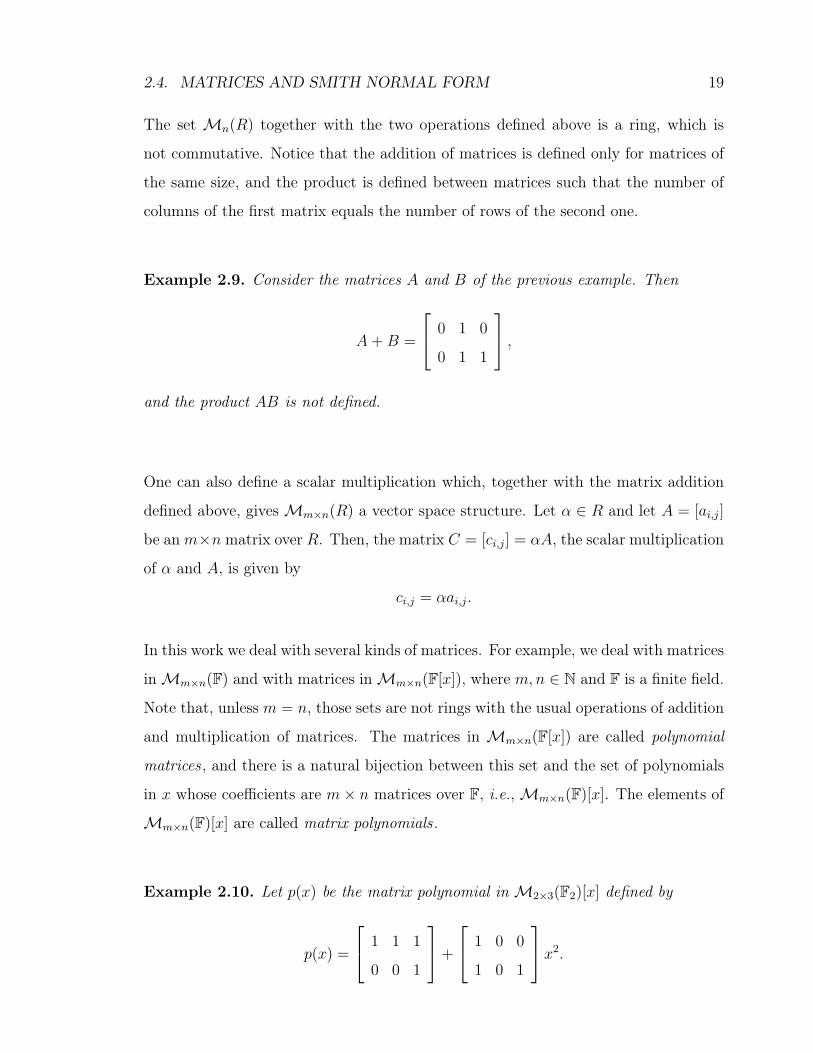
The set Mn(R) together with the two operations defined above is a ring, which is

not commutative. Notice that the addition of matrices is defined only for matrices of

the same size, and the product is defined between matrices such that the number of

columns of the first matrix equals the number of rows of the second one.

Example 2.9. Consider the matrices A and B of the previous example. Then

A+B =

2

4

0 1 0

0 1 1

3

5 ,

and the product AB is not defined.

One can also define a scalar multiplication which, together with the matrix addition

defined above, gives Mm⇥n(R) a vector space structure. Let ↵ 2 R and let A = [ai,j]

be an m⇥n matrix over R. Then, the matrix C = [ci,j] = ↵A, the scalar multiplication

of ↵ and A, is given by

ci,j = ↵ai,j.

In this work we deal with several kinds of matrices. For example, we deal with matrices

in Mm⇥n(F) and with matrices in Mm⇥n(F[x]), where m,n 2 N and F is a finite field.

Note that, unless m = n, those sets are not rings with the usual operations of addition

and multiplication of matrices. The matrices in Mm⇥n(F[x]) are called polynomial

matrices , and there is a natural bijection between this set and the set of polynomials

in x whose coefficients are m⇥ n matrices over F, i.e., Mm⇥n(F)[x]. The elements of

Mm⇥n(F)[x] are called matrix polynomials .

Example 2.10. Let p(x) be the matrix polynomial in M2⇥3(F2)[x] defined by

p(x) =

2

4

1 1 1

0 0 1

3

5

+

2

4

1 0 0

1 0 1

3

5 x2.


Then, the corresponding polynomial matrix in M2⇥3(F2[x]) is

P =

2

4

1 + x21 1

x20 1 + x2

3

5 .

If A is an m ⇥ n matrix, then the transpose matrix of A is denoted by AT and is

the n⇥m matrix whose (i, j)th entry is the same as the (j, i)th entry of the original

matrix A.

Example 2.11. Let A and B be the following matrices over R:

A =

2

6

6

6

4

1

2

3

3

7

7

7

5

and B =

2

4

1 2 3

4 5 6

3

5 .

Then,

AT=

h

1 2 3

i

and BT=

2

6

6

6

4

1 4

2 5

3 6

3

7

7

7

5

.

For an m ⇥ n matrix A, the submatrix Ai,j is obtained by deleting the ith row and

the jth column of A.

Example 2.12. Consider the matrix B of the previous example. Then B1,2 = [4, 6].

With each n ⇥ n matrix A = [ai,j] there is associated a unique number called the

determinant of A and written det(A) or |A|. The determinant of A can be computed

recursively as follows:

1. |A| = a1,1, if n = 1;

2. |A| = a1,1a2,2 � a1,2a2,1, if n = 2;

3. |A| =Pn

j=1(�1)

1+ja1,j|A1,j|, if n > 2.


It is well known that an n⇥ n matrix A has rank n if and only if the determinant of

A is not zero [McC71].

For an n⇥ n matrix A, the adjoint matrix of A is the matrix

adj(A) = [ci,j],

where

ci,j = (�1)

i+jdet(Aj,i).

Example 2.13. Consider the matrices

A =

2

6

6

6

4

1 0 1

0 1 0

1 0 0

3

7

7

7

5

and B =

2

6

6

6

4

1 1 0

0 0 1

0 0 0

3

7

7

7

5

,

defined over F2. Then, det(A) = 1, det(B) = 0,

adj(A) =

2

6

6

6

4

0 0 1

0 1 0

1 0 1

3

7

7

7

5

, and adj(B) =

2

6

6

6

4

0 0 1

0 0 1

0 0 0

3

7

7

7

5

.

Let A to be an n⇥ n matrix. A is called invertible (also non-singular) if there exists

an n⇥ n matrix B such that

AB = BA = In.

If this is the case, the matrix B is uniquely determined by A and is called the inverse

of A, denoted by A�1. The inverse of A can be computed in several ways. For example,

A�1=

1

det(A)adj(A).

Furthermore, A is invertible if and only if det(A) 6= 0 or, equivalently, rank(A) = n

[McC71]. The set of all n⇥n invertible matrices over R is denoted by GLn(R), which

stands for general linear group of degree n over R.


Example 2.14. The matrix B of the previous example is not invertible, while the

matrix A is invertible and A�1= adj(A).

Proposition 2.15 ([MP13]). Let Fq be a finite field with q 2 N elements and n 2 N.

Then

|GLn(Fq)| =n�1Y

i=0

(qn � qi).

Notice that non-square matrices are not invertible. However, they can be left or right

invertible. An m⇥ n matrix A is left (right) invertible if there is an n⇥m matrix B

such that BA = In (AB = Im). Such a matrix B is called a left (right) inverse of A.

One knows that A is left (right) invertible if and only if rank(A) = n (rank(A) = m),

i.e., the columns (rows) of A are linearly independent. One says that a matrix is in

reduced row echelon form if and only if all the following conditions hold:

• the first non-zero entry in each row is 1;

• each row has its first non-zero entry in a later column than any previous rows;

• all entries above and below the first non-zero entry of each row are zero;

• all rows having nothing but zeros are below all other rows of the matrix.

The matrix is said to be in reduced column echelon form if its transpose matrix is in

reduced row echelon form.

Example 2.16. The following matrix over F2 is in reduced row echelon form but is

not in reduced column echelon form:

2

6

6

6

4

0 1 1 0 0

0 0 0 1 0

0 0 0 0 0

3

7

7

7

5

.

Let A and B be two matrices with the same number of rows. We define the augmented

matrix [A|B] as the matrix obtained by appending the columns of the matrices A and

B.


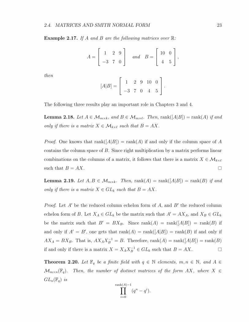
Example 2.17. If A and B are the following matrices over R:

A =

2

4

1 2 9

�3 7 0

3

5 and B =

2

4

10 0

4 5

3

5 ,

then

[A|B] =

2

4

1 2 9 10 0

�3 7 0 4 5

3

5 .

The following three results play an important role in Chapters 3 and 4.

Lemma 2.18. Let A 2 Mm⇥k, and B 2 Mm⇥`. Then, rank([A|B]) = rank(A) if and

only if there is a matrix X 2 Mk⇥` such that B = AX.

Proof. One knows that rank([A|B]) = rank(A) if and only if the column space of A

contains the column space of B. Since right multiplication by a matrix performs linear

combinations on the columns of a matrix, it follows that there is a matrix X 2 Mk⇥`

such that B = AX.

Lemma 2.19. Let A,B 2 Mm⇥k. Then, rank(A) = rank([A|B]) = rank(B) if and

only if there is a matrix X 2 GLk such that B = AX.

Proof. Let A0 be the reduced column echelon form of A, and B0 the reduced column

echelon form of B. Let XA 2 GLk be the matrix such that A0= AXA, and XB 2 GLk

be the matrix such that B0= BXB. Since rank(A) = rank([A|B]) = rank(B) if

and only if A0= B0, one gets that rank(A) = rank([A|B]) = rank(B) if and only if

AXA = BXB. That is, AXAX�1B = B. Therefore, rank(A) = rank([A|B]) = rank(B)

if and only if there is a matrix X = XAX�1B 2 GLk such that B = AX.

Theorem 2.20. Let Fq be a finite field with q 2 N elements, m,n 2 N, and A 2

Mm⇥n(Fq). Then, the number of distinct matrices of the form AX, where X 2

GLn(Fq) isrank(A)�1Y

i=0

(qn � qi).


Proof. Let A 2 Mm⇥n(Fq). We show that the number of matrices X 2 GLn(Fq)

such that AX = A isQn�1

i=rank(A)(qn � qi), when rank(A) 6= n, and equals 1 when

rank(A) = n. The result then follows from the well-known size of GLn(Fq) (given in

Proposition 2.15).

Let X 2 GLn(Fq) be such that AX = A. Then, there are n � rank(A) rows in X

whose entries can be arbitrarily chosen to have a solution of AX = A. But, since

X has to be invertible, one has qn � qrank(A) possibilities for the first of those rows,

qn � qrank(A)+1 for the second, qn � qrank(A)+2 for the third, and so on. Therefore, there

are (qn � qrank(A))(qn � qrank(A)+1

) · · · (qn � qn�1) matrices X that satisfy the required

condition.

Let V be a vector subspace of Fn with dimension k, where F is a field and n 2 N.

The unique basis {b1, b2, . . . , bk} of V such that the matrix [b1 b2 · · · bk] is in reduced

column echelon form will be here referred to as the standard basis of V .

Two m⇥ n matrices A,B, with entries in a PID, R, are said to be equivalent if there

exist matrices P 2 GLm(R) and N 2 GLn(R) such that B = PAN .

It is clear that matrix equivalence is an equivalence relation in the set Mm⇥n(R).

The following result is well known (see [Jac85] or [New72, Theorem II.9]).

Theorem 2.21. Let R be a principal ideal domain. Every matrix A 2 Mm⇥n(R) is

equivalent to a matrix of the form

D = diag(d1, d2, . . . , dr, 0, . . . , 0) =

2

6

6

6

6

6

6

6

6

6

6

6

6

6

4

d1. . . 0

dr

0

0 . . .

0

3

7

7

7

7

7

7

7

7

7

7

7

7

7

5

where r is the rank of A, di 6= 0 and di | di+1, i.e. di divides di+1, for 1 i r�1. The

matrix D is called the Smith normal form of A, denoted SNF(A), and the elements di

2.5. CAYLEY-HAMILTON THEOREM AND SOME IMPLICATIONS 25

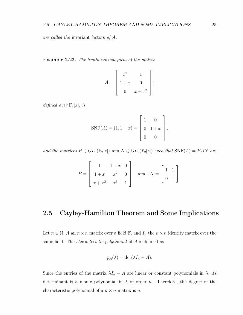
are called the invariant factors of A.

Example 2.22. The Smith normal form of the matrix

A =

2

6

6

6

4

x21

1 + x 0

0 x+ x2

3

7

7

7

5

,

defined over F2[x], is

SNF(A) = (1, 1 + x) =

2

6

6

6

4

1 0

0 1 + x

0 0

3

7

7

7

5

,

and the matrices P 2 GL3(F2[z]) and N 2 GL2(F2[z]) such that SNF(A) = PAN are

P =

2

6

6

6

4

1 1 + x 0

1 + x x20

x+ x2 x31

3

7

7

7

5

and N =

2

4

1 1

0 1

3

5 .

2.5 Cayley-Hamilton Theorem and Some Implications

Let n 2 N, A an n⇥n matrix over a field F, and In the n⇥n identity matrix over the

same field. The characteristic polynomial of A is defined as

pA(�) = det(�In � A).

Since the entries of the matrix �In � A are linear or constant polynomials in �, its

determinant is a monic polynomial in � of order n. Therefore, the degree of the

characteristic polynomial of a n⇥ n matrix is n.


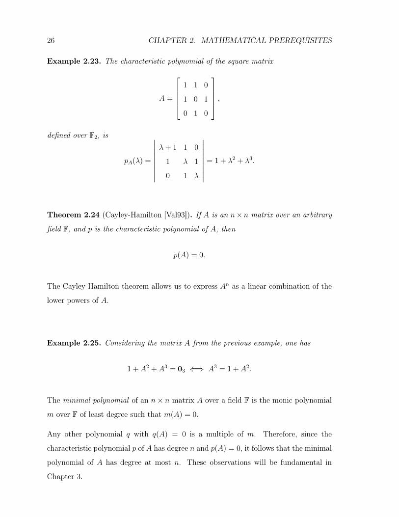
Example 2.23. The characteristic polynomial of the square matrix

A =

2

6

6

6

4

1 1 0

1 0 1

0 1 0

3

7

7

7

5

,

defined over F2, is

pA(�) =

�

�

�

�

�

�

�

�

�

�+ 1 1 0

1 � 1

0 1 �

�

�

�

�

�

�

�

�

�

= 1 + �2 + �3.

Theorem 2.24 (Cayley-Hamilton [Val93]). If A is an n⇥n matrix over an arbitrary

field F, and p is the characteristic polynomial of A, then

p(A) = 0.

The Cayley-Hamilton theorem allows us to express An as a linear combination of the

lower powers of A.

Example 2.25. Considering the matrix A from the previous example, one has

1 + A2+ A3

= 03 () A3= 1 + A2.

The minimal polynomial of an n⇥ n matrix A over a field F is the monic polynomial

m over F of least degree such that m(A) = 0.

Any other polynomial q with q(A) = 0 is a multiple of m. Therefore, since the

characteristic polynomial p of A has degree n and p(A) = 0, it follows that the minimal

polynomial of A has degree at most n. These observations will be fundamental in

Chapter 3.

2.6. LINEAR MAPS 27

2.6 Linear Maps

Let V and W be vector spaces over the same field F. A mapping f : V ! W is called

a linear transformation, linear map or an homomorphism of V into W , if the following

conditions are true:

• f(v1 + v2) = f(v1) + f(v2), for all v1, v2 in V ;

• f(↵v) = ↵f(v), for all ↵ in F and for all v in V .

The first condition states that addition is preserved under the mapping f . The second

asserts that also scalar multiplication is preserved under the mapping f . This is

equivalent to require that the same happens for any linear combination of vectors,

i.e., that for any vectors v1, . . . , vn 2 V , and scalars ↵1, . . . ,↵n 2 F, the following

equality holds:

f(↵1v1 + · · ·+ ↵nvn) = ↵1f(v1) + · · ·+ ↵nf(vn).

Denoting the zero elements of the vector spaces V and W by 0V and 0W respectively,

it follows that f(0V ) = 0W because letting ↵ = 0 in the second condition one gets:

f(0V ) = f(0 · 0V ) = 0f(0V ) = 0W .

An homomorphism which is a bijective mapping is called a linear isomorphism, and

if there exists an isomorphism ' of V onto W we say that V is isomorphic to W ,

denoted by V ' W , and ' is called a vector space isomorphism.

If V and W are finite dimensional vector spaces, and an ordered basis is defined for

each vector space, then every linear map from V to W can be represented by a matrix.

Moreover, matrices yield examples of linear maps. For example, if A is an m⇥n matrix

over a ring R, then A defines a linear map from Rn to Rm by sending the column vector

v 2 Rn to the column vector Av 2 Rm.


Now, let us see how to construct the matrix of a linear map. Let m,n 2 N be the

dimensions of the vector spaces V and W , respectively. Let f : V ! W be a linear

transformation and let BV = {v1, . . . , vm} be a basis for V . Then, every vector v in V

is uniquely determined by the coefficients ↵1, . . . ,↵m in F such that

v = ↵1v1 + · · ·+ ↵mvm.

Since f is a linear map, one has:

f(↵1v1 + · · ·+ ↵mvm) = ↵1f(v1) + · · ·+ ↵mf(vm),

which implies that the function f is entirely determined by the vectors f(v1), . . . , f(vm).

Now let BW = {w1, . . . , wn} be a basis for W . Then, we can represent each vector

f(vj), for j = 1, . . . ,m, as

f(vj) = a1,jw1 + · · ·+ am,jwm.

Thus the function f is entirely determined by the values of ai,j, for i = 1, . . . ,m and

j = 1, . . . , n. If we put these values into an m⇥n matrix M , then we can conveniently

use it to compute the vector output of f for any vector v in V . To obtain M , every

column j of M is a vector2

6

6

6

4

a1,j...

am,j

3

7

7

7

5

corresponding to f(vj) as defined above. In other words, every column j = 1, . . . , n

has a corresponding vector f(vj) whose coordinates a1j, . . . , am,j are the elements of

that column. The matrix constructed in this way is called the matrix of the linear

application relative to the bases BV and BW . Left multiplication by A takes a vector

written in terms of BV , applies f , and writes the result in terms of BW . It is then

obvious that a linear map may be defined by many matrices, since the values of the

elements of a matrix depend on the bases chosen.

2.6. LINEAR MAPS 29

Below we present an example where we compute the matrix of a linear application

relative to the standard bases of the vector spaces considered. This is the simplest

case, but is also the most relevant for this work.

Example 2.26. Let f : F32 ! F2

2 be the mapping defined by:

f(x, y, z) = (x+ y, z).

First, let us see that f is linear.

1. Let v = (v1, v2, v3), w = (w1, w2, w3) 2 F32. Then

f(v + w) = f(v1 + w1, v2 + w2, v3 + w3)

= (v1 + w1 + v2 + w2, v3 + w3)

= (v1 + v2, v3) + (w1 + w2, w3)

= f(v) + f(w).

2. Let ↵ 2 F2 and v = (v1, v2, v3) 2 F32. Then

f(↵v) = f(↵v1,↵v2,↵v3)

= (↵v1 + ↵v2,↵v3)

= ↵(v1 + v2, v3)

= ↵f(v).

Since addition and scalar multiplication are preserved under f , one concludes that f

is a linear map.

Now, let B be the standard basis of F32, i.e.,

B = {(1, 0, 0); (0, 1, 0); (0, 0, 1)}.


One has,

f(1, 0, 0) = (1, 0)

f(0, 1, 0) = (1, 0)

f(0, 0, 1) = (0, 1).

Therefore, the matrix of f relative to B and the standard basis of F22 is

2

4

1 1 0

0 0 1

3

5 ,

and, for example,

f(1, 1, 0) =

2

4

1 1 0

0 0 1

3

5

2

6

6

6

4

1

1

0

3

7

7

7

5

=

2

4

0

0

3

5 .

Given a matrix, A, of a linear application, f , it is well known that if the rows (columns)

of A are linearly independent, then f is surjective (injective).

Example 2.27. The mapping f defined in the previous example is surjective, because

the matrix of the application has linearly independent rows.

Chapter 3

Linear Finite Transducers

3.1 Preliminaries on Finite Transducers

In what follows, an alphabet is a non-empty finite set of elements. The elements of

an alphabet are called symbols or letters . Given an alphabet A, a finite sequence of

symbols from A, say a0a1 · · · a`�1, is called a word over A, and ` its length. When

` = 0, the sequence a0a1 · · · a`�1 is an empty sequence which contains no element

and it is called the empty word . We use " to denote the empty word, and |↵| to

denote the length of the word ↵. We let An be the set of words of length n, where

n 2 N0, and A0= {"}. We put A?

= [n�0An, the set of all finite words, and

A!= {a0a1 · · · an · · · | ai 2 A} is the set of infinite words.

Let ↵ = a0a1 · · · am�1 and � = b0b1 · · · bn�1 be two words in A? of length m and n,

respectively. The concatenation of ↵ and � is a0a1 · · · am�1b0b1 · · · bn�1, which is also

a word in A?, of length m+n, and is denoted by ↵�. Clearly, ↵" = "↵ = ↵. Similarly,

if ↵ = a0a1 · · · am�1 2 A? and � = b0b1 · · · bn�1 · · · 2 A!, then the concatenation of ↵

and � is the element a0a1 · · · am�1b0b1 · · · bn�1 · · · of A!. It is obvious that "� = �.

For any U, V ✓ A?, the concatenation of U and V is the set {↵� | ↵ 2 U, � 2 V }.

In the context of this work, a finite transducer (FT) is a deterministic finite state

31

32 CHAPTER 3. LINEAR FINITE TRANSDUCERS

sequential machine which, in any given state, reads a symbol from a set X , produces

a symbol from a set Y , and switches to another state. Thus, given an initial state and

a finite input sequence, a transducer produces an output sequence of the same length.

The formal definition of a finite transducer is the following.

Definition 3.1. A finite transducer is a quintuple hX ,Y , S, �,�i, where:

• X is a non-empty finite set, called the input alphabet;

• Y is a non-empty finite set, called the output alphabet;

• S is a non-empty finite set called the set of states;

• � : S ⇥ X ! S, called the state transition function;

• � : S ⇥ X ! Y, called the output function.

These transducers are deterministic and can be seen as having all the states as final.

Every state in S can be used as initial, and this gives rise to a determinist transducer

in the usual sense, also known as Mealy machine [Sta72, Rut06]. Therefore, in what

follows, a transducer is a family of classical transducers that share the same underlying

digraph.

Let M = hX ,Y , S, �,�i be a finite transducer. The state transition function � and the

output function � can be extended to finite words, i.e., elements of X ?, recursively, as

follows:

�(s, ") = s, �(s, x↵) = �(�(s, x),↵),

�(s, ") = ", �(s, x↵) = �(s, x) �(�(s, x),↵),

where s 2 S, x 2 X , and ↵ 2 X ?. In an analogous way, � may be extended to X !.

From these definitions it follows that one has, for all s 2 S,↵, � 2 X ?,

�(s,↵�) = �(�(s,↵), �)

3.1. PRELIMINARIES ON FINITE TRANSDUCERS 33

and, for all s 2 S,↵ 2 X ?, � 2 X ? [ X !,

�(s,↵�) = �(s,↵) �(�(s,↵), �).

Example 3.2. Let M = h{0, 1}, {a, b}, {s1, s2}, �,�i be the transducer defined by:

�(s1, 0) = s1, �(s1, 1) = s2, �(s2, 0) = s1, �(s2, 1) = s2,

�(s1, 0) = a, �(s1, 1) = a, �(s2, 0) = b, �(s2, 1) = b.

Then, for example,

�(s1, 01) = �(�(s1, 0), 1) = �(s1, 1) = s2,

�(s1, 01) = �(s1, 0)�(�(s1, 0), 1) = a�(s1, 1) = aa,

and

�(s1, 0010110) = s1,

�(s1, 0010110) = aaababb.

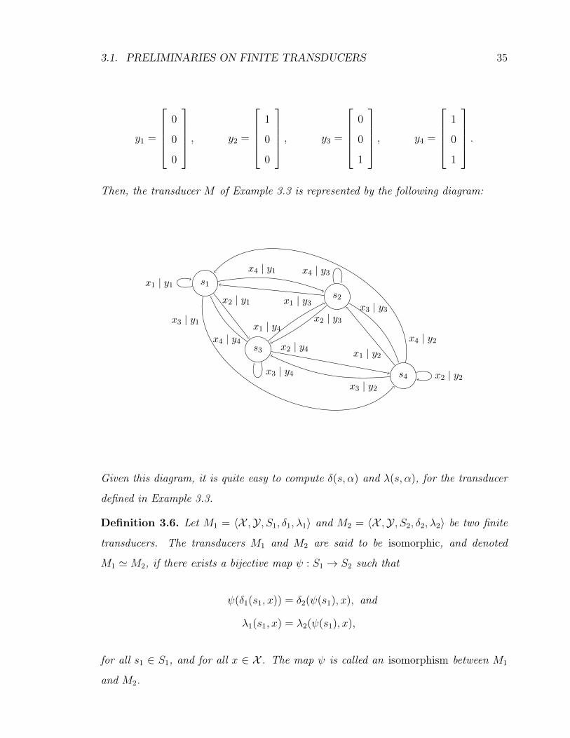
Example 3.3. Let M = hF22,F3

2,F22, �,�i be the transducer defined by:

�(s, x) = As+Bx,

�(s, x) = Cs+Dx,

for all s 2 F22, x 2 F2

2, and where

A =

2

4

0 1

0 0

3

5 , B =

2

4

0 1

1 1

3

5 , C =

2

6

6

6

4

0 1

0 0

1 1

3

7

7

7

5

, and D =

2

6

6

6

4

0 0

0 0

0 0

3

7

7

7

5

.


Take s =

2

4

1

0

3

5 and ↵ =

2

4

1

1

3

5

2

4

1

0

3

5

2

4

0

0

3

5

2

4

1

0

3

5

2

4

1

1

3

5. Then,

� (s,↵) =

2

4

0

0

3

5 ,

� (s,↵) =

2

6

6

6

4

0

0

1

3

7

7

7

5

2

6

6

6

4

0

0

1

3

7

7

7

5

2

6

6

6

4

1

0

1

3

7

7

7

5

2

6

6

6

4

0

0

1

3

7

7

7

5

2

6

6

6

4

1

0

1

3

7

7

7

5

.

M is what is called a linear finite transducer. The formal definition will be given in

Section 3.2.

A transducer can be represented by a diagram that is a digraph with labeled nodes

and arcs, where loops and multiple arcs are allowed. Each state of the transducer is

represented by a node, and each arc indicates a transition between states. The label

of each arc is a compound symbol of the form i | o, where i and o stand for the input

and output symbol, respectively. This representation is useful to deal by hand with

the computations of some examples presented in this chapter.

Example 3.4. The transducer M defined in Example 3.2 is represented by the diagram

below.

s1 s2

1 | a

0 | b

0 | a 1 | b

Example 3.5. Let

x1 =

2

4

0

0

3

5 , x2 =

2

4

1

0

3

5 , x3 =

2

4

0

1

3

5 , x4 =

2

4

1

1

3

5 ,

s1 =

2

4

0

0

3

5 , s2 =

2

4

1

0

3

5 , s3 =

2

4

0

1

3

5 , s4 =

2

4

1

1

3

5


y1 =

2

6

6

6

4

0

0

0

3

7

7

7

5

, y2 =

2

6

6

6

4

1

0

0

3

7

7

7

5

, y3 =

2

6

6

6

4

0

0

1

3

7

7

7

5

, y4 =

2

6

6

6

4

1

0

1

3

7

7

7

5

.

Then, the transducer M of Example 3.3 is represented by the following diagram:

s1s2

s3

s4

x1 | y1x4 | y1

x2 | y1

x3 | y1

x4 | y3

x1 | y3x2 | y3

x3 | y3

x3 | y4

x4 | y4x1 | y4

x2 | y4

x2 | y2

x4 | y2x1 | y2

x3 | y2

Given this diagram, it is quite easy to compute �(s,↵) and �(s,↵), for the transducer

defined in Example 3.3.

Definition 3.6. Let M1 = hX ,Y , S1, �1,�1i and M2 = hX ,Y , S2, �2,�2i be two finite

transducers. The transducers M1 and M2 are said to be isomorphic, and denoted

M1 ' M2, if there exists a bijective map : S1 ! S2 such that

(�1(s1, x)) = �2( (s1), x), and

�1(s1, x) = �2( (s1), x),

for all s1 2 S1, and for all x 2 X . The map is called an isomorphism between M1

and M2.


Remark 3.7. Let M = hX ,Y , S, �,�i be a finite transducer, S 0 a non-empty set, and

: S ! S 0 a bijective map. The transducer M = hX ,Y , S 0, � ,� i defined by

� (s0, x) =

�

��

�1(s0), x

��

,

� (s0, x) = �

�

�1(s0), x

�

,

for all s0 2 S 0, x 2 X , is isomorphic to M because satisfies the two conditions in

the previous definition:

� ( (s), x) = �

�( �1( (s)), x)

�

= (�(s, x));

� ( (s), x) = �( �1( (s)), x) = �(s, x).

Definition 3.8. Let M1 = hX ,Y1, S1, �1,�1i and M2 = hX ,Y2, S2, �2,�2i be two finite

transducers. Let s1 2 S1, and s2 2 S2. One says that s1 and s2 are equivalent, and

denote this relation by s1 ⇠ s2, if

8↵ 2 X ?, �1(s1,↵) = �2(s2,↵).

It is obvious that if s1 ⇠ s2, then

8x 2 X , �1(s1, x) ⇠ �2(s2, x).

Let M = hX ,Y , S, �,�i be a finite transducer. Trivially, the relation ⇠ is an equiva-

lence relation on S. As usual, we will denote by [s]⇠ or [s] the equivalence class that

contains s, and by S/⇠ the set of equivalence classes of S, i.e., S/⇠ = {[s]⇠ | s 2 S}.

Example 3.9. Let M = hF2,F2, {s1, s2, s3}, �,�i be the transducer induced by the

diagram:


s1 s2

s3

0 | 1

0 | 11 | 1

1 | 10 | 0

1 | 0

and let M 0= hF2,F2, {s01, s02}, �0,�0i be the transducer induced by:

s01 s020 | 1

1 | 10 | 0

1 | 0

Then

• s2 ⇠ s02, because 8↵ 2 X ?, �(s2,↵) = 0 · · · 0 = �0(s02,↵);

• s1 ⇠ s3 ⇠ s01.

To prove that s1 ⇠ s3, let ↵ be a non-empty word in F?2. Then, either ↵ is of the form

0� or ↵ is of the form 1�, for some � in F?2. In the first case, one has

�(s1, 0�) = �(s1, 0)�(�(s1, 0), �) = 1�(s2, �),

and

�(s3, 0�) = �(s3, 0)�(�(s3, 0), �) = 1�(s2, �).

It follows that �(s1, 0�) = �(s3, 0�), for all � 2 X ?. Analogously,

�(s1, 1�) = 1�(s1, �) = �(s3, 1�),

for all � 2 X ?. Therefore, 8↵ 2 X ?, �(s1,↵) = �(s3,↵), i.e., s1 ⇠ s3. It is also easy

to see that s1 ⇠ s01.




�(s, x) = As+Bx,

�(s, x) = Cs+Dx,

for all s 2 F22, x 2 F2

2, and where

A =

2

4

1 0

1 0

3

5 , B =

2

4

1 1

0 1

3

5 , C =

2

4

0 0

1 1

3

5 , and D =

2

4

1 0

1 1

3

5 .

The pair of states

2

4

1

0

3

5 and

2

4

0

1

3

5 are equivalent, as well as

2

4

0

0

3

5 and

2

4

1

1

3

5.

In Section 3.3 we present a method to directly check the equivalence of states for linear

finite transducers. We now introduce the notion of equivalent transducers used in this

context.

Definition 3.11. Let M1 = hX ,Y1, S1, �1,�1i and M2 = hX ,Y2, S2, �2,�2i be two FTs.

M1 and M2 are said to be equivalent, and denote this by M1 ⇠ M2, if the following

two conditions are simultaneously satisfied:

• 8s1 2 S1, 9s2 2 S2 : s1 ⇠ s2;

• 8s2 2 S2, 9s1 2 S1 : s1 ⇠ s2.

The relation ⇠ defines an equivalence relation on the set of finite transducers.

Example 3.12. The transducers M and M 0 of Example 3.9 are equivalent, since

s1 ⇠ s3 ⇠ s01 and s2 ⇠ s02.

Definition 3.13. Let M = hX ,Y , S, �,�i be a finite transducer. Considering the

equivalence relation ⇠ on the set of states, one defines the quotient transducer M/⇠ =

hX ,Y , S/⇠, �⇠,�⇠i in the following way

�⇠([s], x) = [�(s, x)] and �⇠([s], x) = �(s, x),


for all [s] 2 S/⇠, x 2 X .

Lemma 3.14. �⇠ and �⇠ are well defined.

Proof. Let [s1], [s2] 2 S/⇠ such that [s1] = [s2]. Since [s1] = [s2] if and only if s1 ⇠ s2,

it follows that

�(s1, x) ⇠ �(s2, x), 8x 2 X , and �(s1,↵) = �(s2,↵), 8↵ 2 X ?.

Consequently,

[�(s1, x)] = [�(s2, x)], 8x 2 X , and �(s1,↵) = �(s2,↵), 8↵ 2 X ?.

Thus, �⇠ and �⇠ are well defined.

Lemma 3.15. For all s 2 S, ↵ 2 X ?, one has

�⇠([s],↵) = [�(s,↵)].

Proof. (by induction on the length of ↵)

The case |↵| = 1 is immediate from definition of �⇠. Assume that, given n 2 N, the

equality holds when |↵| = n. Let x 2 X . Then

�⇠([s],↵x) = �⇠(�⇠([s],↵), x),

= �⇠([�(s,↵)], x), from hypothesis,

= [�(�(s,↵), x)], from the definition of �⇠,

= [�(s,↵x)].

Lemma 3.16. For all s 2 S, one has s ⇠ [s], i.e.,

8↵ 2 X ?, �(s,↵) = �⇠([s],↵).


Proof. (by induction on the length of ↵)

The case |↵| = 1 is obvious from definition of �⇠. Assume that, given n 2 N, the

equality holds when |↵| = n. Let x 2 X . Then

�⇠([s],↵x) = �⇠(�⇠([s],↵), x),

= �(s,↵)�⇠([�(s,↵)], x), from hypothesis,

= �(s,↵)�(�(s,↵), x), from the definition of �⇠,

= �(s,↵x).

Theorem 3.17. Let M = hX ,Y , S, �,�i be a finite transducer. Then, the quotient

transducer M/⇠ = hX ,Y , S/⇠, �⇠,�⇠i is equivalent to M .

Proof. To prove that M/⇠ is equivalent to M , by definition, one needs to prove that:

1. 8s 2 S, 9s0 2 S/⇠ : s ⇠ s0;

2. 8s0 2 S/⇠, 9s 2 S : s ⇠ s0.

To prove the first condition, one just needs to take s0 = [s], because, by Lemma 3.16,

s ⇠ [s]. To prove the second condition, let s0 2 S/⇠. Take s 2 S such that s0 = [s].

Since, s ⇠ [s], the condition follows.

Definition 3.18. A finite transducer is called minimal if it has no equivalent trans-

ducer with fewer states.

Proposition 3.19. A finite transducer is minimal if and only if it has no pair of

equivalent states.

Proof. Let M = hX ,Y , S, �,�i be a finite transducer. We prove the “if part” by proving

that if M is not minimal, then M has at least a pair of equivalent states. Assume that


M is not minimal. Then, by definition, there is a transducer M 0= hX ,Y 0, S 0, �0,�0i

such that M ⇠ M 0 and |S 0| < |S|. From M ⇠ M 0, it follows that

8s 2 S, 9s0 2 S 0, s ⇠ s0.

Since |S 0| < |S|, this implies that there are at least two states s1, s2 2 S such that

s1 ⇠ s0 ⇠ s2, for some s0 2 S 0. Thus, M has at least a pair of equivalent states.

To prove the “only if” part, we prove that if M has at least a pair of equivalent states,

then M is not minimal. Let M = hX ,Y , S, �,�i be a finite transducer which has at

least a pair of equivalent states. Then |S/⇠| |S|�1. Consequently, M is not minimal

because M/⇠ is an equivalent transducer (by Theorem 3.17) with fewer states.

Example 3.20. The transducer M defined in Example 3.10 is equivalent to the trans-

ducer M 0= hF2

2,F22,F2, �

0,�0i defined by:

�0(s0, x) = A0s0 +B0x,

�0(s0, x) = C 0s0 +D0x,

for all s0 2 F22, x 2 F2

2, and where

A0=

h

0

i

, B0=

h

1 0

i

, C 0=

2

4

0

1

3

5 , and D0=

2

4

1 0

1 1

3

5 .

First notice that M 0 has only two states, s01 = 0 and s02 = 1, which are not equivalent

since, for example,

�0

0

@s01,

2

4

1

0

3

5

1

A

=

2

4

1

1

3

5 6=

2

4

1

0

3

5

= �0

0

@s02,

2

4

1

0

3

5

1

A .

Therefore M 0 is minimal. It can also be shown that s01 ⇠ s1 ⇠ s2 and s01 ⇠ s3 ⇠ s4,

where s1 =

2

4

1

0

3

5, s2 =

2

4

0

1

3

5, s3 =

2

4

0

0

3

5, and s4 =

2

4

1

1

3

5.


Example 3.21. The transducer M of Example 3.9 is not minimal because states s1

and s3 are equivalent. The transducer M 0, in the same example, is minimal because

s01 and s02 are not equivalent (for example, �0(s01, 0) = 1 6= 0 = �0(s02, 0)).

Theorem 3.22. Let M = hX ,Y , S, �,�i be a finite transducer. The transducer M/⇠

is minimal.

Proof. Since M/⇠ is constructed in a way that all states equivalent to a given state

in M are collapsed into a single state of S/⇠, one concludes that M/⇠ has no pair of

equivalent states, i.e., M/⇠ is minimal.

From the previous theorem, constructing the quotient transducer of a finite transducer

M is a method to obtain a minimal FT equivalent to M . In Section 3.4, we adapt this

method to minimize linear finite transducers.

Example 3.23. Consider the transducer M of Example 3.9. One knows that s1 ⇠ s3.

Then, M/⇠ is the transducer induced by the diagram below.

[s1] [s2]0 | 1

1 | 10 | 0

1 | 0

The transducer M/⇠ is minimal and isomorphic to the transducer M 0 also presented in

Example 3.9 (it is quite obvious that the application : {[s1], [s2]} ! {s01, s02} defined

by ([s1]) = s01 and ([s2]) = s02 is an isomorphism between M/⇠ and M 0).

It is clear that if M1 ' M2, then M1 ⇠ M2. Conversely, if M1 and M2 are minimal

and equivalent, and Y1 = Y2, then it can be proven that M1 and M2 are isomorphic.

Just consider to be the relation ⇠ from S1 to S2 [Tao09, page 11]. Thus, a minimal

transducer is unique up to isomorphism.


3.1.1 Concepts on Invertibility

A fundamental concept in this work is the concept of injectivity that is behind the

invertibility property of the transducers used for cryptographic purposes. In fact, we

will talk about two concepts: the concept of !-injectivity and the concept of injectivity

with a certain delay. These two notions of injectivity were introduced, as far as we

know, by Tao, who called them weakly invertible and weakly invertible with a certain

delay , respectively [Tao09]. Here we use names that are more naturally related to how

these terms are used in other mathematical settings.

Definition 3.24. A finite transducer M = hX ,Y , S, �,�i is !-injective, if

8s 2 S, 8↵,↵0 2 X !, �(s,↵) = �(s,↵0) ) ↵ = ↵0.

That is, for any s 2 S, and any ↵ 2 X !, ↵ can be uniquely determined by s and

�(s,↵).

Definition 3.25. A finite transducer M = hX ,Y , S, �,�i is injective with delay ⌧ , or

⌧ -injective, with ⌧ 2 N0, if

8s 2 S, 8x, x0 2 X , 8↵,↵0 2 X ⌧ , �(s, x↵) = �(s, x0↵0) ) x = x0.

That is, for any s 2 S, x 2 X , and ↵ 2 X ⌧ , x is uniquely determined by s and

�(s, x↵).

To simplify, an equivalence class formed by !-injective FTs is said to be !-injective.

Analogously, an equivalence class of ⌧ -injective FTs, for some ⌧ 2 N0, is said to be

⌧ -injective.

Later in this work, we deal with the case X = F`, where F is a field, and it will be useful

to identify the elements of X ! with the elements of F[[z]]`, by replacing x0x1x2 · · · withP

i�0 xizi. In that context, and from the definition of congruence modulo n relation,


a finite transducer M = hX ,Y , S, �,�i is injective with delay ⌧ if and only if

�(s,X) ⌘ �(s,X 0) (mod z⌧+1

) ) X ⌘ X 0(mod z), (3.1)

for all s 2 S, and X,X 0 2 F[[z]]`.

Example 3.26. The transducer presented in Example 3.2, and which is represented

by the diagram

s1 s2

1 | a

0 | b

0 | a 1 | b

is injective with delay 1. To prove that, one has to compute the output for every state

and every input sequence of length 2:

�(s1, 00) = aa, �(s2, 00) = ba, �(s1, 10) = ab, �(s2, 10) = bb,

�(s1, 01) = aa, �(s2, 01) = ba, �(s1, 11) = ab, �(s2, 11) = bb.

From these outputs, one can conclude that

8 s 2 {s1, s2}, 8 x0 x1, x00 x

01 2 {0, 1}2, �(s, x0x1) = �(s, x0

0x01) ) x0 = x0

0,

which proves, by definition, that the transducer is injective with delay 1. Moreover,

the transducer is not injective with delay 0 (for example, �(s1, 0) = a = �(s1, 1) and

0 6= 1).

Example 3.27. It can be proven that the transducer M of Example 3.3 is also injective

with delay 1, and is not injective with delay 0.

In Chapter 5 we will see an efficient method for checking if a linear finite transducer

is injective with delay ⌧ , for any ⌧ 2 N0.


Example 3.28. The transducer M = h{0, 1}, {a, b}, {s1, s2}, �,�i induced by the dia-

gram

s1 s2

1 | a

0 | b

0 | a 1 | a

is not injective with delay 1 since, for example, �(s1, 01) = �(s1, 11) and 0 6= 1.

It is obvious that, if a finite transducer M is injective with some delay ⌧ 2 N0, then M

is also injective with delay k, for k � ⌧ , which implies that it is also !-injective. Tao

[Tao09, Corollary 1.4.3] proved the following result, which shows that the converse is

also true.

Theorem 3.29. Let M = hX ,Y , S, �,�i be a finite transducer. If M is !-injective,

then there exists a non-negative integer ⌧ |S|(|S|�1)2 such that M is injective with

delay ⌧ .

Example 3.30. From the previous theorem we may conclude that the transducer M

defined in Example 3.28 is not !-injective, since it is not injective with delay 1 and

the set of states has size 2.

Since every !-injective finite transducer is injective with some delay ⌧ , our study of

injectivity, presented in the following chapters, is confined to these latter transducers.

Naturally, injective transducers should have inverses of some sort. In order to describe

the appropriate concept we introduce a notion of an inverse state of a given state.

Definition 3.31. Let M = hX ,Y , S, �,�i and M 0= hY ,X , S 0, �0,�0i be two finite

transducers. Let s 2 S and s0 2 S 0. We say that s0 inverts s with delay ⌧ or s0 is an

inverse state with delay ⌧ of s when

8↵ 2 X !, �0 (s0,�(s,↵)) = �↵, for some � 2 X ⌧ .


The figure below gives a schematic representation of this concept with x1x2 · · · = ↵

and y1y2 · · · = �(s,↵).

s

M

s0

M 0

x1x2 · · · y1y2 · · · � x1x2 · · ·

Remark 3.32. In the previous definition one may replace X ! by X ?, but then one

should also replace �0(s0,�(s,↵)) = �↵ by �0(s0,�(s,↵)) = �↵0, where ↵0 consists of the

first |↵|� ⌧ characters of ↵.

Example 3.33. Let M 0= h{a, b}, {0, 1}, {s0}, �0,�0i be the finite transducer induced

by the following diagram:

s0a | 0 b | 1

We will see that the state s0 of M 0 inverts the states s1 and s2 of M with delay 1,

where M is the transducer defined in Example 3.2.

To prove that, it is enough to show that for all x1x2 2 {0, 1}2, and for all s 2 {s1, s2},

one has

�0(s0,�(s, x1x2)) = xx1, for some x 2 {0, 1}, (3.2)

because this implies that for all ↵ 2 {0, 1}!, and for all s 2 {s1, s2},

�0(s0,�(s,↵)) = x↵, for some x 2 {0, 1}.

Using the diagrams of the transducers one easily gets

�0(s0,�(s1, 00)) = �0(s0, aa) = 00, �0(s0,�(s1, 10)) = �0(s0, ab) = 01,

�0(s0,�(s1, 01)) = �0(s0, aa) = 00, �0(s0,�(s1, 11)) = �0(s0, ab) = 01,

�0(s0,�(s2, 00)) = �0(s0, ba) = 10, �0(s0,�(s2, 10)) = �0(s0, bb) = 11,


�0(s0,�(s2, 01)) = �0(s0, ba) = 10, �0(s0,�(s2, 11)) = �0(s0, bb) = 11.

This proves that (3.2) holds.

Definition 3.34. Let M = hX ,Y , S, �,�i be a finite transducer. One says that M is

left invertible with delay ⌧ if there is a transducer M 0= hY ,X , S 0, �0,�0i such that

8 s 2 S, 9 s0 2 S 0, s0 inverts s with delay ⌧.

The transducer M 0 is called a left inverse with delay ⌧ of M .

It is clear that, in the previous example, the transducer M 0 is a left inverse with delay

1 of M .

If M 0 is a left inverse with delay ⌧ of M , then M 0 can recover the input of M with a

delay of ⌧ input symbols.

The following result establishes the fundamental relation between the injectivity of a

transducer and the existence of a left inverse.

Theorem 3.35. A finite transducer M = hX ,Y , S, �,�i is injective with delay ⌧ if

and only if there exists a finite transducer M 0= hY ,X , S 0, �0,�0i such that M 0 is a left

inverse with delay ⌧ of M .

Proof. The necessary condition is proven by Tao [Tao09, Theorem 1.4.4]. To prove

the sufficient condition, assume that there is a transducer M 0 which is a left inverse

with delay ⌧ of M , for ⌧ 2 N0. Let s 2 S, x, x0 2 X , and ↵,↵0 2 X ⌧ . Then there is a

state s0 2 S 0 such that

�(s, x↵) = �(s, x0↵0) =) �0(s0,�(s, x↵)) = �0(s0,�(s, x0↵0

)) =) x = x0.

Therefore, M is injective with delay ⌧ .


3.1.2 Finite Transducers with Memory

Let A be a non-empty set and j 2 N. Define �j : Aj ⇥ A ! Aj by:

�j((a1, . . . , aj), a) = (a2, . . . , aj, a).

Definition 3.36. Let � : X h+1 ⇥ Yk �! Y, with h, k 2 N0 not simultaneously null,

and X ,Y two non-empty finite sets. Let M� =

⌦

X ,Y ,X h ⇥ Yk, ��,��↵

be the finite

transducer such that, for all x 2 X , ↵ 2 X h, � 2 Yk, and the state transition and

output functions are given by:

��(< ↵, � >, x) =< �h(↵, x), �k(�, y) >,

��(< ↵, � >, x) = y,

where y = �(↵, x, �) and < . . . > is used to denote the states of this transducer. M�

is called the finite transducer with memory (h, k) defined by �. If k = 0, then M� is

said to be a finite transducer with input memory (h, 0).

As the name suggests, a finite transducer with memory is completely defined by its

memory (h, k) and by the function �. Notice that �� and �� are explicitly given by

�. Below, there is a schematic representation of the state transition function for this

kind of transducers, where x1, . . . , xh, x 2 X and y1, . . . , yk, y 2 Y .

< x1, x2, . . . , xh, y1, y2, . . . , yk > < x2, . . . , xh, x, y2, . . . , yk, y >x | y

Example 3.37. Let M� be the finite transducer with memory of order (2, 1) defined

by the map � : F42 ! F2 with �(a, b, c, d) = c + b d. Then M� = hF2,F2,F3

2, ��,��i is

such that

��(< x1, x2, y1 >, x) = �(x1, x2, x, y1), and

��(< x1, x2, y1 >, x) =< x2, x,��(< x1, x2, y1 >, x) > .


Take s =< 1, 1, 1 > 2 F32. Then,

��(s, 0) = �(1, 1, 0, 1) = 1, and

��(s, 0) =< 1, 0, 1 > .

Usually, finite transducers with memory of order (h, k) are defined by the set of

equations

yt = �(xt�h, . . . , xt�1, xt, yt�k, . . . , yt�1), for t � 0,

starting with some initial state to which one assigns negative indices. For example,

the transducer in the previous example could be defined as follows. Let M� =

hF2,F2,F32, ��,��i be the finite transducer with memory of order (2, 1) defined by

yt = xt + xt�1 yt�1, for t � 0,

where s =< x�2, x�1, y�1 > is the initial state of the transducer. With this kind of

notation we are assuming that

y0y1 · · · = ��(< x�2, x�1, y�1 >, x0x1 · · · ).

where xi 2 F2, for i � �2, and yj 2 F2, for j � �1.


2, (F22)

2 ⇥ F32, �,�i be the finite transducer with memory

of order (2, 1) defined by

yt =

2

6

6

6

4

1 0

0 1

1 1

3

7

7

7

5

xt +

2

6

6

6

4

0 0

0 1

0 1

3

7

7

7

5

xt�2 + yt�1, for t � 0,

where xi 2 F22, for i � �2, yj 2 F3

2, for j � �1, and < x�2, x�1, y�1 > is the initial

state of the transducer.


Take x�2 =

2

4

1

0

3

5, x�1 =

2

4

0

1

3

5, y�1 =

2

6

6

6

4

1

0

1

3

7

7

7

5

, and s =< x�2, x�1, y�1 >. Then, for

example,

�

0

@s,

2

4

1

0

3

5

2

4

1

1

3

5

1

A

=

2

6

6

6

4

0

0

0

3

7

7

7

5

2

6

6

6

4

1

0

1

3

7

7

7

5

.

If, in the definition of finite transducer with memory, (Y ,+) is a group (not necessarily

Abelian) and the function � is of the form

� = f(x1, x2, . . . , xh, xh+1) + g(y1, y2, . . . , yk),

for some f : X h+1 ! Y and g : Yk ! Y , one says that M� is a separable finite trans-

ducer with memory, denoted by Mf,g. Notice that, in particular, a finite transducer

with input memory (h, 0) is a separable finite transducer.

Example 3.39. The transducer defined in the previous example is a separable finite

transducer, while the transducer defined in Example 3.37 is not separable.

The following result about separable finite transducers is mentioned by Zongduo et al.

[ZDL98] without proof.

Theorem 3.40. Let Y be a group, denoted additively. Then the separable transducer

Mf,g =⌦

X ,Y ,X h ⇥ Yk, �f,g,�f,g↵

is injective with delay ⌧ if and only if the transducer

Mf =

⌦

X ,Y ,X h, �f ,�f↵

is injective with delay ⌧ .

Proof. Notice that, given s1 2 X h, s2 2 Yk, x 2 X , one can write

�f,g(< s1, s2 >, x) = f(s1, x) + g(s2). (3.3)

Also, if s1 2 X h, s2 2 Yk, x 2 X , and ↵ 2 X ⌧ , then �f,g(< s1, s2 >, x↵) is just a

3.2. THE NOTION OF LINEAR FINITE TRANSDUCER 51

sequence of elements as in (3.3). Since, obviously,

f(s1, x) + g(s2) = f(s1, x0) + g(s2) () f(s1, x) = f(s1, x

0),

for all s1 2 X h, s2 2 Yk, x, x0 2 X , and ↵,↵0 2 X ⌧ , one concludes that

�f,g(< s1, s2 >, x↵) = �f,g(< s1, s2 >, x0↵0)

is equivalent to

�f (< s1 >, x↵) = �f (< s1 >, x0↵0).

From this, the claim made follows immediately.

3.2 The Notion of Linear Finite Transducer

Definition 3.41. If X ,Y and S are vector spaces over a field F, and both � : S⇥X ! S

and � : S ⇥ X ! Y are linear maps, then M = hX ,Y , S, �,�i is called a linear finite

transducer (LFT) over F, and we say that the size of M , denoted size(M), is the

dimension of S as a vector space.



�(s, x) = (s2 + x1, s1 + x2 + x3),

�(s, x) = (s1 + x1 + x3, s2 + x2),

for all s = (s1, s2) 2 F22, and for all x = (x1, x2, x3) 2 F3

2. The state transition function

� : F52 ! F2

2 and the output function � : F52 ! F2

2 are linear maps, therefore, M is

an LFT over F2 and the size of M is dim(F22) = 2. Moreover, if one considers the

standard bases of F52 and F2

2, those maps are represented in terms of matrices in the


following way

�(s, x) =

2

4

0 1 1 0 0

1 0 0 1 1

3

5

h

s1 s2 x1 x2 x3

iT

=

2

4

0 1

1 0

3

5

2

4

s1

s2

3

5

+

2

4

1 0 0

0 1 1

3

5

2

6

6

6

4

x1

x2

x3

3

7

7

7

5

=

2

4

0 1

1 0

3

5 s+

2

4

1 0 0

0 1 1

3

5 x,

�(s, x) =

2

4

1 0 1 0 1

0 1 0 1 0

3

5

h

s1 s2 x1 x2 x3

iT

=

2

4

1 0

0 1

3

5

2

4

s1

s2

3

5

+

2

4

1 0 1

0 1 0

3

5

2

6

6

6

4

x1

x2

x3

3

7

7

7

5

=

2

4

1 0

0 1

3

5 s+

2

4

1 0 1

0 1 0

3

5 x.

Let M = hX ,Y , S, �,�i be an LFT over a field F. If X ,Y , and S have dimensions

`, m and n, respectively, then there exist matrices A 2 Mn(F), B 2 Mn⇥`(F), C 2

Mm⇥n(F), and D 2 Mm⇥`(F), such that, in the appropriate bases,

�(s, x) = As+Bx,

�(s, x) = Cs+Dx,

for all s 2 S, x 2 X . From the computations made on the previous example it is

easy to understand how the matrices can be constructed from the maps � and �. The

matrices A,B,C,D are called the structural matrices of M , and `,m, n are called its

structural parameters .

3.2. THE NOTION OF LINEAR FINITE TRANSDUCER 53

Sometimes we define the LFT by the quadruple (A,B,C,D), where A,B,C,D are its

structural matrices.

Notice that if M1 and M2 are two equivalent LFTs with structural parameters `1,m1, n1

and `2,m2, n2, respectively, then, from the definition of equivalent transducers, one has

`1 = `2 and m1 = m2.

An LFT such that C is the null matrix (with the adequate dimensions) is called trivial.

Let L denote the set of LFTs over a given field F, and Ln the set of the transducers

in L with size n. The restriction to L of the relation ⇠ of FTs equivalence is also

represented by ⇠, and the restriction to Ln is denoted by ⇠n. The notation L`,m,n is

used to represent the set of LFTs with structural parameters `,m, n.

Let M = hX ,Y , S, �,�i be an LFT over a field F with structural matrices A, B, C, D.

Starting at a state s0 and reading an input sequence x0x1x2 · · · , one gets a sequence

of states s0s1s2 · · · and a sequence of outputs y0y1y2 · · · satisfying the relations

st+1 = �(st, xt) = Ast +Bxt,

yt = �(st, xt) = Cst +Dxt,

for all t � 0. The following result can be proven by induction [Tao09, Theorem 1.3.1].

Nonetheless, in Chapter 5.1, we present a more conceptual proof using formal power

series.

Theorem 3.43. For an LFT as above,

si = Ais0 +

i�1X

j=0

Ai�j�1Bxj, (3.4)

and

yi = CAis0 +

iX

j=0

Hi�jxj, (3.5)

for i 2 N0, where H0 = D, and Hj = CAj�1B, j > 0.


One can associate to an LFT a family of matrices which are very important in the

study of its equivalence class, as will be clear throughout Chapter 4.

Definition 3.44. Let M = (A,B,C,D) be an LFT of size n 2 N.The matrix

�

(k)M =

2

6

6

6

6

6

6

4

C

CA...

CAk�1

3

7

7

7

7

7

7

5

is called the k-diagnostic matrix of M , where k 2 N [ {1}. The matrix �

(n)M will

be simply denoted by �M and will be referred to as the diagnostic matrix of M . The

matrix �

(2n)M will be denoted by ˆ

�M and called the augmented diagnostic matrix of M .

3.3 Equivalence of Sates and of LFTs

Tao, in his book, presents the following necessary and sufficient condition for the

equivalence of two states of LFTs [Tao09, Theorem 1.3.3].

Theorem 3.45. Let M1 = hX ,Y1, S1, �1,�1i and M2 = hX ,Y2, S2, �2,�2i be two LFTs.

Let s1 2 S1, and s2 2 S2. Then, s1 ⇠ s2 if and only if the null states of M1 and M2

are equivalent and �1(s1, 0!) = �2(s2, 0!).

And, as a consequence, he also presents a necessary and sufficient condition for the

equivalence of two LFTs [Tao09, Theorem 1.3.3].

Corollary 3.46. Let M1 and M2 be two LFTs. Then, M1 ⇠ M2 if and only if their

null states are equivalent and {�1(s1, 0!) | s1 2 S1} = {�2(s2, 0!) | s2 2 S2}.

In this section, we explain how these conditions can be easily checked using linear

algebra, providing a result which is essential in Subsection 4.2 to compute the sizes of

equivalence classes in Ln/⇠n.

3.3. EQUIVALENCE OF STATES AND OF LFTS 55

For the remainder of this section, let M1 = hX ,Y1, S1, �1,�1i, M2 = hX ,Y2, S2, �2,�2i

be two LFTs with structural matrices A1, B1, C1, D1, and A2, B2, C2, D2 respectively.

Let n1 = size(M1) and n2 = size(M2). To simplify the notation, let ˜

�1 = �

(n1+n2)M1

and ˜

�2 = �

(n1+n2)M2

.

Lemma 3.47. Let s1 2 S1 and s2 2 S2. Then, �1(s1, 0!) = �2(s2, 0!) if and only if

˜

�1s1 = ˜

�2s2.

Proof. From Theorem 3.43, one has that �1(s1, 0!) = �2(s2, 0!) if and only if C1A

i1s1 =

C2Ai2s2, for i � 0. Let p1 be the characteristic polynomial of A1, and p2 the char-

acteristic polynomial of A2. Then, p1 and p2 are monic polynomials of order n1 and

n2, respectively. Moreover, by the Cayley-Hamilton theorem, p1(A1) = p2(A2) = 0.

Thus, p = p1p2 is a monic polynomial of order n1 + n2 such that p(A1) = p(A2) = 0.

Therefore An1+n2+k1 and An1+n2+k

2 , with k � 0, are linear combinations of lower powers

of A1 and A2, respectively, with the same coefficients. Consequently, C1Ai1s1 = C2A

i2s2

for i � 0 is equivalent to C1Ai1s1 = C2A

i2s2 for i = 0, 1, . . . , n1 + n2 � 1, and the result

follows.

Lemma 3.48. The null states of M1 and M2 are equivalent if and only if

D1 = D2 and ˜

�1B1 =˜

�2B2.

Proof. By definition, the null states of M1 and M2 are equivalent if and only if

8↵ 2 X ?, �1(0,↵) = �2(0,↵).

By Theorem 3.43, this is equivalent to:

iX

j=0

Hi�jxj =

iX

j=0

H 0i�jxj, i = 0, 1, . . . , |↵|,

where ↵ = x0x1 · · · x|↵| 2 X ?, H0 = D1, H 00 = D2 and Hj = C1A

j�11 B1, H 0

j =

C2Aj�12 B2 , for j > 0. That is, 8x0, x1, . . . , x|↵| 2 X the following equations are


simultaneously satisfied:

D1x0 = D2x0

D1x1 + C1B1x0 = D2x1 + C2B2x0

D1x2 + C1B1x1 + C1A1B1x0 = D2x2 + C2B2x1 + C2A2B2x0

...

D1x|↵| + · · ·+ C1A(|↵|�1)1 B1x0 = D2x|↵| + · · ·+ C2A

(|↵|�1)2 B2x0.

Using the characteristic polynomials of A1 and A2, as in the proof of Lemma 3.47,

one sees that when |↵| � u the equations after the first u of them are implied by the

previous ones. From the arbitrariness of ↵, it then follows that the system is satisfied

if and only if

D1 = D2 and ˜

�1B1 =˜

�2B2.

The next result states that the (n1 + n2)-diagnostic matrices of two LFTs, of sizes n1

and n2, can be used to verify if two of their states are equivalent. It follows directly

from Theorem 3.45 and from the previous two lemmas.

Theorem 3.49. Let s1 2 S1 and s2 2 S2. Then s1 ⇠ s2 if and only if the following

two conditions are simultaneously satisfied:

1. ˜

�1s1 = ˜

�2s2

2. D1 = D2 and ˜

�1B1 =˜

�2B2.

Corollary 3.50. Let s1 2 S1 and s2 2 S2. If M1 ⇠ M2, then s1 ⇠ s2 if and only if˜

�1s1 = ˜

�2s2.

Proof. From Corollary 3.46, if M1 ⇠ M2 then the null states of M1 and M2 are

equivalent, that is, D1 = D2 and ˜

�1B1 =˜

�2B2. The result then follows.


Corollary 3.51. Let M be an LFT, and s1, s2 2 M . Then, s1 ⇠ s2 if and only if

�Ms1 = �Ms2.

Proof. From the last Corollary, s1 ⇠ s2 if and only if ˆ

�Ms1 =

ˆ

�Ms2, that is, if and

only if CAis1 = CAis2, for i = 0, 1, . . . , 2n � 1. Since the minimal polynomial of

A has, at most, degree n, this latter condition is equivalent to CAis1 = CAis2, for

i = 0, 1, . . . , n� 1. Thus, s1 ⇠ s2 if and only if �Ms1 = �Ms2.

Example 3.52. Using the previous corollary it is quite easy to verify that the states

s1 =

2

4

1

0

3

5 and s2 =

2

4

0

1

3

5 of the transducer M = hF22,F2

2,F22, �,�i defined in

Example 3.10 are equivalent. Recall that the structural matrices of M are

A =

2

4

1 0

1 0

3

5 , B =

2

4

1 1

0 1

3

5 , C =

2

4

0 0

1 1

3

5 , and D =

2

4

1 0

1 1

3

5 .

Then

�M =

2

6

6

6

6

6

6

4

0 0

1 1

0 0

0 0

3

7

7

7

7

7

7

5

,

and

�Ms1 =

2

6

6

6

6

6

6

4

0

1

0

0

3

7

7

7

7

7

7

5

= �Ms2.

Therefore s1 ⇠ s2.

Corollary 3.53. Let M be an LFT over a field F. Then, M is minimal if and only

if rank(�M) = size(M).

Proof. Let M = hX ,Y , S, �,�i be an LFT over a field F. It is enough to see that the

linear application ' : S/⇠ ! Fnm defined by ' ([ s ]⇠) = �Ms is well-defined and


injective. Let [s1], [s2] 2 S/⇠. From Corollary 3.51, one gets

[s1] = [s2] , s1 ⇠ s2 , �Ms1 = �Ms2 , '([s1]) = '([s2])

Therefore, ' is well-defined and injective.

Lemma 3.54. Let M 2 Ln with structural matrices A, B, C, D. Then,

rank(�

(k)M ) = rank(�M), 8k � n.

Proof. The degree of the minimal polynomial of A is at most n, and so the matrices

CAk, for k � n, are linear combinations of C,CA1, · · · , CAn�1.

The following theorem gives a pair of conditions that have to be satisfied for two LFTs

to be equivalent.

Theorem 3.55. For LFTs M1 and M2 as above, M1 ⇠ M2 if and only if the following

two conditions are simultaneously verified:

1. rank(

˜

�1) = rank([

˜

�1 | ˜�2]) = rank(

˜

�2);

2. D1 = D2 and ˜

�1B1 =˜

�2B2.

Proof. From Corollary 3.46 one has that M1 ⇠ M2 if and only if the null states of M1

and M2 are equivalent, and {�1(s1, 0!) | s1 2 S1} = {�2(s2, 0!) | s2 2 S2}.

From Lemma 3.48 we already know that the null states are equivalent if and only if

D1 = D2 and ˜

�1B1 =˜

�2B2.

From Lemma 3.47, one has that

{�1(s1, 0!) | s1 2 S1} = {�2(s2, 0!) | s2 2 S2}


if and only if

{ ˜�1s1 | s1 2 S1} = { ˜�2s2 | s2 2 S2}.

This means that the column space of ˜

�1 is equal to the column space of ˜

�2, which

is true if and only if there exist matrices X, Y such that ˜

�2 =

˜

�1X and ˜

�1 =

˜

�2Y .

But, from Lemma 2.18, this happens if and only if rank( ˜�1) = rank([

˜

�1 | ˜

�2]) and

rank(

˜

�2) = rank([

˜

�1 | ˜�2]).

Example 3.56. Let M1 = hF22,F3

2,F22, �1,�1i be the LFT defined by the following

structural matrices

A1 =

2

4

1 0

0 1

3

5 , B1 =

2

4

0 0

1 0

3

5 , C1 =

2

6

6

6

4

0 0

0 1

0 0

3

7

7

7

5

, D1 =

2

6

6

6

4

1 0

0 0

1 0

3

7

7

7

5

,

and let M2 = hF22,F3

2,F2, �2,�2i be the LFT defined by the matrices

A2 =

h

1

i

, B2 =

h

1 0

i

, C2 =

2

6

6

6

4

0

1

0

3

7

7

7

5

, D2 =

2

6

6

6

4

1 0

0 0

1 0

3

7

7

7

5

.

Notice that size(M1) = 2 and size(M2) = 1. Using the previous results we will prove

the following claims:

1. The states s1 =

2

4

0

1

3

5 of M1 and s2 =h

1

i

of M2 are equivalent.

2. M1 is not minimal and M2 is minimal.

3. M1 ⇠ M2.


From the structural matrices of M and M 0 one gets that

�1 =

2

6

6

6

6

6

6

6

6

6

6

6

6

6

6

6

6

6

6

6

6

6

6

4

0 0

0 1

0 0

0 0

0 1

0 0

0 0

0 1

0 0

3

7

7

7

7

7

7

7

7

7

7

7

7

7

7

7

7

7

7

7

7

7

7

5

and �2 =

2

6

6

6

6

6

6

6

6

6

6

6

6

6

6

6

6

6

6

6

6

6

6

4

0

1

0

0

1

0

0

1

0

3

7

7

7

7

7

7

7

7

7

7

7

7

7

7

7

7

7

7

7

7

7

7

5

.

Therefore

�1s1 =

2

6

6

6

6

6

6

6

6

6

6

6

6

6

6

6

6

6

6

6

6

6

6

4

0

1

0

0

1

0

0

1

0

3

7

7

7

7

7

7

7

7

7

7

7

7

7

7

7

7

7

7

7

7

7

7

5

= �2s2.

Moreover

�1B1 =

2

6

6

6

6

6

6

6

6

6

6

6

6

6

6

6

6

6

6

6

6

6

6

4

0 0

1 0

0 0

0 0

1 0

0 0

0 0

1 0

0 0

3

7

7

7

7

7

7

7

7

7

7

7

7

7

7

7

7

7

7

7

7

7

7

5

= �2B2.

3.4. MINIMISATION 61

Since D1 = D2 it follows, from Theorem 3.49, that s1 ⇠ s2.

To prove the second claim we just have to notice that rank(�M1) = 1 < 2 = size(M1)

and rank(�M2) = 1 = size(M2). Thus, by Corollary 3.53, M1 is not minimal and M2

is minimal.

Finally, one has

rank([�1 | �2]) = rank

0

B

B

B

B

B

B

B

B

B

B

B

B

B

B

B

B

B

B

B

B

B

B

@

2

6

6

6

6

6

6

6

6

6

6

6

6

6

6

6

6

6

6

6

6

6

6

4

0 0 0

0 1 1

0 0 0

0 0 0

0 1 1

0 0 0

0 0 0

0 1 1

0 0 0

3

7

7

7

7

7

7

7

7

7

7

7

7

7

7

7

7

7

7

7

7

7

7

5

1

C

C

C

C

C

C

C

C

C

C

C

C

C

C

C

C

C

C

C

C

C

C

A

= 1,

then rank(

˜

�1) = rank([

˜

�1 | ˜�2]) = rank(

˜

�2) and, from Theorem 3.55, M1 ⇠ M2.

It is important to recall, at this moment, that the size of an LFT is the only structural

parameter that can vary between transducers of the same equivalence class in L/⇠.

Moreover, the size of an LFT of an equivalence class [M ]⇠, can never be smaller than

rank(�M 0), where M 0 is a minimal transducer in [M ]⇠.

The following result shows that every LFT of size n1 equivalent to M1 has an aug-

mented diagnostic matrix of the form ˆ

�M1X, for some invertible matrix X in Mn1 .

It is a direct consequence of Lemma 2.19 and of the first point of Theorem 3.55.

Corollary 3.57. If n = n1 = n2, S1 = S2, and M1 ⇠ M2, then there is an invertible

matrix X 2 Mn such that ˆ

�M2 =ˆ

�M1X.

3.4 Minimisation

In this section we give a method to obtain a minimal LFT equivalent to a given LFT.


Let M = hX ,Y , S, �,�i be a linear finite transducer over Fq of size n. Consider the

diagnostic matrix of M , �M . From Corollary 3.51, one knows that two states s1 and

s2 of M are equivalent if and only if �Ms1 = �Ms2. Moreover, from Corollary 3.53

one also knows that M is minimal if and only if rank(�M) = n. Assume that M is

not minimal. Let K be a matrix consisting of rank(�M) linearly independent rows

of �M . Then, K is right invertible and two states, s1 and s2, of M are equivalent

if and only if Ks1 = Ks2. Let R be a right inverse of K and S 0= {Ks | s 2 S}.

Notice that S 0= Frank(K)

q and, therefore, is a vector space of dimension rank(K). Let

M 0= hX ,Y , S 0, �0,�0i be the LFT defined by the structural matrices

A0= KAR, B0

= KB,

C 0= CR, D0

= D.

Theorem 3.58. M 0 as before is minimal and equivalent to M .

Proof. To prove the theorem, we show that M 0 and M/⇠ are isomorphic. Consider

the mapping defined as follows.

: S/⇠ �! S 0

[s] 7�! Ks

It is enough to prove that is well defined and bijective, since, from Theorems 3.22

and 3.17, M/⇠ is minimal and equivalent to M . To prove that is well defined and

injective, let [s1], [s2] 2 S/⇠. Then, one has

[s1] = [s2] , s1 ⇠ s2 , Ks1 = Ks2 , ([s1]) = ([s2]).

The surjectiveness of follows immediately from the fact that K is right invertible.

Given a non-minimal LFT M , the previous discussion gives an algorithm to minimise

M , namely:

3.4. MINIMISATION 63

1. Determine �M and rank(�M).

2. Construct a submatrix K of �M consisting of rank(�M) rows linearly indepen-

dent.

3. Compute a right inverse of K, R.

4. Compute the structural matrices, A0, B0, C 0, D0, of a minimal transducer equiv-

alent to M :

A0= KAR, B0

= KB,

C 0= CR, D0

= D.


2,F22, �,�i be the LFT over F2 defined by the following

structural matrices:

A =

2

4

0 1

0 1

3

5 , B =

2

4

0 1

1 1

3

5 , C =

2

4

0 1

0 0

3

5 , and D =

2

4

1 0

0 0

3

5 .

Let us find a minimal LFT equivalent to M using the process described above.

1. One has

�M =

2

6

6

6

6

6

6

4

0 1

0 0

0 1

0 0

3

7

7

7

7

7

7

5

,

and rank(�M) = 1 (which implies that the transducer is not minimal).

2. Let K =

h

0 1

i

. K is a submatrix of M formed by rank(M) = 1 row.

3. A right inverse of K is R =

2

4

0

1

3

5.

4. The linear transducer M 0= hF2

2,F22,F2, �

0,�0i over F2 defined by the structural


matrices

A0= KAR = [1], B0

= KB =

h

1 1

i

,

C 0= CR =

2

4

1

0

3

5 , D0= D =

2

4

1 0

0 0

3

5 ,

is minimal and equivalent to M .

Chapter 4

Size and Number of Equivalence

Classes of LFTs

From now on, we consider only LFTs defined over finite fields with q elements, Fq,

because these are the ones fitted for cryptographic uses.

The isomorphisms between LFTs that shall be considered below are always linear

isomorphisms. Let M , N be two LFTs. If there is a linear isomorphism between M

and N , we write M 'l N , instead of simply M ' N .

4.1 Canonical Linear Finite Transducers

In this section, for each equivalence class in L/⇠, we single out an LFT for which we

can give a complete characterisation. Using this characterisation we establish a notion

of canonical LFT.

Proposition 4.1. Let M = hX ,Y , S, �,�i be a non-trivial LFT over Fq of size

n 2 N, with structural matrices A, B, C and D. Let X 2 GLn(Fq), and MX =

hX ,Y , S, �X ,�Xi be the LFT defined by the structural matrices

65

66 CHAPTER 4. SIZE AND NUMBER OF EQUIVALENCE CLASSES OF LFTS

AX = X�1AX, BX = X�1B,

CX = CX, DX = D.

Then, MX 'l M and ˆ

�MX =

ˆ

�MX. Conversely, given N 2 Ln such that N 'l M ,

then

9X 2 GLn(Fq) : N = MX .

Proof. Let : S ! S be the bijective linear map defined by (s) = X�1s. Then

MX = M , where M is the transducer constructed from M and as explained in

Remark 3.7. Therefore, MX 'l M . Proving that ˆ

�MX =

ˆ

�MX is also quite easy:

ˆ

�MX =

2

6

6

6

6

6

6

4

C

CA...

CA2n�1

3

7

7

7

7

7

7

5

X =

2

6

6

6

6

6

6

4

CX

CAX...

CA2n�1X

3

7

7

7

7

7

7

5

=

ˆ

�MX .

Now, assume that N = hX ,Y , S, �N ,�Ni 2 Ln is such that N 'l M . Then, there is

a linear isomorphism ' : S ! S which satisfy conditions mentioned in Definition 3.6.

Let P be the matrix of ' relative to any basis, and AN , BN , CN , DN , the structural

matrices of N on that basis of S. Then, P 2 GLn(Fq) , and we will see that N = MP ,

where MP is the LFT constructed from M and P as defined in the proposition. Let

x = 0X and s 2 S. From the first condition of the definition, one gets

'(�(s, 0)) = �N('(s), 0) , PAs = ANPs , (PA� ANP )s = 0.

From the arbitrariness of s, this is equivalent to PA�ANP = 0. Since P is invertible,

one gets AN = PAP�1= AP . The second condition yields

�(s, 0) = �N('(s), 0) , Cs = CNPs , (C � CNP )s = 0.

4.1. CANONICAL LINEAR FINITE TRANSDUCERS 67

Again, from the arbitrariness of s, this is equivalent to C � CNP = 0. Thus, CN =

CP�1= CP .

Now, let s = 0S and x 2 X . Using a similar method, one gets BN = PB = BP and

DN = D = DP . Hence, N = MP .

Corollary 4.2. In every non-trivial equivalence class for ⇠ there is exactly one min-

imal LFT, M , such that �M is in reduced column echelon form.

Proof. Let M be a minimal LFT of size n. Let X be the invertible matrix such that

�MX is in reduced column echelon form. Let MX be the LFT constructed from M

and X as defined in Proposition 4.1. Then, MX 2 [M ]⇠ and �MX = �MX which is

in reduced column echelon form. Notice that MX is minimal because MX 'l M and

M is minimal. The uniqueness of such LFT follows from the fact that minimal LFTs

that are equivalent are also isomorphic.

Finally we can state the definition of canonical LFT here considered.

Definition 4.3. Let M be a minimal LFT of size n 2 N. One says that M is a

canonical LFT if �M is in reduced column echelon form.

Given M , an LFT, from the proofs of Proposition 4.1 and Corollary 4.2, one can easily

identify and construct the canonical transducer in the equivalence class [M ]⇠. To do

that we can follow the steps below.

1. Find a minimal transducer, M1 = (A1, B1, C1, D1), equivalent to M using, for

example, the procedure presented in Section 3.4.

2. Determine �M1 and find the invertible matrix X such that �M1X is in reduced

column echelon form.

3. Determine X�1 and compute the structural matrices, A0, B0, C 0, D0, of the


canonical transducer equivalent to M :

A0= X�1A1X, B0

= X�1B1,

C 0= C1X, D0

= D1.


2,F22, �,�i be the LFT over F2 defined by the following

structural matrices

A =

2

4

0 0

1 0

3

5 , B =

2

4

1 1

0 0

3

5 , C =

2

4

1 1

1 0

3

5 , and D =

2

4

0 0

1 0

3

5 .

1. Since

�M =

2

6

6

6

6

6

6

4

1 1

1 0

1 0

0 0

3

7

7

7

7

7

7

5

and rank(�M) = 2 = size(M), the transducer M is minimal. Take M1 = M .

2. The invertible matrix X such that �MX is in reduced column echelon form is

X =

2

4

0 1

1 1

3

5 .

3. Since X�1=

2

4

1 1

1 0

3

5, the structural matrices of the canonical transducer in

[M ]⇠ are:

A0=

2

4

0 1

0 0

3

5 , B0=

2

4

1 1

1 1

3

5 , C 0=

2

4

1 0

0 1

3

5 , and D0=

2

4

0 0

1 0

3

5 .

4.2. SIZE OF EQUIVALENCE CLASSES 69

4.2 Size of Equivalence Classes

In this section, we first give some important consequences of Proposition 4.1, and then

we discuss how to compute the size of the equivalence classes in Ln/⇠n. The results

presented, as well as the techniques in their proofs, allow us to enumerate the LFTs

in [M ]⇠n , where M is an LFT of size n 2 N.

Definition 4.5. Let M 2 L and n = size(M). The set { ˆ�M 0 | M 0 2 [M ]⇠n} will be

called the diagnostic set of M and is denoted by DM .

Proposition 4.1 has the following interesting consequences.

i. From the structural matrices of an LFT of size n 2 N, A, B, C, D, one can

enumerate the set of transducers M 0 such that M 0 'l M . Let S'lM denote that

set. Then,

S'lM = {MX | X 2 GLn(Fq)} ,

where MX is the LFT constructed from M and X as in Proposition 4.1.

ii. Every matrix of the form ˆ

�MX, for X 2 GLn(Fq), is the augmented diagnostic

matrix of at least a transducer in [M ]⇠n . Moreover, from Corollary 3.57, one

already knows that augmented diagnostic matrices of LFTs in [M ]⇠n are all of the

form ˆ

�MX, for some X in GLn(Fq). Therefore, the following equality holds.

DM =

n

ˆ

�MX | X 2 GLn(Fq)

o

. (4.1)

iii. One knows that, if M1 and M2 are two minimal and equivalent LFTs with the same

output alphabet, then M1 and M2 are isomorphic [Tao09, page 11]. Consequently,

if M is minimal of size n 2 N, then S'lM = [M ]⇠n . Therefore, if X is a matrix

in GLn(Fq) and M is a minimal LFT in Ln, then there is one and only one LFT,

M 0, in [M ]⇠n such thatˆ

�M 0=

ˆ

�MX.


The same is not true if M is not minimal as it will be seen later in this section.

iv. Given an LFT, M , of size n 2 N, a matrix X in GLn(Fq), and setting E� =

{M 0 2 [M ]⇠n | ˆ�M 0= �}, it is straightforward to see that the mapping

fX : E�M �! E�MX

M 7�! MX

,

where MX is the transducer constructed from M and X as defined in Proposi-

tion 4.1, is bijective. Therefore |E�M | = |E�MX |.

Notice that, from iv., any two matrices in DM are associated to exactly the same

number of transducers in [M ]⇠n . Then, to obtain |[M ]⇠n |, we just need to follow the

two steps below.

1. Compute the size of the diagnostic set of M , i.e, |DM |.

2. Choose a matrix in DM and compute the number of LFTs in [M ]⇠n that are

associated to it. Recall that DM is the set of augmented diagnostic matrices of

transducers in [M ]⇠n .

In this way, the product of the two numbers thus obtained is |[M ]⇠n |.

From ii., computing the size of DM is equivalent to computing the number of distinct

matrices of the form ˆ

�MX, where X 2 GLn(Fq). Consequently, from Theorem 2.20,

|DM | =rank(�M )�1Y

i=0

(qn � qi).

The key idea in step 2. is to choose an augmented diagnostic matrix that makes the

computations easier. Let M = hX ,Y , S, �,�i be an LFT with structural parameters

`,m, n 2 N, and let M1 2 Ln1 be a minimal LFT equivalent to M (one knows that

M1 exists from Section 3.4), where n1 = size(M1) = rank(�M). Let A1, B1, C1, D1,


be the structural matrices of M1. Then, there exists a transducer M2 2 [M ]⇠n such

that the structural matrices of M2 are

A2 =

2

4

A1 0n1⇥n0

0n0⇥n1 0n0⇥n0

3

5 , B2 =

2

4

B1

0n0⇥l

3

5 , C2 =

h

C1 0m⇥n0

i

, and D2 = D1,

where n0= n � n1. The transducer M2 constructed in this way is called the trivial

expansion of M1 to Ln.

Proving that M2 ⇠ M is quite simple. We already know that there exists M1 in the

above conditions. Take u = n1+n. Since C2Ai2 = [C1A

i1 0m⇥n0

], for i = 0, 1, . . . , u�1,

i.e., �(u)M2

= [�

(u)M1

0um⇥n0], then, by Theorem 3.55, M2 ⇠ M1, which is equivalent to

M2 ⇠ M .

Next we count the number of transducers M 02 in [M ]⇠n that have ˆ

�M2 as augmented

diagnostic matrix. Basically, we study the possible choices for the structural matrices

A02, B0

2, C 02 and D0

2, of M 02, that satisfy the condition 2 of Theorem 3.55, and ˆ

�M2 =

ˆ

�M 02

(which implies condition 1). The choice for D02 is obvious and unique from

condition 2, as well as the choice for C 02 (from condition ˆ

�M2 =

ˆ

�M 02). It remains to

compute how many choices does one have for A02 such that the condition ˆ

�M2 =ˆ

�M 02

is satisfied, and how many choices for B02 such that ˆ

�M2 =ˆ

�M 02

and condition 2 holds,

i.e., such that ˆ

�MB2 =

ˆ

�M 02B. The following result gives the number of possible

choices for A02, and the proof gives the form of these matrices.

Proposition 4.6. Let M2 be an LFT with structural parameters `,m, n 2 N, and

defined, as above, by structural matrices of the form

A2 =

2

4

A1 0n2⇥n0

0n0⇥n2 0n0⇥n0

3

5 , B2 =

2

4

B1

0n0⇥`

3

5 , C2 =

h

C1 0m⇥n0

i

, and D2 = D1,

where n2 = rank(�M2), n0= n � n2, and the matrices A1, B1, C1, and D1 define a

minimal LFT, M1, equivalent to M2. Then, the exact number of matrices A 2 Mn(Fq)

such that C2Ai2 = C2A

i, for i = 0, 1, . . . , 2n� 1, is


qn(n�rank(�M2 )).

Proof. Let A 2 Mn(Fq) be such that C2Ai2 = C2A

i, for i = 0, 1, . . . , 2n � 1. And

let n0= n � n2, E1 2 Mn2⇥n2(Fq), E2 2 Mn2⇥n0

(Fq), E3 2 Mn0⇥n2(Fq), and E4 2

Mn0⇥n0(Fq) be such that

A =

2

4

E1 E2

E3 E4

3

5 .

Then, from C2Ai2 = C2A

i�1A = C2Ai�12 A, for i 2 {1, . . . , 2n� 1} one gets that

h

C1Ai1 0m⇥n0

i

=

h

C1Ai�11 E1 C1A

i�11 E2

i

, for i 2 {1, . . . , 2n� 1},

i.e.,

C1Ai1 = C1A

i�11 E1 and C1A

i�11 E2 = 0, for i 2 {1, . . . , 2n� 1}.

This is equivalent to

�

(2n�1)M1

A1 = �

(2n�1)M1

E1 and �

(2n�1)M1

E2 = 0,

or

�

(2n�1)M1

(A1 � E1) = 0 and �

(2n�1)M1

E2 = 0.

Since M1 is minimal, by Lemma 3.54 and Corollary 3.53, rank(�(2n�1)M1

) = rank(�M1) =

n2 = number of columns of �(2n�1)M1

. Therefore, E1 = A1 and E2 = 0. Consequently,

any matrix A with the same first n2 rows as A2 satisfies C2Ai2 = C2A

i, for i =

0, 1, . . . , 2n � 2, and those matrices A are the only ones that satisfy condition 2.

Because the last n � n2 rows of A can be arbitrarily chosen, and A has n columns,

one gets that there are qn(n�n2) matrices A that satisfy the required conditions. Since

n2 = rank(�M1) = rank(�M2) (because M1 is minimal and equivalent to M2), the

result follows.


As a consequence, going back to the question raised on the previous page, the number

of possible choices for A02 is qn(n�rank(�M2 )). Now, for each matrix A0

2 such that ˆ

�M2 =

ˆ

�M 02, it remains to count the number of matrices B0

2 that satisfy ˆ

�M2B2 =ˆ

�M2B02.

Proposition 4.7. Let M2 be an LFT with structural parameters `,m, n 2 N, and

defined by structural matrices of the form

A2 =

2

4

A1 0n2⇥n0

0n0⇥n2 0n0⇥n0

3

5 , B2 =

2

4

B1

0n0⇥`

3

5 , C2 =

h

C1 0m⇥n0

i

, and D2 = D1,

where n2 = rank(�M2), n0= n � n2, and the matrices A1, B1, C1, and D1 define a

minimal LFT, M1, equivalent to M2. Given a matrix A 2 Mn(Fq) such that C2Ai2 =

C2Ai, for i = 0, 1, . . . , 2n� 1, then the exact number of matrices B 2 Mn⇥`(Fq) such

that C2AiB2 = C2A

iB, for i = 0, 1, . . . , 2n� 1, is

q`(n�rank(�M2 )).

Proof. Let A be a matrix such that C2Ai2 = C2A

i, for i = 0, 1, . . . , 2n � 1, and

B such that C2AiB2 = C2A

iB for i = 0, 1, . . . , 2n � 1, i.e., ˆ

�M2B2 =

ˆ

�M2B. Then,ˆ

�M2(B2�B) = 0. Let B0 be the submatrix formed by the first n2 rows of B2�B. Sinceˆ

�M2 =

h

�

(2n)M1

0mn2⇥n0

i

, it follows that �

(2n)M1

B0= 0. One knows that the columns

of �(2n)M1

are linearly independent (because M1 is minimal), then �

(2n)M1

B0= 0 implies

B0= 0. Consequently, one can conclude that, to have a solution of ˆ

�M2(B2 �B) = 0,

the first n2 rows of B have to be equal to the first n2 rows of B2, and the last n� n2

rows of B can be arbitrarily chosen. Since B has ` columns, that means that there

are q`(n�n2) matrices B in the required conditions.

The number of possible choices for B02 in the conditions above is q`(n�rank(�M2 )), thus

the number of transducers in [M ]⇠n that have ˆ

�M2 as augmented diagnostic matrix is

�

�

�

E�M2

�

�

�

= q(n+`)(n�r),


where r = rank(�M2).

From the results proven so far in this section, and since diagnostic matrices of LFTs

in the same equivalence class have the same rank, the next theorem follows.

Theorem 4.8. Let M be an LFT with structural parameters `,m,n 2 N. Then

|[M ]⇠n | =r�1Y

i=0

�

qn � qi�

q(n+`)(n�r),

where r = rank (�M).

Besides proving the previous theorem, the discussion presented gives a procedure to

enumerate the LFTs in [M ]⇠n , where M is an LFT of size n 2 N, namely:

1. Find a minimal transducer, M1 = (A1, B1, C1, D1), equivalent to M using, for

example, the procedure presented in Section 3.4.

2. Construct the trivial expansion, M2 = (A2, B2, C2, D2), of M1 to Ln, and take

n2 = rank(�M2).

3. Construct the set ˆS2 of LFTs in [M ]⇠n that have ˆ

�M2 as augmented diagnostic

matrix, which, from previous discussion and proofs of Propositions 4.6 and 4.7,

is given by

S2 =

8

<

:

0

@

2

4

A1 0

E1 E2

3

5 ,

2

4

B1

F1

3

5 , C2, D2

1

A : E1 2 Mn0⇥n2 , E2 2 Mn0⇥n0 , F1 2 Mn0⇥`

9

=

;

.

4. For each matrix X 2 GLn(Fq), determine the set ˆSX of transducers in [M ]⇠n

that have ˆ

�M2X as augmented diagnostic matrix. From Proposition 4.1, that

set is given by

ˆSX =

n

�

X�1AX,X�1B,CX,D�

: (A,B,C,D) 2 ˆS2

o

.


The equivalence class of M in Ln is then given by

[M ]⇠n =

[

X2GLn(Fq)

ˆSX .

Example 4.9. Let M = hF2,F22,F2

2, �,�i be the LFT over F2 defined by the following

structural matrices

A =

2

4

1 1

0 1

3

5 , B =

2

4

0

1

3

5 , C =

2

4

0 1

0 1

3

5 , and D =

2

4

1

1

3

5 .

Notice that

�M =

2

4

0 0 0 0

1 1 1 1

3

5

T

,

and rank(�M) = 1 < 2 = size(M). Therefore, M is not minimal. Then, we can

follow the steps presented above to enumerate the equivalence classe [M ]⇠2. If M were

minimal, we would jump directly to Step 4 (by letting M2 = M and ˆS2 = {M}).

1. We construct a minimal LFT equivalent to M using the process described at

the end of Section 3.4. Let K =

h

0 1

i

be a submatrix of �M formed by

rank(�M) = 1 (linearly independent) row of �M . A right inverse of K is R =

h

0 1

iT

. Therefore, the LFT M1 = hF2,F22,F2, �1,�1i over F2 defined by the

following structural matrices

A1 = KAR = [1], B1 = KB =

h

1

i

,

C1 = CR =

2

4

1

1

3

5 , D1 = D =

2

4

1

1

3

5 ,

is minimal and equivalent to M .

2. The trivial expansion of M1 to L2 is the transducer M2 = hF2,F22,F2

2, �2,�2i


defined by the structural matrices:

A2 =

2

4

1 0

0 0

3

5 , B2 =

2

4

1

0

3

5 , C2 =

2

4

1 0

1 0

3

5 , and D2 =

2

4

1

1

3

5 .

3. The set ˆS2 of LFTs in [M ]⇠2 that have ˆ

�M2 as augmented diagnostic matrix is

given on the left of Table 4.1.

4. In this step, we choose to enumerate just one of the sets ˆSX , for X 2 GL2(Fq),

because the others are obtained in a similar fashion. The set ˆSX of LFTs in [M ]⇠2

that have ˆ

�M2X as augmented diagnostic matrix, for X =

2

4

0 1

1 0

3

5 2 GL2(Fq),

is given on the right of Table 4.1.

4.3 Number of Equivalence Classes

Now that we already know how to evaluate the size of equivalence classes, it remains

to show how to compute the number of equivalence classes in the set of non-trivial

LFTs with structural parameters `,m, n 2 N. Let denote that number and C`,m,n

denote the number of canonical LFTs over Fq with structural parameters `,m, n. From

Section 4.1, one knows that each non-trivial equivalence class has exactly one canonical

LFT. Consequently,

=

nX

i=1

C`,m,i . (4.2)

In the remaining of this section we deduce a recurrence relation that, given `,m, n 2 N,

counts C`,m,n, and, therefore, using (4.2), allows to compute .

Let `,m, n 2 N, and consider the following notation:

• L`,m,n denotes the total number of LFTs over Fq in L`,m,n;

• T`,m,n denotes the number of trivial LFTs over Fq in L`,m,n;

4.3. NUMBER OF EQUIVALENCE CLASSES 77

ˆS2ˆSX

A B C D X�1AX X�1B CX D

1 0

0 0

�

1

0

�

1 0

1 0

�

1

1

�

0 0

0 1

�

0

1

�

0 1

0 1

�

1

1

�

1 0

0 0

�

1

1

�

1 0

1 0

�

1

1

�

0 0

0 1

�

1

1

�

0 1

0 1

�

1

1

�

1 0

1 0

�

1

0

�

1 0

1 0

�

1

1

�

0 1

0 1

�

0

1

�

0 1

0 1

�

1

1

�

1 0

1 0

�

1

1

�

1 0

1 0

�

1

1

�

0 1

0 1

�

1

1

�

0 1

0 1

�

1

1

�

1 0

0 1

�

1

0

�

1 0

1 0

�

1

1

�

1 0

0 1

�

0

1

�

0 1

0 1

�

1

1

�

1 0

0 1

�

1

1

�

1 0

1 0

�

1

1

�

1 0

0 1

�

1

1

�

0 1

0 1

�

1

1

�

1 0

1 1

�

1

0

�

1 0

1 0

�

1

1

�

1 1

0 1

�

0

1

�

0 1

0 1

�

1

1

�

1 0

1 1

�

1

1

�

1 0

1 0

�

1

1

�

1 1

0 1

�

1

1

�

0 1

0 1

�

1

1

�

Table 4.1 – Enumeration of transducers in ˆS2 and ˆSX of Example 4.9.


• mL`,m,n denotes the number of non-trivial LFTs over Fq in L`,m,n that are mini-

mal;

• mL`,m,n denotes the number of non-trivial LFTs over Fq in L`,m,n that are not

minimal.

It is obvious that

L`,m,n = qm`+n(`+m+n)= T`,m,n +mL`,m,n +mL`,m,n .

The number of trivial transducers is easy to find: since an LFT is trivial when C = 0,

the entries of the other matrices (A,B, and D) can take any value. Thus

T`,m,n = qn2+`(m+n).

The set of non-trivial LFTs in L`,m,n that are minimal is formed by the equivalence

classes that have a canonical LFT. By Theorem 4.8, all such classes have the same

cardinality. Let ECn be the size of the equivalence class [M ]⇠n , where M is a canonical

transducer in L`,m,n. Then, also from Theorem 4.8, ECn =

Qn�1i=0 (q

n � qi). Therefore,

mL`,m,n = ECn ·C`,m,n =

n�1Y

i=0

(qn � qi) · C`,m,n .

Now, let us see how to determine mL`,m,n for all `,m, n 2 N.

For n = 1, all the non-trivial LFTs are canonical. Therefore mL`,m,1 = 0, and

C`,m,1 = L`,m,1 �T`,m,1 = (qm � 1)q`(m+1)+1. (4.3)

For n = 2, mL`,m,n is the number of transducers in L`,m,2 that are equivalent to

transducers in L`,m,1. Since, given a linear transducer M , rank(�M) = rank(�M 0),

where M 0 is a minimal LFT equivalent to M , using Theorem 4.8 we have a way to

compute the number of LFTs in L`,m,n2 that are equivalent to minimal transducers in

4.3. NUMBER OF EQUIVALENCE CLASSES 79

L`,m,n1 , for n2 � n1. Let NM`,n1,n2 be that value, that is,

NM`,n1,n2 =

n1�1Y

i=0

(qn2 � qi) · q(n2+`)(n2�n1).

Then,

mL`,m,2 = C`,m,1 ·NM`,1,2 = C`,m,1 ·(q2 � 1) · q`+2.

For n = 3, the set of non-minimal LFTs if formed by the LFTs that are equiva-

lent to minimal transducers in L`,m,1, and then ones that are equivalent to minimal

transducers in L`,m,2. Therefore,

mL`,m,3 = C`,m,1 ·NM`,1,3 +C`,m,2 ·NM`,2,3

=

2X

i=1

C`,m,i ·NM`,i,3 =

2X

i=1

C`,m,i ·i�1Y

j=0

(q3 � qj) · q(`+3)(3�i).

This process can be generalised to get:

mL`,m,n =

n�1X

i=1

C`,m,i ·NM`,i,n .

Therefore, given `,m, n 2 N, the number of canonical LFTs with structural parameters

`,m, n satisfies the following recurrence relation:

8

>

<

>

:

C`,m,1 = (qm � 1)q`(m+1)+1,

C`,m,n =

1ECn

· (L`,m,n �T`,m,n �mL`,m,n) , for n � 2,

and one has

• L`,m,n = qm`+n(`+m+n),

• ECn =

Qn�1i=0 (q

n � qi),

• T`,m,n = qn2+`(m+n),

• mL`,m,n =

Pn�1i=1 C`,m,i ·NM`,i,n,


• NM`,i,n =

Qi�1j=0(q

n � qj) · q(n+`)(n�i),

and the number of non-trivial equivalence classes is given by

=

nX

i=1

C`,m,i,

as explained in the beginning of this section.

Example 4.10. Using the recurrence relation above one gets, for example,

|L2,2,5/⇠| = C2,2,1 +C2,2,2 +C2,2,3 +C2,2,4 +C2,2,5

= 384 + 7168 + 122880 + 2031616 + 33030144

= 35 192 192,

|L2,5,2/⇠| = C2,5,1 +C2,5,2

= 253 952 + 42 663 936

= 42 917 888,

and

|L5,2,2/⇠| = C5,2,1 +C5,2,2

= 196 608 + 29 360 128

= 29 556 736.

Chapter 5

Equivalence Classes of Injective LFTs

In what follows we always assume ⌧ 2 N0, unless otherwise stated.

5.1 Injectivity of LFTs

Let M = hX ,Y , S, �,�i be an LFT over a field F with structural matrices A, B, C, D,

and structural parameters `,m, n 2 N. Recall, from Chapter 3, that starting at a state

s0 and reading an input sequence x0x1x2 · · · , one gets a sequence of states s0s1s2 · · ·

and a sequence of outputs y0y1y2 · · · satisfying the relations

st+1 = �(st, xt) = Ast +Bxt, (5.1)

yt = �(st, xt) = Cst +Dxt, (5.2)

for all t � 0. Let

X(z) =X

t�0

xtzt, Y (z) =

X

t�0

ytzt, S(z) =

X

t�0

stzt,

regarded as elements of the F[[z]]-modules F[[z]]`, F[[z]]m, F[[z]]n, respectively, where

F[[z]] is the ring of formal power series over F. Multiplying equality (5.1) by zt, and

81

82 CHAPTER 5. EQUIVALENCE CLASSES OF INJECTIVE LFTS

adding the corresponding sides for all t � 0, one obtains:

X

i�0

si+1zi= AS(z) + BX(z) , (S(z)� s0)z

�1= AS(z) + BX(z)

, (I � Az)S(z) = s0 +BzX(z).

Since (I � Az) 2 Mn(F)[z] is invertible in Mn(F)[[z]], one can rewrite the above

equality as follows:

S(z) = (I � Az)�1s0 + (I � Az)�1BzX(z). (5.3)

Analogously, multiplying equality (5.2) by zt, and adding for all t � 0, one gets:

Y (z) = CS(z) +DX(z).

Therefore, using (5.3),

Y (z) = G(z)s0 +H(z)X(z), (5.4)

where

G(z) = C(I � Az)�1 and H(z) = C(I � Az)�1Bz +D. (5.5)

Notice that, since (I � Az) is invertible in Mn(F)[[z]] and (I � Az)�1=

P

n�0 Anzn,

from (5.3), one gets:

S(z) =X

n�0

Ans0zn+

X

n�0

AnBX(z)zn+1,

which gives equality (3.4) of Theorem 3.43. Analogously, from (5.4) one gets:

Y (z) = CX

n�0

Ans0zn+

CX

n�0

AnBzn+1+D

!

X(z).

5.1. INJECTIVITY OF LFTS 83

This proves the validity of (3.5), and, consequently, Theorem 3.43 is proven1.

Tao [Tao09] calls the matrices G 2 Mm⇥n(F)[[z]] and H 2 Mm⇥`(F)[[z]], respectively,

free response matrix and transfer function matrix of the transducer. This choice of

terminology (adopted below) is due to Massey and Slain [MS68]. The following result

was presented by Zongduo and Dingfeng [ZD96] without proof.

Theorem 5.1. Let M =

⌦

F`,Fm,Fn, �,�↵

be a linear finite transducer with structural

matrices A,B,C and D. Let H(z) be its transfer function matrix. Then, H(z) is of

the form1

f(z)

nX

i=0

Hizi,

where Hi 2 Mm⇥`(F), and f(z) 2 F[z] is such that f(0) = 1.

Proof. Since

(I � Az)�1=

(I � Az)⇤

|I � Az| ,

where P ⇤= adj(P ), one gets, from (5.5), that

H(z) = C(I � Az)⇤

|I � Az| Bz +D =

1

|I � Az| (C(I � Az)⇤Bz + |I � Az|D) .

Let f(z) = |I � Az|. Thus f(0) = 1, because the independent term of |I � Az|

is 1. Since the entries of the matrix I � Az are polynomials of degree 1 and

A 2 Mn(F), the entries of the matrix (I � Az)⇤ are polynomials of degree n � 1.

Also, the degree of the polynomial |I � Az| is n. Therefore, the entries of the

matrix C(I � Az)⇤Bz + |I � Az|D are polynomials of degree n. Since a matrix of

polynomials can be interpreted as a polynomial whose coefficients are matrices, the

result follows.

From the proof of the last theorem, one knows that

H(z) =1

f(z)(C(I � Az)⇤Bz + f(z)D) , (5.6)

1In some contexts, X(z), Y (z) and S(z) as defined above may be known as the z� transformation

of the sequences x0x1x2 · · · , y0y1y2 · · · and s0s1s2 · · · , respectively.


where f(z) = |I � Az|. Consider the multiplicatively closed set

S = {1 + zb(z) | b(z) 2 F[z]} ,

and let F[z]S be the localisation of F[z] relative to S, i.e.,

F[z]S =

⇢

f

s

�

�

�

�

f 2 F[z], s 2 S�

.

Then, the previous result states that the transfer function matrix of an LFT is in

M(F[z]S). It is known that F[z]S is a principal ideal domain, and z is its unique

irreducible element, up to units [AM69]. Then, from Theorem 2.21, it follows that

every matrix H(z) 2 M(F[z]S) with rank r is equivalent to a “diagonal” matrix of the

form

Dn0,n1,...,nu = diag(In0 , zIn1 , . . . , zuInu , 0, . . . , 0),

where ni � 0, for 0 i u, nu 6= 0 unless H(z) = 0, andPu

i=0 ni = r. In order

to facilitate the statement of the next result, we put ni = 0, 8i > u. The Smith

normal form of H(z) is used, in the next theorem, to give two necessary and sufficient

conditions for an LFT to be injective with some delay ⌧ 2 N0. This result is a

restatement of the results about ⌧ -injectivity presented by Zongduo and Dingfeng in

[ZD96, Theorem 1 and Theorem 2].

Theorem 5.2. Let X ,Y and S be vector spaces over a field F, with dimensions `, m,

n 2 N, respectively. Let M = hX ,Y , S, �,�i be an LFT, and let H 2 Mm⇥`(F[z]S) be

its transfer function matrix. Let D = Dn0,n1,...,nu be the Smith normal form of H, and

assume that nu 6= 0. Then, the following conditions are equivalent:

i. M is injective with delay ⌧ ;

ii.P⌧

i=0 ni = `;

iii. there is H 0 2 M`⇥m(F[z]S) such that H 0H = z⌧I.

Moreover, if M is ⌧ -injective, for some ⌧ 2 N0, then it is u-injective.


Proof. (i. ) ii.) Suppose thatP⌧

i=0 ni 6= `, i.e.,P⌧

i=0 ni < `. Let

X =

h

0 · · · 0 1

iT

2 M`⇥1 (F[[z]]) .

Then DX = 0m⇥1. If P 2 GLm(F[z]S) and N 2 GL`(F[z]S) are the matrices such

that D = PHN , then HNX = 0m⇥1. Putting X 0= NX, from (5.4) one gets that

�(0, X 0) = HX 0

= 0m⇥1 = �(0,0`⇥1). Since X 0 6= 0`⇥1, it follows that M is not

injective with delay ⌧ .

(ii. ) iii.) The hypothesis implies that, in D, one has ⌧ � u and that there are no null

columns. Take, again, P and N to be the invertible matrices such that D = PHN ,

and let

D0= diag(z⌧In0 , z

⌧�1In1 , . . . , z⌧�uInu) 2 M`⇥m(F [z]S).

Then D0D = z⌧I, and consequently D0PHN = z⌧I. From this it follows that

D0PH = z⌧N�1= N�1z⌧I.

Hence (ND0P )H = z⌧I.

(iii. ) i.) Let s be a state of M and X,X 0 two input sequences such that �(s,X) ⌘

�(s,X 0) (mod z⌧+1

). Assume that there is H 0 2 M`⇥m(F [z]S) such that H 0H = z⌧I.

Then,

�(s,X) ⌘ �(s,X 0) (mod z⌧+1

) , Gs+HX ⌘ Gs+HX 0(mod z⌧+1

)

, HX ⌘ HX 0(mod z⌧+1

)

, H(X �X 0) ⌘ 0 (mod z⌧+1

).

This implies, from H 0H = z⌧I, that z⌧I(X � X 0) ⌘ 0 (mod z⌧+1

). Consequently,

X ⌘ X 0(mod z), and, therefore, M is injective with delay ⌧ . The last sentence in

the statement of the theorem follows from i. , ii., and the fact that ni = 0, for all

i > u.


Corollary 5.3. Let M be a linear finite transducer in the conditions of the previous

theorem. Then, M is injective with some delay if and only if D has maximal rank,

which, when m = `, is equivalent to det(H) 6= 0.

Remember, from Theorem 5.1, that H(z) 2 M(F[z]S) is of the form

1

f(z)

nX

i=0

Hizi,

where Hi 2 Mm⇥`(F), and f(z) 2 F[z] is such that f(0) = 1. Since units are irrelevant

in the Smith normal form computation, the invariant factors of H(z) can be obtained

from the invariant factors of the matrix f(z)H(z) 2 Mm⇥`(F) using the following

result.

Proposition 5.4. Let DfH = diag(d01, d02, . . . , d

0r, 0, . . . , 0) be the SNF of f(z)H(z) in

M(F[z]) and DH = diag(d1, d2, . . . , dr, 0, . . . , 0) the SNF of H(z) in M(F[z]S). Then,

8i 2 {1, . . . , r}, di = gcd(d0i, zu), (5.7)

where r = rank(H(z)) = rank(f(z)H(z)) and zu is the biggest power of z that divides

d0r.

Proof. Let DfH = diag(d01, d02, . . . , d

0r, 0, . . . , 0) be the SNF of f(z)H(z) in M(F[z]).

Then, the invariant factors d0i, for i 2 {1, . . . , r}, are of the form zmi↵, where mi �

0 and ↵ 2 S. Since ↵ is a unit in F[z]S, the Smith normal form of f(z)H(z) in

M(F[z]S) is diag(zm1 , zm2 , . . . , zmr , 0, . . . , 0). Furthermore, f(z) is also a unit in F[z]S .

Consequently, the matrices f(z)H(z) and H(z) have the same Smith normal form in

M(F[z]S). The result then follows.

Using the previous result and condition ii. of Theorem 5.2, we have written a Python

function, IsInjective(A,B,C,D,tau), which tests if an LFT over F2, defined by its

structural matrices, A, B, C, D, is tau-injective, for tau in N0. The source code of this

function is presented in Listing 5.1.


1 def IsInjective(A,B,C,D, tau) :

2 Ring = GF(Integer(2))[0z0]

3 (z, ) = Ring._first_ngens(1)

4 poly = identity_matrix(A.nrows())�A ⇤ z

5 fH = C ⇤ poly.adjoint() ⇤B ⇤ z + poly.det() ⇤D

6 D_fH = fH.elementary_divisors()

7 D_H = [i.gcd(z ⇤ ⇤(tau+ 1)) for i in D_fH i f i ! = 0]

8 return B.ncols() == len([j for j in D_H i f j <= z ⇤ ⇤tau])

Listing 5.1 – Testing the injectivity.

The algorithm starts by defining the ring F2[z] (line 2), and z as a variable in that ring

(line 3). The expression identity_matrix(A.nrows()), as the name suggests, returns

the identity matrix whose size is the number of rows of A. The matrix f(z)H(z) is then

computed using the expression (5.6), and the algorithm uses functions adjoint and

det, to compute the adjoint and the determinant of a matrix, respectively (line 5). The

invariant factors of f(z)H(z) are computed using the function elementary_divisors

(line 6). Since, to check if condition ii. of Theorem 5.2 is verified one just needs to count

the invariant factors of H(z) that are less or equal to ztau, we apply Proposition 5.4 in

the algorithm, replacing zu by ztau+1 in expression (5.7) (line 7). The algorithm then

returns True if the number of invariant factors of H(z) which divide ztau is equal to `,

i.e., is equal to the number of columns of the matrix B. It returns False otherwise.

The input parameters A,B,C,D are matrices created using the Sage function matrix.

For example, the matrices

A =

2

4

0 1

1 0

3

5 , B =

2

4

1 0

0 1

3

5 , C =

2

6

6

6

4

1 1

1 0

0 1

3

7

7

7

5

, and D =

2

6

6

6

4

0 0

1 0

0 0

3

7

7

7

5

,

with entries in F2, can be constructed by:


> A = matrix(GF(2),[[0,1],[1,0]])

> B = matrix(GF(2),[[1,0],[0,1]])

> C = matrix(GF(2),[[1,1],[1,0],[0,1]])

> D = matrix(GF(2),[[0,0],[1,0],[0,0]]).

Let M be the LFT defined by the structural matrices A,B,C,D as above. Using

function IsInjective(A,B,C,D,tau), it is easy to check if M is 0-injective or 1-

injective, for example.

> IsInjective(A,B,C,D,0)

False

> IsInjective(A,B,C,D,1)

True

5.2 Number of Injective Equivalence Classes

In this section we show how to estimate the number of ⌧ -injective equivalence classes

in L`,m,n, for ⌧ 2 N0, and a triple of structural parameters `,m, n 2 N.

Let I⌧ be the subset of ⌧ -injective equivalence classes in L`,m,n/⇠, i.e.,

I⌧ = {[M ] 2 L`,m,n/⇠ | M is ⌧ -injective} .

Given [M ] 2 L`,m,n/⇠, let p[M ] be the probability that an LFT in L`,m,n is in class

[M ], that is,

p[M ] =|[M ]||L`,m,n|

.

The following result gives us a way to get an approximate value for |I⌧ |, using uniformly

5.2. NUMBER OF INJECTIVE EQUIVALENCE CLASSES 89

random generated LFTs.

Proposition 5.5. Let R be a multiset of uniformly random generated LFTs in L`,m,n,

for a given triple of structural parameters `,m, n 2 N. Let ⌧ 2 N0. Then

|I⌧ | ⇡1

|R|X

M2R

µ[M ],

where

µ[M ] =

8

<

:

1p[M ]

, if [M ] 2 I⌧ ,

0, otherwise.

Proof. In what follows, let E = L`,m,n/⇠. Trivially

|I⌧ | =X

[M ]2I⌧

1 =

X

[M ]2I⌧

p[M ]1

p[M ]=

X

[M ]2E

p[M ]µ[M ].

Let ⌘[M ] be the number of occurrences in R of transducers that belong to a class

[M ] 2 E . One knows that p[M ] ⇡⌘[M ]

|R| . Consequently,

|I⌧ | ⇡X

[M ]2E

⌘[M ]

|R| µ[M ] =1

|R|X

[M ]2E

⌘[M ]µ[M ] =1

|R|X

M2R

µ[M ].

From the previous result, computing an estimate of |I⌧ |, from a sample of uniformly

random generated LFTs, requires computing the size of each corresponding equivalence

class, besides checking if the transducer is ⌧ -injective. Recall that, from Theorem 4.8,

given an LFT over Fq, M , with structural parameters `,m, n 2 N, the size of its

equivalence class is given by:

|[M ]⇠n | =r�1Y

i=0

�

qn � qi�

· q(n+`)(n�r), (5.8)

where r = rank (�M). Therefore, given an LFT, computing the size of its equivalence

class in L/⇠n is reduced to the construction of the associated diagnostic matrix and


the determination of its rank. Leveraging Sage’s ability to deal with matrices, we

have written a Python function, EquivClassSize(A,B,C,D), that computes the size

of an equivalence class using expression (5.8) for q = 2. The input parameters of

this function are the structural matrices A,B,C,D of an LFT in the chosen class. The

source code of this function is in Listing 5.2.

1 def EquivClassSize(A,B,C,D) :

2 l = B.ncols()

3 m = C.nrows()

4 n = A.nrows()

5 K = copy.deepcopy(C)

6 for j in {1, . . . , n� 1} :

7 K = K.stack(K ⇤A)

8 r = K.rank()

9 size = 1

10 for j in {0, . . . , r � 1} :

11 size = size ⇤ (2 ⇤ ⇤n� 2 ⇤ ⇤j)

12 size = size ⇤ 2 ⇤ ⇤((n+ l) ⇤ (n� r))

13 return size

Listing 5.2 – Determining the size of equivalence classes.

The algorithm starts by determining the structural parameters `,m, n that are com-

puted using Sage functions nrows and ncols (lines 2–4). To compute the value of r in

(5.8), it calls functions stack and rank. The first is used to create the LFT diagnostic

matrix (lines 5–7), and the second is used to determine the rank of that matrix (line

8). The size of the equivalence class is then easily obtained through a loop (lines 9–12).

Example 5.6. Let M be the LFT over F2 defined by the structural matrices

A =

2

6

6

6

4

0 1 1

1 0 1

1 1 1

3

7

7

7

5

, B =

2

6

6

6

4

1 0

0 1

0 0

3

7

7

7

5

, C =

2

4

1 1 0

1 0 1

3

5 , and D =

2

4

0 0

1 0

3

5 .

5.2. NUMBER OF INJECTIVE EQUIVALENCE CLASSES 91

Using the previous function one gets |[M ]⇠3 | = 168.

Since, from the previous section, we already have a function that checks if an LFT is ⌧ -

injective, we are now able to give a Python function, EstCountInjective (Listing 5.3),

that estimates the number of tau-injective equivalence classes. The parameters of this

function are

• nr: the sample size (size of R in the previous result),

• l,m,n: the structural parameters,

• tau: the delay,

and it calls the following three functions:

• IsInjective(A,B,C,D,tau): the function defined in Section 5.1;

• Probability(A,B,C,D): a function (Listing 5.4) that, given the structural ma-

trices of an LFT, M , returns p[M ] using the function EquivClassSize;

• RandomLFT(l,m,n): a function that, given the structural parameters l,m,n,

returns the structural matrices A 2 Mn(F2), B 2 Mn⇥`(F2), C 2 Mm⇥n(F2),

and D 2 Mm⇥`(F2) of a non-trivial LFT. The entries of those matrices are

uniformly random generated using the Python module named random. The

source code of this function is also presented in Listing 5.4.

1 def EstCountInjective(nr, l,m, n, tau) :

2 count = 0

3 for i in {1, . . . , nr} :

4 A,B,C,D = RandomLFT(l,m, n)

5 i f IsInjective(A,B,C,D, tau) :

6 count = count+ 1/Probability(A,B,C,D)

7 return count/nr

Listing 5.3 – Estimating the number of non-equivalent LFTs.


Given an input, the algorithm in Listing 5.3 starts by initialising the variable count

with the value 0. Then, at each iteration of the loop, it uniformly random generates an

LFT, M , and, if M is injective with delay tau, it adds the value of µ[M ] to the variable

count (lines 3–6). In this way, when the loop is finished, one has count =

P

M2R µ[M ],

where R is the set of the nr uniformly random generated LFTs. It returns count/nr,

that is, an estimate for |Itau|.

1 def Probability(A,B,C,D) :

2 l = B.ncols()

3 m = C.nrows()

4 n = A.nrows()

5 sizeLn = 2 ⇤ ⇤(n ⇤ (n+ l +m) +m ⇤ l)� 2 ⇤ ⇤(n ⇤ ⇤2 + l ⇤ (m+ n))

6 return (1.0 ⇤ EquivClassSize(A,B,C,D)) / sizeLn

7 def RandomLFT (l,m, n) :

8 A = matrix(GF(2), n, [random.randint(0, 1) for _ in range(n ⇤ n)])

9 B = matrix(GF(2), n, l, [random.randint(0, 1) for _ in range(n ⇤ l)])

10 C = matrix(GF(2),m, n, [random.randint(0, 1) for _ in range(m ⇤ n)])

11 D = matrix(GF(2),m, l, [random.randint(0, 1) for _ in range(m ⇤ l)])

12 while C == matrix(GF(2),m, n) :

13 C = matrix(GF(2),m, n, [random.randint(0, 1) for _ in range(m ⇤ n)])

14 return A,B,C,D

Listing 5.4 – Auxiliary functions.

5.3 Percentage of Injective Equivalence Classes

In this section we estimate the probability of getting an injective equivalence class

through uniform random generation of LFTs, i.e., we want to estimate

|I⌧ ||L`,m,n/⇠| .

5.3. PERCENTAGE OF INJECTIVE EQUIVALENCE CLASSES 93

From the last section we already have a Python function, EstCountInjective, that

computes an estimate of |I⌧ |. Writing a Python function to compute |L`,m,n/⇠| is

not hard, if one uses the fact that each equivalence class has exactly one canonical

LFT. Remember, from Section 4.3, that the number of canonical LFTs with structural

parameters `,m, n 2 N, denoted C`,m,n, satisfies the following recurrence relation:

8

>

<

>

:

C`,m,1 = (qm � 1)q`(m+1)+1,

C`,m,n =

1ECn

· (L`,m,n �T`,m,n �mL`,m,n) , for n � 2,

where

• L`,m,n = qm`+n(`+m+n),

• ECn =

Qn�1i=0 (q

n � qi),

• T`,m,n = qn2+`(m+n),

• mL`,m,n =

Pn�1i=1 C`,m,i ·NM`,i,n,

• NM`,i,n =

Qi�1j=0(q

n � qj) · q(n+`)(n�i).

Hence, we have a Python function, CountCT(l,m,n) (Listing 5.5), that, given a triple

of structural parameters l,m,n, computes the number of canonical LFTs in Ll,m,n,

using the recurrence relation above.

1 def CountCT (l,m, n) :

2 i f n = 1 :

3 return (2 ⇤ ⇤m� 1) ⇤ 2 ⇤ ⇤(l ⇤ (m+ 1) + 1)

4 else :

5 EC = 1

6 for i in {0, . . . , n� 1} :

7 EC = EC ⇤ (2 ⇤ ⇤n� 2 ⇤ ⇤i)

8 LT = 2 ⇤ ⇤(m ⇤ l + n ⇤ (l +m+ n))


9 TT = 2 ⇤ ⇤(n ⇤ ⇤2 + l ⇤ (m+ n))

10 TNM = 0

11 for i in {1, . . . , n� 1} :

12 NM = 2 ⇤ ⇤(n+ l) ⇤ (n� i)

13 for j in {0, . . . , i� 1} :

14 NM = NM ⇤ (2 ⇤ ⇤n� 2 ⇤ ⇤j)

15 TNM = TNM + CountCT(l,m, i) ⇤NM

16 return (LT � TT � TNM)/EC

Listing 5.5 – Counting the number of canonical LFTs.

We also know, from the same section, that the total number of equivalence classes is

given by

|L`,m,n/⇠| =nX

i=1

C`,m,i.

Thus, using the functions EstCountInjective and CountCT, we can now define an

elementary Python function that estimates the percentage of ⌧ -injective equivalence

classes, for ⌧ 2 N0, and a set of structural parameters `,m, n 2 N. Listing 5.6

comprises the source code of such a function. Its parameters are the same as those of

the function EstCountInjective.

1 def EstPercInjective(nr, l,m, n, tau) :

2 EC = 0

3 for i in {1, . . . , n} :

4 EC = EC + CountCT(l,m, i)

5 return EstCountInjective(nr, l,m, n, tau)/EC

Listing 5.6 – Estimating the percentage of injective equivalence classes.

5.4. EXPERIMENTAL RESULTS 95

5.4 Experimental Results

In this section we present some experimental results on the number and percentage of

⌧ -injective equivalent classes of LFTs over F2, for some values of ⌧ 2 N0. Recall that

if an LFT is ⌧ -injective for some ⌧ 2 N0, then it is !-injective, and the converse is also

true (Theorem 3.29).

For each triple of structural parameters `,m, n, with ` 2 {1, . . . , 5}, m = 5 and

n 2 {1, . . . , 10}, we uniformly random generated a sample of 20 000 LFTs over F2.

And, for each one of those samples, we estimated the number and percentage of

⌧ -injective equivalence classes, for ⌧ 2 {0, 1, . . . , 10}, using the Python functions

EstCountInjective and EstPercInjective, respectively. The size of each sample

is sufficient to ensure the statistical significance with a 99% confidence level within a

1% error margin. The sample size is calculated with the formula N = (

z2✏)

2, where z

is obtained from the normal distribution table such that P (�z < Z < z) = �, ✏ is the

error margin, and � is the desired confidence level.

In Table 5.1, we present the obtained estimates of the number of 10-injective equiv-

alence classes when m = 5, and n, ` range in {1, . . . , 10} and {1, . . . , 5}, respectively.

We chose to show the results for ⌧ = 10 because this value is large enough to draw

conclusions about the number of !-injective equivalence classes.

`1 2 3 4 5

n

1 3.91⇥ 1003 2.42⇥ 1005 1.44⇥ 1007 7.66⇥ 1008 2.97⇥ 1010

2 3.34⇥ 1005 4.17⇥ 1007 5.13⇥ 1009 5.92⇥ 1011 5.29⇥ 1013

3 2.45⇥ 1007 6.15⇥ 1009 1.54⇥ 1012 3.70⇥ 1014 7.39⇥ 1016

4 1.66⇥ 1009 8.45⇥ 1011 4.26⇥ 1014 2.10⇥ 1017 9.24⇥ 1019

5 1.10⇥ 1011 1.12⇥ 1014 1.13⇥ 1017 1.14⇥ 1020 1.05⇥ 1023

6 7.17⇥ 1012 1.45⇥ 1016 2.96⇥ 1019 5.97⇥ 1022 1.15⇥ 1026

7 4.61⇥ 1014 1.87⇥ 1018 7.64⇥ 1021 3.10⇥ 1025 1.22⇥ 1029

8 2.96⇥ 1016 2.40⇥ 1020 1.96⇥ 1024 1.60⇥ 1028 1.28⇥ 1032

9 1.90⇥ 1018 3.08⇥ 1022 5.04⇥ 1026 8.24⇥ 1030 1.33⇥ 1035

10 1.22⇥ 1020 3.95⇥ 1024 1.29⇥ 1029 4.23⇥ 1033 1.37⇥ 1038

Table 5.1 – Approximated values for the number of injective equivalence classes whenm = 5 and ⌧ = 10.

From the results obtained, one can observe an exponential growth on the number of


10-injective equivalence classes, as n and ` increase. Consequently, the number of

!-injective equivalence classes also grows exponentially.

The approximate values obtained for the percentage of ⌧ -injective equivalence classes,

for ` 2 {2, 3, 4, 5}, are presented in Figures 5.1–5.3 (the tables of results can be seen in

Appendix A). We have fitted a surface to these results2. The purpose of this fitting is

merely to get a better 3D visualisation of the percentage variation. Figure 5.1 shows

a 3D representation of the estimates obtained, and corresponding surface, for ` = 2,

from two different perspectives.

Figure 5.1 – Variation on the percentage of ⌧ -injective equivalence classes for ` = 2,m = 5, and several values of n and ⌧ (from two different perspectives).

The results obtained allow some observations:

• when n = 1, the percentage of ⌧ -injective equivalence classes is already above

90%, for ⌧ 2 {0, 1, . . . , 10};

• when n increases, there is a significant increase in the percentage of ⌧ -injective

equivalence classes, for ⌧ � 1. It goes from values around 96% to values near

100%.

This suggests that, in this case, there is a very high probability of a uniformly random

generated LFT be !-injective.2We used Octave function griddata and its triangulation-based linear interpolation method.


Figure 5.2 presents the results obtained for ` 2 {2, 3, 4, 5}. A different perspective of

the same representations can be seen in Figure 5.3.

(a) ` = 2. (b) ` = 3.

(c) ` = 4. (d) ` = 5.

Figure 5.2 – Variation on the percentage of ⌧ -injective equivalence classes for m = 5

and several values of `, n and ⌧ .

The results for ` = 3 (Figures 5.2b and 5.3b), also show a significant growing of the

values with n (it goes from values around 90% to values near 100%). A more careful

observation of the percentages corresponding to ⌧ = 10, allow us to conclude that

when n � 3 = `, the percentage of !-injective LFTs is above 95%.

Observing all the figures, it can be noticed that the approximate percentage value,

specially for low values of n, suffers a big reduction when ` increases from 2 to 5.


However, the growth, as a function of n, is much steeper for higher values of `. This

ensures that, for a not so large value of n, the percentage of !-injective LFTs is very

high. Therefore, if one uniformly random generates LFTs, it is highly probable to get

!-injective ones.

(a) ` = 2. (b) ` = 3.

(c) ` = 4. (d) ` = 5.

Figure 5.3 – Variation on the percentage of ⌧ -injective equivalence classes for m = 5

and several values of `, n and ⌧ (from a different perspective than that from Figure5.2).

We also show the results of an additional experiment done with ` = m = 8, n 2

{1, . . . , 10} and ⌧ 2 {0, 1, . . . , 10}. The percentages of ⌧ -injective LFTs obtained are

presented in Figure 5.4. Again, for values of n slightly larger than ` and m, one can

see that the percentage of !-injective LFTs is very high.


Figure 5.4 – Variation on the percentage of ⌧ -injective equivalence classes for ` = 8,m = 8, and several values of n and ⌧ (from two different perspectives).

From all the experimental results presented we may draw two very important conclu-

sions. First, the number of injective equivalence classes is very high and seems to grow

exponentially as the structural parameters ` and n increase. This suggests that a brute

force attack to the key space of a cryptographic system that uses these transducers is

not feasible. Second, the percentage of equivalence classes of !-injective LFTs, with

structural parameters `,m, n, is very high, for values of n slightly larger than ` and m.

This lead us to believe that if one uniformly random generates an LFT, it is highly

probable to find an injective one.


Chapter 6

Inverses of Linear Finite Transducers

with Memory

In what follows, let F be a field, `,m 2 N, X = F`, Y = Fm, and ⌧ 2 N0.

6.1 Linear Finite Transducers with Memory

Given h, k 2 N0 not simultaneously null, it is easy to see that a transducer, M� =

⌦

X ,Y ,X h ⇥ Yk, ��,��↵

, with memory (h, k), in the sense of Definition 3.36, is linear

if and only if the function � can be expressed in the form

�(x1, x2, . . . , xh, xh+1, y1, . . . , yk) =

hX

i=0

aixh+1�i +

kX

j=1

bjyk+1�j, (6.1)

for some a0, . . . , ah 2 Mm⇥`(F), b1, . . . , bk 2 Mm(F), and where xi 2 X for i 2

{1, . . . , h+ 1}, and yj 2 Y for j 2 {1, . . . , k}. If the function � is not presented in the

form (6.1), the construction of the matrices a0, . . . , ah 2 Mm⇥`(F), and b1, . . . , bk 2

Mm(F), is similar to the construction of the structural matrices presented in Exam-

ple 3.42. However, the usual way to define an LFT with memory is by presenting �

as an expression of the form (6.1). Nonetheless, the results and methods presented

101

102 CHAPTER 6. INVERSES OF LFTS WITH MEMORY

in Chapter 3 can be easily applied, since the structural matrices of such an LFT, say

A,B,C,D, are explicitly given in terms of the matrices a0, . . . , ah, b1, . . . , bk as follows.

Let s be a state of M�, which is a vector of dimension `h+ km of the form

s =

2

6

6

6

6

6

6

6

6

6

6

6

6

4

x1

...

xh

y1...

yk

3

7

7

7

7

7

7

7

7

7

7

7

7

5

,

where xi 2 M`⇥1(F) for i 2 {1, . . . , h}, and yj 2 Mm⇥1(F) for j 2 {1, . . . , k}. Putting

C =

h

ah · · · a1 bk · · · b1

i

, (6.2)

and

D = a0, (6.3)

it follows that

��(s, xh+1) = �(x1, . . . , xh, xh+1, y1, . . . , yk) = Cs+Dxh+1.

Recalling that, by Definition 3.36,

��(< x1, . . . , xh, y1, . . . , yk >, x) =< x2, . . . , xh, x, y2, . . . , yk, y >,

where y = �(x1, . . . , xh, x, y1, . . . , yk), if one takes

B =

2

4

B1

B2

3

5

=

2

6

6

6

6

6

6

4

0(h�1)`⇥`

I`

0(k�1)m⇥`

a0

3

7

7

7

7

7

7

5

, (6.4)

6.1. LINEAR FINITE TRANSDUCERS WITH MEMORY 103

and

A =

2

4

A1 A2

A3 A4

3

5

=

2

6

6

6

6

6

6

6

6

6

6

6

6

6

6

6

6

6

6

6

6

6

6

6

6

4

0` I`

0` I`

0h`⇥km. . . . . .

0` I`

0` 0` · · · 0` 0`

0m Im

0(k�1)m⇥h`

0m Im. . . . . .

0m Im

ah ah�1 · · · a2 a1 bk bk�1 · · · b2 b1

3

7

7

7

7

7

7

7

7

7

7

7

7

7

7

7

7

7

7

7

7

7

7

7

7

5

, (6.5)

it can easily be seen that

��(s, x) = As+Bx.

Therefore, the structural matrices of M� are constructed from the matrices a0, . . . , ah,

b1, . . . , bk as in equations (6.2)–(6.5). Notice that a number of rows or columns lesser

than 1 in 0i⇥j denotes the empty matrix.

Example 6.1. Consider the transducer M = hF22,F3

2, (F22)

2 ⇥ F32, �,�i defined in Ex-

ample 3.38. Recall that M is the LFT with memory (2, 1) defined by

yt =

2

6

6

6

4

1 0

0 1

1 1

3

7

7

7

5

xt +

2

6

6

6

4

0 0

0 1

0 1

3

7

7

7

5

xt�2 + yt�1, for t � 0,


2, for j � �1, and < x�2, x�1, y�1 > is the initial

state of the transducer. That is, M is defined by an expression of the form (6.1):

yt = a0xt + a1xt�1 + a2xt�2 + b1yt�1, for t � 0,


where

a0 =

2

6

6

6

4

1 0

0 1

1 1

3

7

7

7

5

, a1 =

2

6

6

6

4

0 0

0 0

0 0

3

7

7

7

5

, a2 =

2

6

6

6

4

0 0

0 1

0 1

3

7

7

7

5

, and b1 =

2

6

6

6

4

1 0 0

0 1 0

0 0 1

3

7

7

7

5

.

Therefore, the structural matrices of M are

A =

2

6

6

6

4

02 I204⇥3

02 02

a2 a1 b1

3

7

7

7

5

=

2

6

6

6

6

6

6

6

6

6

6

6

6

6

6

6

4

0 0 1 0 0 0 0

0 0 0 1 0 0 0

0 0 0 0 0 0 0

0 0 0 0 0 0 0

0 0 0 0 1 0 0

0 1 0 0 0 1 0

0 1 0 0 0 0 1

3

7

7

7

7

7

7

7

7

7

7

7

7

7

7

7

5

, B =

2

6

6

6

4

02

I2

a0

3

7

7

7

5

=

2

6

6

6

6

6

6

6

6

6

6

6

6

6

6

6

4

0 0

0 0

1 0

0 1

1 0

0 1

1 1

3

7

7

7

7

7

7

7

7

7

7

7

7

7

7

7

5

,

C =

h

a2 a1 b1

i

=

2

6

6

6

4

0 0 0 0 1 0 0

0 1 0 0 0 1 0

0 1 0 0 0 0 1

3

7

7

7

5

, and D = a0 =

2

6

6

6

4

1 0

0 1

1 1

3

7

7

7

5

.

Now, we can easily compute rank(�M), which is equal to 4, and, since size(M) = 7,

conclude that M is not minimal.

6.2 Injectivity of LFTs with Memory

From Theorem 3.40, one already knows that the study of injectivity of LFTs with

memory can be reduced to the study of LFTs with only input memory. More precisely,

6.2. INJECTIVITY OF LFTS WITH MEMORY 105

an LFT with memory (h, k), M' =

⌦

X ,Y ,X h ⇥ Yk, �',�'↵

, defined by

'(x1, x2, . . . , xh, xh+1, y1, . . . , yk) =hX

i=0

aixh+1�i +

kX

j=1

bjyk+1�j,

is ⌧ -injective if and only if the LFT with input memory (h, 0), M' =

⌦

X ,Y ,X h, �',�'↵

,

defined by

'(x1, x2, . . . , xh, xh+1) =

hX

i=0

aixh+1�i,

is ⌧ -injective. We say that M', as defined above, is the input memory LFT corre-

sponding to M'.

From last chapter, one also knows that the transfer function matrix of an LFT can be

used to check ⌧ -injectivity. Now, we show how to quickly get that matrix for an LFT

with input memory, which, from the observation made above, simplifies the process

of checking injectivity for both LFTs with input memory and LFTs with memory in

general.

Let � be the set of all linear maps from X h+1 to Y , for all h 2 N0, which can be

given by linear formsPh

i=0 aixh�i. Note that, necessarily, ai 2 Mm⇥`(F), and xi 2 F`.

Linear finite transducers with input memory are exactly the ones defined by functions

in �, and this set can be identified with Mm⇥`(F[z]) ' Mm⇥`(F)[z] through the map

: � ! Mm⇥`(F[z]) defined by

hX

i=0

aixh�i

!

=

hX

i=0

aizi,

which is clearly a bijection. Thus, in what follows, we will use indistinctly either the

linear form L =

Phi=0 aixh�i or the corresponding polynomial matrix (L) to represent

the LFT with input memory defined by them.

Let M be an LFT with input memory (h, 0), defined byPh

i=0 aixh�i 2 �. Since the


structural matrices of M are

A =

2

6

6

6

6

6

6

6

6

6

4

0` I`

0` I`. . . . . .

0` I`

0` 0` · · · 0` 0`

3

7

7

7

7

7

7

7

7

7

5

, B =

2

4

0(h�1)`⇥`

I`

3

5 ,

C =

h

ah · · · a1 bk · · · b1

i

, D =

h

a0

i

,

then

I � Az =

2

6

6

6

6

6

6

6

6

6

4

I` �zI`

I` �zI`. . . . . .

I` �zI`

I`

3

7

7

7

7

7

7

7

7

7

5

,

and

(I � Az)�1=

2

6

6

6

6

6

6

6

6

6

4

I` zI` z2I` · · · zh�1I`

I` zI` zh�2I`. . . . . . ...

I` zI`

I`

3

7

7

7

7

7

7

7

7

7

5

.

Consequently, the transfer function matrix of M is

H = C(I � Az)�1Bz +D = C

2

6

6

6

6

6

6

4

zhI`...

z2I`

zI`

3

7

7

7

7

7

7

5

+D =

hX

i=0

aizi=

hX

i=0

aixh�i

!

.

We just proved the following proposition.

6.2. INJECTIVITY OF LFTS WITH MEMORY 107

Proposition 6.2. Let h 2 N, and let M be a linear finite transducer with input

memory (h, 0), defined byPh

i=0 aixh�i 2 �. Then, the transfer function matrix of M

is

H =

hX

i=0

aixh�i

!

.


2, (F22)

2, �,�i be the LFT with input memory (2, 0)

defined by

yt =

2

4

0 1

0 1

3

5 xt +

2

4

1 1

1 1

3

5 xt�1 +

2

4

1 1

1 1

3

5 xt�2, for t � 0,


2, for j � 0, and < x�2, x�1 > is the initial state of

the transducer. The transfer function matrix of M is

H(z) =

2

4

0 1

0 1

3

5

+

2

4

1 1

1 1

3

5 z +

2

4

1 1

1 1

3

5 z2

=

2

4

z + z2 1 + z + z2

z + z2 1 + z + z2

3

5 .

Since det(H) = 0, from Corollary 5.3, it follows that, for any ⌧ 2 N0, M is not

⌧ -injective.


2, (F22)

2 ⇥ (F32)

2, �,�i be the LFT with memory (2, 2)

defined by

yt =

2

6

6

6

4

0 1

0 1

0 1

3

7

7

7

5

xt +

2

6

6

6

4

0 0

0 1

0 1

3

7

7

7

5

xt�1 +

2

6

6

6

4

1 0

0 1

1 0

3

7

7

7

5

xt�2 +

2

6

6

6

4

1 0 1

0 0 1

1 0 0

3

7

7

7

5

yt�2, , for t � 0,


2, for j � �2, and < x�2, x�1, y�2, y�1 > is the

initial state of the transducer. The transfer function matrix of the corresponding input

memory LFT is


H =

2

6

6

6

4

0 1

0 1

0 1

3

7

7

7

5

+

2

6

6

6

4

0 0

0 1

0 1

3

7

7

7

5

z +

2

6

6

6

4

1 0

0 1

1 0

3

7

7

7

5

z2

=

2

6

6

6

4

z2 1

0 1 + z + z2

z2 1 + z

3

7

7

7

5

.

Since rank(H) = 2, it follows, from Corollary 5.3, that M is ⌧ -injective for some

⌧ 2 N0. The Smith normal form of H is

2

6

6

6

4

1 0

0 z2

0 0

3

7

7

7

5

.

Therefore, from Theorem 5.2, ⌧ = 2 is the least delay ⌧ 2 N0 such that M is ⌧ -injective.

6.3 Post-Initial Linear Transducers

Let V = Mm⇥`(F), and R = Mm(F). In what follows we will regard X as left V -

module, and Y as left R-module. Consider the family, ⇥, of maps ✓ : X ! ! Y! given

by

yt =

⌘X

i=1

(↵t,i�1 xt+1�i + �t,i yt�i) , for t � 0, (6.6)

where ⌘ 2 N, ↵t,i�1 2 V, �t,i 2 R, and

8t � i� 1, ↵t,i�1 = ai�1 and 8t � i, �t,i = bi, (6.7)

with ai�1 2 V , bi 2 R, for i 2 {1, . . . , ⌘}. The variables with negative indices are free

and a map in ⇥ is determined by their values, which one should think of as a set of

6.3. POST-INITIAL LINEAR TRANSDUCERS 109

initial values. The family ⇥ is determined by the array of constants (its coefficients)

presented in Table 6.1.

Input Coefficients Output Coefficients(ICs) (OCs)i i

1 2 3 · · · ⌘ 1 2 3 · · · ⌘

t

0 a0 ↵0,1 ↵0,2 · · · ↵0,⌘�1 �0,1 �0,2 �0,3 · · · �0,⌘1 a0 a1 ↵1,2 · · · ↵1,⌘�1 b1 �1,2 �1,3 · · · �1,⌘2 a0 a1 a2 · · · ↵2,⌘�1 b1 b2 �2,3 · · · �2,⌘...

......

... . . . ......

...... . . . ...

⌘ � 1 a0 a1 a2 · · · a⌘�1 b1 b2 b3 · · · �⌘�1,⌘

� ⌘ a0 a1 a2 · · · a⌘�1 b1 b2 b3 · · · b⌘

Table 6.1 – Coefficients of ⇥.

When defining such a family ⇥, at this point, we can give either a set of equations as

in (6.6) or a table of coefficients as in Table 6.1.

Example 6.5. Let X = Y = F3. Consider the family of maps ✓ : X ! ! Y! given by

8

<

:

y0 = x0 + x�1 + 2y�1;

yt = xt + xt�1 + yt�1 + yt�2, for t � 1;

where < x�1, y�2, y�1 > is the set of initial values. This family of maps can also be

defined by the following table.

ICs OCs

i i

1 2 1 2

t0 1 1 2 0

� 1 1 1 1 1

Example 6.6. Let X = F22 and Y = F3

2. Consider the family of maps ✓ : X ! ! Y!

given by the coefficients in the following table.


ICs OCs

i i

1 2 3 1 2 3

t

0

2

6

6

6

4

0 1

0 0

0 1

3

7

7

7

5

2

6

6

6

4

0 0

0 0

0 0

3

7

7

7

5

2

6

6

6

4

1 0

0 0

0 1

3

7

7

7

5

2

6

6

6

4

0 0 0

0 0 0

0 0 0

3

7

7

7

5

2

6

6

6

4

0 0 0

0 0 0

0 0 0

3

7

7

7

5

2

6

6

6

4

1 0 0

0 1 0

0 0 0

3

7

7

7

5

1

2

6

6

6

4

0 1

0 0

0 1

3

7

7

7

5

2

6

6

6

4

1 1

1 1

1 1

3

7

7

7

5

2

6

6

6

4

1 1

0 0

0 0

3

7

7

7

5

2

6

6

6

4

0 0 0

0 0 0

0 0 0

3

7

7

7

5

2

6

6

6

4

0 0 0

0 0 0

0 0 0

3

7

7

7

5

2

6

6

6

4

0 0 0

0 0 0

0 0 0

3

7

7

7

5

� 2

2

6

6

6

4

0 1

0 0

0 1

3

7

7

7

5

2

6

6

6

4

1 1

1 1

1 1

3

7

7

7

5

2

6

6

6

4

1 0

0 0

0 0

3

7

7

7

5

2

6

6

6

4

0 0 0

0 0 0

0 0 0

3

7

7

7

5

2

6

6

6

4

0 0 0

0 0 0

0 0 0

3

7

7

7

5

2

6

6

6

4

1 1 0

0 0 0

0 1 0

3

7

7

7

5

Then, the family of maps can also be given by the set of equations

8

>

>

>

>

>

>

>

>

>

>

>

>

>

>

>

>

>

>

>

>

>

>

<

>

>

>

>

>

>

>

>

>

>

>

>

>

>

>

>

>

>

>

>

>

>

:

y0 =

2

6

6

6

4

0 1

0 0

0 1

3

7

7

7

5

x0 +

2

6

6

6

4

1 0

0 0

0 1

3

7

7

7

5

x�2 +

2

6

6

6

4

1 0 0

0 1 0

0 0 0

3

7

7

7

5

y�3,

y1 =

2

6

6

6

4

0 1

0 0

0 1

3

7

7

7

5

x1 +

2

6

6

6

4

1 1

1 1

1 1

3

7

7

7

5

x0 +

2

6

6

6

4

1 1

0 0

0 0

3

7

7

7

5

x�1,

yt =

2

6

6

6

4

0 1

0 0

0 1

3

7

7

7

5

xt +

2

6

6

6

4

1 1

1 1

1 1

3

7

7

7

5

xt�1 +

2

6

6

6

4

1 0

0 0

0 0

3

7

7

7

5

xt�2 +

2

6

6

6

4

1 1 0

0 0 0

0 1 0

3

7

7

7

5

yt�3, for t � 2,

where < x�2, x�1, y�3, y�2, y�1 > is the set of initial values.

For any given set of initial values, the corresponding map ✓ is a linear affine map of

vector spaces over F, and in the case they are all zero it is, of course, linear. Also, the

fact that the sequences (↵t,i)t and (�t,i)t are eventually constant implies that ✓ is, what


Nerode calls, an automaton transformation, i.e., is induced by a finite transducer, by

a straightforward generalisation of [Ner58, Lemma 3] to our setting. We note that this

result still holds in the general case of arbitrary initial values, since one can still use

the same argument as in [Ner58, Lemma 3] to show that ✓ has a finite number of what

Nerode calls intrinsic states, and then [Ner58, Lemma 2] applies. These initial values

can also be thought of as states of the transducer, using a construction completely

analogous to Tao’s transducer with memory [Tao09].

All of the above shows that the following definition makes sense.

Definition 6.7. A post-initial linear transducer (PILT) is a transducer induced by

a recurrence relation as in (6.6). If h is the largest value of i 2 {1, . . . , ⌘} such

that ↵t,i�1 6= 0, 8t i � 1, and k is the largest value of j 2 {1, . . . , ⌘} such that

�t,j 6= 0, 8t j, then one calls the corresponding transducer a PILT with memory

(h, k), and S = X h ⇥ Yk is its set of states.

Observation: If one represents a PILT with order (h, k) by a table similar to table

6.1, then h is the index minus 1 of the highest column containing the input coefficients

that has a non-zero entry. And k is the index of the highest column containing the

output coefficients that has a non-zero entry. Of course, the linear finite transducers

with memory defined in the previous section correspond to the special case where the

sequences (↵t,i)t and (�t,i)t are constant.

Example 6.8. Let M be the PILT induced by the recurrence relation of Example 6.5.

Then, M is a PILT with memory (1, 2). And, taking, for example, s =< 1, 2, 0 >, one

has

�(s, 11201) = 21001.

Example 6.9. Let M be the PILT induced by the recurrence relation of Example 6.6.

Then, M is a PILT with memory (2, 3).

Recall that X = F`, Y = Fm, and let S = X ⌘�1 ⇥ Y⌘. Put X(z) =

P

t�0 xtzt 2

F`[[z]] ' F[[z]]` and Y (z) =P

t�0 ytzt 2 Fm

[[z]] ' F[[z]]m. Multiplying (6.6) by zt and


adding for all t � 0, one obtains

X

t�0

yt zt=

X

t�0

⌘X

i=1

↵t,i�1 xt+1�izt+

X

t�0

⌘X

i=1

�t,iyt�izt,

which is equivalent to

Y (z) =

⌘X

i=1

zi�1

X

t�0

↵t,i�1 xt+1�i zt+1�i

!

+

⌘X

i=1

zi

X

t�0

�t,i yt�i zt�i

!

=

⌘X

i=1

zi�1

i�2X

t=0

↵t,i�1 xt+1�i zt+1�i

!

+

X

t�i�1

ai�1 xt+1�i zt+1�i

!!

+

+

⌘X

i=1

zi

i�1X

t=0

�t,i yt�i zt�i

!

+

X

t�i

bi yt�i zt�i

!!

, from 6.7

=

⌘X

i=1

ai�1 zi�1 X(z) +

⌘X

i=1

bi zi Y (z) +

⌘X

i=2

i�2X

t=0

↵t,i�1 xt+1�i zt+

+

⌘X

i=1

i�1X

t=0

�t,i yt�i zt.

Since⌘X

i=k

i�kX

j=0

f(i, j) =

⌘�kX

j=0

⌘X

i=j+k

f(i, j),

for k n (see Appendix B for a sketch of the proof), it follows that

g(z)Y (z)� f(z)X(z) = r(s), (6.8)

where g(z) = I �P⌘

i=1 bizi 2 P⌘+1(R[z]), f(z) =

P⌘�1i=0 ai z

i 2 P⌘(V [z]), and r : S !

P⌘(F[z]m) is given by:

r(s) =

⌘�1X

t=0

⌘X

i=t+2

↵t,i�1xt+1�i +

⌘X

i=t+1

�t,iyt�i

!

zt, (6.9)

if s =< x�(⌘�1), . . . , x�1, y�⌘, . . . , y�1 >. We will say that s gives the initial conditions,

or the initial state.


It is clear that the two forms of inducing a transducer, either by an equation of the

form (6.6) or by one of the form (6.8), are equivalent.

Example 6.10. Let M be the PILT with memory (2, 3) induced by the recurrence

relation of Example 6.6. Then, M can also be defined by the equation

g(z)Y (z)� f(z)X(z) = r(s),

with

f(z) =

2

6

6

6

4

0 1

0 0

0 1

3

7

7

7

5

+

2

6

6

6

4

1 1

1 1

1 1

3

7

7

7

5

z +

2

6

6

6

4

1 0

0 0

0 0

3

7

7

7

5

z2,

g(z) =

2

6

6

6

4

1 0 0

0 1 0

0 0 1

3

7

7

7

5

+

2

6

6

6

4

1 1 0

0 0 0

0 1 0

3

7

7

7

5

z3,

r(s) =

2

6

6

6

4

1 0

0 0

0 1

3

7

7

7

5

x�2 +

2

6

6

6

4

1 0 0

0 1 0

0 0 0

3

7

7

7

5

y�3 +

2

6

6

6

4

1 1

0 0

0 0

3

7

7

7

5

x�1z +

2

6

6

6

4

1 1 0

0 0 0

0 1 0

3

7

7

7

5

y�1z2,

and s =< x�2, x�1, y�3, y�2, y�1 >.

We are now ready to state a result that will allow us to give a complete characterisation

of left invertibility in PILTs, and consequently of LFTs with memory.

Proposition 6.11. Let f 2 Mm⇥`(F)[z], g 2 Mm(F)[z] with g(0) = I, and let

r : S ! F[z]m be given by an expression of the form (6.9). Now, let M = hX ,Y , S, �,�i

be a PILT induced by the equation gY � fX = r(s), as described above. Then, the

series of inputs and outputs of M , for some initial conditions s, satisfy an equation of

the form

uX � vY = q,


for some u 2 M`(F)[z] with u ⌘ z⌧I (mod z⌧+1), v 2 M`⇥m(F)[z], and q 2 F[z]`, if

and only if

9 p 2 M`⇥m(F)[z] : pf ⌘ z⌧I (mod z⌧+1).

Proof. One direction is obvious. If there exists p 2 M`⇥m(F)[z] such that pf ⌘ z⌧I

(mod z⌧+1), then just by multiplying both sides of equation gY � fX = r(s) by p, on

the left, one immediately gets the desired result.

To prove the other direction, assume that there are u, v, q in the conditions described

in the statement of the theorem. Since u ⌘ z⌧I (mod z⌧+1), there is a polynomial w,

such that u = z⌧w and w(0) = I. Since g(0) = I, g is invertible in Mm(F)[[z]], and

from gY � fX = r(s), it follows that

Y = g�1fX + g�1r(s).

Substituting u and Y , in uX � vY = q, by the above expressions, one gets

�

z⌧w � vg�1f�

X = vg�1r(s) + q.

Since this must be true for all X 2 X ! ' F[[z]]`, it follows that vg�1r(s) + q = 0 and,

consequently, z⌧w � vg�1f must be the zero matrix, which then implies that

z⌧I = w�1vg�1f,

where I is the identity matrix of the appropriate size. Moreover, since f and z⌧I

are polynomials, one concludes that w�1vg�1 is also a polynomial, more precisely,

an element of M`⇥m(F)[z]. Therefore, making p = w�1vg�1, one gets the claimed

result.

We are now ready to give the characterisation of left invertible PILTs.

Theorem 6.12. Let M be a PILT induced by f 2 Mm⇥`(F)[z], g 2 Mm(F)[z] with

g(0) = I, and r : S ! F[z]m, as before. Then, M has a left inverse with delay ⌧ if


and only if

9 p 2 M`⇥m(F)[z] : pf ⌘ z⌧I (mod z⌧+1).

In that case, if w 2 M`(F)[z] is such that pf = z⌧w, with w(0) = I, then an inverse

with delay ⌧ of M is the transducer induced by

wY � pgX = r0(s0),

where r0(s0) is obtained by switching x and y in �pr(s).

Proof. Suppose M has a left inverse with delay ⌧ , M 0= hY ,X , S 0, �0,�0i. Let wY �

vX = r0(s0), with w(0) = I, be an equation that induces M 0. Then, for any input-

output pair (X, Y ) of M , and for any initial conditions s, there are initial conditions

s0 of M 0 and a polynomial � 2 P⌧ (F[z]`) such that (Y, z⌧X + �) is an input-output

pair of M 0. This implies that

wz⌧X � vY = r0(s0)� w�,

and the previous proposition then applies.

Conversely, assume the existence of p as stated, and let u be such that pf = z⌧u.

Then u(0) = I, and multiplying by p the equation defining M , one gets:

pgY � pfX = pr(s) , u (z⌧X)� pgY = �pr(s), (6.10)

where �pr(s) can be seen as an expression of the form (6.9), by introducing new

variables with zero coefficients, if necessary. More precisely, if deg(p) = ⇢, then �pr(s)

is of the form

⇢+⌘�1X

t=0

⇢+⌘X

i=t+2

↵0t,i�1xt+1�i +

⇢+⌘X

i=t+1

�0t,iyt�i

!

zt, (6.11)


where x�⌘, . . . , x�(⇢+⌘�1), and y�(⌘+1), . . . , y�(⇢+⌘) are the new variables, whose coef-

ficients, in expression 6.11, are zero. Let r0(s0) : S 0 ! P⇢+⌘(F[z]l) be given by the

expression obtained by switching x and y in (6.11), where S 0= Y⇢+⌘ ⇥ X ⇢+⌘�1 and

s0 =< y�(⇢+⌘), . . . , y�1, x�(⇢+⌘�1), . . . , x�1 > .

Since equation (6.10) is verified for any input-output pair (X, Y ) of M , one concludes

that the transducer M 0 induced by uY �pgX = r0(s0) is a left inverse of M with delay

⌧ , and, for all x�(⇢+⌘�1), . . . , x�⌘ 2 X , y�(⇢+⌘), . . . , y�(⌘+1) 2 Y ,

s0 =< y�(⇢+⌘), . . . , y�1, x�(⇢+⌘�1), . . . , x�1 >

is an inverse state with delay ⌧ of s =< x�(⌘�1), . . . , x�1, y�⌘, . . . , y�1 >.

Note that the left inverse whose existence is here shown outputs a number of leading

zeros before starting to recover the input. Furthermore, given p in the conditions of

the theorem, we can easily find that inverse, by the last statement of the theorem. To

find such a p, one can use the techniques in the proof of the following result, in which

M(R) will denote the union of all rings of matrices over the ring R.

Theorem 6.13. Let F 2 M(F[z]). Then

�

9P 2 M(F[z]) : PF ⌘ z⌧I (mod z⌧+1)

�

, z⌧+1 - d,

where d is the invariant factor with the highest degree of F in Smith’s normal form,

and I is the appropriate identity matrix.

Proof. Let F 2 M(F[z]). Since F[z] is a principal ideal domain, there exist invertible

matrices U, V 2 M(F[z]), with the appropriate dimensions, and such that D = [di,j] =

UFV is the Smith’s normal form of F . Recall that di,j = 0 for i 6= j, and di,i | dj,j for

i j . Then, one has


9P 2 M(F[z]) : PF ⌘ z⌧I (mod z⌧+1) ,

, 9P 2 M(F[z]) : PU�1UFV ⌘ z⌧V (mod z⌧+1)

, 9P 2 M(F[z]) : V �1PU�1D ⌘ z⌧I (mod z⌧+1)

, 9P 2 M(F[z]) : PD ⌘ z⌧I (mod z⌧+1)

, 9P = [pi,j] 2 M(F[z]) :

8

>

<

>

:

pi,j ⌘ 0 (mod z⌧+1), if i 6= j;

pi,idi,i ⌘ z⌧ (mod z⌧+1), otherwise.

,(a)

z⌧+1 - d,

where d is the invariant factor of F with the highest degree. The if part of (a) can be

proven as follows. If i 6= j, just take pi,j = 0. For the remaining case, since z⌧+1 - d,

there is a non-negative integer k ⌧ such that

d = ckzk+ ck+1z

k+1+ . . . ,

for some ck, ck+1, . . . 2 F with ck 6= 0. Therefore, if one takes p = c�1k z⌧�k, one gets

pd ⌘ z⌧ (mod z⌧+1).

Since di,i | dj,j when i j, from z⌧+1 - d it follows that z⌧+1 - di,i, for all i, and the

same reasoning applies.

From Proposition 6.11, Theorem 6.12 and Theorem 6.13 one gets the following neces-

sary and sufficient condition for the left invertibility of PILTs.

Corollary 6.14. Let f 2 Mm⇥`(F)[z], g 2 Mm(F)[z] such that g(0) = I, and r :

S ! F[z]m is given by an expression of the form (6.9). Let M =

⌦

F`,Fm, S, �,�↵

be a

PILT induced by the equation gY � fX = r(s). Then, M is left invertible with delay


⌧ if and only if

z⌧+1 - d,

where d is the invariant factor with the highest degree of f , when f is seen as an

element of Mm⇥`(F[z]).

We can now state an algorithm to check ⌧ -injectivity of PILTs, and to find a left

inverse with delay ⌧ , if it exists. Let M = hX ,Y , S, �,�i be the PILT induced by the

equation gY � fX = r(s), where f 2 Mm⇥`(F)[z], g 2 Mm(F)[z] such that g(0) = I,

and r : S ! F[z]m given by an expression of the form (6.9).

1. Compute the Smith normal form of F , D = [di,j], where F is the polynomial

matrix corresponding to f . If the invariant factor with the highest degree is

not a multiple of z⌧+1, then the PILT is ⌧ -injective and we should proceed to

step 2. Otherwise, we should stop because the transducer is not ⌧ -injective, and

therefore there is no left inverse with delay ⌧ of M .

2. Compute the matrices U 2 Mm(F[z]) and V 2 M`(F[z]) such that UFV = D

(in fact these matrices are already computed in Step 1).

3. Construct a matrix A = [ai,j] 2 M`⇥m(F[z]) such that

8

<

:

ai,j ⌘ 0 (mod z⌧+1), if i 6= j;

ai,idi,i ⌘ z⌧ (mod z⌧+1), otherwise.

(6.12)

4. Compute P = V AU .

5. Determine W 2 M`(F[z]) such that PF = z⌧W , with W (0) = I, i.e.,

W = z�⌧PF.

6. Compute PG, where G is the polynomial matrix corresponding to g. Let v be

the matrix polynomial corresponding to PG.


7. Compute pr(s), where p is the matrix polynomial corresponding to P .

Then, a left inverse with delay ⌧ of M is the post-initial linear transducer M 0 induced

by:

wY � vX = r0(s0),

where r0(s0) is obtained by switching x and y in �pr(s).

Example 6.15. Consider the PILT from Example 6.10. We will use the previous

steps to show that M is 1-injective and to compute a left inverse with delay 1 of M .

1. Take

F =

2

6

6

6

4

z + z2 1 + z

z z

z 1 + z

3

7

7

7

5

.

The Smith normal form of F is

D =

2

6

6

6

4

1 0

0 z

0 0

3

7

7

7

5

.

Since z2 - z, it follows that the PILT is 1-injective.

2. The matrices U, V such that D = UFV are:

U =

2

6

6

6

4

1 1 0

0 1 + z z

1 z + z2 1 + z2

3

7

7

7

5

and V =

2

4

0 1

1 z2

3

5 .

3. Take, for example,

A =

2

4

z z2 0

0 1 0

3

5 ,

which satisfies (6.12).


4.

P = V AU =

2

4

0 1 + z z

z z 0

3

5 .

5.

W = z�1PF =

2

4

1 0

z2 1

3

5

6. Let v be the matrix polynomial corresponding to

PG =

2

4

0 1 + z + z4 z

z + z4 z + z4 0

3

5 ,

where G is the polynomial matrix corresponding to g, i.e.,

v =

2

4

0 1 0

0 0 0

3

5

+

2

4

0 1 1

1 1 0

3

5 z +

2

4

0 1 0

1 1 0

3

5 z4.

7. Let p be the matrix polynomial corresponding to P . Then

pr(s) =

2

4

0 1 0

0 0 0

3

5 y�3 +

0

@

2

4

0 1

1 0

3

5 x�2 +

2

4

0 1 0

1 1 0

3

5 y�3

1

A z+

+

2

4

0 0

1 1

3

5 x�1z2+

2

4

0 1 0

1 1 0

3

5 y�1z3.

A left inverse with delay 1 of M is thus the PILT M 0= hF3

2,F22, (F3

2)4 ⇥ (F2

2)3, �0,�0i

induced by

wY � vX = r0(s0),

where w is the matrix polynomial corresponding to W , and r0(s0) is obtained by switch-


ing x and y in �pr(s), i.e.,

r0(s0) =

2

4

0 1 0

0 0 0

3

5 x�3 +

0

@

2

4

0 1

1 0

3

5 y�2 +

2

4

0 1 0

1 1 0

3

5 x�3

1

A z+

+

2

4

0 0

1 1

3

5 y�1z2+

2

4

0 1 0

1 1 0

3

5 x�1z3.

Remark 6.16. From the discussion in the proof of Theorem 6.12, the memory of a left

inverse, constructed using our algorithm, is at most (⌘+⇢, ⌘�1+⇢), where ⇢ = deg(p).

To ensure that ⇢ is not too large, roughly speaking, we can take P as the remainder of

the division of V AU by z⌧+1, instead of taking P = V AU (in step 4.). In this way, we

still have pf ⌘ z⌧I (mod z⌧+1), as required by Theorem 6.12, and deg(p) ⌧ . This

change ensures that the memory of the left inverse is at most (⌘ + ⌧, ⌘ � 1 + ⌧). By

a similar argument, it can be seen that, if the memory of the PILT is (h, k), then we

can find a left inverse that has memory at most (k + ⌧, h+ ⌧).


2, (F22)

2 ⇥ F32, �,�i be the LFT with memory (2, 1)

induced by the equation

g(z)Y (z)� f(z)X(z) = r(s),

with

f(z) =

2

6

6

6

4

0 1

0 1

0 1

3

7

7

7

5

+

2

6

6

6

4

0 0

0 1

0 1

3

7

7

7

5

z +

2

6

6

6

4

1 0

0 1

1 0

3

7

7

7

5

z2,

g(z) =

2

6

6

6

4

1 0 0

0 1 0

0 0 1

3

7

7

7

5

+

2

6

6

6

4

0 0 0

0 1 0

1 0 0

3

7

7

7

5

z,

r(s) =

2

6

6

6

4

0 0

0 1

0 1

3

7

7

7

5

x�1 +

2

6

6

6

4

1 0

0 1

1 0

3

7

7

7

5

x�2 +

2

6

6

6

4

0 0 0

0 1 0

1 0 0

3

7

7

7

5

y�1 +

2

6

6

6

4

1 0

0 1

1 0

3

7

7

7

5

x�1z.


We prove that M is 2-injective and compute a left inverse with delay 2 of M .

1. Take

F =

2

6

6

6

4

z2 1

0 1 + z + z2

z2 1 + z

3

7

7

7

5

.

The Smith normal form of F is

D =

2

6

6

6

4

1 0

0 z2

0 0

3

7

7

7

5

.

Since z3 - z2, it follows that the LFT is 2-injective.

2. The matrices U, V such that D = UFV are:

U =

2

6

6

6

4

1 0 0

z 1 1 + z

1 + z + z2 z 1 + z + z2

3

7

7

7

5

and V =

2

4

0 1

1 z2

3

5 .

3. Take, for example,

A =

2

4

z2 0 0

0 1 0

3

5 ,

which satisfies (6.12).

4. One has

V AU =

2

4

z 1 1 + z

z2 + z3 z2 z2 + z3

3

5 .

Take

P =

2

4

z 1 1 + z

z2 z2 z2

3

5 .


5.

W = z�⌧PF = z�2

2

4

z2 0

0 z2 + z4

3

5

=

2

4

1 0

0 1 + z2

3

5 .

6. Let v be the matrix polynomial corresponding to

PG =

2

4

z2 1 + z 1 + z

z2 + z3 z2 + z3 z2

3

5 ,

where G is the polynomial matrix corresponding to g, i.e.,

v =

2

4

0 1 1

0 0 0

3

5

+

2

4

0 1 1

0 0 0

3

5 z +

2

4

1 0 0

1 1 1

3

5 z2 +

2

4

0 0 0

1 1 0

3

5 z3.

7. Let p be the matrix polynomial corresponding to P . Then

pr(s) =

2

4

1 1

0 0

3

5x�2 +

2

4

1 1 0

0 0 0

3

5 y�1 +

0

@

2

4

1 0

0 0

3

5 x�1 +

2

4

1 0 0

0 0 0

3

5 y�1

1

A z+

+

0

@

2

4

0 0

0 1

3

5x�2 +

2

4

0 0 0

1 1 0

3

5 y�1

1

A z2 +

2

4

0 0

0 1

3

5x�1z3.

A left inverse with delay 2 of M is hence the PILT M 0= hF3

2,F22, (F3

2)3 ⇥ (F2

2)4, �0,�0i

induced by

wY � vX = r0(s0),

where w is the matrix polynomial corresponding to W , and r0(s0) is obtained by switch-

ing x and y in �pr(s), i.e.,

r0(s0) =

2

4

1 1

0 0

3

5 y�2 +

2

4

1 1 0

0 0 0

3

5 x�1 +

0

@

2

4

1 0

0 0

3

5 y�1 +

2

4

1 0 0

0 0 0

3

5 x�1

1

A z+

+

0

@

2

4

0 0

0 1

3

5 y�2 +

2

4

0 0 0

1 1 0

3

5 x�1

1

A z2 +

2

4

0 0

0 1

3

5 y�1z3.


For example, take the following state of M ,

s =

*

2

4

1

0

3

5 ,

2

4

1

1

3

5 ,

2

6

6

6

4

0

0

1

3

7

7

7

5

+

,

and the input sequence

↵ =

2

4

1

0

3

5

2

4

0

0

3

5

2

4

0

1

3

5

2

4

1

1

3

5

2

4

1

1

3

5

2

4

0

1

3

5 .

Then

�(s,↵) =

2

6

6

6

4

1

1

0

3

7

7

7

5

2

6

6

6

4

1

0

0

3

7

7

7

5

2

6

6

6

4

0

1

1

3

7

7

7

5

2

6

6

6

4

1

1

0

3

7

7

7

5

2

6

6

6

4

1

0

1

3

7

7

7

5

2

6

6

6

4

0

1

0

3

7

7

7

5

.

An inverse state with delay 2 of s is the state

s0 =

*

2

6

6

6

4

0

0

0

3

7

7

7

5

,

2

6

6

6

4

0

0

0

3

7

7

7

5

,

2

6

6

6

4

0

0

1

3

7

7

7

5

,

2

4

0

0

3

5 ,

2

4

0

0

3

5 ,

2

4

1

0

3

5 ,

2

4

1

1

3

5

+

,

and

�0 (s0,�(s,↵)) =

2

4

0

0

3

5

2

4

0

0

3

5

2

4

1

0

3

5

2

4

0

0

3

5

2

4

0

1

3

5

2

4

1

1

3

5 ,

as expected.

Chapter 7

Conclusion

In this work we gave an unified presentation of the concepts and known results, as far as

we could establish, on general linear finite transducers as well as on linear transducers

with memory. We simplified the language used in previous works, by introducing a

more categorical point of view, and contributed with a wide variety of examples to

illustrate the concepts and techniques presented.

We improved the existing results about equivalence of LFTs, which are due to Tao,

and this led us to a method to check the equivalence of LFTs. This method allowed

us to compute the size of equivalence classes in Ln/⇠n, for n 2 N, by studying how

the augmented diagnostic matrices of equivalent transducers in Ln vary. The results

presented, as well as the techniques in their proofs, were used to present an algorithm

that enumerates the LFTs in [M ]⇠n , where M is an LFT of size n 2 N. We also

introduced a notion of canonical LFT and proved that each equivalence class has

exactly one of these transducers. A recurrence relation was then deduced to compute

the number of canonical LFTs with the same size, which made possible to have a way

to compute the number of non-equivalent LFTs.

Regarding the injectivity of LFTs, we recalled and proved two necessary and sufficient

conditions, which are due to Zongduo and Dingfeng, for an LFT to be ⌧ -injective.

We then showed how to implement an algorithm that employs one of these conditions

125

126 CHAPTER 7. CONCLUSION

to check ⌧ -injectivity. Using uniform random generation of LFTs, and the previous

results on the number and size of equivalence classes, we explained how to estimate the

number and percentage of non-equivalent LFTs that are ⌧ -injective (⌧ 2 N0). We also

showed how these methods can be implemented in Python using some Sage modules

to deal with matrices. Several experimental results were presented which strongly

suggested two things. First, a brute force attack to the key space of a cryptographic

system that uses these transducers is not feasible. Second, if one uniformly random

generates an LFT, it is highly probable to find an injective one. Moreover, since the

values obtained are really close to 100%, this is a good indicator that if one uniformly

random generates an LFT with memory, which by definition satisfies the condition

n = h`+km (where h, k 2 N), then it is highly probable to get one that is !-injective.

However, it remains to study this particular case. In fact, as future work, it would be

interesting to do a complete characterisation of LFTs with memory, and also do a study

on the number and percentage of ⌧ -injective LFTs with memory, analogous to the one

we presented for LFTs. Such a study would complement the work here presented

on the characterisation of LFTs for cryptographic purposes. Furthermore, using the

results about the size of equivalence classes, it can be explored how to construct an

uniform random generator of non-equivalent LFTs.

Despite the work already done, mainly by Tao, on the invertibility theory of finite

transducers, an algorithm to compute left inverses of invertible LFTs with memory

was never presented. Such an algorithm is of fundamental importance in the key

generation process using random generation. By introducing an appropriate extension

of the notion of LFT, that we called PILT, and working on rings of formal power

series and some associated modules, we found an algorithm to compute left inverses

of invertible LFTs with memory. We also gave a necessary and sufficient condition for

the injectivity of these transducers. As future work in this subject, the new technique

provided to invert LFTs with memory can be explored to deal with the invertibility of

quasi-linear finite transducers over finite fields (as defined by Tao [Tao09]). This is the

kind of non-linear FTs used in the known FAPKCs and, since the structure of LFTs

127

and quasi-LFTs are quite similar, we believe that such a study could be successful1.

Another fundamental direction of research is the study of general non-linear finite

transducers and their invertibility, pursuing new classes of cryptographic systems using

transducers.

1Let M =

⌦

X ,Y,X h ⇥ Yk, �,�↵

be a finite transducer with memory (h, k). M is said to be

a ⌧�quasi-linear finite transducer if is defined by an expression of the form yt =P⌧

i=0 aixt�i +g(xt�⌧�1, . . . , xt�h, yt�1, . . . , yt�k), where g : X h�⌧ ⇥ Yk ! Y is a non-linear map.

128 CHAPTER 7. CONCLUSION

Appendix A

Tables of Experimental Results

Below we present a set of tables with the estimates of the percentages obtained in the

experiments described in Section 5.4.

⌧0 1 2 3 4 5 6 7 8 9 10

n

1 90.88 95.21 95.21 95.21 95.21 95.21 95.21 95.21 95.21 95.21 95.212 90.5 97.06 97.2 97.2 97.2 97.2 97.2 97.2 97.2 97.2 97.23 90.82 98.27 98.58 98.62 98.62 98.62 98.62 98.62 98.62 98.62 98.624 91.1 99.07 99.53 99.57 99.57 99.57 99.57 99.57 99.57 99.57 99.575 91.01 99.18 99.72 99.74 99.74 99.74 99.74 99.74 99.74 99.74 99.746 91.07 99.37 99.92 99.95 99.96 99.96 99.96 99.96 99.96 99.96 99.967 90.75 99.12 99.69 99.73 99.73 99.73 99.73 99.73 99.73 99.73 99.738 90.64 99.31 99.76 99.81 99.81 99.81 99.81 99.81 99.81 99.81 99.819 90.6 99.18 99.7 99.74 99.74 99.75 99.75 99.75 99.75 99.75 99.7510 90.85 99.39 99.85 99.89 99.89 99.89 99.89 99.89 99.89 99.89 99.89

Table A.1 – Estimates of the percentage of ⌧ -injective equivalence classes for ` = 2

and m = 5.

⌧0 1 2 3 4 5 6 7 8 9 10

n

1 79.42 88.48 88.48 88.48 88.48 88.48 88.48 88.48 88.48 88.48 88.482 79.08 92.77 93.61 93.61 93.61 93.61 93.61 93.61 93.61 93.61 93.613 79.19 94.98 96.54 96.68 96.68 96.68 96.68 96.68 96.68 96.68 96.684 79.22 96.31 98.27 98.47 98.48 98.48 98.48 98.48 98.48 98.48 98.485 79.69 96.89 99.04 99.28 99.29 99.29 99.29 99.29 99.29 99.29 99.296 79.68 97.14 99.39 99.66 99.70 99.71 99.71 99.71 99.71 99.71 99.717 79.21 97.37 99.58 99.79 99.83 99.85 99.85 99.85 99.85 99.85 99.858 79.72 97.22 99.52 99.79 99.82 99.82 99.82 99.82 99.82 99.82 99.829 79.50 97.32 99.56 99.85 99.90 99.91 99.91 99.91 99.91 99.91 99.9110 80.07 97.64 99.83 100 100 100 100 100 100 100 100


and m = 5.

129

130 APPENDIX A. TABLES OF EXPERIMENTAL RESULTS

⌧0 1 2 3 4 5 6 7 8 9 10

n

1 59.09 73.64 73.64 73.64 73.64 73.64 73.64 73.64 73.64 73.64 73.632 59.70 81.83 84.60 84.60 84.60 84.60 84.60 84.60 84.60 84.60 84.603 59.50 85.53 90.49 91.07 91.07 91.07 91.07 91.07 91.07 91.07 91.074 59.76 87.83 93.95 95.01 95.13 95.13 95.13 95.13 95.13 95.13 95.135 59.01 88.77 95.79 97.35 97.60 97.64 97.64 97.64 97.64 97.64 97.646 59.58 89.29 96.39 98.14 98.48 98.52 98.53 98.53 98.53 98.53 98.537 59.93 89.49 96.97 98.76 99.14 99.19 99.22 99.22 99.22 99.22 99.228 59.43 89.30 97.14 98.87 99.35 99.49 99.51 99.51 99.51 99.51 99.519 59.93 89.91 97.40 99.31 99.81 99.95 99.97 99.98 99.98 99.98 99.9810 59.81 89.46 97.64 99.51 99.99 100 100 100 100 100 100


and m = 5.

⌧0 1 2 3 4 5 6 7 8 9 10

n

1 29.29 44.63 44.63 44.63 44.63 44.63 44.63 44.63 44.63 44.63 44.632 30.26 53.48 59.11 59.11 59.11 59.11 59.11 59.11 59.11 59.11 59.113 29.75 57.69 68.60 71.09 71.09 71.09 71.09 71.09 71.09 71.09 71.094 30.13 61.15 75.19 80.37 81.63 81.63 81.63 81.63 81.63 81.63 81.635 29.96 62.07 78.05 84.84 87.21 87.74 87.74 87.74 87.74 87.74 87.746 29.21 62.69 79.92 88.01 91.37 92.52 92.79 92.79 92.79 92.79 92.797 29.35 62.63 80.43 88.92 92.98 94.87 95.50 95.65 95.65 95.65 95.658 29.78 63.60 81.02 90.20 94.50 96.43 97.33 97.62 97.67 97.67 97.679 30.07 63.39 81.08 90.05 94.57 96.71 97.85 98.35 98.46 98.50 98.5010 28.97 62.58 80.92 90.70 95.22 97.24 98.34 98.87 99.14 99.25 99.26


and m = 5.

⌧0 1 2 3 4 5 6 7 8 9 10

n

1 29.01 43.59 43.59 43.59 43.59 43.59 43.59 43.59 43.59 43.59 43.592 29.11 52.44 57.91 57.91 57.91 57.91 57.91 57.91 57.91 57.91 57.913 29.77 58.58 69.04 71.44 71.44 71.44 71.44 71.44 71.44 71.44 71.444 29.11 59.60 73.92 79.13 80.16 80.16 80.16 80.16 80.16 80.16 80.165 28.76 60.80 77.23 84.41 86.94 87.51 87.51 87.51 87.51 87.51 87.516 28.52 62.01 79.32 87.49 90.88 92.30 92.55 92.55 92.55 92.55 92.557 28.33 61.79 80.11 88.77 92.99 94.61 95.16 95.29 95.29 95.29 95.298 28.98 62.25 80.95 89.98 94.20 96.11 97.09 97.47 97.55 97.55 97.559 29.09 62.59 80.84 89.94 94.57 96.96 97.94 98.40 98.56 98.59 98.5910 29.01 62.86 81.34 90.75 95.36 97.63 98.56 99.06 99.28 99.34 99.35


and m = 8.

Appendix B

Change of Variables in Summations

Let k, n 2 N such that k n. Consider the sums

A =

nX

i=k

i�kX

j=0

f(i, j), and B =

n�kX

j=0

nX

i=j+k

f(i, j).

To prove that A = B, we just need to see that the sets of pairs of indices (i, j) in

the summations A and B are the same. That is easily seen through the figure below,

where those pairs of indices are represented. Notice that the equation of the line is

i = j + k , j = i� k.

n� k � 1

n� k

j

k k+1 k+20

1

2

n� 1 n i

131

132 APPENDIX B. CHANGE OF VARIABLES IN SUMMATIONS

Bibliography

[Abu11] Sashad Abubaker. Probabilistic, Lightweight Cryptosystems based on

Finite automata. Master’s thesis, Departament of Computer Science,

University of Victoria, 2011.

[AM69] Michael F. Atiyah and Ian G. Macdonald. Introduction to Commutative

Algebra. Addison-Wesley Publishing Company, 1969.

[AMR12] Ivone Amorim, António Machiavelo, and Rogério Reis. Formal Power

Series and the Invertibility of Finite Linear Transducers. In Rudolf

Freund, Markus Holzer, Bianca Truthe, and Ulrich Ultes-Nitsche, editors,

Fourth Workshop on Non-Classical Models for Automata and Applications

- NCMA 2012, pages 33–48. Österreichische Computer Gesellschaft, 2012.

[AMR14a] Ivone Amorim, António Machiavelo, and Rogério Reis. Counting Equiva-

lent Linear Finite Transducers Using a Canonical Form. In Markus Holzer

and Martin Kutrib, editors, Implementation and Application of Automata -

19th International Conference - CIAA 2014, volume 8587 of Lecture Notes

in Computer Science, pages 70–83. Springer, 2014.

[AMR14b] Ivone Amorim, António Machiavelo, and Rogério Reis. On the Invertibility

of Finite Linear Transducers. RAIRO - Theoretical Informatics and

Applications, 48(01):107–125, 2014.

[AMR14c] Ivone Amorim, António Machiavelo, and Rogério Reis. Statistical Study

on the Number of Injective Linear Finite Transducers. In Suna Bensch,

133

134 BIBLIOGRAPHY

Rudolf Freund, and Friedrich Otto, editors, Sixth Workshop on Non-

Classical Models for Automata and Applications - NCMA 2014, pages 57–

72. Österreichische Computer Gesellschaft, 2014.

[AMR15] Ivone Amorim, António Machiavelo, and Rogério Reis. On the Number

of Linear Finite Transducers. International Journal of Foundations of

Computer Science, 26(7):873–893, 2015.

[BI95] Feng Bao and Yoshihide Igarashi. Break Finite Automata Public Key

Cryptosystem. In Zoltán Fülöp and Ferenc Gécseg, editors, Automata,

Languages and Programming, volume 944 of Lecture Notes in Computer

Science, pages 147–158. Springer Berlin Heidelberg, 1995.

[Dev15] The Sage Developers. Sage Mathematics Software (Version 6.5), 2015.

http://www.sagemath.org.

[Dif88] Whitfield Diffie. The First Ten Years of Public-Key Cryptography.

Proceedings of the IEEE, 76(5):560–577, 1988.

[HZ99] Ou Haiwen and Dai Zongduo. Self-Injective Rings and Linear (Weak)

Inverses of Linear Finite Automata over Rings. SCIENCE CHINA

Mathematics, 42(2):140, 1999.

[Jac85] Nathan Jacobson. Basic Algebra I. W H Freeman & Co, 1985.

[McC71] Neal H. McCoy. Introduction to Modern Algebra. Allyn and Bacon, Boston,

1971.

[MP13] Gary L. Mullen and Daniel Panario. Handbook of Finite Fields. Chapman

& Hall/CRC, 1st edition, 2013.

[MS68] James L. Massey and Michael K. Slain. Inverses of Linear Sequential

Circuits. IEEE Transactions on Computers, C-17:330–337, April 1968.

[Ner58] Anil Nerode. Linear Automaton Transformations. Proceedings of the

American Mathematical Society, 9(4):541–544, August 1958.

BIBLIOGRAPHY 135

[New72] Morris Newman. Integral Matrices. Academic Press, 1972.

[Rut06] J. J. M. M. Rutten. Algebraic Specification and Coalgebraic Synthesis of

Mealy Automata. ENTCS, 160(0):305–319, 2006.

[Sta72] Peter Starke. Abstract Automata. Academic Press, 1972.

[Tao73] Renji Tao. Invertible Linear Finite Automata. Scientia Sinica, XVI(4):565–

581, November 1973.

[Tao88] Renji Tao. Invertibility of Linear Finite Automata Over a Ring. In

Timo Lepistö and Arto Salomaa, editors, Automata, Languages and

Programming, volume 317 of Lecture Notes in Computer Science, pages

489–501. Springer Berlin Heidelberg, 1988.

[Tao95a] Renji Tao. On Invertibility of Some Compound Finite Automata. Technical

Report No. ISCAS-LCS-95-06, Laboratory for Computer Science, Institute

of Software, Chinese Academy of Sciences, Beijing, 1995.

[Tao95b] Renji Tao. On Ra, Rb Transformation and Inversion of Compound Finite

Automata. Technical Report No. ISCAS-LCS-95-10, Laboratory for

Computer Science, Institute of Software, Chinese Academy of Sciences,

Beijing, 1995.

[Tao09] Renji Tao. Finite Automata and Application to Cryptography. Springer

Berlin Heidelberg, 2009.

[TC85] Renji Tao and Shihua Chen. A Finite Automaton Public Key Cryptosys-

tem and Digital Signatures. Chinese Journal of Computers, 8(6):401–409,

1985. (in Chinese).

[TC86] Renji Tao and Shihua Chen. Two Varieties of Finite Automaton Public

Key Cryptosystem and Digital Signatures. Journal of Computer Science

and Technology, 1(1):9–18, 1986.

136 BIBLIOGRAPHY

[TC97] Renji Tao and Shihua Chen. A Variant of the Public Key Cryptosystem

FAPKC3. Journal of Network and Computer Applications, 20:283–303,

July 1997.

[TC99] Renji Tao and Shihua Chen. The Generalization of Public Key Cryptosys-

tem FAPKC4. Chinese Science Bulletin, 44(9):784–790, 1999.

[TCC97] Renji Tao, Shihua Chen, and Xuemei Chen. FAPKC3: A New Finite

Automaton Public Key Cryptosystem. Journal of Computer Science and

Technology, 12(4):289–305, July 1997.

[Val93] Robert J. Valenza. Linear Algebra: An Introduction to Abstract Mathe-

matics. Springer New York, 1993.

[ZD96] Dai Zongduo and Ye Dingfeng. Weak Invertibility of Linear Finite

Automata (I), Classification and Enumeration of Transfer Functions.

SCIENCE CHINA Mathematics, 39(6):613, 1996.

[ZDL98] Dai Zongduo, Ye Dingfeng, and Kwokyan Lam. Weak Invertibility of

Finite Automata and Cryptanalysis on FAPKC. In Kazho Ohta and Dingyi

Pei, editors, Advances in Cryptology–AsiaCrypt’98, volume 1514 of Lecture

Notes in Computer Science, pages 227–241. Spring-Verlag, 1998.

Index

SNF, 25

!-injective, 45

⌧ -injective, 45

FT, 33

LFT, 53

PID, 12

PILT, 113

alphabet, 33

basis, 15

bijection, 8

binary relation, 7

canonical LFT, 69

Cayley-Hamilton theorem, 26

characteristic polynomial, 26

congruence relation, 8

congruent modulo n, 8

diagnostic matrix, 56

divides, 10

empty word, 33

equivalence

class, 7

relation, 7

equivalent

states, 38

transducers, 40

field, 13

finite field, 13

finite transducer, 33, 34

isomorphism, 37

with input memory, 50

with memory, 50

formal power series, 11

free response matrix, 85

function, 8

bijective, 8

image, 8

injective, 8

one-to-one, 8

surjective, 8

Galois field, 13

group, 9

137

138 INDEX

Abelian, 9

additive, 9

commutative, 9

multiplicative, 9

operation, 9

homomorphism, 27

ideal, 11

generated by S, 12

injective with delay ⌧ , 45

input alphabet, 34

invariant factors, 25

inverse, 10

state with delay ⌧ , 47

invertible, 10

isomorphic, 28, 37

left

inverse with delay ⌧ , 49

invertible with delay ⌧ , 49

module, 14

length, 33

letters, 33

linear

combination, 15

finite transducer, 53

isomorphism, 28

map, 27

transformation, 27

linearly

dependent, 15

independent, 15

localisation ring, 13

map, 8

mapping, 8

matrix, 16

adjoint, 21

column rank, 18

column space, 18

determinant, 20

entries, 17

equivalent, 24

identity, 17

inverse, 21

invertible, 21

left inverse, 22

left invertible, 22

maximal rank, 18

non-singular, 21

non-square, 16

rank, 18

reduced column echelon form, 22

reduced row echelon form, 22

right inverse, 22

right invertible, 22

row rank, 18

row space, 17

square, 16

transpose, 20

matrix of the linear application, 29

matrix polynomials, 19

INDEX 139

minimal

polynomial, 27

transducer, 42

modules, 14

modulus, 8

multiplicative

identity, 10

inverse, 10

multiplicatively

closed set, 12

invertible, 10

null matrix, 17

operation

n-ary, 9

binary, 9

output

alphabet, 34

function, 34

polynomial, 11

constant, 11

degree, 11

linear, 11

matrices, 19

monic, 11

post-initial linear transducer, 113

Principal Ideal Domain, 12

quotient transducer, 40

relation, 7

restriction of a binary relation, 7

right module, 14

ring, 9

commutative, 11

of formal power series, 11

of fractions, 13

of polynomials, 10

scalar multiplication, 14

set of states, 34

size, 53

Smith normal form, 25

standard basis, 16, 24

state transition function, 34

structural

matrices, 54

parameters, 54

subspace, 15

symbols, 33

transfer function matrix, 85

trivial expansion, 73

unit, 10

vector space, 14

dimension, 16

finite dimensional, 16

infinite dimensional, 16

isomorphism, 28

weakly

invertible, 45

140 INDEX

invertible with delay, 45

word, 33

zero matrix, 17

Date post:	13-Mar-2020
Category:	Documents
Upload:	others
View:	4 times
Download:	0 times

Linear Finite Transducers Towards a Public Key ... · Linear Finite Transducers Towards a Public...

Documents