43
Linear Methods for Regression Dept. Computer Science & Engineering, Shanghai Jiao Tong University
| Date post: | 19-Dec-2015 |
| Category: |
Documents |
| Upload: | jonathan-gray |
| View: | 219 times |
| Download: | 0 times |
Linear Methods for Regression
Dept. Computer Science & Engineering,
Shanghai Jiao Tong University
23/4/18 Linear Methods for Regression 2
Outline
• The simple linear regression model
• Multiple linear regression
• Model selection and shrinkage —the state of the art
23/4/18 Linear Methods for Regression 3
Preliminaries• Data
– is the predictor (regressor, covariate, feature, independent variable)
– is the response (dependent variable, outcome)• We denote the regression function by
• This is the conditional expectation of Y given x.• The linear regression model assumes a specific linear form for
which is usually thought of as an approximation to the truth.
)|()( xYEx
xx )(
1 1 2 2( , ), ( , ), , ( , )N Nx y x y x yix
iy
23/4/18 Linear Methods for Regression 4
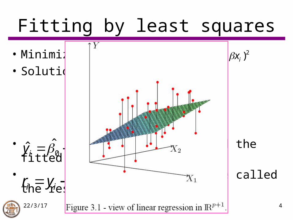
Fitting by least squares
• Minimize:
• Solutions are
• are called the fitted or predicted values
• are called the residuals
N
i ii xy1
20,0 )(minargˆ,ˆ
0
xy
xx
yxxN
j i
N
j ii
ˆˆ)(
)(ˆ
0
1
2
1
ii xy ˆˆˆ 0
iii xyr ˆˆ0
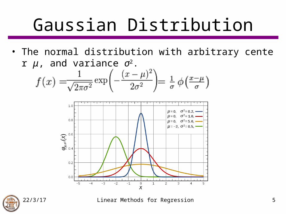
Gaussian Distribution• The normal distribution with arbitrary center μ, and variance
σ2.
23/4/18 Linear Methods for Regression 5
23/4/18 Linear Methods for Regression 6
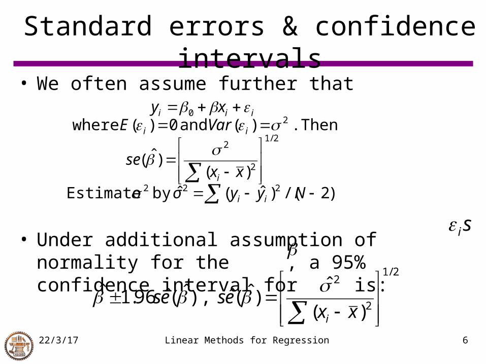
Standard errors & confidence intervals• We often assume further that
• Under additional assumption of normality for the , a 95% confidence interval for is:
).2/()ˆ(ˆ)(
)ˆ(
)(0)(
222
2/1
2
2
20
Nyyσxx
se
VarExy
ii
i
ii
iii
by Estimate
.Then and where
si
2/1
2
2
)(
ˆ)ˆ(ˆ),ˆ(ˆ96.1ˆ
xxeses
i
23/4/18 Linear Methods for Regression 7
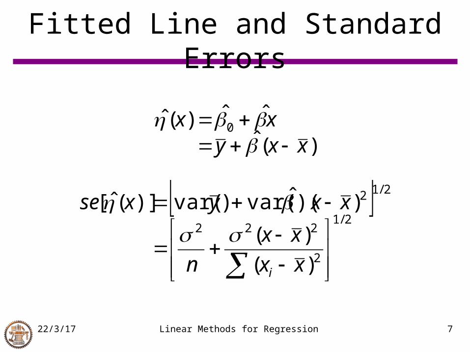
Fitted Line and Standard Errors
)(ˆˆˆ)(ˆ 0
xxyxx
2/1
2
222
2/12
)(
)(
))(ˆvar()var()](ˆ[
xx
xx
n
xxyxse
i
23/4/18 Linear Methods for Regression 8
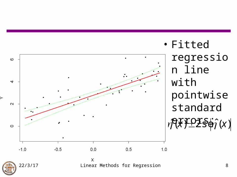
• Fitted regression line with pointwise standard errors:
)(ˆse2)(ˆ xx
23/4/18 Linear Methods for Regression 9
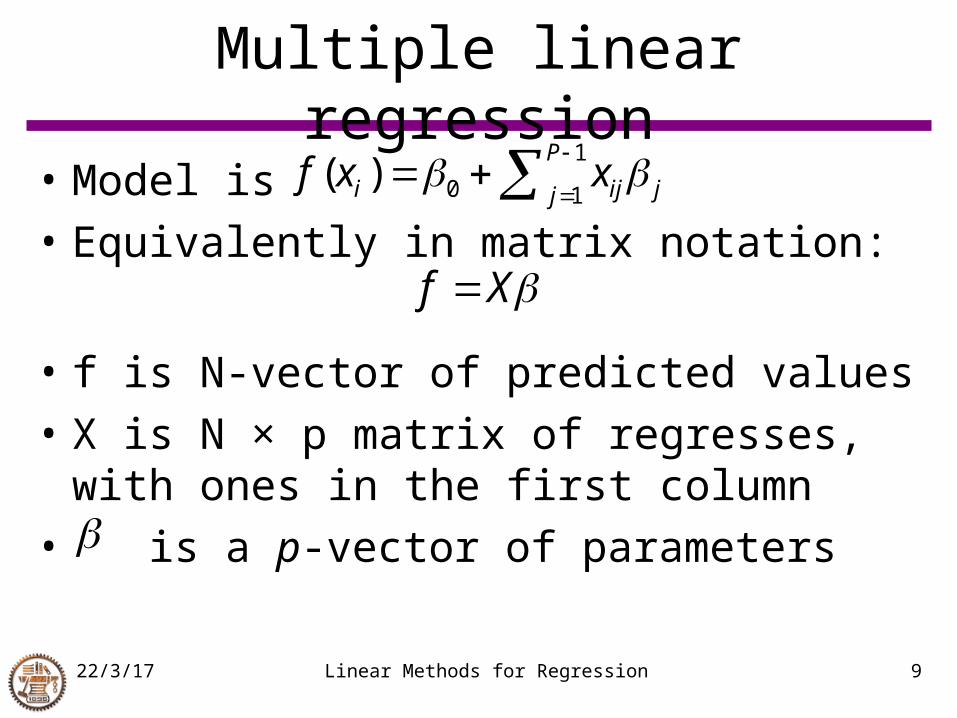
Multiple linear regression
• Model is
• Equivalently in matrix notation:
• f is N-vector of predicted values
• X is N × p matrix of regresses, with ones in the first column
• is a p-vector of parameters
1
0 1( )
P
i ij jjf x x
Xf
23/4/18 Linear Methods for Regression 10
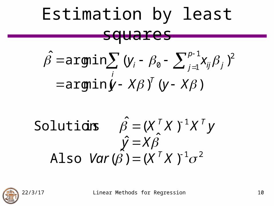
Estimation by least squares
)()min(arg
)(minargˆ 21
10
XyXy
xy
Ti
p
j jiji
21
1
)()ˆ(
ˆˆ)(ˆ
XXVarXy
yXXX
T
TT
Also
is Solution
23/4/18 Linear Methods for Regression 11
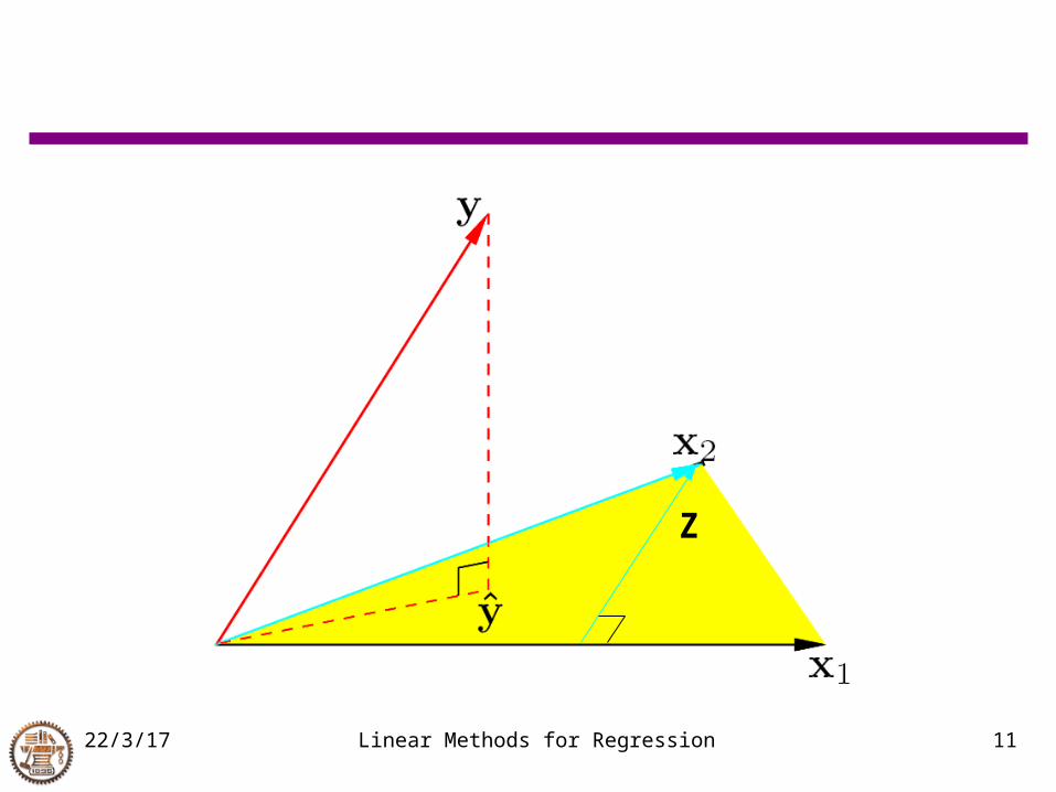
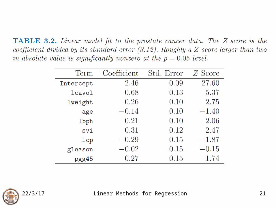
Z
23/4/18 Linear Methods for Regression 12
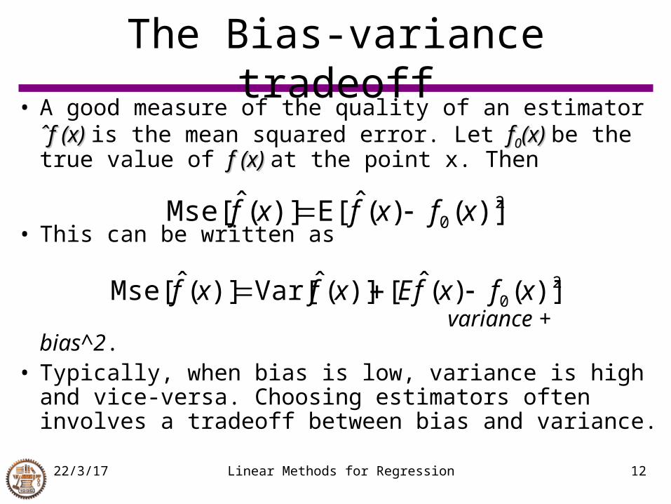
The Bias-variance tradeoff• A good measure of the quality of an estimator ˆf (x) ˆf (x)
is the mean squared error. Let ff00(x) (x) be the true value of f (x) f (x) at the point x. Then
• This can be written as
variance + bias^2.• Typically, when bias is low, variance is high and
vice-versa. Choosing estimators often involves a tradeoff between bias and variance.
20 )]()(ˆE[)](ˆMse[ xfxfxf
20 )]()(ˆ[)](ˆVar[)](ˆMse[ xfxfExfxf
23/4/18 Linear Methods for Regression 13
The Bias-variance tradeoff
• If the linear model is correct for a given problem, then the least squares prediction f is unbiased, and has the lowest variance among all unbiased estimators that are linear functions of y.
• But there can be (and often exist) biased estimators with smaller MSE.
• Generally, by regularizing (shrinking, dampening, controlling) the estimator in some way, its variance will be reduced; if the corresponding increase in bias is small, this will be worthwhile.
23/4/18 Linear Methods for Regression 14
The Bias-variance tradeoff
• Examples of regularization: subset selection (forward, backward, all subsets); ridge regression, the lasso.
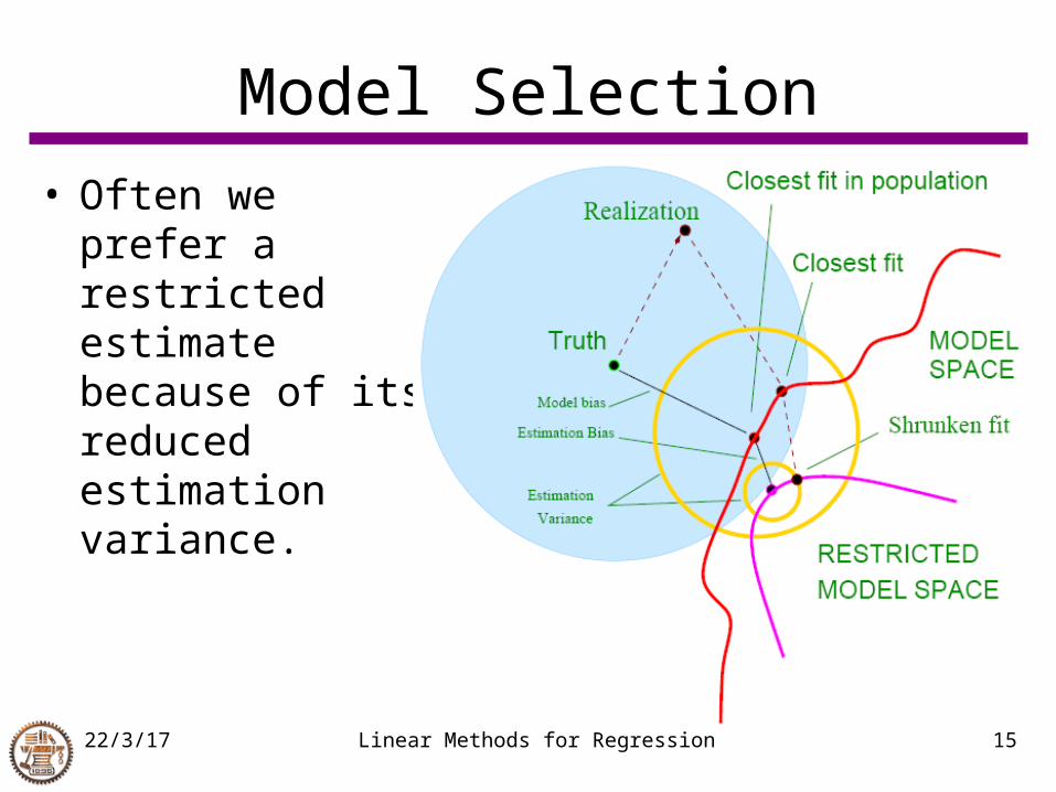
• In reality models are almost never correct, so there is an additional model bias between the closest member of the linear model class and the truth.
23/4/18 Linear Methods for Regression 15
Model Selection
• Often we prefer a restricted estimate because of its reduced estimation variance.
23/4/18 Linear Methods for Regression 16
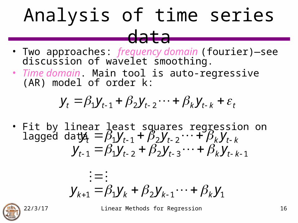
Analysis of time series data• Two approaches: frequency domain (fourier)—see
discussion of wavelet smoothing.• Time domain. Main tool is auto-regressive (AR) model of
order k:
• Fit by linear least squares regression on lagged data
tktkttt yyyy 2211
11211
132211
2211
yyyy
yyyyyyyy
kkkk
ktkttt
ktkttt
23/4/18 Linear Methods for Regression 17
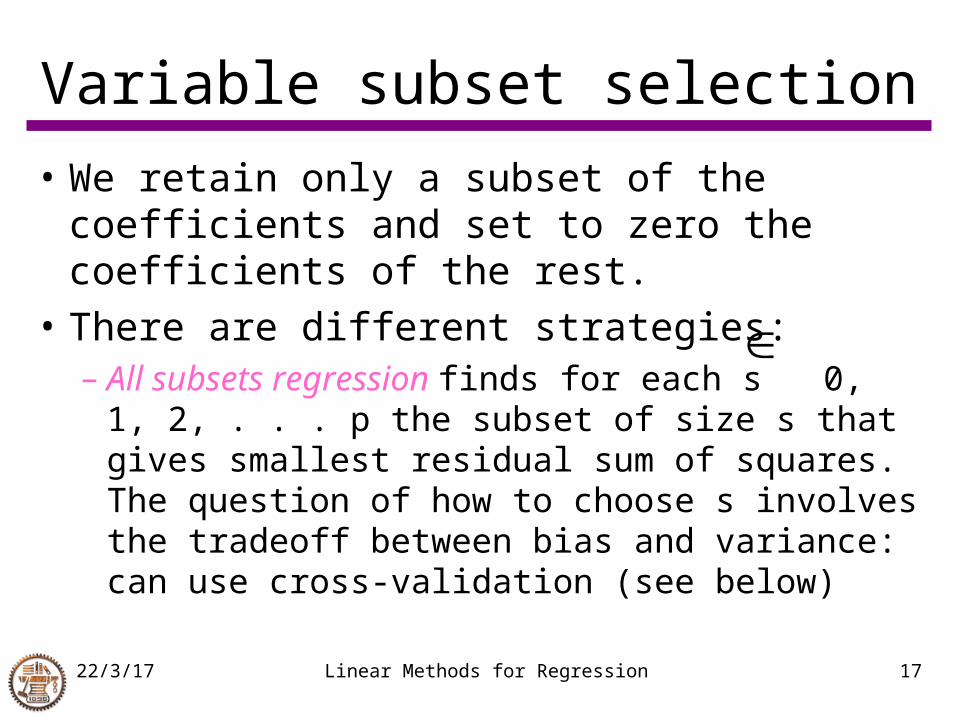
Variable subset selection
• We retain only a subset of the coefficients and set to zero the coefficients of the rest.
• There are different strategies:– All subsets regression finds for each s 0, 1,
2, . . . p the subset of size s that gives smallest residual sum of squares. The question of how to choose s involves the tradeoff between bias and variance: can use cross-validation (see below)
23/4/18 Linear Methods for Regression 18
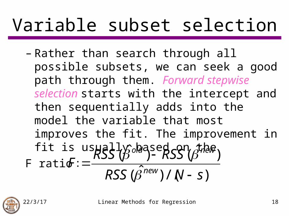
Variable subset selection
– Rather than search through all possible subsets, we can seek a good path through them. Forward stepwise selection starts with the intercept and then sequentially adds into the model the variable that most improves the fit. The improvement in fit is usually based on the
F ratio:
)/()ˆ(
)ˆ()ˆ(
sNRSS
RSSRSSF
new
newold
23/4/18 Linear Methods for Regression 19
23/4/18 Linear Methods for Regression 20
23/4/18 Linear Methods for Regression 21
23/4/18 Linear Methods for Regression 22
Variable subset selection
• Backward stepwise selection starts with the full OLS model, and sequentially deletes variables.
• There are also hybrid stepwise selection strategies which add in the best variable and delete the least important variable, in a sequential manner.
• Each procedure has one or more tuning parameters:
– subset size
– P-valuesP-values for adding or dropping terms
23/4/18 Linear Methods for Regression 23
Model Assessment• Objectives:
1. Choose a value of a tuning parameter for a technique
2. Estimate the prediction performance of a given model
• For both of these purposes, the best approach is to run the procedure on an independent test set, if one is available
• If possible one should use different test data for (1) and (2) above: a validation set for (1) and a test set for (2)
• Often there is insufficient data to create a separate validation or test set. In this instance Cross-Validation is useful.
23/4/18 Linear Methods for Regression 24
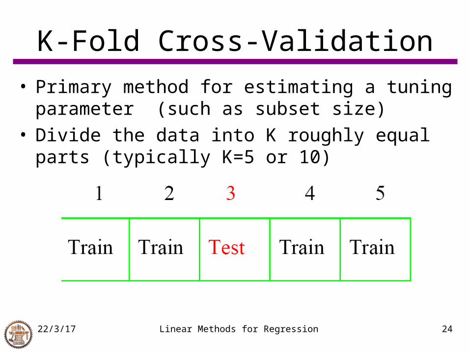
K-Fold Cross-Validation
• Primary method for estimating a tuning parameter (such as subset size)
• Divide the data into K roughly equal parts (typically K=5 or 10)
23/4/18 Linear Methods for Regression 25
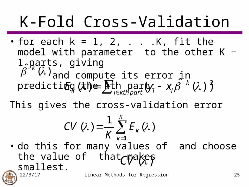
K-Fold Cross-Validation• for each k = 1, 2, . . .K, fit the model with
parameter to the other K − 1 parts, giving and compute its error in predicting
the kth part:
This gives the cross-validation error
• do this for many values of and choose the value of that makes smallest.
)(ˆ k
partkthi
kiik xyE 2))(ˆ()(
K
kkE
KCV
1
)(1
)(
)(CV
23/4/18 Linear Methods for Regression 26
K-Fold Cross-Validation
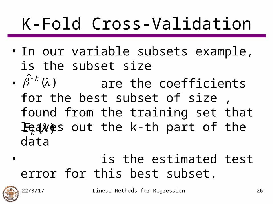
• In our variable subsets example, is the subset size
• are the coefficients for the best subset of size , found from the training set that leaves out the k-th part of the data
• is the estimated test error for this best subset.
)(ˆ k
)(kE
23/4/18 Linear Methods for Regression 27
K-Fold Cross-Validation
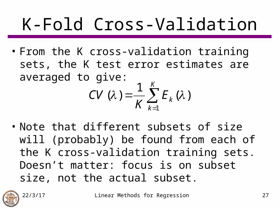
• From the K cross-validation training sets, the K test error estimates are averaged to give:
• Note that different subsets of size will (probably) be found from each of the K cross-validation training sets. Doesn’t matter: focus is on subset size, not the actual subset.
K
kkE
KCV
1
)(1
)(
23/4/18 Linear Methods for Regression 28
The Bootstrap approach• Bootstrap works by sampling N times with
replacement from training set to form a “bootstrap” data set. Then model is estimated on bootstrap data set, and predictions are made for original training set.
• This process is repeated many times and the results are averaged.
• Bootstrap most useful for estimating standard errors of predictions.
• Sometimes produces better estimates than cross-validation (topic for current research)
23/4/18 Linear Methods for Regression 29
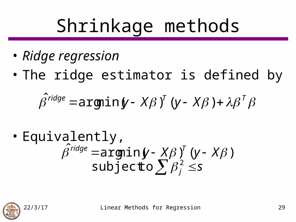
Shrinkage methods
• Ridge regression
• The ridge estimator is defined by
• Equivalently,
TTridge XyXy )()min(argˆ
sXyXy
j
Tridge
2)()min(argˆ
to subject
23/4/18 Linear Methods for Regression 30
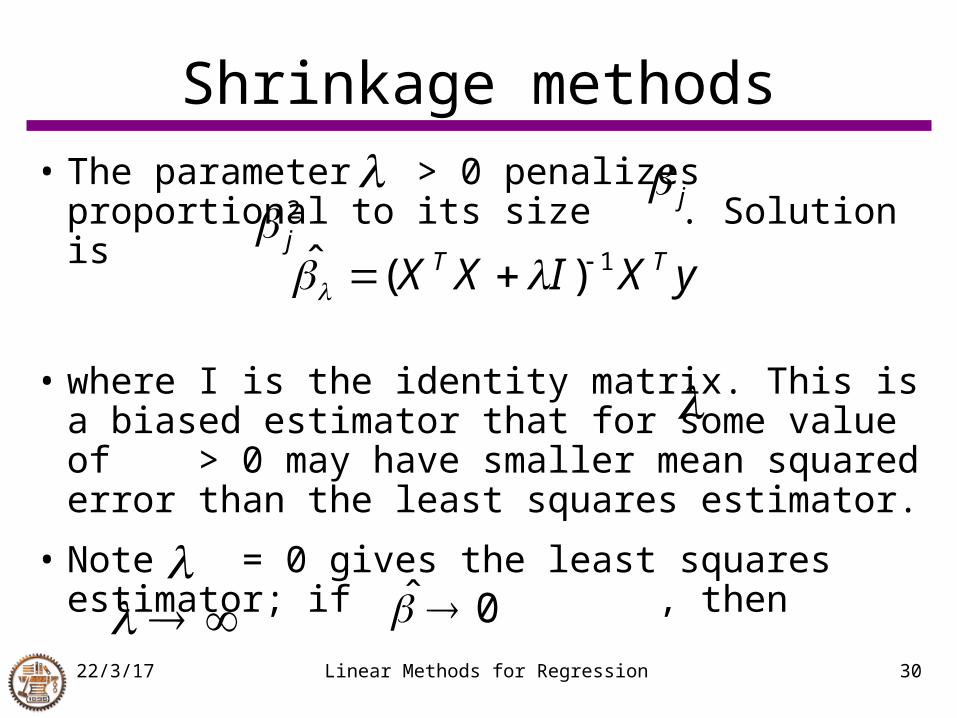
Shrinkage methods
• The parameter > 0 penalizes proportional to its size . Solution is
• where I is the identity matrix. This is a biased estimator that for some value of > 0 may have smaller mean squared error than the least squares estimator.
• Note = 0 gives the least squares estimator; if , then
j
2j
yXIXX TT 1)(ˆ
0ˆ
23/4/18 Linear Methods for Regression 31
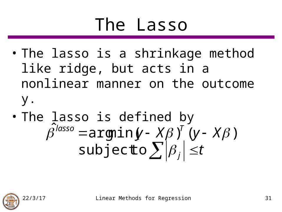
The Lasso
• The lasso is a shrinkage method like ridge, but acts in a nonlinear manner on the outcome y.
• The lasso is defined by
t
XyXy
j
Tlasso
to subject)()min(argˆ
23/4/18 Linear Methods for Regression 32
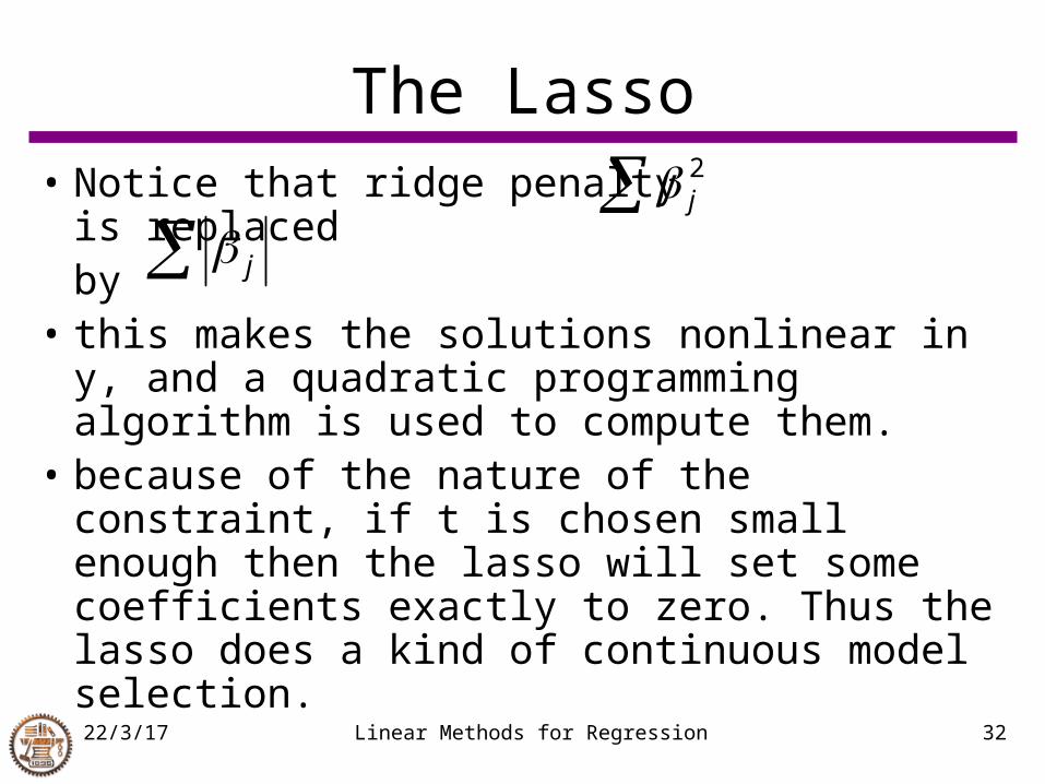
The Lasso• Notice that ridge penalty is replaced
by• this makes the solutions nonlinear in y, and a
quadratic programming algorithm is used to compute them.
• because of the nature of the constraint, if t is chosen small enough then the lasso will set some coefficients exactly to zero. Thus the lasso does a kind of continuous model selection.
j 2
j
23/4/18 Linear Methods for Regression 33
The Lasso
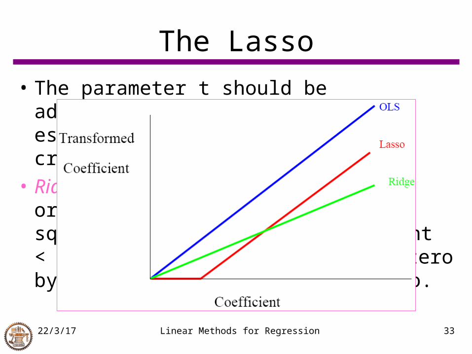
• The parameter t should be adaptively chosen to minimize an estimate of expected, using say cross-validation
• Ridge vs Lasso: if inputs are orthogonal, ridge multiplies least squares coefficients by a constant < 1, lasso translates them towards zero by a constant, truncating at zero.
23/4/18 Linear Methods for Regression 34
A family of shrinkage estimators
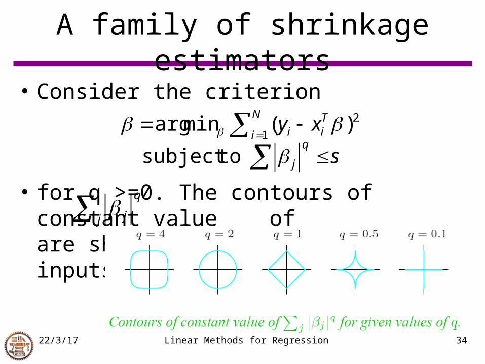
• Consider the criterion
• for q >=0. The contours of constant value of are shown for the case of two inputs.
s
xyq
j
N
i
Tii
to subject1
2)(minarg
j
q
j
23/4/18 Linear Methods for Regression 35
Use of derived input directions
• Principal components regression• We choose a set of linear combinations of the xj s,
and then regress the outcome on these linear combinations.
• The particular combinations used are the sequence of principal components of the inputs. These are uncorrelated and ordered by decreasing variance.
• If S is the sample covariance matrix of , then the eigenvector equations
define the principal components of S.ljl qdSq 2
1 2,, , px x x
23/4/18 Linear Methods for Regression 36
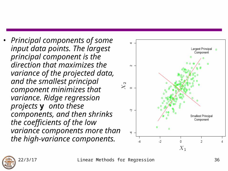
• Principal components of some input data points. The largest principal component is the direction that maximizes the variance of the projected data, and the smallest principal component minimizes that variance. Ridge regression projects y onto these components, and then shrinks the coefficients of the low variance components more than the high-variance components.
23/4/18 Linear Methods for Regression 37
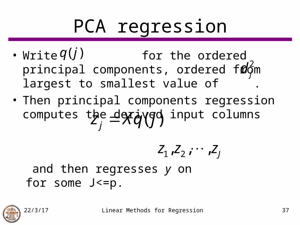
PCA regression
• Write for the ordered principal components, ordered from largest to smallest value of .
• Then principal components regression computes the derived input columns
and then regresses y on for some J<=p.
2jd
( )q j
( )jz Xq j
1 2, , , Jz z z
23/4/18 Linear Methods for Regression 38
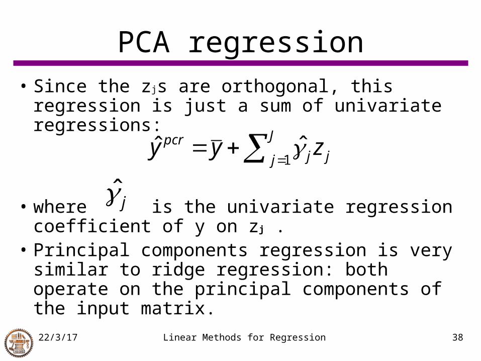
PCA regression
• Since the zjs are orthogonal, this regression is just a sum of univariate regressions:
• where is the univariate regression coefficient of y on zj .
• Principal components regression is very similar to ridge regression: both operate on the principal components of the input matrix.
J
j jjpcr zyy
1ˆˆ
j
23/4/18 Linear Methods for Regression 39
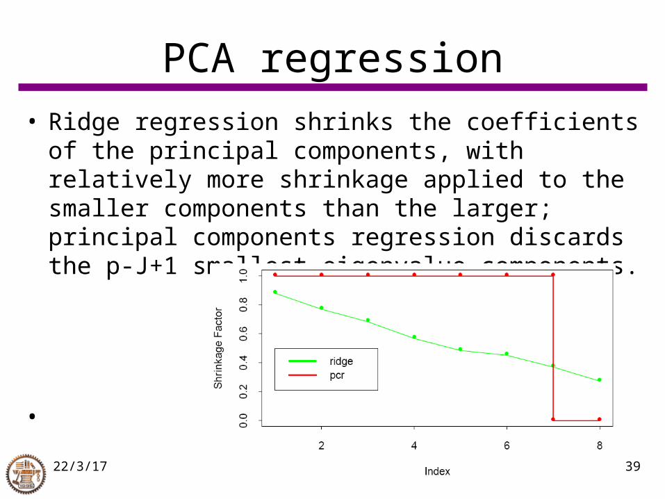
PCA regression
• Ridge regression shrinks the coefficients of the principal components, with relatively more shrinkage applied to the smaller components than the larger; principal components regression discards the p-J+1 smallest eigenvalue components.
•
23/4/18 Linear Methods for Regression 40
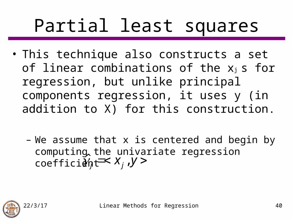
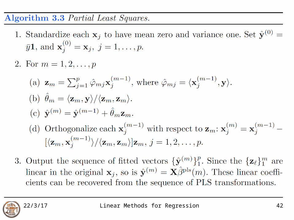
Partial least squares
• This technique also constructs a set of linear combinations of the xj s for regression, but unlike principal components regression, it uses y (in addition to X) for this construction.
– We assume that x is centered and begin by computing the univariate regression coefficient
ˆ ,j jx y
23/4/18 Linear Methods for Regression 41
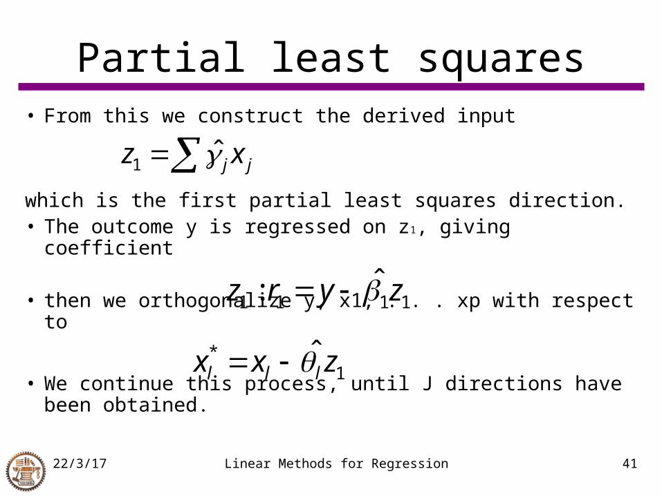
Partial least squares• From this we construct the derived input
which is the first partial least squares direction.• The outcome y is regressed on z1, giving coefficient
• then we orthogonalize y, x1, . . . xp with respect to
• We continue this process, until J directions have been obtained.
jj xz 1
1111ˆ: zyrz
1* ˆ zxx lll
23/4/18 Linear Methods for Regression 42
23/4/18 Linear Methods for Regression 43
Ridge vs PCR vs PLS vs Lasso
• Recent study has shown that ridge and PCR outperform PLS in prediction, and they are simpler to understand.
• Lasso outperforms ridge when there are a moderate number of sizable effects, rather than many small effects. It also produces more interpretable models.
• These are still topics for ongoing research.


