29
EE103 (Fall 2011-12) 18. Linear optimization • linear program • examples • geometrical interpretation • extreme points • simplex method 18-1
| Date post: | 17-Jul-2016 |
| Category: |
Documents |
| Upload: | bhuvana-vignaesh |
| View: | 221 times |
| Download: | 3 times |

EE103 (Fall 2011-12)
18. Linear optimization
• linear program
• examples
• geometrical interpretation
• extreme points
• simplex method
18-1

Linear program
minimize c1x1 + c2x2 + · · ·+ cnxn
subject to a11x1 + a12x2 + · · ·+ a1nxn ≤ b1a21x1 + a22x2 + · · ·+ a2nxn ≤ b2· · ·am1x1 + am2x2 + · · ·+ amnxn ≤ bm
• n optimization (decision) variables x1, . . . , xn
• m linear inequality constraints
matrix notation
minimize cTxsubject to Ax ≤ b
the inequality between vectors Ax ≤ b is interpreted elementwise
Linear optimization 18-2

Production planning
• a company makes three products, in quantities x1, x2, x3 per month
• profit per unit is 1.0 (for product 1), 1.4 (product 2), 1.6 (product 3)
• products use different amounts of resources (labor, material, . . . )
fraction of total available resource needed per unit of each product
product 1 product 2 product 3
resource 1 1/1000 1/800 1/500
resource 2 1/1200 1/700 1/600
optimal production plan
maximize x1 + 1.4x2 + 1.6x3
subject to (1/1000)x1 + (1/800)x2 + (1/500)x3 ≤ 1(1/1200)x1 + (1/700)x2 + (1/600)x3 ≤ 1x1 ≥ 0, x2 ≥ 0, x3 ≥ 0
solution: x1 = 462, x2 = 431, x3 = 0
Linear optimization 18-3

Network flow optimization
t t1
2
3
4
5
6
x1
x2
x3
x4
x5
x6
x7
x8
x9
capacityconstraints
0 ≤ x1 ≤ 30 ≤ x2 ≤ 20 ≤ x3 ≤ 10 ≤ x4 ≤ 20 ≤ x5 ≤ 10 ≤ x6 ≤ 30 ≤ x7 ≤ 30 ≤ x8 ≤ 10 ≤ x9 ≤ 1
maximize tsubject to flow conservation at nodes
capacity constraints on the arcs
Linear optimization 18-4

linear programming formulation
maximize tsubject to t = x1 + x2, x1 + x3 = x4, et cetera
0 ≤ x1 ≤ 3, 0 ≤ x2 ≤ 2, et cetera
(t = x1 + x2 is equivalent to inequalities t ≤ x1 + x2, t ≥ x1 + x2, . . . )
solution
4 41
2
3
4
5
6
2
2
2
2
3
1
1
Linear optimization 18-5

Data fitting
fit a straight line to m points (ui, vi) by minimizing sum of absolute errors
minimize
m∑
i=1
|α+ βui − vi|
−10 −5 0 5 10−15
−10
−5
0
5
10
15
20
u
v
dashed: least-squares solution; solid: minimizes sum of absolute errors
Linear optimization 18-6

linear programming formulation
minimize
m∑
i=1
yi
subjec to −yi ≤ α+ βui − vi ≤ yi, i = 1, . . . ,m
• variables α, β, y1, . . . , ym
• inequalities are equivalent to
yi ≥ |α+ βui − vi|
• the optimal yi satisfies
yi = |α+ βui − yi|
Linear optimization 18-7

Terminology
minimize cTxsubject to Ax ≤ b
problem data: n-vector c, m× n-matrix A, m-vector b
• x is feasible if Ax ≤ b
• feasible set is set of all feasible points
• x⋆ is optimal if it is feasible and cTx⋆ ≤ cTx for all feasible x
• optimal value: p⋆ = cTx⋆
• unbounded problem: cTx is unbounded below on feasible set
• infeasible probem: feasible set is empty
Linear optimization 18-8

Example
minimize −x1 − x2
subject to 2x1 + x2 ≤ 3x1 + 4x2 ≤ 5x1 ≥ 0, x2 ≥ 0
x1
x2
2x1 + x2 = 3
x1 + 4x2 = 5
feasible set is shaded
Linear optimization 18-9

solutionminimize −x1 − x2
subject to 2x1 + x2 ≤ 3x1 + 4x2 ≤ 5x1 ≥ 0, x2 ≥ 0
x1
x2
−x1 − x2 = 0
−x1 − x2 = −1
−x1 − x2 = −2
−x1 − x2 = −3
−x1 − x2 = −4
−x1 − x2 = −5
optimal solution is x⋆ = (1, 1), optimal value is p⋆ = −2
Linear optimization 18-10

Hyperplanes and halfspaces
hyperplane
solution set of one linear equation with nonzero coefficient vector a
aTx = b
halfspace
solution set of one linear inequality with nonzero coefficient vector a
aTx ≤ b
Linear optimization 18-11

Geometrical interpretation
G = {x | aTx = b} H = {x | aTx ≤ b}
a
u = (b/‖a‖2)a
x
x − u
0
G
a
xu
x − u H
• u = (b/‖a‖2)a satisfies aTu = b
• x is in G if aT (x− u) = 0, i.e., x− u is orthogonal to a
• x is in H if aT (x− u) ≤ 0, i.e., angle 6 (x− u, a) ≥ π/2
Linear optimization 18-12

Example
a = (2, 1)
x1
x2
aTx = −5
aTx = 10
aTx = 5
aTx = 0
a = (2, 1)
x1
x2
aTx ≤ 3
Linear optimization 18-13

Polyhedron
definition: the solution set of a finite number of linear inequalities
aT1 x ≤ b1, aT2 x ≤ b2, . . . , aTmx ≤ bm
matrix notation: Ax ≤ b where
A =
aT1aT2...aTm
, b =
b1b2...bm
geometrical interpretation: intersection of m halfspaces
Linear optimization 18-14

example (n = 2)
x1 + x2 ≥ 1, −2x1 + x2 ≤ 2, x1 ≥ 0, x2 ≥ 0
x1
x2
x1 + x2 = 1
−2x1 + x2 = 2
Linear optimization 18-15

example (n = 3)
0 ≤ x1 ≤ 2, 0 ≤ x2 ≤ 2, 0 ≤ x3 ≤ 2, x1 + x2 + x3 ≤ 5
x1
x2
x3
(2, 0, 0)
(2, 0, 2)
(0, 0, 2) (0, 2, 2)
(0, 2, 0)
(2, 2, 0)
(2, 2, 1)
(2, 1, 2)
(1, 2, 2)
Linear optimization 18-16

Extreme points
let x̂ ∈ P, where P is a polyhedron defined by inequalities aTk x ≤ bk
• if aTk x̂ = bk, we say the kth inequality is active at x̂
• if aTk x̂ < bk, we say the kth inequality is inactive at x̂
x̂ is called an extreme point of P if
AI(x̂) =
aTk1aTk2...aTkp
has a zero nullspace
where I(x̂) = {k1, . . . , kp} are the indices of the active constraints at x̂
an extreme point x̂ is nondegenerate if p = n, degenerate if p > n
Linear optimization 18-17
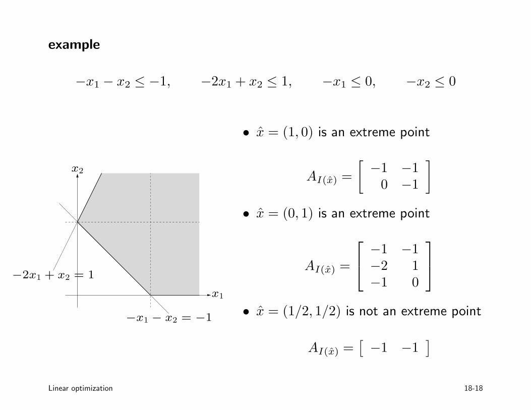
example
−x1 − x2 ≤ −1, −2x1 + x2 ≤ 1, −x1 ≤ 0, −x2 ≤ 0
x1
x2
−x1 − x2 = −1
−2x1 + x2 = 1
• x̂ = (1, 0) is an extreme point
AI(x̂) =
[
−1 −10 −1
]
• x̂ = (0, 1) is an extreme point
AI(x̂) =
−1 −1−2 1−1 0
• x̂ = (1/2, 1/2) is not an extreme point
AI(x̂) =[
−1 −1]
Linear optimization 18-18

Simplex algorithm
minimize x1 + x2 − x3
subject to 0 ≤ x1 ≤ 2, 0 ≤ x2 ≤ 2, 0 ≤ x3 ≤ 2x1 + x2 + x3 ≤ 5
x1
x2
x3
(0, 0, 2)
(2, 2, 0)
move from one extreme point to another extreme point with lower cost
Linear optimization 18-19
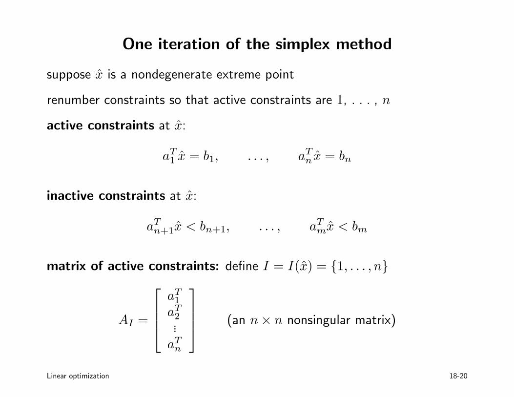
One iteration of the simplex method
suppose x̂ is a nondegenerate extreme point
renumber constraints so that active constraints are 1, . . . , n
active constraints at x̂:
aT1 x̂ = b1, . . . , aTn x̂ = bn
inactive constraints at x̂:
aTn+1x̂ < bn+1, . . . , aTmx̂ < bm
matrix of active constraints: define I = I(x̂) = {1, . . . , n}
AI =
aT1aT2...aTn
(an n× n nonsingular matrix)
Linear optimization 18-20

step 1 (test for optimality) solve
ATI z = c
i.e., find z that satisfiesn∑
k=1
zkak = c
if zk ≤ 0 for all k, then x̂ is optimal and we return x̂
proof. consider any feasible x:
cTx =
n∑
k=1
zkaTk x ≥
n∑
k=1
zkbk =
n∑
k=1
zkaTk x̂ = cT x̂
(the inequality follows from zk ≤ 0, aTk x ≤ bk)
Linear optimization 18-21

step 2 (compute step) choose a j with zj > 0 and solve
AIv = −ej
i.e., find v that satisfies
aTj v = −1, aTk v = 0 for k = 1, . . . , n and k 6= j
for small t > 0, x̂+ tv is feasible and has a smaller cost than x̂
proof:
aTj (x̂+ tv) = bj − t
aTk (x̂+ tv) = bk for k = 1, . . . , n and k 6= j
and for sufficiently small positive t
aTk (x̂+ tv) ≤ bk for k = n+ 1, . . . ,m
finally, cT (x̂+ tv) = cT x̂+ tzj < cT x̂
Linear optimization 18-22

step 3 (compute step size) maximum t such that x̂+ tv is feasible, i.e.,
aTk x̂+ taTk v ≤ bk, k = 1, . . . ,m
the maximum step size is
tmax = mink:aT
kv>0
bk − aTk x̂
aTk v
(if aTk v ≤ 0 for all k, then the problem is unbounded below)
step 4 (update x̂)
x̂ := x̂+ tmaxv
Linear optimization 18-23

Example
minimize x1 + x2 − x3
subject to 0 ≤ x1 ≤ 2, 0 ≤ x2 ≤ 2, 0 ≤ x3 ≤ 2x1 + x2 + x3 ≤ 5
at x̂ = (2, 2, 0)
AI =
1 0 00 1 00 0 −1
1. z = A−TI c = (1, 1, 1)
2. for j = 3, v = A−1I (0, 0,−1) = (0, 0, 1)
3. x̂+ tv is feasible for t ≤ 1 x1
x2
x3
(2, 2, 0)
(2, 2, 1)
Linear optimization 18-24

Example
minimize x1 + x2 − x3
subject to 0 ≤ x1 ≤ 2, 0 ≤ x2 ≤ 2, 0 ≤ x3 ≤ 2x1 + x2 + x3 ≤ 5
at x̂ = (2, 2, 1)
AI =
1 0 00 1 01 1 1
1. z = A−TI c = (2, 2,−1)
2. for j = 2, v = A−1I (0,−1, 0) = (0,−1, 1)
3. x̂+ tv is feasible for t ≤ 1 x1
x2
x3
(2, 2, 1)
(2, 1, 2)
Linear optimization 18-25

Example
minimize x1 + x2 − x3
subject to 0 ≤ x1 ≤ 2, 0 ≤ x2 ≤ 2, 0 ≤ x3 ≤ 2x1 + x2 + x3 ≤ 5
at x̂ = (2, 1, 2)
AI =
1 0 00 0 11 1 1
1. z = A−TI c = (0,−2, 1)
2. for j = 3, v = A−1I (−1, 0, 0) = (0,−1, 0)
3. x̂+ tv is feasible for t ≤ 1 x1
x2
x3
(2, 0, 2) (2, 1, 2)
Linear optimization 18-26

Example
minimize x1 + x2 − x3
subject to 0 ≤ x1 ≤ 2, 0 ≤ x2 ≤ 2, 0 ≤ x3 ≤ 2x1 + x2 + x3 ≤ 5
at x̂ = (2, 0, 2)
AI =
1 0 00 −1 00 0 1
1. z = A−TI c = (1,−1,−1)
2. for j = 1, v = A−1I (−1, 0, 0) = (−1, 0, 0)
3. x̂+ tv is feasible for t ≤ 2 x1
x2
x3
(2, 0, 2)
(0, 0, 2)
Linear optimization 18-27

Example
minimize x1 + x2 − x3
subject to 0 ≤ x1 ≤ 2, 0 ≤ x2 ≤ 2, 0 ≤ x3 ≤ 2x1 + x2 + x3 ≤ 5
at x̂ = (0, 0, 2)
AI =
−1 0 00 −1 00 0 1
z = A−TI c = (−1,−1,−1)
therefore, x̂ is optimal
x1
x2
x3
(0, 0, 2)
Linear optimization 18-28

Practical aspects
• at each iteration, we solve two sets of linear equations
ATI z = c, AIv = −ej
using an LU factorization or sparse LU factorization of AI
• implementation requires a ‘phase 1’ to find first extreme point
• simple modifications handle problems with degenerate extreme points
• very large LPs (several 100,000 variables and constraints) are routinelysolved in practice
Linear optimization 18-29


