23
Linear Programming Linear Programming
| Date post: | 21-Dec-2015 |
| Category: |
Documents |
| View: | 222 times |
| Download: | 0 times |

Linear ProgrammingLinear ProgrammingLinear ProgrammingLinear Programming

Linear programmingLinear programmingLinear programmingLinear programming
A technique that allows decision A technique that allows decision
makers to solvemakers to solve maximization maximization and and
minimization minimization problems where there are problems where there are
certain certain constraintsconstraints that limit what can that limit what can
be done, given that all objectives and be done, given that all objectives and
constraints areconstraints are linear linear..

DefinitionsDefinitionsDefinitionsDefinitions
The The objective functionobjective function is the function to be is the function to be maximized (or minimized)maximized (or minimized)
TheThe constraintsconstraints are given in inequalities.are given in inequalities.
Both the Both the objective objective and and constraintsconstraints are are
linearlinear in choice variables in choice variables

ExampleExampleExampleExample
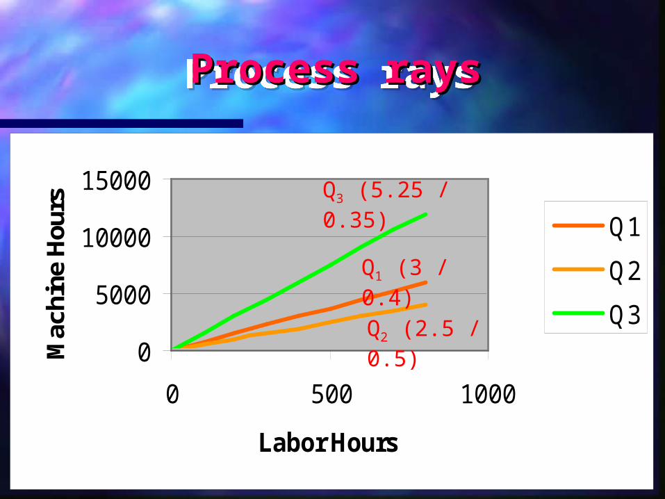
Process 1:Process 1: requires requires 33 machine-hours and machine-hours and 0.40.4 labor-hours per batch of cloth.labor-hours per batch of cloth.
Process 2:Process 2: requires requires 2.52.5 machine-hours and machine-hours and 0.50.5 labor-hours per batch of cloth.labor-hours per batch of cloth.
Process 3:Process 3: requires requires 5.255.25 machine-hours and machine-hours and 0.350.35 labor-hours per batch of cloth. labor-hours per batch of cloth.
The profit isThe profit is $1 $1, , $0.9$0.9, and , and $1.1$1.1 with process with process 11, , 22, , andand 33, respectively., respectively.
Max Max LL and and KK are are 600600 and and 6,0006,000, respectively., respectively.

The objective is to maximize profit subject to resource constraints
Maximize = 1.0Q1 + 0.9Q2 + 1.1Q3
subject to the constraints:
3Q1 + 2.5Q2 + 5.25Q3 ≦ 6000 (Machine hours)
0.4Q1 + 0.5Q2 + 0.35Q3 ≦ 600 (Labor Hours)
Q1 ≧ 0; Q2 ≧ 0; Q3 ≧ 0
Process raysProcess raysProcess raysProcess rays
0
5000
10000
15000
0 500 1000
Labor Hours
Mac
hine
Hou
rs
Q1
Q2
Q3
Q3 (5.25 / 0.35)
Q1 (3 / 0.4)
Q2 (2.5 / 0.5)

0
5000
10000
15000
0 500 1000
Labor Hours
Mac
hine
Hou
rs Q1
Q2
Q3
Isoquants (line ABC, NOT line AC)
A
BC
Q3 (5.25 / 0.35)
Q1 (3 / 0.4)
Q2 (2.5 / 0.5)

Feasible SetFeasible SetFeasible SetFeasible Set
0
5000
10000
15000
0 500 1000
Labor Hours
Mac
hin
e H
ou
rs
Q1
Q2
Q3
(6000, 600)
Q2 (2.5 / 0.5)
Q1 (3 / 0.4)
Q3 (5.25 / 0.35)

Graphical Solution:Graphical Solution: A*A*
0
5000
10000
15000
0 500 1000
Labor Hours
Mac
hin
e H
ou
rs
Q1
Q2
Q3
A*
Q3 (5.25 / 0.35)
Q1 (3 / 0.4)
Q2 (2.5 / 0.5)

Suppose that the company is no longer Suppose that the company is no longer constrained by limits on the amount of Labor constrained by limits on the amount of Labor and capital.and capital.
It can hire all ofIt can hire all of labor labor it wants at it wants at $12 $12 per hour and per hour and all of the all of the capitalcapital at at $1.6$1.6 per machine-hour. per machine-hour.
Its problem is to choose that combination of Its problem is to choose that combination of processes which will produce, say, 400 units at processes which will produce, say, 400 units at minimum minimum cost.cost.
MinMin C = C = 9.69.6 Q Q1 1 + + 1010 Q Q22 + + 12.612.6 Q Q33
Subject toSubject to: Q: Q1 1 + Q+ Q22 + Q + Q3 3 ≧≧ 400 400
QQ1 1 ≧≧ 0, Q 0, Q22 ≧≧ 0, Q 0, Q3 3 ≧ ≧ 0 0

Optimal Solution: Cost Minimization Problem
0
5000
10000
15000
0 500 1000
Labor Hours
Mac
hine
Hou
rs
Q1
Q2
Q3
B*
Iso-cost line Q3 (5.25 / 0.35)
Q1 (3 / 0.4)
Q2 (2.5 / 0.5)
Solution: All of the output are produced with process 1

Simplex methodSimplex methodSimplex methodSimplex method
A systematic process for A systematic process for
comparing comparing extreme pointextreme point or or corner corner
solutionssolutions to linear programming to linear programming
problemsproblems

Dual problemsDual problemsDual problemsDual problems
Every optimization problem has a Every optimization problem has a corresponding problem called its corresponding problem called its dualdual
If the If the primalprimal problem is a problem is a maximizationmaximization, , the the dualdual is a is a minimizationminimization (and (and vice versavice versa))
Solutions to the dual are Solutions to the dual are shadow pricesshadow prices

Shadow PricesShadow PricesShadow PricesShadow Prices
Shadow prices tell you what would happen to the Shadow prices tell you what would happen to the objectiveobjective functionfunction if you relaxed the constraint by if you relaxed the constraint by one unitone unit..
They show which types of capacity are They show which types of capacity are bottlenecksbottlenecks, , or or effective constraintseffective constraints on output, since capacity on output, since capacity that is that is underutilizedunderutilized receives a receives a zerozero shadow price. shadow price.
More important, shadow prices indicate how much More important, shadow prices indicate how much it would be it would be worthworth to management to expand each to management to expand each type of capacity. type of capacity.

ExampleExample
Output 1 (Q1 ): requires 3 units of capital and 2
units of labor to produce one unit of output 1.
Output 2 (Q2 ): requires 5 units of capital and 4
units of labor to produce one unit of output 2.
The firm has 4,000 units of labor and 5,400 units of capital.
The price of Q1 and Q2 are $50 and $80, respectively.

Primal problemPrimal problemPrimal problemPrimal problem
The primal problem is to find the value of The primal problem is to find the value of QQ11 and and QQ22
that that maximize total revenuemaximize total revenue subject to the subject to the resource resource
constraintconstraint..
Max TR = 50 Max TR = 50 QQ11 + 80 + 80 QQ22
Subject to: 2Subject to: 2QQ11 + 4 + 4 QQ2 2 ≦≦ 4,0004,000
33QQ11 + 5 + 5 QQ22 ≦≦ 5,4005,400
QQ11 ≧≧ 0, Q0, Q22 ≧≧ 0 0
Dual problemDual problem
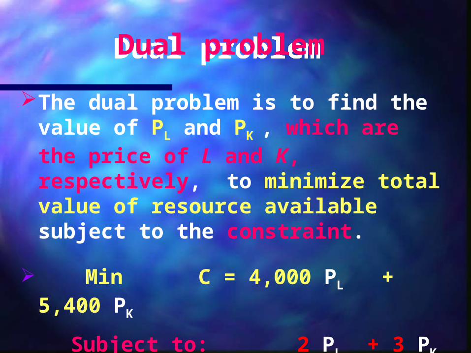
The dual problem is to find the value of PL and PK , which are the price of L and K, respectively, to minimize total value of resource available subject to the constraint.
Min C = 4,000 PL + 5,400 PK
Subject to: 2 PL + 3 PK ≧ 50 (*)
4 PL + 5 PK ≧ 80 (**)
PL ≧ 0, PK ≧ 0

Constraint (*) and (**) say that the total value of resources used in the production of a unit of output must be greater or equal to the price.
PL and PK are the prices that a manager should
be willing to pay for these resources.
They are the opportunity cost of using theses resources.
If a resource is not fully utilized, its shadow prices
will be zero, since an extra unit of the resource
would not increase total revenue (objective
function).

Max 50 Q1 + 80 Q2
S. t. 2 Q1 + 4 Q2 ≦ 4000 PL
3 Q1 + 5 Q2 ≦ 5400 PK
≦ ≦
Slack VariablesSlack Variables
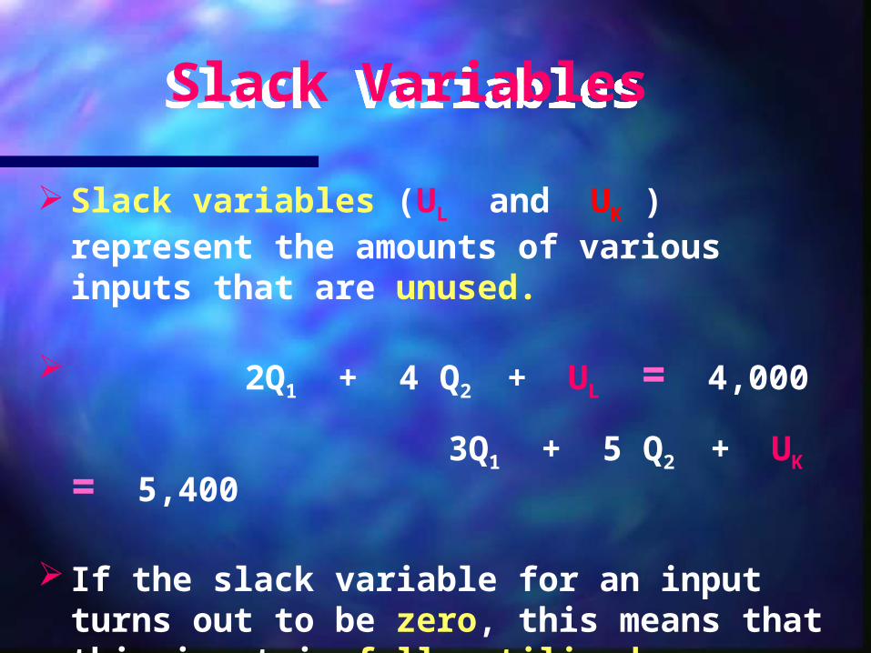
Slack variables (UL and UK ) represent the amounts of various inputs that are unused.
2Q1 + 4 Q2 + UL = 4,000 3Q1 + 5 Q2 + UK = 5,400
If the slack variable for an input turns out to be zero, this means that this input is fully utilized (Uh = 0 implies Ph > 0 , h = L, K )
If it turns out to be positive, this means that some of this input is redundant (Uh
> 0 implies Ph = 0 , h = L, K ) .

How H. J. Heinz Minimize How H. J. Heinz Minimize Its Shipping Its Shipping
How H. J. Heinz Minimize How H. J. Heinz Minimize Its Shipping Its Shipping
To determine how much ketchup each factory To determine how much ketchup each factory should send to each warehouse, Heinz has used should send to each warehouse, Heinz has used linear programming techniques. linear programming techniques.
The capacities of each factory, the requirements of The capacities of each factory, the requirements of each warehouse, and freight rates are given in the each warehouse, and freight rates are given in the first table.first table.
The optimal daily shipment from each factory to The optimal daily shipment from each factory to each warehouse is shown in the second table. For each warehouse is shown in the second table. For example, all warehouse A’s ketchup should come example, all warehouse A’s ketchup should come from factory I.from factory I.

Ware-house I II III IV V VI VII VIII IX X XI XIIA 16 16 6 13 24 13 6 31 37 34 37 40 1,820
B 20 18 8 10 22 11 8 29 33 25 35 38 1,530C 30 23 8 9 14 7 9 22 29 20 38 35 2,360D 10 15 10 8 10 15 13 19 19 15 28 34 100E 31 23 16 10 10 16 20 14 17 17 25 28 280F 24 14 19 13 13 14 18 9 14 13 29 25 730G 27 23 7 11 23 8 16 6 10 11 16 28 940H 34 25 15 4 27 15 11 9 16 17 13 16 1,130J 38 29 17 11 16 27 17 19 8 18 19 11 4,150K 42 43 21 22 16 10 21 18 24 16 17 15 3,700L 44 49 25 23 18 6 13 19 15 12 10 13 2,560M 49 40 29 21 10 15 14 21 12 29 14 20 1,710N 56 58 36 37 6 25 8 19 9 21 15 26 580P 59 57 44 33 5 21 6 10 8 33 15 18 30Q 68 54 40 38 8 24 7 19 10 23 23 23 2,840R 66 71 47 43 16 33 12 26 19 20 25 31 1,510S 72 58 50 51 20 42 22 16 15 13 20 21 970T 74 54 57 55 26 53 26 19 14 7 15 6 5,110U 71 75 57 60 30 44 30 30 41 8 23 37 3,540Y 73 72 63 56 37 49 40 31 31 10 8 25 4,410
Dailycapacity 10,000 9,000 3,000 2,700 500 1,200 700 300 500 1,200 2,000 8,900 40,000
Freight rates (cents per cwt.) from factory: Dailyrequire-ments(cwt.)

Ware-house I II III IV V VI VII VIII IX X XI XII Total
A 1,820 1,820
B 1,530 1,530C 2,360 2,360D 100 100E 280 280F 730 730G 940 940H 1,130 1,130J 4,150 4,150K 700 3,000 3,700L 1,360 1,200 2,560M 140 1,570 1,710N 580 580P 30 30Q 1,340 500 500 500 2,840R 810 700 1,510S 90 880 970T 5,110 5,110U 2,160 180 1,200 3,540Y 2,000 2,410 4,410
Total 10,000 9,000 3,000 2,700 500 1,200 700 300 500 1,200 2,000 8,900 40,000
Factory


