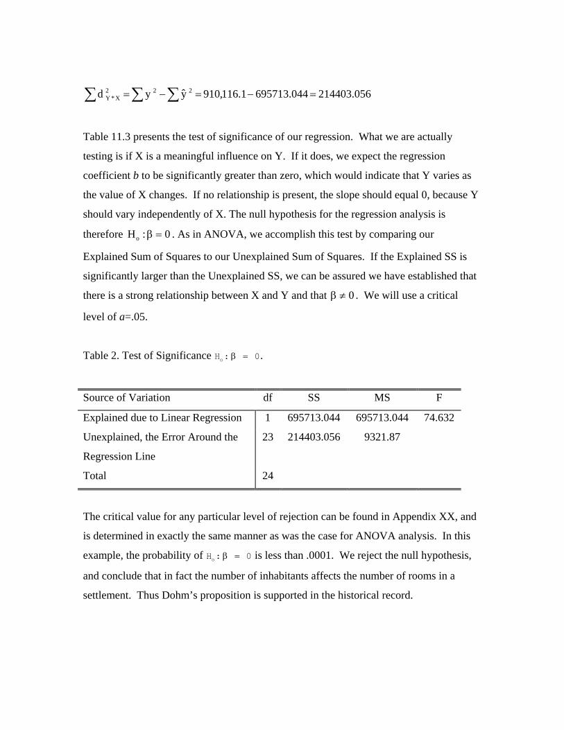
Chapter 11

Linear Regression

Linear regression is a methodology that allows us to examine the relationship between

two continuously measured variables where we believe that values of one variable may

influence the values of another. We call these functional relationships, and use

regression to:

1. Determine if there is indeed a relationship.

2. Study its shape.

3. Try to understand the nature of the relationship in terms of cause and effect.

4. Use our knowledge of the relationship to predict specific outcomes.

A functional relationship with respect to regression is a mathematical relationship that

allows us to use one variable to predict the values of another. The predictor variable is

called the independent variable, and is symbolized by the roman letter X. The predicted

variable is called the dependent variable, and is symbolized by the roman letter Y. By

independent we mean that any value of X is not determined in any way by the value of Y.

By dependent, we mean that values of Y may well be determined by values of X.

This relationship is expressed as Y=f(X).

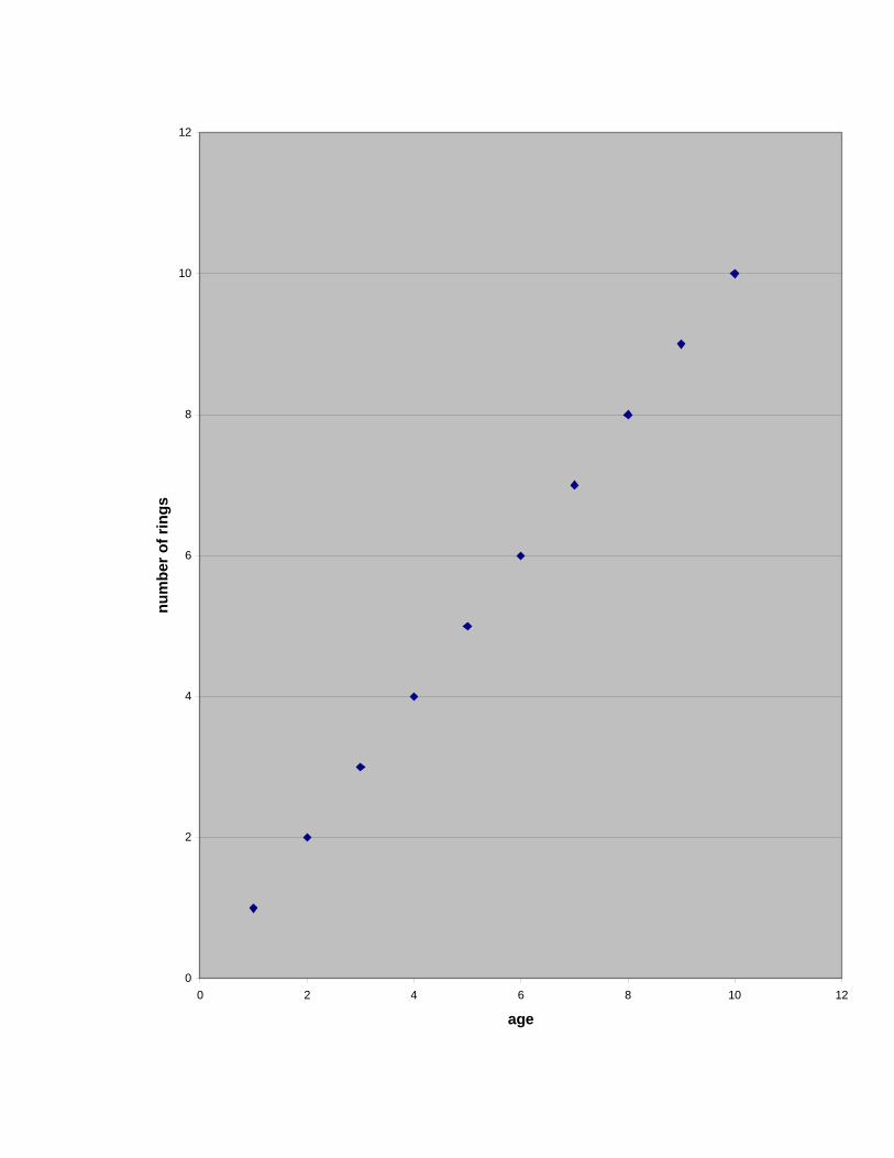
The simplest form of this expression is Y=X. An example from archaeological dating

methods can be seen in Figure 11.1, where the relationship between tree age and the

number of tree rings is presented.

Figure 11.1. The idealized relationship between age and the number of tree rings.

0

2

4

6

8

10

12

0 2 4 6 8 10

age

num

ber o

f rin

gs

12

Figure 11.1 illustrates that we can predict the number of rings on a tree once we know its

age. A more common and more complex relationship is Y=bX, where the coefficient b is

a slope factor. To illustrate this relationship, let us explore the exchange rate between the

U.S. dollar and the Mexican peso in the fall of 2003, when one dollar was equivalent to

approximately 9.5 pesos. In more formal terms, Y=9.5X. This relationship is presented

in Figure 11.2.

Figure 11.2. The relationship between the US dollar and Mexican peso in the fall of

2003.

0

10

20

30

40

50

60

70

80

90

100

0 5 10 15

U.S. Dollar

Mex

ican

Pes

o

Note that for every increase of one in the U.S. dollar, the Mexican peso increases 9.5

times.

Figures 11.1 and 11.2 illustrate functional relationships, and are used to introduce linear

regression, with regression symbols, X and Y. Yet, it is important to note that in both of

these examples causality is not implied. Age doesn’t cause tree rings, and change in the

U.S. dollar does not directly cause the Mexican peso to change. In these situations the

symbols X and Y are used for the sake of illustration.

We do, however, recognize that there is a relationship between age and the number of

tree rings and between the values of the U.S. dollar and the Mexican peso, as our

economies are very much interdependent. Interdependence of variables is the subject of

the next chapter, correlation.

Regression is used when there is a reason to believe (to hypothesize) that there is a

relationship such that the variable represented by X actually causes the value associated

with Y to change. Let us consider a non-archaeological example to illustrate this case.

Figure 11.3 illustrates the relationship between age and diastoloic blood pressure in

humans. Given our knowledge of human physiology and the effects of aging, we might

very well expect for there to be some relationship between age and blood pressure such

that an individual’s age actually affects his or her blood pressure. This hypothesis

appears to be supported in Figure 11.3, in which the average blood pressure increases

according to the individuals’ ages.

Figure 11.3. Average diabolic blood pressure of humans of various ages.

0102030405060708090

0 10 20

Age

Blo

od P

ress

ure

30

While increases in X and Y in Figures 11.1 and 11.2 were uniform, notice that this is not

the case in Figure 11.3. Notice also that Y=0 when X=0 in those figures, but that this is

not the case here. Figure 11.4 illustrates that if we draw a line through the data points

toward the Y axis, we can estimate where that line intercepts that axis.

Figure 11.4. Regression line describing the relationship between age and diastolic blood

pressure.

0

10

20

30

40

50

60

70

80

90

5 7 9 11 13 15 17 19 21

Age

Blo

od P

ress

ure

It appears that the line would intercept the Y axis near 60. This makes sense; newborns

have blood pressure.

As you can see, the line has both an intercept (the point at which it crosses the Y axis)

and a slope (the rate at which Y changes in accordance with changes in X). For any

given relationship we can have a potentially infinite number of intercepts and slopes.

These relationships take the general form Y=a+bX. This is called the general linear

regression equation, where a is the intercept, and b is called the regression coefficient or

slope. Using our knowledge of age (X), the intercept, and the regression coefficient, we

can predict a value of Y for any value of X provided in the data above.

In most applications, as in Figure 11.4, data points are scattered about the regression line

as a function of other sources of variation and measurement error. The functional

relationship between X and Y does not mean that given an X, the value of Y must be

a+bX, but rather that the mean of Y for a given value of X is at a+bX.

There are four assumptions of simple linear regression.

1. X is measured without error, or, in fancy statistical terms, it is fixed. While Y may

vary at random with respect to the investigator, X is under the investigator’s control.

This simply means that we specify which X or X’s we are interested in examining.

2. The expected value for the variable Y is described by the linear function:

. Put another way, the parametric means of Y are a function of X and

lie on a straight line described by the equation.

XY β+α=µ

3. For any given value Xi, the Y’s are independent of each other and normally

distributed. This means that the value of one particular Y doesn’t influence the

values of other Ys, and that they are normally distributed. The formula for a given Y

is therefore , where iii XY ε+β+α= iε is an error term reflecting variation caused

by factors other than X.

4. The samples along the regression line are homoscedastic—they have similar

variances. Variances of similar magnitude are essential for useful prediction.

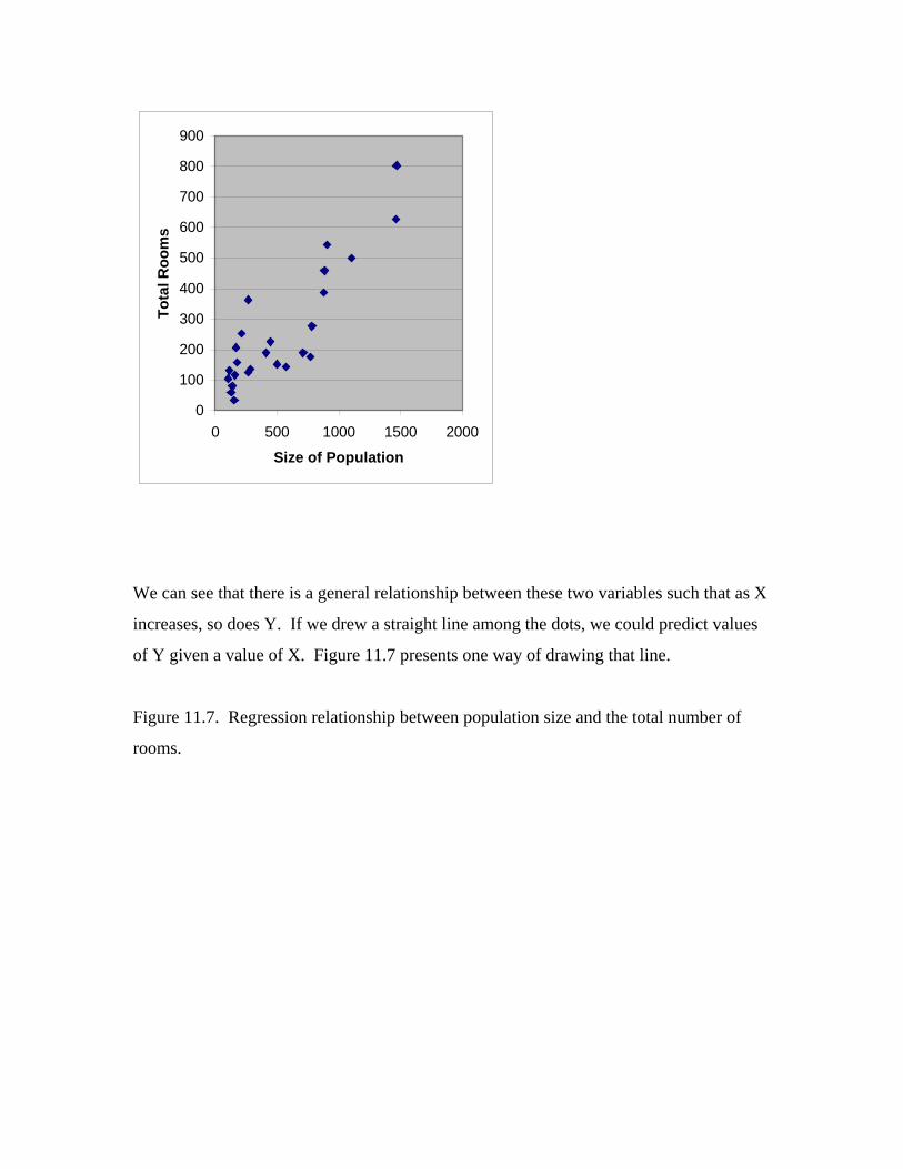
Here, recall that the purposes of regression are to determine if there is a relationship,

study the shape of it, try to understand the relations of cause and effect, and predict Y

with knowledge of X. These four assumptions make this possible.

The Construction of theRegression Equation

With the basic regression formula in its most simple form, Y=a+bX, we must first

determine a and b to solve for Y for a given X. To illustrate how this is accomplished, let

us continue with our our blood pressure example. For our calculations, we first need to

know that X =13 and Y =72.44. We also need the information presented in Table 11.1.

Table 11.1. Summary information for the relationship between age and diastolic blood

pressure.

Step # 1 2 3 4 5 6 7 8 9 10

Age Blood

Pressure

x Y Sum of

Products

2X*Yd

(Deviation

of Y at X)

Unexplained

Sum of

Squares

y Explained

Sums of

Squares

X Y )XX( i −

)YY( i −

2x xy 2y Y )YY( − 2

X*Yd )YY( −

2y

1 5 60 -8 -12.44 64 99.56 154.8

6

62.37 -2.37 5.62 -10.07 101.49

2 7 63 -6 -9.44 36 56.67 89.20 64.89 -1.89 3.57 -7.55 57.07

3 9 69 -4 -3.44 16 13.78 11.86 67.41 1.59 2.53 -5.03 25.35

4 11 74 -2 1.56 4 -3.11 2.42 69.92 4.08 16.65 -2.52 6.37

5 13 75 0 2.56 0 0.00 6.53 72.44 2.56 6.55 -0.00 0.00

6 15 71 2 -1.44 4 -2.89 2.09 74.96 -3.96 15.68 2.52 6.33

7 17 77 4 4.56 16 18.22 20.75 77.47 -0.47 0.22 5.03 25.26

8 19 85 6 12.56 36 75.33 157.6

4

79.99 5.01 25.10 7.55 56.94

9 21 78 8 5.56 64 44.44 30.86 82.51 -4.51 20.34 10.07 101.32

Sum 117 652 0 0 240 302 476.2

2

651.96 0.04 96.26 0 380.12

As part of solving for a and b and building our regression equation, we are also

explaining how much variation in Y is explainable in terms of X. The portion of the

variation in Y that cannot be explained by X is unexplainable in terms of X and is the

result of the influence of other variables or measurement error. While building our

regression equation, we also build an explained sum of squares, which describes the

portion of the variation in Y caused by X, and an unexplained sum of squares, which

describes all other sources of variation. To do so, we proceed in the following manner

illustrated on Table 11.1:

Column 1 presents x, the deviation of each X from its mean. Notice that this sums to

zero.

Column 2 presents y, the deviation of each Y from its mean. This too sums to zero.

Column 3 presents our x's squared, the sum of which is used in the denominator of the

calculation of b, or our regression coefficient, in the formula: . ∑ ∑= 2x/xyb

Column 4 presents the sum of products, that is, the product of x and y. The sum of these

products is used in the numerator of our calculation of b where . ∑ ∑= 2x/xyb

Column 5 presents our ys squared, which is the total sum of squares.

Column 6 presents our predicted value of Y for a given X, and is vocalized as Y-hat. To

calculate this value we proceed in the following manner. We first calculate the

regression coefficient (or slope):

∑ ∑= 2x/xyb

b = 302/240

b = 1.2583

Now that we have our slope, we can plug it into the regression equation and solve

for a, for a given value of Y. Our regression equation is: Y=a+bX. With least

squares regression, the predicted line of values always passes through the mean of

both X and Y. Therefore, we can subsitute those values and solve for a.

XbaY +=

XbYa −=

a = 72.44 - (1.2583*13)

a = 56.0821

Given:

bXaY += ,

then =56.0821 + 1.2583(X). Y

We may then solve for every value in Column 6.

Column 7 presents the deviations of Y at X from ,our expected value of Y. This is the

variation from the point on the line for each X illustrated in Figure 11.4 and the

actual value of Y.

Y

Column 8 is Column 7 squared, or the unexplained sum of squares.

Column 9 presents the deviations of the predicted Y's from their mean. Figure 11.5

displays this deviation graphically.

Column 10 presents Column 9 squared, or the explained sum of squares. Notice that

Column 10 the explained sum of squares, and Column 8, the unexplained sum of

squares sum to Column 5, the total sum of squares.

Figure 11.5. Illustration of the explained and unexplained variation.

wpe1.gif (4334 bytes)

To understand regression, it is critical to understand the relationships presented in Figure

11.5. An individual observation varies from the mean of Y. This deviation is 11 Y,X

)YY( − , and is symbolized by y. These are the deviations represented by the Total Sum

of Squares. Some of this deviation can be explained in terms X. That is, we can explain

the deviation of our predicted Y from the mean of Y, or )YY( − . This is symbolized

by . This allows us to calculate the Explained Sum of Squares. That leaves us with the

deviation , symbolized by , which we cannot explain. This is called the

Unexplained Sum of Squares. By unexplained, we mean unexplained in terms of X. It

may be variation that can be explained in terms of an additional variable(s) or as the

product of measurement error.

y

)YY( − X*Yd

We now have the regression equation , so we can now predict Y

for a given X. But how do we determine if the relationship itself is significant? In other

words, how do we tell if there is actually a relationship between X and Y such that a

significant portion of the variation in Y is attributable to the variation in X? We take this

up in the following section.

)X(2583.10821.56Y +=

Computational Procedures for Regression

To illustrate the usefulness of regression and how one can evaluate the strength of a

relationship between a dependent and independent variable, let us consider an

archaeological example presented by Karen Dohm. Archaeologists are often interested in

recontructing the number of individuals who once occupied a settlement that today is an

archaeological site. As a researcher intererested in the prehistory of the American

Southwest, Dohm proposed that the number of rooms in a settlement should be a function

of the number of people living there. Expressed more formally, we can write this as a

functional relationship in the form Y=f(X), or the number of rooms in a settlement = f

(the number of people in a settlement).

Dohm’s premise seems intuitively reasonable; more people will need more storage and

habitatation rooms, all other variables being equal. The only problem is that we have no

information on X, the number of people in a settlement today represented by an

archaeological site. As a solution to this problem Dohm gathered information on historic

groups who are likely descended from the people who built the prehistoric settlements,

and who today live in similar buildings. These data are presented in Table 11.2. With

this information, she hoped to provide a means of estimating population sized for

archaeological sites. She first had to demonstrate that a relationship between population

size and the number of rooms in a settlement was in fact present. This is a regression

problem that is graphically illustrated in Figure 11.6.

Table 11.2. Historic Pueblo Room Count Analysis (Dohm).

Pueblo Map

Date

Pop. Total

Rooms

Room-

blocks

# Rooms in

Room Block

Ave Number

Contiguous

Rooms

Rooms per

Family

Rooms per

Person

Acoma 1948 879 387 11 360 13.3 1.792 0.440

Cochiti 1952 444 225 11 98 4.1 1.940 0.507

Isleta 1948 1470 804 42 546 5.3 2.300 0.547

Jemez 1948 883 459 22 274 5.7 2.782 0.520

Laguna 1948 711 189 14 114 6.1 1.432 0.266

Nambe 1948 155 34 2 15 3.4 1.000 0.219

Picuris 1948 130 59 2 16 2.5 2.185 0.454

San Felipe 1948 784 276 11 180 4.2 1.653 0.352

San Ildefonso 1948 170 207 6 107 4.7 6.469 1.218

San Ildefonso 1973 413 189 11 120 4.3 - 0.458

San Juan 1948 768 176 12 159 8.8 1.143 0.229

Sandia 1948 139 80 4 36 3.2 2.105 0.576

Santa Ana 1948 288 136 9 102 5.4 1.838 0.472

Santa Ana 1975 498 152 10 82 3.7 - 0.305

Santa Clara 1948 573 144 6 111 6.9 1.180 0.251

Santo Domingo 1948 1106 500 26 377 6.0 2.392 0.452

Shipaulovi 1882 113 131 1 129 65.5 5.955 1.159

Shongopavi 1882 216 253 5 248 36.1 - 1.171

Sichomovi 1882 104 105 3 96 17.5 4.375 1.010

Taos 1948 907 543 14 495 14.7 2.598 0.599

Taos 1973 1463 627 21 480 6.3 2.083 0.429

Tesuque 1948 160 116 3 88 7.3 4.462 0.725

Tewa Village 1882 175 158 4 157 26.3 4.514 0.903

Walpi 1882 270 363 5 356 45.4 6.368 1.344

Zia 1948 267 126 8 89 4.5 2.571 0.472

Figure 11.6. The relationship between site population and the total number of rooms.

0

100

200

300

400

500

600

700

800

900

0 500 1000 1500 2000

Size of Population

Tota

l Roo

ms

We can see that there is a general relationship between these two variables such that as X

increases, so does Y. If we drew a straight line among the dots, we could predict values

of Y given a value of X. Figure 11.7 presents one way of drawing that line.

Figure 11.7. Regression relationship between population size and the total number of

rooms.

0

100

200

300

400

500

600

700

800

900

0 500 1000 1500 2000

Population

Num

ber o

f Roo

ms

The line if Figure 11.7 is calculated by solving for a and b as previously illustrated, and

is called the least squares regression line. As expected, we can see in Figure 11.7 that

each observation deviates from the regression line in greater or lesser degrees. We also

know that each value for X and Y differs from their respective means in greater or lesser

degrees as well. These deviations allow us to compute explained and unexplained sums

of squares, which can be compared with each other in a manner conceptually identical to

the sum of squares calculated in ANOVA. To do this, let us follow the following

procedure:

Compute sample size, sums, sums of the squared observations, and the sum of the Xys.

n=25

∑ = 086,13X

∑ = 439,6Y

∑ = 270,996,10X2

∑ = 545,568,2Y2

∑ = 899,068,5XY

The means, sums of squares, and the sums of products are calculated as previously

illustrated and are:

44.523X =

56.257Y =

∑ = 532,146,4x 2

∑ = 1.166,910y2

∑ ∑ ∑ ∑−=n

)Y)(X(XYxy

25

)439,6)(086,13(5068899−=

84.468,698,1=

The Regression Coefficient is:

4096. 4146532

84.1698468 xxy

b 2X*Y ===∑∑

The Y intercept is:

)44.523( 4096. 56.257 )X(bYa X * Y −=−= = 43.1527

The Explained Sums of Squares is:

∑ ∑∑ === 044.695713

4146532)84.468,698,1(

x)xy(

y2

2

22

The Unexplained Sum of Squares is:

∑ ∑ ∑ =−=−= 056.214403 044.6957131.116,910 yy d 2 2 2 X * Y

Table 11.3 presents the test of significance of our regression. What we are actually

testing is if X is a meaningful influence on Y. If it does, we expect the regression

coefficient b to be significantly greater than zero, which would indicate that Y varies as

the value of X changes. If no relationship is present, the slope should equal 0, because Y

should vary independently of X. The null hypothesis for the regression analysis is

therefore . As in ANOVA, we accomplish this test by comparing our

Explained Sum of Squares to our Unexplained Sum of Squares. If the Explained SS is

significantly larger than the Unexplained SS, we can be assured we have established that

there is a strong relationship between X and Y and that

0:Ho =β

0≠β . We will use a critical

level of a=.05.

Table 2. Test of Significance Ho: β = 0.

Source of Variation df SS MS F

Explained due to Linear Regression 1 695713.044 695713.044 74.632

Unexplained, the Error Around the

Regression Line

23 214403.056 9321.87

Total 24

The critical value for any particular level of rejection can be found in Appendix XX, and

is determined in exactly the same manner as was the case for ANOVA analysis. In this

example, the probability of Ho: β = 0 is less than .0001. We reject the null hypothesis,

and conclude that in fact the number of inhabitants affects the number of rooms in a

settlement. Thus Dohm’s proposition is supported in the historical record.

Another way to present the significance of the result is to present the explained SS as a

proportion of the total SS. The value is called the regression coefficient and is

represented by the symbol of 2r . In this case:

7644.100.910116044.695713

TotalSSSExplainedSr 2 ===

These values range from zero to one. The higher the ratio, the higher proportion of the

variation in Y that is explained by X. It is possible to have a significant relationship, in

which , but to have very little of the actual variation in Y explainable by X. This

type of relationship is indicated by a significant F value for the ANOVA, but a low

0≠β

2r

value. In such cases, other variables likely significantly influence the value of Y, perhaps

indicating that we should rethink the variables used in our analysis and prompting us to

consider the influence of additional variables. In terms of the formal presentation of the

results, present both the regression equation and the r squared value.

The Analysis of Residuals

The analyst needs to take one additional precaution to determine if a linear model is

appropriate. This step is an analysis of the deviations of our actual observations (Y) from

our predicted Y ( ), which ultimately were used to calculate our unexplained sum of

squares. Residuals for our pueblo room example are presented in Table 11.3.

Y

Table 11.3. Residuals calculated as Y - . Y

Observation Predicted Y Residuals 1 403.2016 -16.2016 2 225.0204 -0.02043 3 645.2822 158.7178 4 404.8400 54.15995 5 334.3868 -145.3870 6 106.6426 -72.6426 7 96.4023 -37.4023 8 364.2885 -88.2885 9 112.7868 94.21322 10 212.3225 -23.3225 11 357.7347 -181.735 12 100.0888 -20.0888 13 161.1210 -25.1210 14 247.1395 -95.1395 15 277.8604 -133.8600 16 496.1835 3.816502 17 89.4389 41.5611 18 131.6289 121.3711 19 85.75239 19.24761 20 414.6707 128.3293 21 642.4149 -15.4149 22 108.6907 7.309342 23 114.8348 43.16516 24 153.748 209.252 25 152.5191 -26.5191

Figure 11.8 presents a plot of these residuals. The examination of residuals allows for

the judgement of whether or not a linear model is appropriate. A perfect fit would be

illustrated by a random distribution of residual points about the value of 0, such as that

illustrated in Figure 11.8. A "run" of individuals on one side of the line, say if all of the

residuals illustrate in Figure 11.8 for s greater than 500 were above the line while

residuals for s less than 500 were below the line, would indicate that the assumption of

the linear model is not met. A run of points on one side of the line, followed by a run of

iY

iY

points on the other side of the line, followed by a return to the other side, would indicate

that a curvilinear model is likely more appropriate. Increasing distance from 0 with

larger values would likely indicate unequal variances, or heteroscedasticity, a violation of

the assumptions of regression.

wpe5.gif (7842 bytes)

Significance Tests and Confidence Limits for Regression

At times we wish to test a variety of hypotheses with regression analysis. Most often

these are accomplished through the construction of confidence limits. The following

section introduces several of the more common calculations and tests.

Standard Error of the Regression Coefficent. This standard error is needed whenever one

wishes to put confidence limits around regression coefficient, or slope. For example, we

might wish to compare two or more slopes to determine if they are significantly different

or not. We might wish to compare the slope describing the relationship between

population size and the number of rooms among Puebloan groups with that of

Mesoamerican groups to see if the relationships between population size and settlement

size are the same, or if behavioral differences result in differences in settlement size.

0474.4146532

87.9321x

Ss 2

2 X * Y

b ===∑

Once we have the standard error of the regression coefficient, we can built confidence

limits as follows:

0981. )0474. (069.2 Sb t ] 23 [ 05. ==

3115. 0981. 4096. Sb tb L ] 23 [ 05. 1 =−=−=

5077. 0981. 4096. Sb tb L ] 23 [ 05. 2 =+=+=

Testing Significance of the Regression Coefficient. We tested the significance of the

regression coefficient above by using the F distribution. Another way of testing for the

significance of the regression coefficient is to use the t-distribution as follows.

6413.8 0474.4096.

S0b t

b

Y*Xs ==

−=

069.2 t ] 23 [ 05. =

767.3 t ] 23 [ 001. =

Since 8.6413 is larger than either value, p<.001.

Confidence Limits around for a Given X. We can also place confidence limits

around any section of our regression line. This is helpful in cases in which we wish to

know the potential range that likely includes our population parameters . After all a

regression line isn’t particularly helpful if we don’t know how close the values

iYµ

iYµ

represented by the line are to the values were are really trying to estimate, i.e., the mean

of Y at each . Our conclusions might be very different if we expect a wide range of

potential variation instead of a very narrow range.

iX

We could simply calculate confidence intervals using the standard error of the sample at

each as described in the chapter discussing the t-test, but such an approach doesn’t

take advantage of the total amount of information available from the regression analysis.

Using regression, we can make more accurate predictions of

iX

iYµ than is possible

otherwise (assuming that there is a strong relationship between X and Y). As a result,

our confidence intervals around will be smaller than those derived by considering the

variation in Y and a particular independently. Thus, knowledge about the

relationship between X and Y allows us to better predict

Y

iX

iYµ than would be possible

otherwise.

Confidence limits are most easily calculated around the sample mean of Y at X , which,

as previously mentioned, is the anchor point through which the least squares regression

line must pass. In this case, the standard error of Y is calculated as:

3099.19 25

87.9321 n

S S2

X * Y Y ===

95% confidence limits for the mean Yµ corresponding to X ( 56.257Y = ) are

determined as:

9523.39 )3099.19( 069.2 t ] 23 [ 05. ==

6077.217 9523.3956.257 S tY L Y ] 23 [ 05. 1 =−=−=

5123.297 9523.3956.257 S tY L Y ] 23 [ 05. 2 =+=+=

Calculating confidence intervals around any given is more difficult though, because of

the uncertainty associated with our estimate of the regression coefficient. Because of the

structure of the regression line, it must pass through

Y

Y at X , allowing the confidence

limits around this point to be quite tight. As one moves away from this point towards

either end of the regression line, the variation in b results in an increasingly large

confidence limits; even a slight difference in b can result in very different s over a long

distance. As a result, our estimate of becomes increasingly less accurate the farther we

move from

Y

Y

Y at X . The calculation of the confidence intervals must consequently

account for this.

The standard error of for a given value of is calculated as follows: Y iX

⎥⎦

⎤⎢⎣

⎡∑−

+= X

)XX(n1 S S 2

2 i 2

X * Y y

Notice that this value will increase exponentially as the distance between and iX X

increases.

Continuing with Dohm’s example, for 1250Xi = :

4921.39 4146532

)44.5231250(251 87.9321 S

2

y =⎥⎦

⎤⎢⎣

⎡ −+=

95% confidence limits for corresponding to the estimate at

are calculated as:

i Y µ bXaYi += 1250X i =

bXaYi +=

)1250(4096.1527.43Yi +=

152.555Yi =

7091.81 )4921.39( 069.2 S t Y ] 23 [ 05. ==

4428.473 7091.81152.555 S tY L Y ] 23 [ 05. 1 =−=−=

8611.636 7091.81152.555 S tY L Y ] 23 [ 05. i 2 =+=−= .

Standard error of a predicted mean i Y in a new sample of . Sometimes we might

wish to compare a newly determined

iX

i Y to our to determine if it is significantly

different than the value expected from the regression analysis. This is particularly helpful

when we believe behavioral or depositional factors might cause differences in the

archaeological record. For example, perhaps we suspect the relationship between

population size and the number of rooms is different for agricultural field houses or for

ceremonially significant sites than is the case in generalized habitations.

Y

When we wish to compate a new i Y to , the best predictor of the mean is Y .

Using Dohm’s example for , = 555.152. We must also take into account

the sample size used to determine the new

YiYµ ˆ

1250X i = Y

i Y . If the new sample was based on a sample

size of K = 5, the standard error of the predicted mean is:

⎥⎦

⎤⎢⎣

⎡∑−

++= X

)XX(n1

K1 S S 2

2 i 2

X * Y Y

⎥⎦

⎤⎢⎣

⎡++=

4146532) 44.253 * 1250 (

251

51 87.9321 S

2

Y

51.58 S Y =

95% prediction limits for a sample mean of 5 settlements at 1250 people can then be

calculated as:

0675.121 )51.58( 069.2 S t Y ] 23 [ 05. ==

087.434 065.121152.555 S t Y L Y ] 23 [ 05. i 1 =−=−=

217.676 065.121152.555 S tY L Y ] 23 [ 05. i 2 =+=+= .

These are the basics of regression. When we wish to examine the nature of a relationship

between two continuously measured variables where an argument of cause cannot be

made, we turn to correlation, the subject of the next chapter.