Linear stability of free shear flow of viscoelastic liquids · 2009-07-21 · Linear stability of...

http://journals.cambridge.org Downloaded: 21 Jul 2009 IP address: 131.111.16.227

J . Fluid Mech. (1994), 001. 268, pp. 31-69 Copyright Q 1994 Cambridge University Press

37

Linear stability of free shear flow of viscoelastic liquidst

By J. AZAIEZ A N D G. M. HOMSY Department of Chemical Engineering, Stanford University, Stanford, CA 94305-5025, USA

(Received 3 June 1992 and in revised form 8 November 1993)

The effects of viscoelasticity on the hydrodynamic stability of plane free shear flow are investigated through a linear stability analysis. Three different rheological models have been examined : the Oldroyd-B, corotational Jeffreys, and Giesekus models. We are especially interested in possible effects of viscoelasticity on the inviscid modes associated with inflexional velocity profiles. In the inviscid limit, it is found that for viscoelasticity to affect the instability of a flow described by the Oldroyd-B model, the Weissenberg number, We, has to go to infinity in such a way that its ratio to the Reynolds number, G K We/Re, is finite. In this special limit we derive a modified Rayleigh equation, the solution of which shows that viscoelasticity reduces the instability of the flow but does not suppress it. The classical Orr-Sommerfeld analysis has been extended to both the Giesekus and corotational Jeffreys models. The latter model showed little variation from the Newtonian case over a wide range of Re, while the former one may have a stabilizing effect depending on the product sWe where s is the mobility factor appearing in the Giesekus model. We discuss the mechanisms responsible for reducing the instability of the flow and present some qualitative comparisons with experimental results reported by Hibberd et al. (1982), Scharf (1985a, b) and Riediger (1989).

1. Introduction Developing an understanding of instability and transition in free shear flows at high

Reynolds numbers has been a central problem in the theory of fluid motion for over a century. In the present study we are concerned with the instability of viscoelastic fluids in free shear flow and in particular in the possibility that viscoelasticity may significantly affect the inviscid modes associated with inflexional velocity profiles. Thus, our work is distinguished from that of most previous investigators who focused on the Newtonian mixing layer. The last decade has seen important progress in the understanding of the mechanisms governing the process of transition to turbulence in free shear layers (see e.g. Ho & Huerre 1984; Corcos & Lin 1984; Herbert 1988; Metcalfe et al. 1987; Moser & Rogers 1991). Important understanding of the mechanisms of vorticity production, subharmonic (pairing) instabilities, and vortex stretching has come from such studies. This understanding opens the possibility of rational methods of manipulation and active control of turbulence by influencing transition mechanisms. Examples of such manipulation include the use of time- dependent motion of boundaries, modification of the properties of surfaces, including grooves and ribs, and addition of polymers and/or fibres to the flow. It is this last

t With Appendix E by E. J. Hinch.

http://journals.cambridge.org


38 J. Azaiez and G. M . Hornsy

method that is relevant to the present study. It has been known for over forty years that the addition of small amounts of dissolved polymer can dramatically reduce turbulent drag. There is in fact a large literature on the subject: see for example the review by Berman (1978). In itself this paper is not directly relevant to drag reduction but is a first step in the study of high-Reynolds-number non-Newtonian flows with shear.

There are only a few experimental studies of viscoelastic free shear flows and there is little understanding of how polymers affect either primary or secondary instability modes. Recently Hibberd, Kwarde & Scharf (1982), Scharf (1985a, b) and Riediger (1989) studied the effects of the addition of polymers and surfactants on the instability of the mixing layer. The results of the experimental measurements and flow visualizations show a delay in the formation of the typical structures of the plane mixing layer, i.e. roll-up and pairing. They also reveal that the presence of polymer additives leads to an enhancement of the large-scale turbulent structures and an almost complete suppression of the small-scale structures.

The motivation for the present linear stability analysis is two-fold: first we want to determine the effects of the addition of polymers on the instability of inviscid plane shear flows, and second we wish to establish the conditions under which viscoelasticity affects the flow and understand the mechanisms involved.

We comment that unlike the Newtonian case, predictions are likely to depend upon details of the equations relating stress to shear rate. The relation between these two tensors is nonlinear and usually involves an integral or differential equation known as the constitutive equation. For a thorough discussion of the development of rheological constitutive equations for viscoelastic fluids and their application in fluid dynamics see Goddard (1979), Bird et al. (1987) and Larson (1988). In the present study, we will examine three rheological models. Initially we use the Oldroyd-B model and establish that, for this model, there is a reduction of the instability modes due to a coupling between the vorticity and the normal stresses. This coupling is characterized by a dimensionless number, G, that involves only fluid properties and is independent of kinematics. In addition we will present the results of an asymptotic analysis in the limit of large G . Finally, we give predictions of the effects of viscoelasticity on the mechanisms usually observed in the Newtonian mixing layer.

This stabilizing effect raised questions about the robustness of the mechanisms of stabilization to details of the rheological model. In fact since the Oldroyd-B model has no shear thinning or plateau of normal stress, its range of applicability is limited to dilute solutions and to moderate shear rates (Bird et al. 1987). Thus, is we wish to describe more general viscoelastic behaviour, we must have a rheological equation of greater generality that can achieve a closer correspondence with the known rheological properties. For this purpose we examined two models known to describe qualitatively many observed rheological effects of non-Newtonian fluids : the corotational Jeffreys model and the Giesekus model. For these models, we found no effect on the inviscid modes as Re +a. Accordingly, the classical Orr -Sommerfeld analysis has been extended to both of these models, and we studied the effects of viscoelasticity at finite Reynolds number.

2. Problem definition The mixing-layer flow configuration is standard, as shown in figure 1 . U, (respectively

U,) is the free-stream velocity of the upper (lower) flow. We denote by uo = i(U, - U,) the free-stream velocity in a reference frame moving with the average velocity of the flow +(q + &), and by S the momentum thickness of the mixing layer. In all the



Stability of free shear flow of viscoelastic liquids 39

i -0

FIGURE 1. Schematic of the mixing layer.

subsequent analysis, we use uo as the reference velocity and 6 as the reference length to make our equations dimensionless. The flow is governed by the continuity and Cauchy momentum equations :

v*v = 0, (1)

DV P- Dt = -vp+v ‘7;

v is the velocity vector, p the dcnsity, p the isotropic prcssure and T the extra stress tensor. In dimensionless form, ( 1 ) and (2) are characterized by one dimensionless group, the Reynolds number, Re = ~ S U , / T , I , where T,I is a measure of the shear viscosity of the fluid. Equations (1) and (2) are closed through evolution equations for the extra stress tensor T. We use a class of differential models of the form h D.c/Dt =AT, u, Vv), the details of which will be given in the next section. Scaling of this class results in at least one additional parameter, the Weissenberg number, We = hu,/S, a dimensionless measure of the polymer relaxation time, A.

We make the standard parallel-flow assumption and take the mean flow as

v,(Y> = tanh(y),

wo(y) = tanh(y)2- 1, UI,(y) = log(cosh(y)). (3)

Here U,(y) is the streamwise velocity, wo(y) the spanwise vorticity and uI,(y) the associated streamfunction expressed in dimensionless form. Note that (3) is a solution of the Cauchy equation provided that there is a dimensionless body force

where uy2 is the shear component of the base state polymer stress a. The expression for a& depends on the specific rheological model, but as we will see in the next section, it is O(1) uniformly in the flow domain. As a consequence, we can argue that the correction due to F is uniformly U ( l / R e ) in space for all three rheological models.

We assume that the laminar flow is quasi-parallel, i.e. that its variation is entirely in the direction normal to the flow, and that the disturbances are wave-like. The parallel-



40 J . Azaiez and G. M . Homsy

flow assumption is a satisfactory first approximation for treating the linear stability of viscous flows at sufficiently high Re (see Ling & Reynolds 1973). In Appendix A, we analyse the correction to the laminar flow of a Newtonian fluid due to the presence of viscoelasticity for the Oldroyd-B model in the special inviscid limit, Re < 1, We < 1 and We/Re = O(1). In this analysis we show that the expansion leads to an equivalent Blasius problem and that, using a simple transformation, the base-state flow profile can be mapped into the Blasius profile. Since solutions for the mixing layer are known to be closely approximated by the profile given in (3), we conclude that this profile is also satisfactory for the purpose of examining inviscid modes of the viscoelastic mixing layer described by the Oldroyd-B model. For other models, we expect that the quasi- parallel-flow assumption will be still valid at finite Reynolds numbers.

For the parallel flow of a Newtonian fluid, the theorem of Squire (1933) states that two-dimensional disturbances are temporally more unstable than three-dimensional disturbances, and an investigation of two-dimensional disturbances is sufficient to determine the critical Reynolds number. The equivalent Squire theorem for the flow of a viscoelastic fluid described by any of the three rheological models examined in this study has not been proved or disproved in the viscous case. In the special limit of the inviscid highly elastic mixing layer described by the Oldroyd-B model, we show that there is a Squire's transformation (see Appendix B) showing that linear theory does not distinguish between two- and three-dimensional modes in the special limit Re +a, G - We/Re = O(1).

In the present study we will consider only the case of purely two-dimensional disturbances even though we are aware that viscoelasticity may introduce a new type of instability which, if associated with a wave growing in the spanwise direction, will lead to a competition between elastic instabilities and those associated with viscous mechanisms (Giesekus 1966).

3. Linear stability analysis We study the linear stability of (3) and its associated stress field. For any constitutive

equation the streamfunction and the stress components are represented by the base- state profile plus a small perturbation. The expressions are substituted into the equations which are linearized in the usual way. Perturbations quantities are then Fourier transformed in x and t :

Y ( y ) = Y'&) + $ ( ~ ) e ~ ~ ( ~ - ' ~ ) , ~ ( y ) = T&) + T(y)eia(s-ct), etc. (4)

We treat the temporal stability of the flow, so a is the real wavenumber and c is the complex frequency.

In the subsequent analysis, the extra stress tensor T is written as the sum of two stresses (Larson 1988) :

T = T S + T P (5) The first term corresponds to the contribution of the Newtonian solvent and is proportional to the shear rate tensor y = ( V V ) + ( V V ) ~ :

TS = ys+, (6) with q8 the solvent viscosity. The second term represents the polymeric contribution, which we write as

where yp is the polymeric contribution to the shear viscosity. We let K = y8/(ys + rp) =

r p a, (7) +J =



Stability of free shear f low of viscoelastic liquids 41

ys/q and throughout this study y = qs+vp denotes the total viscosity of the fluid. Equation ( 5 ) then becomes

Using these expressions, the perturbation vorticity equation is

7 = $ K Y + ( 1 - K ) a ] . (8)

We see that elasticity can have an effect on the inviscid mode for Re-tco only if the elastic stress components are large. Substituting the expressions in (4), we obtain the following linearized Cauchy equation in terms of the streamfunction 4 :

K ia{(V,-c)(D2-a2)-D2~}--(D2-a2)2 $ = ~ [ ( [ ( D 2 + a 2 ) a 1 2 + i a D ( a l l - ~ 2 2 ) ] ,

Re I Re (10)

where D = d/dy. In the following subsections we give the differential equations satisfied by the tensor a for the three rheological models that we are examining and present the linearized equations that govern disturbances to the steady base flow.

[

3.1. The Oldroyd-B model The Oldroyd-B model describes well the behaviour of polymeric liquids composed of a low concentration of high-molecular-weight polymer in a very viscous Newtonian solvent at moderate shear rates. These fluids have come to be known as Boger fluids. Data on well-characterized Boger fluids are available (Boger 1977; Mackay & Boger I987), allowing a comparison of theoretical predictions with experimental results. The Oldroyd-B rheological equations can be derived from a molecular model in which the polymer molecule is idealized as a Hookean spring connecting two Brownian beads (Bird et al. 1987).

The tensor a satisfies the upper convected Maxwell equation

v ha+a = y ,

is the upper-convected derivative of a, and h is the polymer relaxation time. The Oldroyd-B model contains both the upper-convected Maxwell fluid (ys = 0-

K = 0) and the Newtonian fluid ( y p = 0 o K = 1). This model gives a reasonably good qualitative description of dilute polymer solutions. It predicts no shear thinning, and a constant first normal stress coefficient, !PI = 2hyp. It also predicts a zero second normal stress coefficient Y,.

The expression for the base-state tensor a is

ayl(y) = 2Wew& ay,(y) = -wo, at,(y) = 0. (13)

Expressing all the variables in terms of the streamfunction disturbance $ and arranging the expressions, we obtain the following equation :

(14) 1 - K 1 SRe ,=’

K ia{(U, - c) (D2 - 2) - D 2 q ) --(D2 - a2)2 q5 = - C b, Dn$, Re



42

where

J. Azaiez and G. M. Homsy

D3S (D2S)2 S S

4(DS) -- 3 ___ s- 1 s2+ 1

~CL~(DS)~-- b,(y) = a4+D4S-aa2(D2S)--

s- 1 (DS)4 6(D2S) (DS)’- s2 ’ +4--

S2

S2 S

s- 1 (S - 1)2 s- 1 s-1 4(DS)3 ~ + 2 ( ~ 3 ~ ) - , (15)

S2 b,(y) = -2a2(DS)-+4(D2S) ( D S ’ ) T -

S S

where S = 1 +ia We(V,- c) and D = d/dy, with the boundary conditions

(1 6) I $ + O as y++co, D$+O as y + * m .

In the limit of an inviscid flow, i.e. Re +a, the right-hand-side term in (14) is negligible, implying no effect of viscoelasticity on the inviscid modes, unless the Weissenberg number is also taken to infinity in such a way that the ratio E = We/& = h / S 2 known as the elasticity number, is of order 1. The elasticity number may be regarded as the ratio of elastic to viscous relaxation times. This special limit means that the polymer relaxes as slowly as vorticity diffuses in the flow. In this distinguished limit, the resulting equation takes the following form :

(17) where &(y) = U,(wy)-c and G, not to be confused with the elastic modulus, is (1 - K ) We/& = (1 -K) E.

Equation (17) can be written in the compact form

together with the boundary conditions

$ + O as y-++co, (19) with Wi = Vi-2GV:. Equation (18) is a modified Rayleigh equation governing the inviscid modes in the strongly elastic limit.

3.2. Corotational Jefreys model This model is obtained by formulating the rheological equations of state in a frame that translates with the fluid and rotates with the local angular velocity of the fluid. It predicts shear thinning and a non-zero second normal stress coefficient, behaviour that is exhibited by fluids at higher shear rates (Bird et al. 1987). For this model, the tensor a satisfies the following differential equation :

h i + a = y , (20)




(21) aa

where a = - + ~ ~ ~ a - - ~ ( ~ & . a + a . t , . , ) at

is the corotational or Jaumann derivative of a and

is the vorticity tensor. The base-state components of the tensor a are

In contrast to the Oldroyd-B model, the base-state stresses do not grow indefinitely with We. As a result, we can see from (10) that in the inviscid limit, the polymer stress equations and the momentum equations are decoupled for any value of the Weissenberg number. Thus any possible viscoelastic effect will not persist as Re +co and in fact can be shown to be maximal at Re - We N 1. For the viscous case, i.e. finite Re, we extended the classical Orr-Sommerfeld analysis to include the viscoelastic contribution described by the corotational Jeffreys model. We obtained the following modified Orr-Sommerfeld equation :

4

JnDnq5 = 0 n=o

with the boundary conditions (16). The coefficients J, are given in Appendix C.

3.3 . Giesekus model This model, introduced by Giesekus (1982), is based on the concept of a deformation- dependent tensorial mobility of dissolved molecules. It gives a better description of polymeric solutions and melts than the previous two rheological models. It enables a qualitative description of a number of well-known properties of viscoelastic fluids, namely shear thinning, non-zero second normal stress coefficient and stress overshoot in transient shear flows: see Giesekus (1983), Larson (1988) and Bris, Armstrong & Brown (1986). In addition to the Weissenberg number, this model is characterized by a dimensionless parameter, S, known as the mobility factor. Bird et al. (1987) and Schleiniger & Weinacht (1991) noted that realistic behaviour is usually observed for 0 < s < 0.5. The tensor a satisfies the following equation:

v ha+a+hs(a-a) =

u where a is defined above. For s = 0, the Giesekus model reduces to the Oldroyd-B

model. In $ 5 we discuss in detail the relation between these two models. Because of the quadratic term, the base-state stress tensor for a shear flow is more

difficult to obtain. The base-state equations for the stress a are

Let CQ = s W ~ U ; ~ and [ (y) = Wew,(y). The system (26) reduces to

(27) c:1" + cy: + CYl + 24 , < = 0, c;," + c:," + C i z = o,\

1 cy,<c;, + c;2 + 1) + C i 2 6 = - s6.



44 J . Azaiez and G. M . H o m y

To solve this system of nonlinear equations for c:~, we followed the approach used by Giesekus (1982), resulting in the following expressions for the base-state stress components :

where

Note that A = 1 if s = 0 or s = 1. We note that the base-state stresses do not grow indefinitely with W e when s =k 0. As

a result, we again see from (10) that in the inviscid limit ( R e 4 c o ) , the polymer stress equations and the momentum equations are decoupled for any value of the Weissenberg number. For the viscous case, we extend the classical Orr-Sommerfeld analysis for finite Re to include the viscoelastic contribution described by the Giesekus model. We obtained the following modified On-Sommerfeld equation :

4

C G,D”$ = 0 n=o

with the boundary conditions (16). Appendix D gives the detailed algebra and expressions for the coefficients G,.

4. Solution of the eigenvalue problem We used two methods to solve the linearized problem with the appropriate boundary

conditions. The first one consists of an iterative method based on orthogonal shooting which is described in the following subsection. In the second method, we solved the linearized vorticity and polymer stress equations using finite differences (Drazin & Reid 1981). The eigenvalues are obtained by a standard QR algorithm and we tested their accuracy by refining the mesh and varying the width of the domain. We used double- precision arithmetic which allowed computation of even weakly amplified unstable modes. Once we found the eigenvalues, we obtained the eigenfunctions by integrating backward in the case of the orthogonal shooting method. The eigenfunctions are normalized so that the maximum absolute value of Re($) at y = 0 is 1.

4.1. Iterative method Following the procedure of Tatsumi & Gotoh (1959) it is possible to show that, if for every a and G there is a unique eigenfunction 9, then

Re(c) = c, = i[U,( + m) + U,( - a)] = 1, (3 1)

and the instability wave travels with the mean velocity. This result was verified by the finite difference method which makes no a pviori assumption about e,. In fact the finite difference results show that for all the eigenvalue problems we solve, c, = 1 for the largest Im(c) = ci.

The eigenvalue problem can be written in the compact form

F(q5, $’, q5”, $”’, q5iv, a, s , ci , Re, We , U,) = 0, (32)



Stabilily qf’,fiee shear ,fiow of viscoelastic liquids

Q + O as 11-3 +a, DQ+O as y+ fm. (3 3)

45

together with the boundary conditions

We assume, following the usual Newtonian development, that 4, is an even function of y while $? is an odd function of y. Thus the domain of integration is limited to the upper half of the flow. We transform the system of two fourth-order differential equations (second order in the inviscid case) relating Q, and Qi into a system of eight (four in the inviscid case) first-order differential equations with the following boundary conditions :

DQr = 0, Q? = 0 at y = 0,

D ~ , = O , DQi=O as .V+OO,

D3r$r = 0, D2Qi = 0 at y = 0,

q5r = 0, q5i = 0 as y+cc.

The method we used to solve this eigenvalue problem is orthogonal shooting based on the original idea of Conte (1966). We start with four (two in the inviscid case) independent initial solutions satisfying the boundary conditions at y = & (an approximation to a) :

(34) 1 Q;’ = (&, Q:, D&, Dd;, D2&, D2&, D’Q;, D”Q]) = (0, O,O, 0, 1,0,0,0),

9;’ = (Q:, Q:, D#J:, D$;, D’Q;, D2QQ,”,D3Qf. D‘QQf) = (0,0, O,O, 0, 1,0,0),

v3 = (#,&, D&, D#, D2@, D’&, D3#, D3&) = (O,O, O,0, O,O, 1,0),

y4 = (&, &, DQ:, DQ:, D2@, D’&, D3#, D3&) = (0, 0, 0, 0, 0, 0, 0, 1).

We assume a value for the eigenvalue ct and then integrate these four vectors across the domain, from y = & to y = 0: the solution may be taken as a linear combination of cp’, p2, (p3 and 9 ~ ~ . At each step in the integration we check the inner product between these four solutions to determine whether they are nearly linearly dependent. If they are, we apply an orthonormalization procedure and continue the integration. At y = 0, we check if the corresponding boundary Conditions are satisfied, which is equivalent to checking if the determinant:

] (35)

If so, the eigenvalue is correct; if not, a new guess for the eigenvalue is used and the process is repeated. We use a modified Newton-Raphson method to determine successive iterates for ci . Various checks were performed on the calculated eigenvalues through taking larger values of and refining the integration grid. We also verified that we could reproduce well-known calculations for a Newtonian fluid (Betchov & Szewczyk 1963 and Michalke 1964).

5. Results 5.1. Oldroyd-B model

The eigenvalue problem for the inviscid mixing layer described by the Oldroyd-B model (17) is of primary interest, as it indicates a modification of the inviscid modes associated with vorticity stratification. In figure 2 we present the rcsults of our



46 J. Azaiez and G. M . Homsy

g~ 10-3

a

FIGURE 2. Instability characteristics for the inviscid Oldroyd-B for moderate G.

numerical calculations. In these curves we plot the growth rate of the disturbance cr = aci versus the wavenumber a with G as a parameter. The curve G = 0 corresponds to the Newtonian limit and reproduces the inviscid results of Michalke (1964). As we see, the inviscid mixing layer is less unstable in the presence of viscoelastic additives, and as G is increased, the region of unstable wavenumbers is reduced from that of the inviscid inelastic flow and the entire unstable spectrum is shifted towards longer waves. Furthermore, the maximum growth rate is reduced, suggesting that there is a mechanism of elastic stabilization that we shall discuss below and in Appendix E by E. J. Hinch. The second conclusion from these results is that viscoelasticity reduces but does not suppress totally the instability. Even for very large values of G, the flow remains unstable to long waves, as shown in figure 3. This conclusion was checked through an asymptotic analysis for G >> 1 the results of which are presented in the next subsection.

5.1.1. Asymptotic analysis The results of our linear inviscid stability analysis show conclusively that

viscoelasticity effects are stabilizing. The range of unstable wavenumbers is reduced and the growth rate of the disturbance is decreased as G is increased. However, the flow apparently does not become totally stable even for very large values of the parameter G. The practical implication of this conclusion is that one can obtain an asymptotic expansion of both the maximum growth rate umaz and the corresponding wavenumber ala, in terms of G.

Tbe approach we follow is similar to that used by Drazin & Howard (1962). The reader interested in a full discussion of the method and in proofs of convergence for the series should refer to this article. As y + + GO or y --f - ao, (18) has two asymptotic



Stability ojfree shear $ow of viscoelastic liquids 47

25

20

15

g~ 10-3

10

5

a / '150

0 0.02 0.04 0.06 0.08 a

FIGURE 3. Instability characteristics for the inviscid Oldroyd-€3 for large G.

solutions, respectively e-OLY and e+ay. Our approach is as follows: we seek the solution of (18) in the form

x and B are expanded into power series in a : $,(Y) = e-""x(v) (Y ' 01, $,(Y> = e + n u o ) (Y < 0). (36)

i.e. (39)

In the subsequent analysis, we will obtain results for x. The corresponding results for 8 can be obtained in a similar way except for certain obvious changes of sign that will be pointed out. When (36) is inserted into (18), we obtain the following equation

The same equation with a replaced by -a holds for 0. Substituting the power series for x into (40) gives the following recurrence:




The same recurrence is obtained for 8,. With the normalization x(m) = V,, we obtain the successive determination of the 2,:

x o = 5, I

Analogous expressions are obtained for 8, except that in the limits of integration + co is replaced by - co.

The normalization of x and B does not imply that ~ ( 0 ) = O(0); thus if, for y > 0, the eigenfunction is taken as e-"gx(y) then its continuation to y < 0 must be a multiple of

(43)

e"V(y), i.e. we must have

where Kmay be a function of 01 and c. Eliminating K between these two equations gives

(44) This equation is an eigenvalue relation between a and c. Writing (44) in terms of the expansion and inserting the expressions for X , and On from (42), we obtain to O(a3)

I x(0) = Kmo7 X'(0) - = ad'@) + aO(O)I7

q o ) xyo) - x(o) oyo) - 2ae(0) x(o) = 0.

+ ...} = 0. (45)

xo = V, is O(1) as G-tco, and using (42) it is easy to show that xn is O(1) as G - t a for any n 3 1. The same results can be obtained for On. When we insert the expansion ci = co + ac, + a2c2 + . . . in (45) we obtain the following equation :

- 2a( 1 - ci) -a2 (- 4co el + J:I [ (s-iiCo)' -2G(1 - s ~ ) ~ - 2(1- ci)

] *) + 2a3(c; + 2c, co +f(G)) + O(a4) = 0. (46) (1 + ci)'

(s - ic,)' - 2G( 1 - s")* 1 - s2 +

In (46),f(G) is a function involving integrals over the domain [ - I , 11 spanned by the variable s = tanh(y), and can be shown to be O(G) as G+m. From (46) we obtain the following results :

c; = 1

(47) cot, == -E-L+j" c0 c2

1 +2G(1 -s2)ds 3 2 -l (1 -s2)>"(1 +2G(1 - S ' ) ) ' + ~ S ~ '

- ~ c T - i f lG) . Keeping in mind the fact that X , and On are O(1) and f lG) is O(G) as G+a, we obtain the following expansions valid for small wavenumbers a and large G satisfying a G 4 1:

(48) which leads to the following expansions for the maximum growth rate and the corresponding wavenumber :

c 5 - - 1 -'GO! 3 -;(Ga)' + . . . ,

cmaz = 0.53[(~)~-1]G-1+ ..., = [($- I] G-l+ . . . . (49)



30

20

15

10

rmu x 10-3

5

3

2

Stability of free shear $ow of viscoelastic liquids 49

G G

FIGURE 4. Comparison of asymptotic and numerical results for (a) gmmaz, and (b) a,gmaz.

6

FIGURE 5. Correlation of the streamwise and transverse velocity perturbations.

In figures 4(a) and 4(b) we show the variations of the maximum growth rate and the corresponding wavenumber as functions of the parameter G. Owing to restrictions from the numerical calculations, the maximum value of G is limited to 150. The agreement between the results of the asymptotic analysis and those of the numerical




calculations is satisfactory and should improve for larger G. In Appendix E, Dr E. J. Hinch adopts an elastic membrane model for long waves which not only reproduces the above results but gives insight into the operative physical mechanisms.

The limit We B 1 is obtained either when h+co (the highly elastic fluid limit) or 6+0 (the vortex sheet limit). As we have seen earlier, in the special limit Re $= 1, We % 1 and We/Re = 0(1), c, = 1 for long-wave perturbations (a+O) at any finite value of G . As a consequence, we conclude that the instability of a vortex sheet is not affected by the presence of viscoelasticity. This different behaviour in the case of a vortex sheet can be explained by the high shear rate at the interface of the two flows. The long-chained polymer is straightened in the flow direction by the very strong shear rate and will not change the dynamics of the flow, at least in the early stages where the linear stability assumptions hold.

5.1.2. Mechanisms of stabilization The results obtained for the Oldroyd-B rheological equation show that there is an

elastic stabilization mechanism of the inviscid mixing layer. In the special limit Re +a, We/Re = O( l), the driving terms in the stress equations are those involving the base- state normal stress a!l = 2Wewi. The rates of accumulation of the normal stress perturbation a,, and the shear stress perturbation u12 arise solely from the interaction between a:, and the perturbation velocity field. This can be seen from the linearized versions of (12):

In order to characterize the effect of the presence of viscoelasticity on the flow, we plot the variations of the magnitude of the vorticity disturbance. We also examined the correlation between the streamwise and the transverse components of the velocity disturbance.

All the figures presented in this section are plotted for various values of G at the wavenumber corresponding to the maximum growth rate. Figure 5 depicts the variation of the angle 0 that the velocity disturbance vector makes with the streamwise direction. 0 is an indication of the relative strength of the transverse fluctuations. In this figure we also plot the base-state velocity q ( y ) to show the extent of the mixing region. In the inviscid limit (G = 0), 0 increases within the mixing region (Iyl < 1). This reflects the starting of the roll-up. In the case of the elastic fluid (G = 1 and 5) , the growth of 0 is quite weak within the mixing region but becomes important outside it where the fluid is essentially moving at the free-stream velocity. This suggests that in the non- Newtonian case, the dynamical effects of the disturbance on the base state are negligible when compared to the Newtonian case.

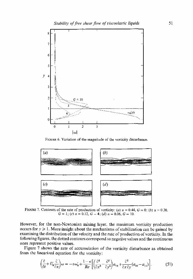
This conclusion is confirmed by looking at the magnitude of the vorticity disturbance (figure 6). Because the eigenfunctions have been arbitrarily normalized, only the trends in this plot should be considered significant. Figure 6 shows that in the limit of an inviscid fluid, the region of maximum magnitude of vorticity production is 0 < y < 1.




0 1 2 3

Id FIGURE 6. Variation of the magnitude of the vorticity disturbance.

I

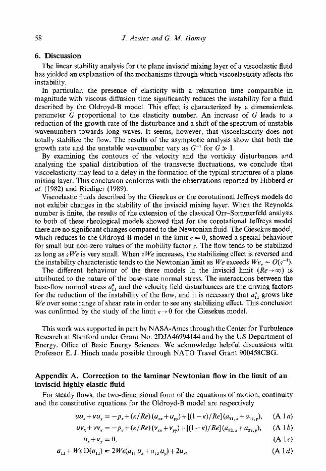
FIGURE 7. Contours of the rate of production of vorticity: (u) a = 0.44, G = 0; (6) a = 0.30, G = 1 ; (c ) a = 0.12, G = 4; (d ) cc = 0.06, G = 10.

However, for the non-Newtonian mixing layer, the maximum vorticity production occurs for y 2 I. More insight about the mechanisms of stabilization can be gained by examining the distribution of the velocity and the rate of production of vorticity. In the following figures, the dotted contours correspond to negative values and the continuous ones represent positive values.

Figure 7 shows the rate of accumulation of the vorticity disturbance as obtained from the linearized equation for the vorticity :




(iil (iiil

FIGURE 8. Contours of the velocity perturbations: (a) streamwise velocity disturbance, u ; (b) transverse velocity disturbance, 21; (i) CL = 0.45, G = 0: (ii) CL = 0.30, G = 1; (iii) CL = 0.10, G = 5 .

We see that in the limit of an inviscid fluid (G = 0), there are two distinct regions. In the first one, in the downstream half-wavelength, the rate of production of vorticity is negative in the upper flow and positive in the lower flow. Keeping in mind that the base-state vorticity is negative, we conclude that the upper flow has a higher vorticity than the lower one and tends to roll into the lower part. The opposite trend is taking place in the upstream half-wavelength where the lower part of the flow tends to roll into the upper part. This is obviously the starting of the well-known mechanism of roll-up. As G increases, the extent of these two regions where the rate of production of vorticity has different signs in the upper and lower parts of the flow is significantly decreased. This is due to the introduction of a spatial phase shift due to finite elasticity and suggests that the roll-up will be slower to appear in the case of an elastic flow.

These conclusions are confirmed by considering the velocity contours (figure 8). In the inviscid case, there is a region in the middle of the domain where the streamwise velocity perturbation ZI is positive in the upper part of the flow and negative in the lower part. This has the effect of increasing the local vorticity and corresponds to the roll-up. This remark is verified by looking at contours of u (figure 8b) : the flow tends to move up in the right half of the figure and down in the left half. For G = 5 , the velocity perturbation u is almost zero in the middle of the domain while elsewhere it has the same sign in both the upper and lower streams. By examining the contours for v, one may surmise that the flow tends to roll-up rather slowly. These predictions conform with the experimental results obtained by Hibberd ef a/. (1982) and Riediger (1989) who noticed that the formation of the typical structures of a plane mixing layer is delayed in the presence of polymer additives and inhibited when a surfactant is added to the flow.

5.2. Corotatiorznl Jeffreyls model The modified Orr-Sommerfeld equation for the corotational Jeffreys model was solved using orthogonal shooting as described in 54. We carried out the calculations for a fixed value of K = 0.5 and two values of the Reynolds number: Re = 100 and 400. Figures 9(n) and 9(h) depict the variations of the growth rates with the wavenumber of the disturbance for various values of the Weissenberg number We. We find that the



160

120

x 1 0 - 3 80

40

0

160

120

g ~ 1 0 3 80

40

0

Stability of free shear $ow of viscoelastic liquids 53

I I I I I 0 0.2 0.4 0.6 0.8

ci

- I

. i I 1 I I 0 0.2 0.4 0.6 0.8

a

FIGURE 9. Instability characteristics for the corotational Jeffreys model for (a) Re = 100, (b) Re = 400.



54

160

120

x 10-3

80

40

0

160

120

c r ~ 10-3 80

40

0

J . Azaiez and G. M . Homsy

I I I I 0 0.2 0.4 0.6 0.8

cc

I I I I I

0 0.2 0.4 0.6 0.8 d

FIGURE 10(a,b). For caption see facing page.




r x 10

0 0.2 0.4 0.6 0.8 a

FIGURE 10. Instability characteristics for the Giesekus model for (a) s = (6) s = 0.3, Re = 100; (c ) s = 0.01, Re = 100. K = 0.5.

Re = lo4;

overall behaviour of the instability is unchanged as compared to the Newtonian limit and the trend is toward the inviscid case for all W e as Re increases. Furthermore, there is little variation with the Weissenberg number indicating that the instability is insensitive to viscoelastic effects of fluids described by the Jeffreys model for this range of parameters. When compared to the previous results, this contrasting behaviour confirms our idea that the effect of viscoelasticity depends critically on how the base- state first and second normal stresses behave as a function of We.

5.3. Giesekus model The modified Orr-Sommerfeld code for the Giesekus model was checked by reproducing the dispersion curves in the limit of a purely Newtonian fluid ( K = 1). A more stringent check was done by reproducing the results for the inviscid mixing layer described by the Oldroyd-B model (S = 0, Re+m and We+co). For this purpose we fixed s = and Re = lo4. Figure lO(a) shows the characteristic curves for various values of We. By comparison with figure 2, it is obvious that it provides a good correspondence with the inviscid results obtained for the Oldroyd-B model.

Figures 10(b) and 1O(c) display the instability characteristics for s = 0.3 and 0.01. We note that for these values of the mobility factor, viscoelasticity does not seem to have a significant effect on the stability of the flow. Varying W e results in either slight stabilization or destabilization, but the shifts from the Newtonian case are always small. For smaller values of s (lop4 and lo-') the instability of the flow is decreased as W e is increased. However, beyond a limiting value of the Weissenberg number We,,




depending upon 5, this trend of stabilization is reversed. Figures Il(a) and l l (b) illustrate this non-monotonic dependence on We.

5.3.1. The limit s = 0

(28) one can obtain expressions of the first and second normal stresses: For s identically equal to zero, the model reduces to the Oldroyd-B equation. From

I 1-A2 N," = - a!2 =

id We[l+(1-2s)A]'

We[l+(l -s)A] ' A - 1 - N," = a& -

It is revealing to examine closely the expression for A in (29). The parameter s appears in the form of the product sWe, so, in order to recover the Oldroyd-B limit it is insufficient to take the limit s --f 0 independently of the values of s We. We examine the two cases that arise when s + 0 :

Case A : s+O and sWe 4 1 From (29) we obtain

A' = 1 -4~We~04+o(sWe~) . (53)

Inserting this expression in (52) yields

N,O = 2Wew;+O(s), N," = -sWewi+o(s), (54)

which, in the limit s --f 0, corresponds to the first and second normal stresses predicted by the Oldroyd-B model.

Case B: s+O and sWe % 1 In this limit (29) gives

Inserting this expression in (52) we obtain

For We sufficiently large, N," N 0 while N," N Jwoli. In this limit, the stabilizing effect tends to disappear and the spectrum of unstable wavenumbers starts getting larger. The stabilizing trend is reversed for a critical Weissenberg number We, for which N: - We. From the expression for NP in (56) this gives ?We: = O(1), which is in quantitative agreement with the results in figure 11. For even larger values of We, N i - 0 and N; - 0, and the characteristic curve tends towards the Newtonian limit.

This analysis and results such as those of figures ll(a) and I l (b) suggest the conjecture that as We is increased for a fixed mobility factor S, the first normal stress N! approaches the value Wew,, and the instability of the flow is reduced. The stabilizing effect then diminishes for values of the Weissenberg number larger than We, since the base-state normal stresses tend to zero and the flow behaves like a Newtonian mixing layer. This suggests that, for a given fluid, there may exist an optimal degree of stabilization which is reached at a particular speed.



160

120

x 10-3 80

40

0

160

120

(T x 10-3

80

40

c

Stability of free shear f low of viscoelastic liquids

I I I I I

.i i

I I I I I 0 0.2 0.4 0.6 0.8

a

57

FIGURE 11. Instability characteristics for the Giesekus model for (a) s = lo-', Re = 100; (b) s = lo-*, Re = 1000. x = 0.5.




6. Discussion The linear stability analysis for the plane inviscid mixing layer of a viscoelastic fluid

has yielded an explanation of the mechanisms through which viscoelasticity affects the instability.

In particular, the presence of elasticity with a relaxation time comparable in magnitude with viscous diffusion time significantly reduces the instability for a fluid described by the Oldroyd-B model. This effect is characterized by a dimensionless parameter G proportional to the elasticity number. An increase of G leads to a reduction of the growth rate of the disturbance and a shift of the spectrum of unstable wavenumbers towards long waves. It seems, however, that viscoelasticity does not totally stabilize the flow. The results of the asymptotic analysis show that both the growth rate and the unstable wavenumber vary as G-l for G + 1 .

By examining the contours of the velocity and the vorticity disturbances and analysing the spatial distribution of the transverse fluctuations, we conclude that viscoelasticity may lead to a delay in the formation of the typical structures of a plane mixing layer. This conclusion conforms with the observations reported by Hibberd et al. (1982) and Riediger (1989).

Viscoelastic fluids described by the Giesekus or the corotational Jeffreys models do not exhibit changes in the stability of the inviscid mixing layer. When the Reynolds number is finite, the results of the extension of the classical Orr-Sommerfeld analysis to both of these rheological models showed that for the corotational Jeffreys model there are no significant changes compared to the Newtonian fluid. The Giesekus model, which reduces to the Oldroyd-B model in the limit s = 0, showed a special behaviour for small but non-zero values of the mobility factor s. The flow tends to be stabilized as long as s We is very small. When s We increases, the stabilizing effect is reversed and the instability characteristic tends to the Newtonian limit as We exceeds Wec - O(s-').

The different behaviour of the three models in the inviscid limit (Re+co) is attributed to the nature of the base-state normal stress. The interactions between the base-flow normal stress ayl and the velocity field disturbances are the driving factors for the reduction of the instability of the flow, and it is necessary that ayl grows like We over some range of shear rate in order to see any stabilizing effect. This conclusion was confirmed by the study of the limit s+O for the Giesekus model.

This work was supported in part by NASA-Ames through the Center for Turbulence Research at Stanford under Grant No. 2DJA46994144 and by the US Department of Energy, Office of Basic Energy Sciences. We acknowledge helpful discussions with Professor E. J. Hinch made possible through NATO Travel Grant 900458CBG.

Appendix A. Correction to the laminar Newtonian flow in the limit of an inviscid highly elastic fluid

and the constitutive equations for the Oldroyd-B model are respectively For steady flows, the two-dimensional form of the equations of motion, continuity

uu,+vu, = -P,+~~/~e)(u~,+~,,)+[(~-K)/~el(~*,,.+~l,,,), (A 1 4 uvx+vv, = -Py+(K/Re)(vxx+ ~ , , > + [ ( ~ - ~ ~ / ~ ~ 1 ~ ~ 1 2 , , + ~ 2 2 , , ~ ~ (A 1b)

(A 1 4

(A 1 4

u,+ vy = 0,

a,, + We D(a,,) = 2We(a11 u,+ a,, u,) + 2ux,




a,, + We D(a,,) = 2 We(a,, v,+ a,, vv) + 2v,,

a12 + We D(a,,) = We(a,, v,+ uZ2 u,,) + (uy + v,), where Re is the Reynolds number, We the Weissenberg number, K = h,/h and D is the convective operator (u8,+ vC:,,). The variables in the above equations are already dimensionless. In the mixin la er, we use the following scaling: y = y / s , x = x, v = v/e and u = u where e = l/ReX.

Let aij = Web,, E = We/Re = e2 We and G = (1 - K ) E. The previous equations are recast in the form

B Y

uu,+vuy = -P:~+~E”~, ,+~yU/~:2)+G(bl , , .+b, , , y /~) , (A 2 4

(A 2b)

u,+vy = 0, (A2 c>

(A 2 4

(A 2 4

(A 2f)

~(uu) , + VV,) = - p y / ~ + K ~ ~ ( v , , + V , , / E ~ ) + G(b,,,, + bsa,,/E),

b,, + We D(b,,) = 2We(b,, u, + b,, u,/E) + (2/ We) u,,

b2, + We Dih,,) = 2 We(eb,, v, + b,, ti,) + (2/ We) v,,

1 We

b,, + We Dib,,) = We(eb,, V , + b,, u J e ) + __ (uY/e + E V J .

Let b,, = b:, E and b,, = b,*, e2, then

MU, + my = - p , + K U ~ ~ + G(b,,,, + bT2) + K F ’ U , ~ , (A 3 4

(A 3 b)

(A 3c)

(A 3 4

(A 3 4

(A 3n

E(UV, + VV,) = -py/e + K ~ u ~ ~ + Ge(b,,, + b:,) + K E ~ V , , -py/e,

24, + v, = 0,

bll + ( E / e 2 ) D(bll) = ~ ( E / E ’ ) (b,, u, + bT2 uy) + ( 2 2 / E ) us,

b,*, + (El&’) D(bz2) = 2(E/&’) (b:, u,+ b& vY) + ( 2 / E ) v,,

h& + (E/e2) D(h&) = ( E / e 2 ) (b,, V , + b;, uY) + ( 1 / E ) (uy + E~v,).

We use the similarity variable, y = y / d , and take the streamfunction, to the first order, equal to 1C.O = E xif(a). The corresponding streamwise and transverse velocities are

uo = f’(y), vo = (y.T(q) - . K V ) ) / ( 2 X 9 . (A 4)

Note that from the momentum equation for u we have p y = 0 + O(e2). The next step is the (usual tentative) expansion of the variables:

(A 5 4 b) A(?) B(V) u = uO+e2----+o(s2), 1) = 2;0+e2T+n(E~), X XT

h, I , g and f satisfy the following equations:

2(1 - ~ ) E w - ~ h ’ ) + 2 ~ f ” ’ + f f N = 0, Jh’ = 2f”(qh-g), (A 6a, b)

(A 6 4

(A 6 4

- (21f‘ +fl’) = 27lf” + g ( f - 77 - $.f”),

- ( f ’g +fg’) = 2lf” + h ( f - ‘ r f ’ - y’f”),



60

with the boundary conditions :

J . Azaiez and G. M . Hornsy

f ( O ) = O , f ’ ( + C O ) = l , f ’(-a)=-1,

h’(0) = g’(0) = Z’(0) = 0,

y(A 6 d ) - (A 6 ~ ) + : (qh -g) (f- yf’ - y’?) = 2ff‘ +fl’ - y(fg)’.

Let X = yh-g; then the system of differential equations reads

2( 1 - K ) E(X’ - h) + 2Kf”’ +ff” = 0, (A 8 4

(A 8b)

(A 8 4

(A 8 4

f h’ = 2 X f ,

X ( f - y . 7 - y”) = 21f’ + f 1’ - q(,f(yh - X))’,

- ( f lqh - X))’ = 21f” + hcf- 6‘ - 7”).

2~ f ” ’ + ( 1 + 2G)ff” = 0

The solution of this system is given by

(A 9 4 X=j’f’, h = f ” 9 1 = i(J” + y 2 . f 2 - 2 r . m (A 9 k d )

with the boundary condition: f(0) = 0, f’( + a> = 1, f’( - a) = - 1. The Newtonian limit is accessible by allowing K to go to 1 (no polymer viscosity) and it is easy to verify that the limit ( K = 1 * G = 0) gives the Blasius equation.

If we define g such thatf(7) = g{[(2G + 1 ) / 4 71, then g satisfies the Blasius equation and thus the solution of the differential equation for f can be mapped to the Blasius solution for 0 < K < 1.



Stability of free shear .flow of viscoelastic liquids 61

Using the usual normal-mode analysis : Q = qo( y) + q( y) e(iax+flz'r-act) and letting D = dldy we have

ia(U,-c)u+ Ubu = -iap+G(iab,,+b~,+ipb,,), (B 3 4 (B 3b) (B 3 4

iau+Dv+pw = 0, (B 3 4 (B 3e) (B 3 f ) (B 3 g )

ia( U, - c) u = - Dp + G(iab,, + b& + ipb,,), ia( U, - c) w = - ipp + G(iab,, + bia + ipb,,),

ia( U, - c) b,, = iaby, v + U{ bZ2, ia( U, - c) b,, = iaby, w + Ui b32,

& = (a"+2)i, 26 = au+pw, 6 = u ; (B 4 4 OI& =PI.., (B 4b)

G"= G, (B 4 4

ia( U, - c) b,, + b;; v = 2iaby, u+ 2Ui b12,

ia( U, - c) b,, = 0, ia( U, - c) b,, = 0, ia( U, - c) b,, = 0, (€3 3 h-j) with the boundary conditions : v + 0 as y --f 5 GO. Let

kb",, = a'b,, + 2/3ab1,+ p 2 b,,, = ab,, + /i'b23, b2J& = b,,/a, (B 4c)

then the system of equations (B 3) can be combined to give the equivalent two- dimensional problem :

i&(U,-e)ii+ U ~ C = -iiij+G(i~ib",,+b"~,), (B 5 4 i&(V,-c)v" = -D~+~(i&b",,+b"~,), (B 5b)

(B 5c) i&(U,--c)bl1+b;iv" = 2iBb~,6+2U~b",,, (B 5 4

iL(U,-c)b",, = iZ&fi+ ~ h b " ~ ~ , (B 5 e ) i & ( q - ~ ) b " ~ ~ = 0, (B 5 f )

iEii + Dv" = 0,

with the boundary conditions v" --f 0 as y --f +_ 03.

Thus we see that the linear theory for the inviscid viscoelastic mixing layer described by the Oldroyd+B rheological model in the special limit We/Re = O(1) does not distinguish between two- and three-dimensional modes. This is, as far as we know, a new result equivalent to the fact that the Rayleigh stability equation holds equally for two- and three-dimensional modes. Furthermore, it is possible to show (Azaiez 1993) that a Squire's transformation exists for the viscous three-dimensional equations for the Oldroyd-B model; however, no theorem can be proven because there exist viscous modes where the growth rates depend upon viscosity, elasticity and first normal stress levels in different ways.

Appendix C. Derivation of stability equations for the corotational Jeffreys model

The linearized equations for the corotational Jeffreys model are

ia((U,-c)(D2-a~)-DD2U,)--(D2-a2)2 Q = --[(D2+aa") a,,+iaD(u,,-a,,)], 1 l;: K

Re

(C l a ) (C 1b) (C 1c) (C 1 4

So a,, = [(D' + a2) + ia We u;; + We .;,(az - Dz)] q5 - w0 We $(azz - a,,), So a,, = [2iaD + ia We u!; - a;2 We(a2 - D')] Q - wo We a,,, So a', = [ - 2iaD + ia We a& + ay2 We(a2 - D')] Q + wo We a12,

3 FLM 268




where S, = 1 +iaWe(U,-c) and D = d/dy. Note that we have used the relation ui2 = -ayl. Subtracting (C I d ) from (C Ic) yields

(C 2) [a!, We D2 + 2iaD + We HI

u22-i.lll = -2 + + 20, w e 5. s o so

Inserting (C 2) into (C 1 b) gives

[a!, We D2 + 2iaD + We HI 4, (C 3 so oo We T

U I 2 =-["D2+P]$+-

where N = 1 - We a!l,

P = We(iaayi + a2u;,) + a2,

H = iaayi - a2a;,,

T = S,2 + 0: We2.

Using (C 3) and (C 4) in the vorticity equation leads to the following modified Orr-Sommerfeld equation :

4

E 4 D i $ = 0 , i=o

where

(C 5 4 a 4 K 1 - K

J , = ia3( V, - c) + - - iawh + __ [(K" + a2K) + ia W e ( F - Q')], Re Re

J=-- -' [2K' + 2ia We(M"+ a2M) -ia We(Q + 2ia WeL'-F) + 2 - Re

J , = (X"+aZX)+K+4ia WeM'+ia We

1 a2

s o -2--i(x WeR'+2a2 We2 L ,

X . K 1-K J4 = -+-

Re Re

In these equations we have set




Appendix D. Derivation of stability equations for the Giesekus model The linearized equations for the Giesekus model are

K [ia{(Q - c) ( ~ 2 - - D~&u,> -- ( ~ 2 - a.p] 4

Re

1-K -- - [(D2 + a,) a,, +iaD(a,, - a22)], ( D 1 a) Re

So a,, = [(D2 + a2) +ia We a:; + We + We ai2 D2] q5

+ U; Wea2,-sWea~,(a,,+a,,)-sWea,2(a~l+a~,), (D 1 b) So a,, = [2iaD + ia We a:; + 2ia We a:, D + 2 We ay2 D2] q5

+ 2We U,!, aI2 - 2sWe(ay, a,, + ay2 q2), (D 1 c)

So a22 = [ - 2iaD + ia We a:; - 2ia We a!, D + 2 W e a’a:,] 4

- 2sWe(ai2 a%, + a;, a,,), (D 1 d)

where So = 1 + ia We( V, - c) and D = d/dy. The three equations for the tensor a can be written in the following form:

S12 a12 = [F,, D2 + H121 4 + u: We a2, - s We aY2(a11 + a2J ,

S2, a,, = [G2, D + H,,1 4 - 2s We a12,

S,, = S,+sWe(a~,+a~,), S,, = So+2sWea:,,

S,, = S, + 2s We a:2,

Sll all = [F,, D2 + Gll D + H,,] # + 2We U,!, a,, - 2sWe ay2 a12,

where

F,, = 1 + We ai2,

H,, = a2( 1 + We a!,) + ia W e a!;, F,, = 2 We

Hll = in We a?;, G,, = 2ia( 1 + We a:,),

G,, = - 2ia( 1 + We a:,), H22 = We(2a24, + iaai’,).

Expressing a,, and a22 in terms of a,, gives the following expressions:

Subtracting (D 4 4 from (D 4b) leads to

Introducing (D 4) into (D 2a) gives

a12 = (XD2+ZD+P)4,



64

where

J . Azaiez and G. M . Homsy

’ I We( Uh - say,) We( Uh - sa!,) , N = s We a:, L=----- , M = Sll s, 1 s 2 2

s We a;, Q=- s 2 2 , T = S12+2sWea~, (M+Nj ,

NG,, - LG,, T ’

, z = 42 - L41 T

H12 + NHZZ - LHll , x= T

P =

When we insert (D 6) and (D 5 ) in the vorticity equation, we obtain the following modified Orr-Sommerfeld equation :

4

C GiDi$ = 0, i = O

where

G, = ~ - K [ (Z”+a’Z) + 2P‘ + 2ia{(M’ + Q’) Z+(M+ Q) (Z’ +P)] Re

[ (x” + a2X) + 22 ’ + P a2K (1 - K j

G, = -ia(4-c)-2-+- Re Re

G, =- Re

K 1-K G --+-X.

4 - Re Re

Appendix E. Long-wave instability of a free shear layer of an Oldroyd-B fluid

By E. J , Hinch Department of Applied Mathematics and Theoretical Physics, University of

Cambridge, Silver Street, Cambridge CB3 9EW, UK In the main body of the paper Azaiez & Homsy have shown that the high-Reynolds-

number inertial instability of a free shear layer can be partially stabilized by the elasticity of a non-Newtonian fluid. They found that only the Oldroyd-B fluid could provide the large quadratic normal stresses (tension in the streamlines) comparable



Stability of' free shear flow of viscoelastic liquids 65

with the quadratic Reynolds stresses required for a significant effect at high Reynolds numbers, and that then only the long waves are unstable. Now for long waves the inertial instability of a free shear layer is described by the Kelvin-Helmholtz instability. As the large non-Newtonian stresses are confined to the shear layer, one might anticipate that the stabilizing effect of the normal stresses on the long waves is just that of an elastic membrane or surface tension on the Kelvin-Helmholtz instability. The purpose of this appendix is to analyse this mechanism.

E. 1. Governing equations

v * u = 0,

p- = -VP+,L~V~U+GV*A+J

Consider the flow of an Oldroyd-B fluid governed by

Du Dt

DA 1 - = A . VU + VuT* A +- (A -/), Dt 7

where G is the elasticity modulus and 7 the relaxation rate associated with the polymer stretch A .

The basic state is a unidirectional shear layer of thickness 6 and velocity jump 2U0:

u = (U(y),O) with U = U,tanh(y/S),

with polymer stretch (1 +2(7U')2 ?U')

1 ' A =

7U'

A forcefis needed to maintain the basic state. We make two approximations : large Reynolds number pUo 6/& + G7) 9 1 to

concentrate on the inertial instability; and large Weissenberg number Uo7/J % 1 to provide the large normal stresses. The large Reynolds number allows one to ignore the diffusion of momentum. The large Weissenberg number allows one to ignore the stress relaxation during the instability and to take the elastic stress in the basic state as just the normal stress GA,,. The equations governing the linear instability are then

au av -+- = 0, ax 2y

We now look at a linearized instability where all perturbation quantities are functions of y and proportional to e" with 0 = ia(x- ct) and with growth rate r = aci.




E.2. Inside the thin shear layer

The elastic stress only exists within the shear layer. Introducing the streamfunction 31. with u = V and D = -ia$, we can solve the stress perturbation equations with

Following standard boundary-layer theory for long thin layers, we consider only the x-momentum equation, and set the pressure gradient to zero, because it vanishes to leading order outside the layer and it does not vary across the thin layer. Substituting in the above solution for the stress, we obtain the momentum equation

which is an integral of (18) with a = 0. This momentum equation has the simple solution (cf. (42))

= (U- C) 7 with constant 7 4 8, which gives

u = U’7, D = - ia(U- c) 7, a,, = A;, 7, a,, = -iaA,, 7.

This solution can be interpreted just as a vertical displacement of streamlines from yo to y = yo - 7 ee with 7 $ 6. Conserving the horizontal velocity in this displacement at U(y,) gives in the Eulerian frame a horizontal velocity U( y + 7 e@) = U+ 7 esU’. The vertical velocity is given by the statement that in the long-wavelength limit the displaced streamlines are effectively material surfaces D b + 7 e@)/Dt = 0, so D = - ia( U - c) 7 ee. The normal elastic stress is displaced vertically with the streamlines A,,(y + 7 e@) = A,,(y) + 7 eR& while the shear elastic stress results from the tilt in the streamlines a,, = - iaA,, 7. With this simple solution, the normal stress or tension along the displaced and tilted streamlines is unchanged, and so there is no need to accelerate the fluid along the streamlines.

E.3. Potentialflow outside the shear layer The above solution produces a normal flux out of the shear layer:

D = -ia(k Uo-c)y.

This is precisely the normal velocity in the standard Kelvin-Helmholtz instability of a vortex sheet, and is really only mass conservation, which is possible so long as the momentum balance is not disturbed inside the shear layer. The normal efflux drives a potential flow outside the shear layer with velocity potentials i( & Uo - c) 7 eTay. Hence just outside the shear layers there is a flow in the x-direction:

-a(U, , -c)~ and +a(-U,-c)y.

Note that this flow is O(a) smaller than that in the shear layer, but with no friction acting in the potential region the only mechanism available to drive flow there is the vertical efflux out of the shear layer.



Stability of free shear ,$ow of viscoelastic liquids 67

The acceleration of the above horizontal flow requires a horizontal pressure gradient

Hence there is a pressure difference across the shear layer of

[ p ] = 2/74 u; + c2) 7.

E.4. Hoop stress

Back in the shear layer we must now consider the higher-order effect of the curvature of the tensioned streamlines. In the large-elasticity limit, one can ignore the inertial terms in the y-momentum equation leaving just the elastic stress and the pressure gradient :

Substituting the tilted streamline solution a12 = - i d l , 7, we see that aa,,/ax is just the curvature of the streamlines applied to the basic normal stress All . Integrating the above equation across the shear layer, one finds a jump in the pressure:

[p ] = a2rT with net tension T = G A , , dy. s Now in the basic state

A 11 - - 2r2Uf2 = 2r2Uisech4(y/S)/S2.

Hence the membrane tension is SGr’U; T = -

36 .

Finally, equating this elastic membrane hoop-stress pressure difference to that found earlier in the potential flow just outside the shear layer, we find the dispersion relation for the instability :

which is the square of (48). It also agrees with Lamb for the inviscid Kelvin-Helmholtz instability with surface tension. The dispersion relation has a maximum growth rate

4p u; 3T ’

4pu’ which occurs at a,,, = __ urnas = ~ 3 4 3 T

i.e. in Azaiez & Homsy’s non-dimensionalization crnaz = 0.289G-1 (cf. their 0.308G-lj at amaz = 0.5G-1 (cf. their 0.581G-l), which are in better agreement with the exact numerical results in figure 4 than the results of 3 5.1.1.

E. 5. Validity

We must now check the various assumptions which have been made. First there the large-elasticity assumption of neglecting the inertial terms compared with the elastic stress in the calculation of the hoop stress from the y-momentum equation. This requires.

paUv < Gaa,,.



68

Substituting in the expressions for u and aI2 leads to the requirement

J. Azaiez and G. M . Hornsy

pa2 4 Gr2

Next there is an assumption that wavelength is long compared with the thickness of the shear layer:

a s 4 1.

For the wavelength at the maximum growth rate this gives, when substituting in the expression of the tension T, the condition pS2 4 Gr2 again.

The assumption that the instability is fast compared with the time for the elastic stress to relax requires

For the maximum growth rate this gives

err% 1 .

pSU, %- Gr,

which is effectively the same as the high-Reynolds-number condition, so long as the elastic stresses make a significant contribution to the effective viscosity, Gr >, p.

To summarize, the analysis needs a large Reynolds number Re = p U,, S / ( p + GT) 9 1, a large Weissenberg number We = U, 7 / S 1, and a high elasticity (to make the long waves the only unstable ones) G72/pS2 = We/& >> 1.

While the basic flow could be maintained by applying a suitable force fieldfin the momentum equation, one would really like to apply the analysis to a quasi-parallel quasi-steady mixing layer, and here there is a problem. At a time t after contact, a mixing layer has a width S(t) scaling with (v* I);, where one would use Y* = Gr /p when Gr >, p. The high-elasticity condition then gives t 4 7, which means that there is insufficient time to establish the quasi-steady basic stress field. Clearly a more detailed analysis near the splitter plate is needed.

This work was completed while E. J. H. was a guest at PMMH, ESPCI, Paris.

R E F E R E N C E S

AZAIEZ, J. 1993 Instability of Newtonian and non-Newtonian free shear flows. PhD thesis, Stanford

BERMAN, N. 1978 Drag reduction by polymers. Ann. Rev. Fluid Mech. 10, 47-64. BETCHOV, R. & SZEWCZYK, A. 1963 Stability of a shear layer between parallel streams. Phys. Fluids

BIRD, R. B., CURTISS, C. F., ARMSTRONG, R. C. & HASSAGER, 0. 1987 Dynamics of Polymeric

BOGER, D. V. 1977 A highly elastic constant-viscosity fluid. J . Non-Newtonian FluidMech. 3, 87-91. BRIS, A. N., ARMSTRONG, R. C. & BROWN, R. A. 1986 Finite element calculation of viscoelastic flow

in a journal bearing. 11. Moderate eccentricity. J. Non-Newtonian Fluid Mech. 19, 323-347. CONTE, S. D. 1966 The numerical solution of linear boundary value problems. SIAM Rev. 8,

CORCOS, G. M. & LIN, S. J. 1984 The mixing layer: deterministic models of a turbulent flow: Part

DRAZIN, P. G. & HOWARD, L. N. 1962 The instability to long waves of unbounded parallel inviscid

DRAZIN, P. G. & REID, W. H. 1981 Hydrodynamic Stability. Cambridge University Press. GIESEKUS, H. 1966 Zur stabilitat von stromungen viskoelastischer flussigkeiten. Rheol. Acta 5 ,

University.

6, 1391-1396.

Liquids, vol. 2, 2nd edn. Wiley-Intersciences.

309-32 1.

2. The origin of the three-dimensional motion. J. Fluid Mech. 139, 67-95.

flow. J . Fluid Mech. 14, 257-283.

239-252.



Stability of free shear ,flow of viscoelustic liquids 69

GESEKUS, H. 1982 A simple constitutive equation for polymer fluids based on the concept of

GIESEKUS, H. 1983 Stressing behavior in simple shear flow as predicted by a new constitutive model

GOUDARD, J. P. 1979 Polymer fluid mechanics. Adv. Appl. Mech. 19, 143-219. HERBERT, T. 1988 Secondary instability of boundary layers. Ann. Rev. Fluid Mech. 20, 487-526. HIBBERD, M. F., KWADE, M. & SCHARF, R. 1982 Influence of drag reducing additives on the

Ho, C., M. & HUERRE, P. 1984 Perturbed free shear layers. Ann. Rev. Fluid Mech. 16, 365424. LARSON, R. G. 1988 Constitutive Equations f o r Polymer Melts and Solutions. Buttenvorths. LING, C. & REYNOLDS, W. C. 1973 Non-parallel flow corrections for the stability of shear flows. J .

Fluid Mech. 59, 571 -591. MACKAY, M. E. & BOGER, D. V. 1987 An explanation of the rheological properties of Boger fluids.

J . Non-Newtonian Fluid Mech. 22, 235-243. METCALPE, R. W., ORSZAG, S. A., BRACHET, M. E., MENON, S. & RILEY, J. J. 1987 Secondary

instability of a temporally growing mixing layer. J . Fluid Mech. 184, 207-243. MICHALKE, A. 1964 On the inviscid instability of the hyperbolic tangent velocity profile. J . Fluid

Mech. 19, 543-556. MOSER, R. D. & ROGERS, M. M. 1991 Mixing transition and the cascade to small scales in a plane

mixing layer. Phys. Fluids A 3, 1128-1 134. RIEDIGER, S. 1989 Influence of drag reducing additives on a plane mixing layer. In Drag Reduction

in FZuid Flows (ed. R. H. J. Sellin & R. J. Moses), pp. 303-310. Ellis Honvood. SCHARF, R. 1 9 8 5 ~ Die wirkung von polymerzusatzen auf die turbulenzstruktur in der ebenen

mischungsschicht zweier strome. I Beeinflussung der integralen KenngroDen des turbulenzfeldes. Rheol. Acta 24. 272-295.

SCHARF, R. 1985b Die wirkung von polymerzusatzen auf die turbulenzstruktur in der ebenen mischungsschicht zweier strome. 11 Korrelationsanalyse der mischungsschicht wirbelstruktur. Rheol. Actu 24, 38541 1.

SCHLEINIGER, G. & WEINACHT, R. J. 1991 A remark on the Giesekus viscoelastic fluid. J. Rheol. 35,

SQUIRE, H. B. 1933 On the stability of three-dimensional disturbances of viscous fluid flow between

TATSUMI, T. & GOTOH, K. 1959 The stability of free boundary layers between two uniform streams.

deformation-dependent tensorial mobility. J. Non-Newtonian Fluid Mech. 11, 69-1 09.

for polymer fluids. J. Non-Newtonian Fluid Mech. 12, 367-374.

structure of turbulence in a mixing layer. Rheol. Acta 21, 582-586.

1157-1 170.

parallel walls. Proc. R . Soc. Lond. A 142, 621-628.

J. Fluid Mech. 7, 433441.


Date post:	25-May-2020
Category:	Documents
Upload:	others
View:	3 times
Download:	0 times

Linear stability of free shear flow of viscoelastic liquids · 2009-07-21 · Linear stability of...

Documents