LINEAR SUPERPOSITION IN NONLINEAR WAVE …afigotin/papers/Babin Figotin LINEAR... · LINEAR...

November 28, 2006 11:15 WSPC/148-RMP J070-00285

Reviews in Mathematical PhysicsVol. 18, No. 9 (2006) 971–1053c© World Scientific Publishing Company

LINEAR SUPERPOSITION IN NONLINEAR WAVE DYNAMICS

A. BABIN∗ and A. FIGOTIN†

Department of Mathematics, University of California at Irvine,CA 92697, USA

∗[email protected]†[email protected]

Received 24 April 2006Revised 27 August 2006

We study nonlinear dispersive wave systems described by hyperbolic PDE’s in Rd and

difference equations on the lattice Zd. The systems involve two small parameters: one is

the ratio of the slow and the fast time scales, and another one is the ratio of the smalland the large space scales. We show that a wide class of such systems, including non-linear Schrodinger and Maxwell equations, Fermi–Pasta–Ulam model and many othernot completely integrable systems, satisfy a superposition principle. The principle essen-tially states that if a nonlinear evolution of a wave starts initially as a sum of genericwavepackets (defined as almost monochromatic waves), then this wave with a high accu-racy remains a sum of separate wavepacket waves undergoing independent nonlinearevolution. The time intervals for which the evolution is considered are long enough toobserve fully-developed nonlinear phenomena for involved wavepackets. In particular,our approach provides a simple justification for numerically observed effect of almostnon-interaction of solitons passing through each other without any recourse to the com-plete integrability. Our analysis does not rely on any ansatz or common asymptoticexpansions with respect to the two small parameters but it uses rather explicit and

constructive representation for solutions as functions of the initial data in the form offunctional analytic series.

Keywords: Nonlinear waves; wave packets; quasiparticles; nonlinear hyperbolic PDE;nonlinear Schrodinger equation; Fermi–Pasta–Ulam system; dispersive media; smallparameters; implicit function theorem.

Mathematics Subject Classification 2000: 35L70, 35L75, 35L90, 35G55, 35Q60, 34C15,37K60, 39A12

1. Introduction

The principal object of our studies here is a general nonlinear evolutionary sys-tem which describes wave propagation in homogeneous media governed either bya hyperbolic PDE’s in Rd or by a difference equation on the lattice Zd, where

971


972 A. Babin & A. Figotin

d = 1, 2, 3, . . . is the space dimension. We assume the evolution to be governed bythe following equation with constant coefficients

∂τU = − i�L(−i∇)U + F(U), U(r, τ)|τ=0 = h(r), r ∈ Rd, (1.1)

where (i) U = U(r, τ), r ∈ Rd, U ∈ C2J is a 2J-dimensional vector; (ii) L(−i∇)is a linear self-adjoint differential (pseudodifferential) operator with constant coef-ficients with the symbol L(k), which is a Hermitian 2J × 2J matrix; (iii) F is ageneral polynomial nonlinearity; (iv) � > 0 is a small parameter. The form of theequation suggests that the processes described by it involve two time scales. Sincethe nonlinearity F(U) is of order one, nonlinear effects occur at times τ of orderone, whereas the natural time scale of linear effects, governed by the operator Lwith the coefficient 1/�, is of order �. Consequently, the small parameter � measuresthe ratio of the slow (nonlinear effects) time scale and the fast (linear effects) timescale. A typical example an equation of the form (1.1) is nonlinear Schrodingerequation (NLS) or a system of NLS. Another one is the Maxwell equation in aperiodic medium when truncated to a finite number of bands, and more examplesare discussed below.

We assume further that the initial data h for the evolution equation (1.1) to bethe sum of a finite number of wavepackets hl, l = 1, . . . , N , i.e.

h = h1 + · · · + hN , (1.2)

where the monochromaticity of every wavepacket hl is characterized by anothersmall parameter β.

The well-known superposition principle is a fundamental property of every linearevolutionary system, stating that the solution U corresponding to the initial data has in (1.2) equals

U = U1 + · · · + UN , for h = h1 + · · · + hN , (1.3)

where Ul is the solution to the same linear problem with the initial data hl.Evidently the standard superposition principle cannot hold exactly as a gen-

eral principle in the presence of a nonlinearity, and, at the first glance, there is noexpectation for it to hold even approximately. We have discovered though that thesuperposition principle does hold with a high accuracy for general dispersive non-linear wave systems provided that the initial data are a sum of generic wavepackets,and this constitutes the subject of this paper. Namely, the superposition principlefor nonlinear wave systems states that the solution U corresponding to the multi-wavepacket initial data h as in (1.2) equals

U = U1 + · · · + UN + D, for h = h1 + · · · + hN , where D is small.

As to the particular form (1.1) we chose to be our primary one, we would like topoint out that many important classes of problems involving small parameters canbe readily reduced to the framework of (1.1) by a simple rescaling. It can be seenfrom the following examples. First example is a system with a small factor before


Linear Superposition in Nonlinear Wave Dynamics 973

the nonlinearity

∂tv = −iLv + αf(v), v|t=0 = h, 0 < α � 1, (1.4)

where initial data are bounded uniformly in α. Such problems are reduced to (1.1)by the time rescaling τ = tα. Note that now � = α and the finite time interval0 ≤ τ ≤ τ∗ corresponds to the long time interval 0 ≤ t ≤ τ∗/α.

The second example is a system with small initial data on a long time interval.The system here is given and has no small parameters but the initial data are small,namely

∂tv = −iLv + f0(v), v|t=0 = α0h, 0 < α0 � 1, where

f0(v) = f (m)0 (v) + f (m+1)

0 (v) + · · · , (1.5)

where α0 is a small parameter and f (m)(v) is a homogeneous polynomial of degreem ≥ 2. After the rescaling v = α0V, we obtain the following equation with a smallnonlinearity

∂tV = −iLV + αm−10 [f (m)

0 (V) + α0f0(m+1)(V) + · · ·], V|t=0 = h, (1.6)

which is of the form of (1.4) with α = αm−10 . Introducing the slow time variable

τ = tαm−10 we get from the above an equation of the form (1.1), namely

∂τV = − iαm−1

0

LV + [f (m)(V) + α0f (m+1)(V) + · · ·], V|t=0 = h, (1.7)

where the nonlinearity does not vanish as α0 → 0. In this case � = αm−10 and the

finite time interval 0 ≤ τ ≤ τ∗ corresponds to the long time interval 0 ≤ t ≤ τ∗αm−1

0

with small α0 � 1.Very often in theoretical studies of equations of the form (1.1) or ones reducible

to it, a functional dependence between � and β is imposed, resulting in a singlesmall parameter. The most common scaling is � = β2. The nonlinear evolutionof wavepackets for a variety of equations which can be reduced to the form (1.1)was studied in numerous physical and mathematical papers, mostly by asymp-totic expansions of solutions with respect to a single small parameter similar toβ, see [11, 14, 18, 20, 23, 28, 29, 34, 38–40] and references therein. Often the asymp-totic expansions are based on a specific ansatz prescribing a certain form to thesolution. In our studies here we do not use asymptotic expansions with respectto a small parameter and do not prescribe a specific form to the solution, butwe impose conditions on the initial data requiring it to be a wavepacket or alinear combination of wavepackets. Since we want to establish a general prop-erty of a wide class of systems, we apply a general enough dynamical approach.There is a number of general approaches developed for the studies of high-dimensional and infinite-dimensional nonlinear evolutionary systems of hyperbolictype, [10, 13, 19, 22, 27, 31, 35, 39, 41, 43, 45] and references therein. We develop here



an approach which allows to exploit specific properties of a certain class of initialdata, namely wavepackets and their linear combinaions, which comply with thesymmetries of equations. Such a class of the initial data is obviously lesser thanall possible initial data. One of the key mathematical tools developed here for thenonlinear studies is a refined implicit function theorem (Theorem 4.25). This theo-rem provides a constructive and rather explicit representation of the solution to anabstract nonlinear equation in a Banach space as a certain functional series. Therepresentation is explicit enough to prove the superposition principle and is generalenough to carry out the studies of the problem without imposing restrictions ondimension of the problem, structural restrictions on nonlinearities or a functionaldependence between the two small parameters �, β.

As we have already stated the superposition principle holds with high accuracyfor linear combinations of wavepackets. A wavepacket h(β, r) can be most easilydescribed in terms of its Fourier transform h(β,k). Simply speaking, wavepacketh(β,k) is a function which is localized in β-neighborhood of a given wavevectork∗ (the wavepacket center) and as a vector is an eigenfunction of the matrix L(k),details of the definition of the wavepacket can be found in the following Sec. 2. Thesimplest example of a wavepacket is a function of the form

h(β,k) = β−dh

(k − k∗

β

)gn(k∗), k ∈ Rd, (1.8)

where gn(k∗) is an eigenvector of the matrix L(k∗) and h(k) is a Schwartz function(i.e. it is infinitely smooth and rapidly decaying one). Note that the inverse Fouriertransform h(β, r) of h(β,k) has the form

h(β, r) = h(βr)eik∗rgn(k∗), r ∈ Rd, (1.9)

where h(r) is a Schwartz function, and obviously has a large spatial extension oforder β−1.

We study the nonlinear evolution equation (1.1) on a finite time interval

0 ≤ τ ≤ τ∗, where τ∗ > 0 is a fixed number (1.10)

which may depend on the L∞ norm of the initial data h but, importantly, τ∗does not depend on �. We consider classes of initial data such that wave evolutiongoverned by (1.1) is significantly nonlinear on time interval [0, τ∗] and the effect ofthe nonlinearity F (U) does not vanish as � → 0. We assume that β, � satisfy

0 < β ≤ 1, 0 < � ≤ 1,β2

�≤ C1 with some C1 > 0. (1.11)

The above condition on the dispersion parameter β2

� ensures that the disper-sive effects are not dominant and do not suppress nonlinear effects, see [7] for adiscussion.

To formulate the superposition principle more precisely, we introduce first thesolution operator S(h)(τ) : h → U(τ) which relates to the initial data h of the non-linear evolution equation (1.1) the solution U(t) of this equation. Suppose that the



initial state is a multi-wavepacket, namely h =∑

hl, with hl, l = 1, . . . , N being“generic” wavepackets. Then for all times 0 ≤ τ ≤ τ∗ the following superpositionprinciple holds

S(

N∑l=1

hl

)(τ) =

N∑l=1

S(hl)(τ) + D(τ), (1.12)

‖D(τ)‖E = sup0≤τ≤τ∗

‖D(τ)‖L∞ ≤ Cδ�

β1+δfor any small δ > 0. (1.13)

Obviously, the right-hand side of (1.13) may be small only if � ≤ C1β. There areexamples (see [7]) in which D(τ) is not small for � = C1β. In what follows we referto a linear combination of wavepackets as a multi-wavepacket, and to wavepacketswhich constitutes the multi-wavepacket as component wavepackets.

The superposition principle implies, in particular, that in the process of non-linear evolution every single wavepacket propagates almost independently of otherwavepackets even though they may “collide” in physical space for a certain periodof time and the exact solution equals the sum of particular single wavepacket solu-tions with a high precision. In particular, the dynamics of a solution with multi-wavepacket initial data is reduced to dynamics of separate solutions with singlewavepacket data. Note that the nonlinear evolution of a single wavepacket solu-tion for many problems is studied in detail, namely it is well-approximated by itsown nonlinear Schrodinger equation (NLS), see [18, 23, 29, 30, 39–41,7]and refer-ences therein.

The superposition principle (1.12), (1.13) can also be looked at as a form ofseparation of variables. Such a form of separation of variables is different from usualcomplete integrability, and its important factor is the continuity of spectrum of thelinear component of the system. The approximate superposition principle imposescertain restrictions on dynamics which differ from usual constraints imposed by theconserved quantities as in completely integrable systems as well as from topologicalconstraints related to invariant tori as in KAM theory.

Now we present an elementary physical argument justifying the superpositionprinciple. If nonlinearity is absent, the superposition principle holds exactly andany deviation from it is due to the nonlinear interactions between wavepackets, sowe need to estimate their impact. Suppose that initially at time τ = 0 the spatialextension s of every composite wavepacket is characterized by the parameter β−1 asin (1.9).] Assume also (and it is quite an assumption) that the component wavepack-ets during the nonlinear evolution maintain somehow their wavepacket identity,group velocities and spatial extension. Then, consequently, the spatial extensionof every component wavepacket is propositional to β−1 and its group velocity vj

is proportional to �−1. The difference ∆v between any two different componentgroup velocities is also proportional to �−1. The time when two different compo-nent wavepackets overlap in space is proportional to s/|∆v| and, hence, to �/β.



Since the nonlinear term is of order one, the magnitude of the impact of the nonlin-earity during this time interval should be proportional to �/β, which results in thesame order of magnitude of D. This conclusion is in agreement with the estimateof magnitude of D in (1.13) (if we set δ = 0).

The rigorous proof of the superposition principle we present in this paper is notbased on the above argument since it implicitly relies on a superposition principle inthe form of an assumption that component wavepackets can somehow maintain theiridentity, group velocities and spatial extension during nonlinear evolution which byno means is obvious. In fact, the question if a wavepacket or a multi-wavepacketstructure can be preserved during nonlinear evolution is important and interestingquestion on its own right. The answer to it under natural conditions is affirmative aswe have shown in [7]. Namely, if initially solution was a multi-wavepacket at τ = 0, itremains a multi-wavepacket at τ > 0, and every component wavepacket maintainsits identity. Therefore a wavepacket can be interpreted as a quasi-particle whichmaintains its identity and can interact with other quasi-particles. This propertyholds also in the situation when there are stronger nonlinear interactions betweenwavepacket components which do not allow the superposition principle to hold, see[7] for details.

The proof we present here is based on general algebraic-functional considera-tions. The strategy of our proof is as follows. First, we prove that the operator S(h)in (1.12) is analytical, i.e. it can be written in the form of a convergent series

S(h) =∞∑

j=1

S(j)(hj), hj = h, . . . ,h (j copies of h),

where S(j)(hj) is a j-linear operator applied to h. Now we substitute h in S(j) withthe sum of hl as in (1.2). Considering for simplicity the case N = 2 and using thepolylinearity of S(j) we get

S(2)((h1 + h2)2) = S(2)((h1)2) + 2S(2)(h1h2) + S(2)((h2)2), . . . ,

implying after the summation

S(h) = S(2)((h1)2) + S(3)((h1)3) + · · · + S(2)((h2)2) + S(3)((h2)3) + · · · + Scr

= S(h1) + S(h2) + Scr,

where Scr is a sum of all cross terms such as S(2)(h1h2) etc. The main part of theproof is to show that every term in Scr is small. An important step for that is basedon the refined implicit function theorem (Theorem 4.25) which allows to representthe operators S(j) in the form of a sum of certain composition monomials, which,in turn, have a relatively simple oscillatory integral representation. Importantly, therelevant oscillatory integrals involve the known initial data hl rather than unknownsolution U. The analysis of the oscillatory integrals shows that there are two mech-anisms responsible for the smallness of the integrals. The first one is time averag-ing, and the second one is based on large group velocities (in the slow time scale) of



wavepackets. Remarkably, if wavepackets satisfy proper genericity conditions, everycross term is small due one of the above mentioned two mechanisms. Importantly,the both mechanism are instrumental for the smallness of terms in Scr, and the timeaveraging alone is not sufficient. We obtain estimates on terms in Scr which ulti-mately yield the estimate (1.13). Since the smallness of interactions between wavesunder nonlinear evolution stems from high frequency oscillations in time and spaceof functions involved in the interaction integrals, we can interpret it as a result of thedestructive wave interference. The above sketch shows that the mathematical toolswe use in our studies are (i) the theory of analytic functions and corresponding seriesof infinite-dimensional (Banach) variable, and (ii) the theory of oscillatory integrals.

We would like to point out that the estimate (1.13) for the remainder in thesuperposition principle is quite accurate. For example, when the estimate is appliedto the sine-Gordon equation with bimodal initial data, it yields essentially opti-mal estimates for the magnitude of the interaction of counterpropagating waves.These estimates are more accurate than ones obtained by the well known ansatzmethod as in [38], and the comparative analysis is provided below in Example 1of Sec. 2.2.

To summarize the above analysis, we list important ingredients of our approach.

• The spectrum of the underlying linear problem is continuous.• The wave nonlinear evolution is analyzed based on the modal decomposition with

respect to the linear component of the system because there is no exchange ofenergy between modes by linear mechanisms. Wavepacket definition is based onthe modal expansion determining, in particular, its the spatial extension and thegroup velocity.

• The problem involves two small parameters β and � respectively in the ini-tial data and coefficients of the equations. These parameters scale respectively(i) the range of wavevectors involved in its modal composition, with β−1 scalingits spatial extension, and (ii) � scaling the ratio of the slow and the fast timescales. We make no assumption on the functional dependence between β and �,which are essentially independent and are subject only to inequalities.

• The nonlinear evolution is studied for a finite time τ∗ which may depend on, say,the amplitude of the initial excitation, and, importantly, τ∗ is long enough toobserve appreciable nonlinear phenomena which are not vanishingly small. Thesuperposition principle can be extended to longer time intervals up to blow-uptime or even infinity if relevant uniform in β and � estimates of solutions inappropriate norms are available.

• Two fast wave processes (in the chosen slow time scale) attributed to the linearoperator L and having typical time scale of order � can be identified as responsi-ble for the essential independence of wavepackets: (i) fast time oscillations whichlead to time averaging; (ii) fast wavepacket propagation with large group veloci-ties produce effective weakening of interactions which are not subjected to timeaveraging.



The rest of the paper is organized as follows. In the following Sec. 2, we for-mulate exact conditions and theorems for lattice equations and partial differentialequations and give examples. In Sec. 3, we recast the original evolution equation ina convenient reduced form allowing, in particular, to construct a representation ofthe solution in a form of convergent functional operator series explicitly involvingthe equation nonlinear term. In Sec. 4, we provide the detailed analysis of function-analytic series used to get a constructive representation of the solution. Section 5is devoted to the analysis of certain oscillatory integrals which are terms of theseries representing the solution. Note that when making estimations we use thesame letter C for different constants in different statements. Finally, the proofs ofTheorems 2.15 and 2.19 are provided in Sec. 6. More examples and generalizationsare given in Sec. 7. For the reader’s convenience, we provide a list of notations inthe end of the paper.

2. Statement of Results

In this section, we consider two classes of problems: lattice equations and partialdifferential equations. After Fourier transform they can be written in the modal formwhich is essentially the same in both cases. We formulate the exact conditions on themodal equations and present the main theorems on the superposition principle. Wealso give examples of equations to which the general theorems apply, in particularFermi–Pasta–Ulam system and nonlinear Schrodinger equation.

2.1. Main definitions, statements and examples for the lattice

equation

The first class of evolutionary systems we consider involves systems of equationsdescribing coupled nonlinear oscillators on a lattice Zd, namely the following latticesystem of ordinary differential equations (ODE’s) with respect to time

∂τU(m, τ) = − i�LU(m, τ) + F (U)(m, τ), U(m, 0) = h(m), m ∈ Zd, (2.1)

where L is a linear operator, F is a nonlinear operator and � > 0 is a smallparameter (see [6]). To analyze the evolution equation (2.1) it is instrumental torecast it in the modal form (the wavevector domain), in other words, to apply to itthe lattice Fourier transform as defined by the formula

U(k) =∑

m∈Zd

U(m)e−im·k, where k ∈ [−π, π]d, (2.2)

k is called a wave vector. We assume that the Fourier transformation of the originallattice evolutionary equation (2.1) is of the form

∂τ U(k, τ) = − i�L(k)U(k, τ) + F (U)(k, τ); U(k, 0) = h(k) for τ = 0. (2.3)

Here, U(k, τ) is 2J-component vector, L(k) is a k-dependent 2J × 2J matrix thatcorresponds to the linear operator L and F (U) is a nonlinear operator, which we



describe later. The matrix L(k) and the coefficients of the nonlinear operator F (U)in (2.3) are 2π-periodic functions of k and for that reason we assume that k belongsto the torus Rd/(2πZ)d which we denote by [−π, π]d. The k-dependent matrix L(k)determines the linear operator L and plays an important role in the analysis. Werefer to L(k) as to the linear symbol. Since (2.3) describes evolution of the Fouriermodes of the solution, we call (2.3) modal evolution equation.

We study the modal evolution equation (2.3) on a finite time interval

0 ≤ τ ≤ τ∗, (2.4)

where τ∗ > 0 is a fixed number which, as we will see, may depend on the magnitudeof the initial data. The time τ∗ does not depend on small parameters, it is of orderone and is determined by norms of operators and initial data; it is almost optimalfor general F since there are examples when τ∗ is of the same order as the blow-uptime of solutions. To make formulas and estimates simpler, we assume without lossof generality that

τ∗ ≤ 1. (2.5)

For a number of reasons the modal form (2.3) of the evolution equation is muchmore suitable for nonlinear analysis than the original evolution equation (2.1). Thisis why from now on we consider the modal form of evolution equation (2.3) for themodal components U(k, τ) as our primary evolution equation.

First, as an illustration, let us look at the simplest nontrivial example of (2.3)with J = 1 corresponding to two-component vector fields on the lattice Zd. Atwo-component vector function U(m) of a discrete argument m ∈ Zd has the form

U(m) =[

U+(m)U−(m)

], m ∈ Zd. (2.6)

In this example L(k) in (2.3) is a 2×2 matrix, and we assume that for almost all kit has two different real eigenvalues ω−(k) and ω+(k) (the dependence of ω±(k) onk is called the dispersion relation) satisfying the relation ω−(k) = −ω+(k), namely,

L(k)gζ(k) = ωζ(k)gζ(k), ωζ(k) = ζω(k), ζ = ±, (2.7)

where, evidently, gζ(k) are the eigenvectors of L(k). These eigenvalues ωζ(k),ζ = ±, are 2π-periodic real valued functions

ωζ(k1 + 2π, k2, . . . , kd) = · · · = ωζ(k1, k2, . . . , kd + 2π) = ωζ(k1, k2, . . . , kd). (2.8)

The simplest nonlinearity in (2.3) is a quadratic nonlinear operator F (U) =F (2)(U2) which is given by the following convolution integral

F (2)(U1U2)(k) =1

(2π)d

∫k′∈[−π,π]d; k′+k′′=k

χ(2)(k, �k)(U1(k′)U2(k′′)) dk′, (2.9)

where �k = (k′,k′′), χ(2)(k, �k) is a quadratic tensor (susceptibility) which acts onvectors U1, U2. We refer to the case J = 1 as the one-band case since the corre-sponding linear operator is described by a single function ω(k).



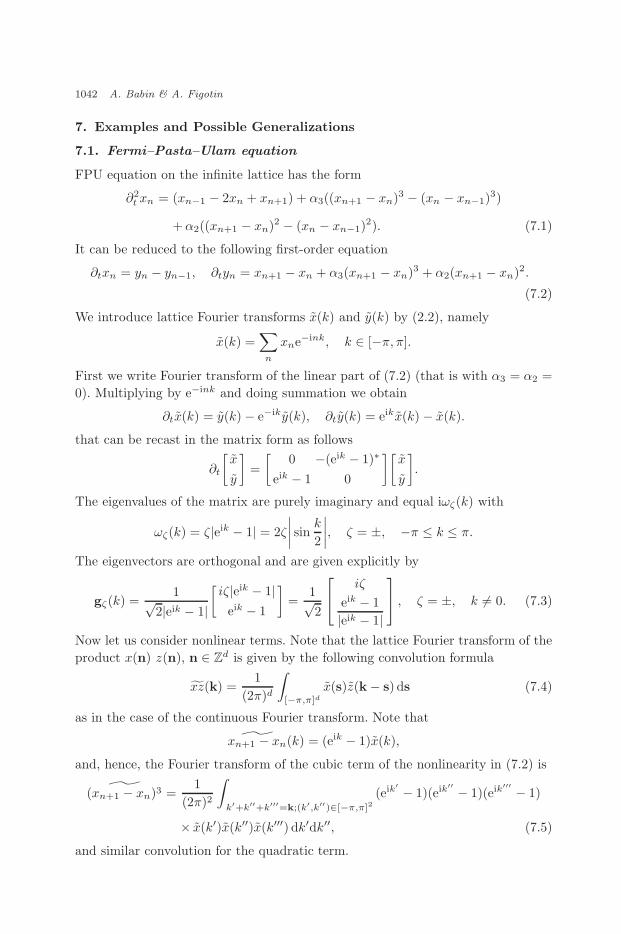
A particular example of (2.3) is obtained as a Fourier transform of the followingFermi–Pasta–Ulam equation (FPU) (see [12, 37, 44]) describing a nonlinear systemof coupled oscillators:

∂τxn =1�(yn − yn−1), (2.10)

∂τyn =1�(xn+1 − xn) + α2(xn+1 − xn)2 + α3(xn+1 − xn)3, n ∈ Z.

Note that an equivalent form of (2.10) (with α2 = 0) is the second-order equation

∂2τxn =

1�2

(xn−1 − 2xn + xn+1) +α3

�((xn+1 − xn)3 − (xn − xn−1)3). (2.11)

In this example d = 1, k = k and elementary computations show that the Fouriertransform of the FPU equation (2.10) has the form of the modal evolution equation(2.3), (2.9) where

U =[

x

y

], iL(k) =

[0 −(1 − e−ik)∗

(1 − e−ik) 0

], ωζ(k) = 2ζ

∣∣∣∣sin k

2

∣∣∣∣,χ(2)(k, k′, k′′)U1(k′)U2(k′′) = α2(1 − e−ik′

)(1 − e−ik′′)[

0x1(k′)x2(k′′)

],

(2.12)

and a similar formula for χ(3) (see (7.5)).Now let us consider the general multi-component vector case with J > 1 which

we refer to as J-band case for which the system (2.3) has 2J components, andinstead of (2.7) we assume that L(k) has eigenvalues and eigenvectors as follows:

L(k)gn,ζ(k) = ωn,ζ(k)gn,ζ(k), ωn,ζ(k) = ζωn(k), ζ = ±, n = 1, . . . , J,

(2.13)

where ωn(k) are real-valued, continuous for all k functions, and eigenvectorsgn,ζ(k) ∈ C2J have unit length in the standard Euclidean norm. We also supposethat the eigenvalues are numbered so that

ωn+1(k) ≥ ωn(k) ≥ 0, n = 1, . . . , J − 1, (2.14)

and we call n the band index. Note that the presence of ζ = ± reflects a symmetry ofthe system allowing it, in particular, to have real-valued solutions. Such a symmetryof dispersion relation ωn(k) occurs in photonic crystals and many other physicalproblems.

Note that (2.13) implies that the following symmetry relation hold:

ωn,−ζ(k) = −ωn,ζ(k), n = 1, . . . , J. (2.15)

We also always assume that the following inversion symmetry holds:

ωn,ζ(−k) = ωn,ζ(k). (2.16)

Remark 2.1. Assuming (2.15) and (2.16) we suppose that the dispersion relationsωζ(k) have the same symmetry properties as the dispersion relations of Maxwell



equations in periodic media, see [1–3, 5]. We would like to stress that these symmetryconditions are not imposed for technical reasons but because they are consequencesof fundamental symmetries of physical media. Such symmetries arise in many prob-lems including, for instance, the Fermi–Pasta–Ulam equation, or when L(k) origi-nates from a Hamiltonian H(p, q) = 1

2 (H1(p2)) + 12H2(q2). In the opposite case if

it is assumed that (2.15) and (2.16) never hold, the results of this paper hold andthe proofs, in fact, are simpler. The case with the symmetry is more difficult anddelicate because of a possibility of resonant nonlinear interactions.

There are values of k for which inequalities (2.14) turn into equalities, thesepoints require special treatment.

Definition 2.2 (Band-Crossing Points). We call k0 a band-crossing point ifωn+1(k0) = ωn(k0) for some n or ω1(k0) = 0 and denote the set of band-crossingpoints by σ.

Everywhere in this paper we assume that the following condition is satisfied.

Condition 2.3. The set σ of band-crossing points is a closed nowhere dense setin Rd with zero Lebesgue measure, the entries of the matrix L(k) are infinitelysmooth functions of k /∈ σ and ωn(k) are continuous functions of kfor all k and areinfinitely smooth when k /∈ σ.

Observe that for k /∈ σ all the eigenvalues of the matrix L(k) are different andthe corresponding eigenvectors gn,ζ(k) of L(k)can be locally defined as smoothfunctions of k /∈ σ as long as L(k) is smooth.

Remark 2.4. The band-crossing points are discussed in more details in [1, 2]. Herewe only note that generically the singular set σ is a manifold of the dimension d−2,see [1, 2]. A simple example of a band-crossing point is k = 0 in (2.12).

Since we do not assume the matrix L(k) to be Hermitian, we impose the follow-ing condition on its eigenfunctions which guarantees its uniform diagonalization.

Condition 2.5. We assume that the 2J × 2J matrix formed by the eigenvectorsgn,ζ(k) of L(k), namely,

Ξ(k) = [g1,+(k),g1,−(k), . . . ,gJ,+(k),gJ,+(k)]

is uniformly bounded together with its inverse

supk/∈σ

‖Ξ(k)‖, supk/∈σ

‖Ξ−1(k)‖ ≤ CΞ for some constant CΞ. (2.17)

Here and everywhere we use the standard Euclidean norm in C2J .

Note that if the matrix L(k) is Hermitian for every k, the eigenvectors forman orthonormal system. Then the matrix Ξ, which diagonalizes L, is unitary and(2.17) is satisfied with CΞ = 1. Everywhere throughout the paper we assume thatCondition 2.5 is satisfied.



We introduce for vectors u ∈ C2J their expansion with respect to the basis gn,ζ :

u(k) =J∑

n=1

∑ζ=±

un,ζ(k)gn,ζ(k) =J∑

n=1

∑ζ=±

un,ζ(k), (2.18)

and we refer to it as the modal decomposition of u(k), and call the coefficientsun,ζ(k) the modal coefficients of u(k). In this expansion we assign to every n, ζ alinear projection Πn,ζ(k) in C2J corresponding to gn,ζ(k), namely

Πn,ζ(k)u(k) = un,ζ(k)gn,ζ(k) = un,ζ(k), n = 1, . . . , J, ζ = ±. (2.19)

Note that these projections may be not orthogonal if L(k) is not Hermitian.Evidently the projections Πn,ζ(k) are determined by the matrix L(k) and there-fore do not depend on the choice of the basis gn,ζ(k). Projections Πn,ζ(k) dependsmoothly on k /∈ σ (note that we do not assume that the basis elements gn,ζ(k)are defined globally as smooth functions for all k /∈ σ, in fact band-crossing pointsmay be branching points for eigenfunctions, see, for example, [1].) They are alsouniformly bounded thanks to Condition 2.5:

C−1Ξ |V| ≤

(∑n,ζ

|Πn,ζ(k)V|2)1/2

≤ CΞ|V|, V ∈ C2J , k /∈ σ. (2.20)

We would like to point out that most of the quantities are defined outside of thesingular set σ of band-crossing points. It is sufficient since we consider U(k) as anelement of the space L1 of Lebesgue integrable functions and the set σ has zeroLebesgue measure.

The class of nonlinearities F in (2.3) which we consider can be described asfollows. F is a general polynomial nonlinearity of the form

F (U) =mF∑m=2

F (m)(Um), with mF ≥ 2, (2.21)

where m-linear operators F (m) are represented by integral convolution formulassimilar to (2.9), namely

F (m)(U1, . . . , Um)(k, τ) =∫

Dm

χ(m)(k, �k)U1(k′) · · · Um(k(m)(k, �k)) d(m−1)d�k,

(2.22)

where the domain

Dm = [−π, π](m−1)d, (2.23)

and we use notation

d(m−1)d�k =1

(2π)(m−1)ddk′ · · · dk(m−1) (2.24)

and

k(m)(k, �k) = k − k′ − · · · − k(m−1), �k = (k′, . . . ,k(m)). (2.25)



Condition 2.6 (Nonlinearity Regularity). The nonlinear operator F (U)defined by (2.21) satisfy

‖χ(m)‖ =1

(2π)(m−1)dsup

k,k′,...,k(m)‖χ(m)(k,k′, . . . ,k(m))‖ ≤ Cχ, m = 2, 3, . . . ,

(2.26)

where, without loss of generality, we can assume that Cχ ≥ 1. The norm |χ(m)(k, �k)|of the tensor χ(m) with a fixed �k as a m-linear operator from (C2J )m into (C2J) isdefined by

|χ(m)(k, �k)| = sup|xj |≤1

|χ(m)(k, �k)(x1, . . . ,xm)|, (2.27)

where as always, | · | stands for the standard Euclidean norm. The tensors χ(m)(k, �k)are assumed to be smooth functions of k,k′, . . . ,k(m) /∈ σ, namely for every com-pact K ⊂ Rd\σ and for all m = 2, 3, . . .

|∇lχ(m)(k,k′, . . . ,k(m))| ≤ CK,l if k,k′, . . . ,k(m) ∈ K, l = 1, 2, . . . , (2.28)

where ∇lχ(m) is the vector composed of all partial derivatives of order l of allcomponents of the tensor χ(m) with respect to the variables k,k′, . . . ,k(m).

From now on all the nonlinear operators we consider are assumed to satisfy thenonlinearity regularity Condition 2.6.

Remark 2.7. At first sight, since � is a small parameter, one might think that thelinear term in (2.1) with the factor 1

� is dominant. But it is not that simple. Indeed,

since all eigenvalues of L(k) are purely imaginary the magnitude of e−i� L(k)h(k)

which represents the solution of a linear equation (with F = 0) is bounded uniformlyin �. A nonlinearity F alters the solution for a bounded time τ∗ which is not smallfor small �. Therefore the influence of the nonlinearity can be significant. Thisphenomenon can be illustrated by the following toy model. Let us consider thepartial differential equation for a scalar function y(x, τ):

∂τy = −1�∂xy + y2, y(x, 0) = h(x).

Its solution is of the form

y(x, τ) =h

(x − τ

�

)1 − τh

(x − τ

�

) , (2.29)

and regularly it exists only for a finite time. The solution (2.29) shows that thelarge coefficient 1

� enters it so that the corresponding wave moves faster with thevelocity 1

� along the x-axis but the wave’s shape does not depend on � at all. For

the NLS with the initial data h(k) = h(k, β), � = β2, and the coefficient 1� at the



linear part, the nonlinearity balances the effect of dispersion leading to emergenceof solitons, see [6] for a discussion.

To formulate our results we introduce a Banach space E = C([0, τ∗], L1) offunctions v(k, τ), 0 ≤ τ ≤ τ∗, with the norm

‖v(k, τ)‖E = ‖v(k, τ)‖C([0,τ∗],L1) = sup0≤τ≤τ∗

∫[−π,π]d

|v(k, τ)| dk. (2.30)

Here L1 is the Lebesgue function space with the standard norm defined by theformula

‖v(·)‖L1 =∫

[−π,π]d|v(k)| dk. (2.31)

The following theorem guarantees the existence and the uniqueness of a solution tothe modal evolution equation (2.3) on a time interval which does not depend on �

(see Theorem 5.4 for details).

Theorem 2.8 (Existence and Uniqueness). Let the model evolution equation(2.3) satisfy the Condition 2.5, and let h ∈ L1, ‖h‖L1 ≤ R. Then there exists aunique solution U = G(h) of (2.3) which belongs to C1([0, τ∗], L1). The numberτ∗ > 0 depends on R, Cχ and CΞ and it does not depend on �.

Now we would like to formulate the main result of this paper, a theorem onthe superposition principle, showing that the generic wavepackets evolve almostindependently for the case of lattice equations. To do that, first, we define animportant concept of wavepacket.

Definition 2.9 (Wavepacket). A function h(β,k) which depends on a parameter0 < β < 1, is called a wavepacket with a center k∗ if it satisfies the followingconditions:

(i) It is bounded in L1 uniformly in β, i.e.

‖h(β, ·)‖L1 ≤ Ch. (2.32)

(ii) It is composed of modes from essentially a single band n, namely for any0 < ε < 1 there is a constant Cε > 0 such that

‖h(k) − h−(k) − h+(k)‖L1 ≤ Cεβ, hζ(k) = Πn,ζh(k), ζ = ±, (2.33)

and hζ(β,k) is essentially supported in a small vicinity of ζk∗, where k∗ is thewavepacket center, namely∫

|k−ζk∗|≥β1−ε

|hζ(β,k)| dk ≤ Cεβ. (2.34)

(iii) The wavepacket center k∗ is not a band-crossing point, that is k∗l /∈ σ, andthe following regularity condition holds:∫

|k−ζk∗|≤β1−ε

|∇khζ(β,k)| dk ≤ Cεβ−1−ε. (2.35)

In the above conditions (ii) and (iii), Cε does not depend on β, 0 < β < 1.



The simplest example of a wavepacket in the sense of Definition 2.9 is a functionof the form

hζ(β,k) = β−dhζ

(k − ζk∗

β

)gn,ζ(k), ζ = ±, (2.36)

where hζ(k) is a Schwartz function, that is an infinitely smooth, rapidly decayingfunction. Another typical and natural example of a wavepacket h centered at k∗ isreadily provided by

h(β,k) = Πn,+(k)h0,+(β,k) + Πn,−(k)h0,−(β,k), (2.37)

where h0,ζ(β,k) is the lattice Fourier transform of the following function

h0,ζ(m, β) = eiζk∗·mΦζ(βm − r0)g, ζ = ±, (2.38)

where g is a vector in C2J , projection Πn,ζ is as in (2.19) with some n, vectorsm, r0 ∈ Rd and Φζ(r) being an arbitrary Schwartz function (see Lemma 7.2).

Our special interest is in the waves that are finite sums of wavepackets and werefer to them as multi-wavepackets.

Definition 2.10 (Multi-Wavepacket). A function h(β,k), 0 < β < 1, is calleda multi-wavepacket if it is a finite sum of wavepackets hl as defined in Definition 2.9,namely

h(β,k) =Nh∑l=1

hl(β,k), (2.39)

and we call the set {k∗l} of all the centers k∗l of involved wavepackets center set of h.

In what follows we will be interested in generic multi-wavepackets such that theircenters are generic. The exact meaning of this is provided below in the followingconditions.

Condition 2.11 (Non-Zero Frequency). We assume that every center k∗l of awavepacket satisfies the following condition

ωnl(k∗l) = 0, l = 1, . . . , Nh. (2.40)

Condition 2.12 (Group Velocity). We assume that all centers k∗l, l =1, . . . , Nh, of the multi-wavepacket h as defined in Definition 2.10 are not band-crossing points, and the gradients ∇kωnlj

(k∗lj ) (called group velocities) at thesepoints satisfy the following condition

|∇kωnl1(k∗l1) −∇kωnl2

(k∗l2 )| = 0 when l1 = l2, (2.41)

indicating that the group velocities are different.

We also want the functions (dispersion relations) ωnl(k) to be non-degenerate

in the sense that they are not exactly linear, below we give exact conditions.



Consider the following equation for n and θ

θωnl(k∗) − ζωn(θk∗) = 0, ζ = ±1, (2.42)

where the admissible θ have the form

θ =m∑

j=1

ζ(j), ζ(j) = ±1, m ≤ mF , (2.43)

mF is the same as in (2.21). In the case when in the series (2.21) some terms F (m)

vanish, we take in (2.43) only m corresponding to non-zero F (m).

Condition 2.13 (Non-Degeneracy). Given a point k∗ = k∗l and band nl weassume that dispersion relations ωn(k) are such that all solutions n, θ of (2.42) arenecessarily of the form

n = nl, θ = ζ. (2.44)

Definition 2.14 (Generic Multi-Wavepackets). A multi-wavepacket h asdefined in Definition 2.10 is called generic if the centers k∗l, l = 1, . . . , Nh, of allwavepackets satisfy Conditions 2.11 and 2.12; and the dispersion relations ωn(k) atevery k∗l and band nl satisfy Condition 2.13.

We introduce now the solution operator G mapping the initial data h into thesolution U = G(h) of the modal evolution equation (2.3); this operator is definedfor ‖h‖ ≤ R according to Theorem 2.8. The main result of this paper for the latticecase is the following statement.

Theorem 2.15 (Superposition Principle for Lattice Equations). Supposethat the initial data h of (2.3) is a multi-wavepacket of the form

h =Nh∑l=1

hl, Nh maxl

‖hl‖L1 ≤ R, (2.45)

satisfying Definition 2.10, where h is generic in the sense of Definition 2.14. Let usassume that

β2

�≤ C, with some C, 0 < β ≤ 1

2, 0 < � ≤ 1

2. (2.46)

Then the solution U = G(h) to the evolution equation (2.3) satisfies the followingapproximate superposition principle

G(

Nh∑l=1

hl

)=

Nh∑l=1

G(hl) + D, (2.47)

with a small remainder D(τ) satisfying the following estimate

sup0≤τ≤τ∗

‖D(τ)‖L1 ≤ Cε�

β1+ε|ln β|, (2.48)

where ε is the same as in Definition 2.9 and can be arbitrary small, τ∗ does notdepend on β, � and ε.



The most common case when (2.46) holds is � = β2, a discussion of differentscalings is provided in [6, 7].

Observe that solutions to the original evolution equation (2.1) with the initialdata (2.39), (2.38) satisfy the superposition principle if the wave vectors k∗l in(2.38) satisfy (2.41), (2.42) and Φl are Schwartz functions. It turns out, that theevolution of every coefficient un,ζ(k) of the solution as defined by (2.18) can beaccurately approximated by a solution a relevant nonlinear Schrodinger equation(NLS), see [23]. Therefore Theorem 2.15 provides a reduction of multi-wavepacketproblem to several single-wavepacket problems.

We also would like to stress that though β is small the nonlinear effects are notsmall. Namely, there can be a significant difference between solutions of a nonlinearand the corresponding linear (with F (U) being set zero) equations with the sameinitial data for times τ = τ∗.

Recall that up to now we analyzed the nonlinear evolution in the modal form(2.3) for U(k, τ). To make a statement on the nonlinear evolution for the origi-nal evolution equation (2.1), i.e. in terms of the quantities U(m, τ), we introduceU(h)(m) as the inverse Fourier transform of the solution G(h)(k) of the modalevolution equation (2.3). Recall that the inverse Fourier transform correspondingto (2.2) is given by the formula

U(m) = (2π)−d

∫[−π,π]d

eim·kU(k) dk, (2.49)

and when applying the inverse Fourier transform we get back the original latticesystem (2.1) from its modal form (2.3). The convolution form of the nonlinearitymakes the lattice system invariant with respect to translations on the lattice Zd.Using Theorem 2.15 and applying the inverse Fourier transform together with theinequality

‖U‖L∞ ≤ (2π)−d‖U‖L1 (2.50)

we obtain the following statement.

Corollary 2.16. Let the evolution equation (2.1) be obtained as the lattice Fouriertransform of (2.3). If h is given by (2.38) where every Φl,ζ(r) is a Schwartz function(that is an infinitely smooth, rapidly decaying function) then U(h) is a solution tothe evolution equation (2.1). If h = h1 + · · · + hNh

and every hl is given by (2.38)then the approximate superposition principle holds:

U(h) = U(h1) + · · · + U(hNh) + D, (2.51)

with a small coupling remainder D(τ) satisfying

sup0≤τ≤τ∗

‖D(τ)‖L∞ ≤ C′δ

�

β1+δ, (2.52)

where δ > 0 can be taken arbitrary small.



As an application of Theorem 2.15 let us consider the Fermi–Pasta–Ulam equa-tion (2.10). We impose the initial condition for (2.10)

xn(0) =nh∑l=1

Ψ0l(βn − rl)eik∗ln + cc,

(2.53)

yn(0) =nh∑l=1

Ψ1l(βn − rl)eik∗ln + cc, n ∈ Z,

where Ψ0l(r), Ψ1l(r) are arbitrary Schwartz functions, and rl are arbitrary realnumbers, cc means complex conjugate to the preceding terms and assume that �, β

satisfy (2.46). For any given k∗l there are two eigenvectors g±(k∗l) of the matrixL(k∗l) in (2.12) given by (7.3) and corresponding terms in (2.53) can be written as[

Ψ0l

Ψ1l

]eik∗ln = [Φ−,lg−(k∗l) + Φ+,lg+(k∗l)]eik∗ln.

In this case all requirements of Definition 2.10 are fulfilled, and (2.53) definesa multi-wavepacket. Note that the multi-wavepacket (2.53) involves Nh = 2nh

wavepackets with 2nh wavepacket centers ϑk∗l, ϑ = ±. To satisfy Condition 2.12the wavepacket centers k∗l must satisfy

cosk∗l

2∣∣∣∣sin k∗l

2

∣∣∣∣ =cos

k∗j

2∣∣∣∣sin k∗j

2

∣∣∣∣ if l = j. (2.54)

To check if the centers k∗l satisfy Condition 2.13 we consider the equation

z

∣∣∣∣sin k∗l

2

∣∣∣∣− ζ

∣∣∣∣sin(zk∗l

2

)∣∣∣∣ = 0, z =3∑

j=1

ζ(j), ζ(j) = ±1. (2.55)

Evidently the possible values of z are −3,−1, 1, 3. Since the equation 3|sin φ| =|sin(3φ)| has the only solution φ = 0 on [0, π/2], Eq. (2.55) has the only solutionz = ζ. Consequently, all points k∗l = 0 satisfy Condition 2.13, and Theorem 2.15applies. The initial data for a single wavepacket solution have the form[

xϑ,n,l(0)yϑ,n,l(0)

]= Φϑ,l(βn − rl)gϑ(k∗l) + cc, n ∈ Z, ϑ = ±. (2.56)

According to this theorem and Corollary 2.16 the solution to (2.10), (2.53) equalsthe sum of solutions of (2.10) with single wavepacket initial data, that is

xn(τ) =∑ϑ=±

nh∑l=1

xϑ,n,l(τ) + D1,n(τ), yn(τ) =∑ϑ=±

nh∑l=1

yϑ,n,l(τ) + D2,n(τ),

(2.57)



y

3

2

1

0

-1

-2

-3

x

40200-20-40

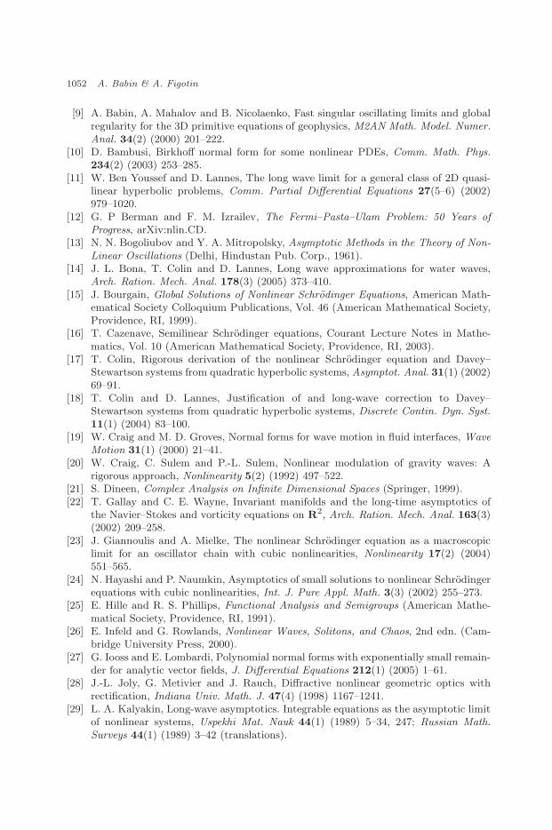
Fig. 1. In this picture, two wavepackets are shown with different “centers” k∗1 and k∗2. The val-ues of k∗1 and k∗2 are proportional to the frequences of spatial oscillations. Though the wavepack-ets overlap in physical space, they pass one through another in the process of nonlinear evolutionalmost without interaction if their group velocities are different.

where Dn is a small remainder satisfying

sup0≤τ≤τ∗

supn

[|D1,n(τ)| + |D2,n(τ)|] ≤ Cδ�

β1+δ(2.58)

with arbitrarily small positive δ. Hence, the following statement holds.

Theorem 2.17 (Superposition for Fermi–Pasta–Ulam Equation). If everyΦl,ζ(r) is a Schwartz function, and the wavevectors k∗l = 0 satisfy (2.54), then thesolution xn(τ), yn(τ) of the initial value problem for the Fermi–Pasta–Ulam equa-tion (2.10) with multi-wavepacket initial condition (2.53) is a linear superpositionof solutions xn,l(τ), yn,l(τ) of the same equation with single-wavepacket initial con-dition (2.56) up to a small coupling term D1,n(τ), D2,n(τ) satisfying (2.57), (2.58)with arbitrary small δ > 0 and τ∗ which do not depend on β, �, δ.

Note that solutions xϑ,n,l(τ) with different ϑ, l resemble 2nh solitons which orig-inate at different points rl and propagate with different group velocities. Accordingto (2.57), (2.58) all these soliton-like wavepackets pass through one another with verylittle interaction, see Fig. 1. Note that Theorem 2.15 shows that this phenomenon isrobust in the class of general difference equations on the lattice Z, and that it per-sists under polynomial perturbations of the nonlinearity as well as perturbations ofthe linear part of Eq. (2.11) as long as they leave the linear difference operator non-positive and self-adjoint. Observe also that the evolution of every single wavepacketis nonlinear, and it is well-approximated by a properly constructed NLS (we intendto write a proof of this statement for general lattice systems in another article;see [23] for a particular case). For example, for a special choice of Ψjl the solutionxn,l(τ) can be well-approximated by a soliton solution of a corresponding NLS.



2.2. Main statements and examples for semilinear systems

of hyperbolic PDE

In this subsection, we consider nonlinear evolution equation involving partial differ-ential (and pseudodifferential) operators with respect to spatial variables with con-stant coefficients in the entire space Rd. There is a great deal of similarity betweensuch nonlinear evolution PDE and the lattice nonlinear evolution equations con-sidered in the previous section. In particular, we study first not the original PDEbut its Fourier transform, modal evolution equation, and the results concerning theoriginal PDE are obtained by applying the inverse Fourier transform.

Recall that for functions U(r) from L1(Rd) the Fourier transform and its inverseare defined by the formulas

U(k) =∫

Rd

U(r)e−ir·k dr, where k ∈ Rd, (2.59)

U(r) =1

(2π)d

∫Rd

U(k)eir·k dr, where r ∈ Rd. (2.60)

Similarly to (2.3) we introduce the following modal evolution equation

∂τ U(k, τ) = − i�L(k)U(k, τ) + F (U)(k, τ), U(k, 0) = h(k), k ∈ Rd, (2.61)

where (i) U(k, τ) is a 2J-component vector-function of k, τ , (ii) L(k) is a 2J × 2J

matrix function of k, and (iii) F (U) is the nonlinearity. We assume that the 2J×2J

matrix L(k), k ∈ Rd, has exactly 2J eigenvectors gn,ζ(k) with corresponding2J real eigenvalues ωn,ζ(k) satisfying the relations (2.13)–(2.17). We also assumethe matrix L(k), k ∈ Rd, to satisfy the polynomial bound

|L(k)| ≤ C(1 + |k|p). (2.62)

The singular set σ for L(k) is as in Definition 2.3 with the only difference that func-tions ωn,ζ(k) are defined over Rd rather than the torus [−π, π]d, and, consequentlythey are not periodic. The nonlinearity F (U) has a form entirely similar to (2.21):

F (U) =mF∑m=2

F (m)(Um), (2.63)

with F (m) being m-linear operators with the following representation similarto (2.22):

F (m)(U1, . . . , Um)(k)

=∫

Dm

χ(m)(k, �k)U1(k′) · · · Um(k(m)(k, �k)) d(m−1)d�k, (2.64)



where k(m)(k, �k) is defined by the convolution equation (2.25), d is defined by (2.24)and Dm in (2.64) is now defined not by (2.23) but by

Dm = R(m−1)d. (2.65)

The difference with (2.3) now is that the involved functions of k, k′ etc. are not2π-periodic, Dm in (2.64) is defined by (2.65) instead of (2.23), and the tensorsχ(m)(k, �k) satisfy the nonlinear regularity Condition 2.6 without the periodicityassumption. The functions Ul(k(l)) in (2.64) are assumed to be from the spaceL1 = L1(Rd) with the norm

‖U(·)‖L1 =∫

Rd

|v(k)| dk. (2.66)

We seek solutions to (2.61) in the space C1([0, τ∗], L1) with 0 < τ∗ ≤ 1.Applying the inverse Fourier transform to the modal evolution equation (2.61)

we obtain a hyperbolic 2J-component systems in Rd of the form

∂τU(r, τ) = − i�L(−i∇r)U(r, τ) + F (U)(r, τ), U(r, 0) = h(r). (2.67)

Note that since L(k) satisfies the polynomial bound (2.62) we can define the actionof the operator L(−i∇r) on any Schwartz function Y(r) by the formula

L(−i∇r)Y(k) = L(k)Y(k), (2.68)

where, in view of (2.62), the order of L does not exceed p. If all the entries of L(k)are polynomials, such a definition coincides with the common definition of theaction of a differential operator L(−i∇r). In this case L(−i∇r) defined by (2.68) isa differential operator with constant coefficients of order not greater than p.

The properties of the modal evolution equation (2.61) are completely similar toits lattice counterpart and are as follows. The existence and uniqueness theorem issimilar to Theorem 2.8.

Theorem 2.18 (Existence and Uniqueness). Let Eq. (2.61) satisfy conditions(2.17) and (2.26) and h ∈ L1 = L1(Rd), ‖h‖L1 ≤ R. Then there exists a uniquesolution to the modal evolution equation (2.61) in the functional space C1([0, τ∗], L1).The number τ∗ depends on R, Cχ and CΞ.

Here is the main result for the semilinear hyperbolic systems of PDE which iscompletely similar to Theorem 2.15.

Theorem 2.19 (Principle of Superposition for PDE Systems). Let the ini-tial data of the modal evolution equation (2.61) be a multi-wavepacket, i.e. the sumof Nh wavepackets hl as in (2.45) satisfying Definitions 2.9 and 2.10. Supposethat �, β satisfy condition (2.46). Assume also that h is generic in the sense of



Definition 2.14. Then the solution U = G(h) to the modal evolution equation (2.61)satisfies the approximate linear superposition principle, namely

G(

Nh∑l=1

hl

)=

Nh∑l=1

G(hl) + D, (2.69)

with a small remainder D(τ)

sup0≤τ≤τ∗

‖D(τ)‖L1 ≤ Cε�

β1+ε|ln β|, (2.70)

where ε is the same as in Definition 2.9, τ∗ does not depend on β, � and ε. The solu-tions U(h)(r, τ) of the space evolution equation (2.67) are obtained as the inverseFourier transform of G(h) and they satisfy the approximate linear superpositionprinciple, namely

U(h) = U(h1) + · · · + U(hNh) + D, (2.71)

with a small coupling remainder D(τ) satisfying

sup0≤τ≤τ∗

‖D(τ)‖L∞ ≤ Cε�

β1+ε|ln β|, (2.72)

where ε > 0 is the same as in Definition 2.9 and can be arbitrary small.

Example 1. Sine-Gordon and Klein–Gordon Equations with Small InitialData. Let us consider the sine-Gordon equation (see [26])

∂2t u = ∂2

ru − sinu (2.73)

with small initial data

u(r, 0) = βb0, ∂tu(r, 0) = βb1, β � 1. (2.74)

First, we recast this the equation into our framework by rescaling the variables

u = βU1, β2t = τ. (2.75)

Since sinβU1 = βU1− 16β3U3

1 +β5f(U1), where evidently f(U1) is an enitire function,we can recast Eq. (2.73) into the following form

∂2τU1 =

1β4

[∂2xU1 − U1] +

1β2

[qU31 + β2f(U1)]. (2.76)

We introduce then a linear pseudodifferential operator A = (I − ∂2x)1/2 with the

symbol (1 + k2)1/2 and rewrite Eq. (2.76) as the following system

∂τU1 =1β2

AU2, ∂τU2 = − 1β2

AU1 + A−1[qU31 + β2f(U1)], (2.77)

with the initial data

U1(0) = h0, U2(0) = h1, (2.78)



where h0 and h1 are assumed to be of the form

z(r, 0) = h0, p(r, 0) = h1, hj =nh∑l=1

Ψjl(βr − rl)eik∗l·r + cc, j = 0, 1,

(2.79)

in one-dimensional case with r = r, k = k. Evidently, the relations with the initialdata of (2.73) are

b0 = h0, b1 = Ah1.

Notice that the system (2.77) is of the form (2.67) with

� = β2, LU =[

AU2

−AU1

], F (U) = F0(U) + β2F1(U), (2.80)

F0(U) = A−1

[0

qU31

], F1(U) = A−1

[0

f(U1)

].

Observe now that L has only one spectral band with the dispersion relation andeigenvectors given by

ω(k) = (I + k2)1/2, gϑ(k) = gϑ = 2−1/2

[−iϑ1

], ϑ = ±1,

and there is no band-crossing points. We use expansion in the basis g±[Ψ0l

Ψ1l

]eik∗l·r = [Φ+,lg+ + Φ−,lg−]eik∗l·r (2.81)

to represent initial data (2.78) and (2.79). Here Eq. (2.42) takes the form

(1 + k2∗l)

1/2λ = ζ(1 + λ2k2∗l)

1/2, ζ = ±1.

Obviously, this equation has only solutions λ = ζ and Condition 2.13 is fulfilled.Condition 2.12 holds if

ϑk∗l

(1 + k2∗l)1/2

= ϑ′k∗l′

(1 + k2∗l′ )1/2

for l = l′ or ϑ = ϑ′ (2.82)

which is equivalent to

k∗l′ = k∗l for l′ = l, and k∗l = 0 for all l. (2.83)

Equation (2.77) can be written in the integral form (3.3) with mF = ∞ and byTheorem 5.4, it has unique solution U for τ ≤ τ∗. If we replace F (U) in (2.80) byF0(U), we obtain

∂τV1 =1β2

AV2, ∂τV2 = − 1β2

AV1 + A−1qV 31 , (2.84)

where we take the initial data to be as in (2.78), namely

V1(0) = h0, V2(0) = h1. (2.85)

Equations (2.84) can be obtained by replacing sinu in (2.73) by the cubic polyno-mial u−u3/6 producing the quasilinear Klein–Gordon equation (see [36]). Observe



that the solutions to the sine-Gordon and the Klein–Gordon equations with smallinitial data are very close. To see that, note that the operator f(U)(k) is boundedin L1 for U(k) which are bounded in L1. Therefore the norm of the neglected termis small, namely ‖β2f(U)‖L1 ≤ Cβ2. Thus, by Remark 4.8, the solutions of (2.77)and (2.84) are close, namely

‖U1 − V1‖L∞ + ‖U2 − V2‖L∞ ≤ Cβ2, 0 ≤ τ ≤ τ∗. (2.86)

According to Theorem 2.19 the superposition principle is applicable to Eq. (2.84)with initial data as in (2.85), and the following statements hold.

Theorem 2.20 (Superposition for Klein–Gordon). Assume that the initialdata h0, h1 in (2.85) are as in (2.79). Then the solution {V1, V2} to the system(2.84) satisfies the linear superposition principle, namely

V1(r, τ) =∑ϑ=±

nh∑l=1

V1,ϑ,l(r, τ) + D1(r, τ),

V2(r, τ) =∑ϑ=±

nh∑l=1

V2,ϑ,l(r, τ) + D2(r, τ),

(2.87)

where {V1,ϑ,l(r, τ), V2,ϑ,l(r, τ)} is a solution to (2.84) with the one-wavepacket initialcondition [

V1,ϑ,l(r, 0)V2,ϑ,l(r, 0)

]= Φϑ,l(βr − rl)gϑeik∗l·r + cc, (2.88)

where Φϑ,l(r) are arbitrary Schwartz functions. If (2.83) holds, the coupling termsD1,D2 satisfy the bound

sup0≤τ≤τ∗

[‖D1(τ)‖L∞ + ‖D2(τ)‖L∞ ] ≤ C′δ

�

β1+δ= C′

δβ1−δ, (2.89)

where τ∗ and C′δ do not depend on β, and δ can be taken arbitrary small.

Using (2.86) we obtain a similar superposition theorem for the sine-Gordonequation.

Theorem 2.21 (Superposition for Sine-Gordon). Assume that the initial datah0, h1 in (2.78) are as in (2.79). Then the solution {U1, U2} to (2.77), (2.78) satisfiesthe linear superposition principle, namely

U1(r, τ) =∑ϑ=±

nh∑l=1

U1,ϑ,l(r, τ) + D1(r, τ),

U2(r, τ) =∑ϑ=±

nh∑l=1

U2,ϑ,l(r, τ) + D2(r, τ),



where U1,ϑ,l(r, τ), U2,ϑ,l(r, τ) is a solution of (2.77) with the one-wavepacket initialcondition [

U1,ϑ,l(r, 0)U2,ϑ,l(r, 0)

]= Φϑ,l(βr − rl)gϑeik∗l·r + cc, ϑ = ±,

where Φϑ,l(r) are arbitrary Schwartz functions. If (2.83) holds, the coupling termsD1,D2 satisfy the bound (2.89).

Note that a theorem completely similar to Theorem 2.20 holds also for a gen-eralized Klein–Gordon equation where qV 3

1 is replaced by an arbitrary polynomialP (V1). Hence, the superposition principle holds for the sine-Gordon equation (2.73)with a small initial data and a strongly perturbed nonlinearity as, for example, whensin u is replaced by sin u + β−1u4 + β−2u5.

We would like to compare now our results and methods with that of [38] wherethe interaction of counterpropagating waves is studied by the ansatz method. Pierceand Wayne considered in [38] the sine-Gordon equation in the case of small initialdata which have the form of a bimodal wavepacket. In our notation it correspondsto the case when � = β2, nh = 1 in (2.79), when two wavepackets, correspondingto ϑ = + and ϑ = −, have exactly opposite group velocities. They proved that thebimodal wavepacket data generate two waves which are described by two uncouplednonlinear Schrodinger equations with a small error. The magnitude of the errorgiven in [38] (which we formulate here for the solution U1 of the rescaled equation(2.76)) is estimated by Cβ1/2 on the time interval 0 ≤ τ ≤ τ0 (or 0 ≤ t ≤ τ0β

−2).Note that our general Theorem 2.19 when applied to the special case of the sine-Gordon equation (2.76) provides a better estimate of the coupling error, namelyC�/β1+δ = Cβ1−δ in (2.89) with arbitrary small δ, for the same time interval.Notice that the estimate (2.72) given in Theorem 2.19 is almost optimal, since it ispossible to construct examples when the coupling error is greater than cβ1+δ witharbitrary small δ.

We would like to point out that the general mechanism responsible for thewavepacket decoupling is the destructive wave interference, this mechanism is subtlethough general. We treat the destructive wave interference by taking into accountexplicitly all nonlinear interactions of high-frequency waves. In our approach, we usethe exact representation of a general solution in the form of a functional-analyticoperator monomial series, every term of the series is explicitly given as a multilinearoscillatory integral operator applied to the initial data. A key advantage of such anapproach is that it allows to estimate wavepacket coupling as a sum of contributionsof highly oscillatory terms and to get a precise estimate of magnitude of everyterm. In contrast, the well-known “ansatz” approach as, for instance, in [38, 32],requires to find a clever ansatz with consequent estimations of the “residuum” in anappropriate norm. Our approach can naturally treat general tensorial polynomialnonlinearities F of arbitrary large degree NF and any number of wavepackets,whereas finding a good ansatz which allows to estimate the residuum in such a



general situation would be difficult. For readers interested in detailed features ofone-wavepacket solutions to the sine-Gordon equations, we refer to [32, 38, 39].

Example 2. Nonlinear Schrodinger Equation. The nonlinear Schrodingerequation (NLS) with d spatial variables [42, 16, 15] has the form

∂τz(r, τ) = i1�γ(−i∇)z(r, τ) + α|z|2z(r, τ), z(r, 0) = h(r), r ∈ Rd, (2.90)

where α is a complex constant, γ(−i∇) is a second-order differential operator, itssymbol γ(k) is a real, symmetric quadratic form

γ(k) = γ(k,k) =∑

γijkikj , γ(−i∇)z = −∑

γij∂ri∂rj z.

To put the NLS into the framework of this paper, we introduce the following two-component system

∂τz+(r, τ) = i1�γ(−i∇)z+(r, τ) + αz−z2

+(r, τ),

∂τz−(r, τ) = −i1�γ(i∇)z−(r, τ) + α∗z+z2

−(r, τ), (2.91)

z+(r, 0) = h(r), z−(r, 0) = h∗(r), r ∈ Rd,

where α∗ denotes complex conjugate to α. Obviously if z(r, τ) is a solution of(2.90) then z+(r, τ) = z(r, τ), z−(r, τ) = z∗(r, τ) gives a solution of (2.91). Usingthe Fourier transform we get from (2.90)

∂τ z(k, τ) = i1�γ(k)z(k, τ) + α(z∗z2)(k, τ), k ∈ Rd. (2.92)

Now the band-crossing set σ = {k ∈ Rd : γ(k) = 0}. We assume that the quadraticform γ is not identically zero. The Fourier transform of (2.91) takes the form of(2.67) with

U =[

U+

U−

], L(k)U =

[γ(k) 0

0 −γ(−k)

][U+

U−

],

ω(k) = |γ(k)|, F (3)(U3) =

[α (z+(U)z+(U)z−(U))

α∗ (z−(U)z−(U)z+(U))

].

To satisfy the requirements of Condition 2.14 we have to take the wave vectorsk∗l /∈ σ so that

∇|γ(k∗l)| =2γ(k∗l)|γ(k∗l)|

γ(k∗l, ·) =2γ(k∗l′)|γ(k∗l′ )|

γ(k∗l′ , ·) if l = l′, (2.93)

which provides (2.41). Since

|γ(k∗l)|λ − ζ|γ(λk∗l)| = |γ(k∗l)|[λ − ζ|λ|2],



and λ is odd, every point k∗l /∈ σ satisfies Condition 2.13. If the quadratic form γ

is not singular, that is det γ = 0, then condition (2.93), which ensures that groupvelocities of wavepackets are different, holds when

γ(k∗l)|γ(k∗l)|

k∗l =γ(k∗l′)|γ(k∗l′)|

k∗l′ if l = l′.

In this case Theorem 2.19 is applicable, and generic wavepacket solutions of the NLSare linearly superposed and propagate almost independently with coupling O(β).More precisely, as a corollary of Theorem 2.19 we obtain the following statement.

Theorem 2.22 (Superposition for NLS). Assume that initial data of the NLS(2.90) have the form h = h1 + · · · + hNh

,

hl(r) = eik∗l·mΦl,+(βr − r0) + e−ik∗l·mΦl,−(βr − r0), l = 1, . . . , Nh,

where Φl,ζ(r) are arbitrary Schwartz functions. Assume also that det γ = 0 and thevectors k∗l satisfy conditions

γ(k∗l) = 0, l = 1, . . . , Nh; k∗l = k∗l′ if l = l′.

Then solution z = z(h) is a linear superposition

z(h) = z(h1) + · · · + z(hNh) + D

with a small coupling term D

sup0≤τ≤τ∗

‖D(τ)‖L∞(Rd) ≤ Cδ�

β1+δ,

where δ > 0 can be taken arbitrary small.

We note in conclusion, that the superposition principle reduces dynamics ofmulti-wavepacket solutions to dynamics of single-wavepacket solutions; we do notstudy dynamics of single-wavepacket solutions in this paper. Note that the theory ofNLS-type approximations of one-wavepacket solutions of hyperbolic PDE is well-developed, see [29, 30, 18, 40, 41, 5] and references therein. Relevance of differentgroup velocities of wavepackets for smallness of their interaction was noted in [29].

2.3. Generalizations

Note that in a degenerate case when the function ωnl(k) is linear in the direction

of k∗, Eq. (2.42) for ζ = 1 has many solutions for which θ = ±1 and Condition 2.13does not hold. It turns out, that if Condition 2.13 for dispersion relations ωn(k)at k∗ is not satisfied, still we can prove our results under the following alternativecondition. We consider here the case of PDE in the entire space Rd and k ∈ Rd.



Condition 2.23 (Complete Degeneracy). The series (2.21) has only F (m) withodd m. The wavevectors k∗l and functions ωnl

(k), l = 1, . . . , Nh, have the followingthree properties:

(i) There exists δ > 0 such that for every l1 = l2, the following inequality holds:

|∇kωnl1(ν1k∗l1) −∇kωnl2

(ν2k∗l2)| ≥ δ, (2.94)

for any odd integers ν1, ν2 = 1, 3, . . . .

(ii) There exists δ > 0 such that νk∗l does not get in a δ-neighborhood of σ forany odd integer ν and any l = 1, . . . , Nh.

(iii) For any positive integer odd number θ and any k∗l, for any n the followingidentities hold:

∇kωn(θk∗l) = ∇kωn(k∗l), (2.95)

ωn(θk∗l) = θωn(k∗l). (2.96)

A nontrivial examples, where the above Condition 2.23 is satisfied, is givenbelow.

We give here a generalization of Definition 2.14.

Definition 2.24 (Generic Multi-Wavepackets). A multi-wavepacket h asdefined in Definition 2.10 is called generic if (i) the centers k∗l, l = 1, . . . , Nh, ofall wavepackets satisfy Conditions 2.11 and 2.12; (ii) either the dispersion relationsωn(k) at every k∗l and band nl satisfy Condition 2.13 or they satisfy Condition 2.23.

The statement of Theorem 2.19 remains true if Condition 2.14 is replaced byless restrictive Condition 2.24, namely the following theorem holds.

Theorem 2.25. Let the initial data of the modal evolution equation (2.61) be amulti-wavepacket, i.e. the sum of Nh wavepackets hl as in (2.45) satisfying Def-initions 2.9 and 2.10. Suppose that (2.46) holds. Assume also that h is genericin the sense of Definition 2.24. Then the solution U = G(h) to the modal evolu-tion equation (2.61) satisfies the approximate linear superposition principle, namely(2.69)–(2.72) hold.

The proofs we give in this paper directly apply to more general Theorem 2.25.Another generalization concerns the possibility to shift independently initial

wavepackets. If initial data involve parameters rl as in (2.79) it is possible to provethat Cε in (2.48), (2.70) and (2.72) does not depend on rl ∈ Rd if the functions Ψjl

are Schwartz functions. Most of the proofs remain the same, but several statementshave to be modified, and we present proofs in a subsequent paper.



One more generalization concerns the smoothness of initial data. It is possibleto take initial data hl(r) with a finite smoothness rather than from the Schwartzclass. Namely, consider weighted spaces L1,a with the norm

‖v‖L1,a =∫

Rd

(1 + |k|)a|v(k)| dk, a ≥ 0. (2.97)

Obviously, large a corresponds to high smoothness of the inverse Fourier transformv(r). Then if functions hl,ζ(k) have the form (2.36) with hζ(k) = hl,ζ(k) from theclass L1,a the inequality (2.70) can be replaced by

sup0≤τ≤τ∗

‖D(τ)‖L1 ≤ Cε�

β1+ε|ln β| + Cεβ

s, (2.98)

where s > 0 and ε > 0 have to satisfy restriction sε < a. This generalization requires

minor modifications in the proofs and in conditions (2.33) and (2.34), Cεβ has tobe replaced by Cεβ

s. In particular, if a = 1, � = β2 and s = 1/2 the right-handside of (2.98) can be estimated by Cε1β

1/2−ε1 with arbitrary small ε1.More generalizations which involve the structure of equations are discussed in

Secs. 7.3 and 7.4. Now we give an example where Condition 2.23 is applicable.

Example 3. Semilinear Wave Equation. Let us consider a semilinear waveequation with d spatial variables

∂2τz(r, τ) =

1�2

∆z(r, τ) +α

�∂x1z

3(r, τ), r ∈ Rd, (2.99)

where ∆ is the Laplace operator, α is an arbitrary complex constant, � = β2. Weintroduce the operator A =

√−∆ which is defined in terms of the Fourier transform,

it has symbol |k|. We rewrite (2.99) in the form of a first-order system

∂τz(r, τ) =1�Ap(r, τ), r ∈ Rd; (2.100)

∂τp(r, τ) = −1�Az(r, τ) + αA−1∂x1z

3(r, τ).

The linear operator A−1∂x1 has the symbol −ik1|k| , it is a zero-order operator. We

rewrite (2.100) in the form of (2.67) where

U =[

z

p

], −iL(−i∇r)U =

[0 A

−A 0

][z

p

], F

([z

p

])= α

[0

−A−1∂x1z3

].

Using the Fourier transform, we get (2.61) with

U =[

z

p

], −iL(k)U =

[0 |k|

−|k| 0

][z

p

], F (3)(U3) =

−iαk1

|k| (z3)[

01

],

(z3)(k) =1

(2π)2d

∫k′,k′′∈R2d;k′+k′′+k′′′=k

z(k′)z(k′′)z(k′′′) dk′ dk′′.

Since the factor k1|k| is uniformly bounded and smooth for |k| = 0, conditions (2.26)

and (2.28) are satisfied. The eigenvalues and corresponding eigenvectors of L are



given explicitly:

ω+(k) = |k|, ω−(k) = −|k|, g+(k) = 2−1/2

[−i1

], g−(k) = 2−1/2

[i1

].

(2.101)

Since the matrix L(k) is Hermitian, Condition 2.5 is satisfied. The singular setσ consists of the single point k = 0. Note that conclusions of Theorem 2.19 areapplicable to Eq. (2.100) and consequently to (2.99). For instance, we take theinitial data for (2.100) in the form (2.79)

z(r, 0) = h0, p(r, 0) = h1, hj =nh∑l=1

Ψjl(βr − rl)eik∗l·r + cc, j = 0, 1,

(2.102)

where Ψ0l(r), Ψ1l(r) are arbitrary Schwartz functions, and cc means complex con-jugate to the preceding terms. The points rl are arbitrary. Note that terms corre-sponding to k∗l can be written using the basis (2.101) as[

Ψ0l

Ψ1l

]eik∗l·r = [Φ+,lg+ + Φ−,lg−]eik∗l·r. (2.103)

In this case all requirements of Definition 2.9 are fulfilled. The number of initialwavepackets for the first-order system (2.100) corresponding to initial data (2.102)equals Nh = 2nh and there are 2Nh wavepacket centers ϑk∗l, ϑ = ±. To satisfy therequirements of Condition 2.14 we have to take the wave vectors k∗l = 0 so that

ϑk∗l

|k∗l|= ϑ′k∗l′

|k∗l′ |if l = l′ or ϑ = ϑ′,

which provides (2.41). Since

|k∗l|λ − ζ|λk∗l| = |k∗l|(λ − ζ|λ|),

Eq. (2.42) has solutions λ = ζ and every point k∗l does not satisfy Condition 2.13.This is the property of the very special, purely homogeneous ω(k) = |k|. Checkingthe second alternative, namely Condition 2.23 we observe that

∇k|νk∗l| =νk∗l

|νk∗l|=

ν

|ν|k∗l

|k∗l|.

Hence, if

ϑk∗l

|k∗l|= ϑ′k∗l′

|k∗l′ |for l = l′ or ϑ = ϑ′ and if k∗l = 0 (2.104)

then Condition 2.23 is satisfied and Superposition Theorem 2.19 is applicable. Asa corollary of Theorem 2.19 applied to (2.99), we obtain that if the initial data for(2.99) equal the sum of wavepackets, then the solution equals the sum of separatesolutions plus a small remainder, more precisely we have the following theorem.



Theorem 2.26 (Superposition Principle for Wave Equation). Assume thatthe initial data for (2.100) to be a multi-wavepacket of the form (2.102) and(2.46) holds. Then the solution z(r, τ) to (2.100), (2.102) satisfy the superpositionprinciple, namely

z(r, τ) =∑ϑ=±

nh∑l=1

zϑ,l(r, τ) + D1(r, τ), p(r, τ) =∑ϑ=±

nh∑l=1

pϑ,l(r, τ) + D2(r, τ)

where zϑ,l(r, τ), pϑ,l(r, τ) is a solution of (2.100) with the initial condition[zϑ,l(r, 0)pϑ,l(r, 0)

]= Φϑ,l(βr − rl)gϑeik∗l·r + cc, (2.105)

with Φϑ,l(r) being arbitrary Schwartz functions. If (2.104) holds, the coupling termsD1 and D2 satisfy the bound

sup0≤τ≤τ∗

[‖D1(τ)‖L∞ + ‖D2(τ)‖L∞ ] ≤ C′δ

�

β1+δ, (2.106)

where τ∗ and C′δ do not depend on β,� and δ can be taken arbitrary small.

In the following sections, we introduce concepts and develop analytic toolsallowing to prove the approximate linear superposition principle as stated inTheorems 2.15, 2.19 and 2.25.

3. Reduced Evolution Equation

Since the properties of the evolution equations (2.3) and (2.61) are very similar, weconsider here in detail the lattice evolution equation (2.3) with understanding thatall the statements apply to the PDE (2.61) if we replace U with U, [−π, π]d withRd, the function space L1 = L1([−π, π]d) with L1 = L1(Rd) and so on.

First, using the variation of constants formula we recast the modal evolutionequation (2.3) into the following equivalent integral form

U(k, τ) =∫ τ

0

e−i(τ−τ′)

� L(k)F (U)(k, τ) dτ ′ + e−iζτ

� L(k)h(k), τ ≥ 0. (3.1)

Then we introduce for U(k, τ) its two-time-scale representation (with respectivelyslow and fast times τ and t = τ

� )

U(k, τ) = e−iτ� L(k)u(k, τ), Un,ζ(k, τ) = un,ζ(k, τ)e−

iτ� ζωn(k), (3.2)

where un,ζ(k, τ) are the modal coefficients of u(k, τ) (see (2.18)); note thatun,ζ(k, τ) may depend on �, therefore (3.2) is just a change of variables. Conse-quently we obtain the following reduced evolution equation for u = u(k, τ), τ ≥ 0,

u(k, τ) = F(u)(k, τ) + h(k), F(u) =mF∑m=2

F (m)(um(k, τ)), (3.3)

F (m)(um)(k, τ) =∫ τ

0

eiτ′� L(k)F (m)((e

−iτ′� L(·)u)m)(k, τ ′) dτ ′, (3.4)



where the quantities F (m) are defined by (2.21) and (2.22) in terms of the suscep-tibilities χ(m).

The norm of the oscillatory integral F (m) in (3.4) is estimated in terms of thenorm of the tensor χ(m)(k, �k) defined in (2.26) and (2.27). The operator F (m) isshown to be a bounded one from (E)m into E; see Lemma 5.1 for details. The proofof this property is based on the following Young inequality for the convolution

‖u ∗ v‖L1 ≤ ‖u‖L1‖v‖L1 . (3.5)

For a detailed analysis of solutions of (3.3) we recast Eq. (3.3) for u(k, τ) usingprojections (2.19) as the following expanded reduced evolution equation

un,ζ(k, τ) =∞∑

m=2

∑ n, ζ

F (m)

n,ζ, n, ζ(um)(k, τ) + hn,ζ(k), τ ≥ 0, (3.6)

for the modal coefficient un,ζ(k, τ). In the above formula and elsewhere, we usenotations

�n = (n′, . . . , n(m)), �ζ = (ζ′, . . . , ζ(m)), �k = (k′, . . . ,k(m)). (3.7)

The operators F (m)

n,ζ, n, ζare m-linear oscillatory integral operators defined by the

formulas

F (m)

n,ζ, n, ζ(u1 · · · um)(k, τ) =

∫ τ

0

∫Dm

exp{

iφn,ζ, n, ζ(k, �k)τ1

�

}χ

(m)

n,ζ, n, ζ(k, �k)[u1(k′, τ1), . . . , um(k(m)(k, �k), τ1)] d(m−1)d�kdτ1,

(3.8)

where we use notations (2.23)–(2.25). In (3.8), the interaction phase function φ isdefined by

φn,ζ, n, ζ(k, �k) = ζωn(k) − ζ′ωn′(k′) − · · · − ζ(m)ωn(m)(k(m)), k(m) = k(m)(k, �k)

(3.9)

and the susceptibilities χ(m)

n,ζ, n, ζ(k, �k) are m-linear symmetric tensors (i.e. mappings

from (C2J)m into C2J) defined for almost all k, �k by the following formula

χ(m)

n,ζ, n, ζ(k, �k)[u1(k′), . . . , um(k(m))]

= Πn,ζ(k)χ(m)(k, �k)[Πn′,ζ′(k′)u1(k′), . . . , Πn(m),ζ(m)(k(m)(k, �k))

× um(k(m)(k, �k))]. (3.10)

For the lattice equation, χ(m)

n,ζ, n, ζ(k, �k) is 2π-periodic with respect to every vari-

able k,k′, . . . ,k(m). Note that operators F (m)(um) in (3.3) can be rewritten using(3.8) as

F (m)(um) =∑ n, ζ

F (m)

n,ζ, n, ζ(um). (3.11)

We also call operators F (m)

n,ζ, n, ζdecorated operators.



Remark 3.1. The expanded reduced evolution equation (3.6) is instrumental tothe nonlinear analysis. Its very form, a convergent series of multilinear forms whichare oscillatory integrals (3.8), is already a significant step in the analysis of thesolution accomplishing several tasks: (i) it suggests a constructive representationfor the solution; (ii) every term F (m)

n,ζ, n, ζcan be naturally interpreted as nonlinear

interaction of the underlying linear modes; (iii) the representation of F (m)

n,ζ, n, ζas the

oscillatory integral (3.8) involving the interaction phase φn,ζ, n, ζ and the suscepti-

bilities χ(m)

n,ζ, n, ζ(k, �k) directly relates F (m)

n,ζ, n, ζto the terms of the original evolution

equation as well as to physically significant quantities. We can also add that sincewe consider � → 0, the interaction phase function φn,ζ, n, ζ(k, �k) plays the decisiverole in the analysis of nonlinear interactions of different modes.

The analysis of fundamental properties of the reduced evolution equation(3.6), including, in particular, the linear modal superposition principle, involvesand combines the following three components: (i) the linear spectral theory com-ponent in the form of the modal decomposition of the solution and introduc-tion of wavepackets as elementary waves; (ii) function-analytic component whichdeals with the structure of series similar to the one in (3.6) and its depen-dence on the nonlinearity of the original evolution equation; (iii) asymptoticanalysis of oscillatory integrals (3.8) which allows to estimate the magnitude ofnonlinear interactions between different modes and, in particular, to show thatgenerically different modes almost do not interact leading to the superpositionprinciple.

Sometimes it is convenient to rewrite (3.8) in a slightly different form. Theconvolution integral (3.8) according to (2.25) involves the following phase matchingcondition

k′ + · · · + k(m) = k. (3.12)

Using the following notation for the integral over the plane (3.12)∫k′,...,k(m−1)∈[−π,π](m−1)d;k′+···+k(m)=k

f(k, �k) dk′ · · · dk(m−1)

=∫

[−π,π]md

f(k, �k)δ(k − k′ − · · · − k(m)) dk′ · · · dk(m) (3.13)

in terms of a delta-function, we can rewrite (3.8) in the form

F (m)

n,ζ, n, ζ(u1 · · · um)(k, τ) =

1(2π)m(d−1)

∫ τ

0

∫[−π,π]md

exp{

iφn,ζ, n, ζ(k, �k)τ1

�

}· δ(k − k′ − · · · − k(m))χ(m)

n,ζ, n, ζ(k, �k)u1,ζ′(k′) · · · um,ζ(m)(k(m)) dk′ · · · dk(m)dτ1.

(3.14)



4. Function-Analytic Operator Series

In this section necessary algebraic concepts required for the analysis are introduced.We study the reduced evolution equation (3.3) as a particular case of the followingabstract nonlinear equation in a Banach space

u = F(u) + x, F(u) =∞∑

s=2

F (s)(xs), (4.1)

where the nonlinearity F(u) is an analytic operator represented by a convergentoperator series. It is well known (see [25]) that the solution u = G(x) of suchequation can be represented as a convergent series in terms of m-linear operatorsGm which are constructed based on F :

G(x) = G(F ,x) =∞∑

m=1

G(m)(xm), G(m)(xm) = G(m)(F ,xm), where

xm = x · · ·x︸︷︷︸ .m times

Using the multilinearity of G(m) we readily obtain the formula

G(x1 + · · · + xN ) =∞∑

m=1

G(m)((x1 + · · · + xN )m)

=∞∑

m=1

G((x1)m) + · · · +∞∑

m=1

G((xN )m) + GCI(x1, . . . ,xN ), (4.2)

where x = x1+ · · ·+xN represents a multi-wavepacket and GCI(x1, . . . ,xN ) collectsall “cross terms” and describes the “cross interaction” (CI) of involved wavepacketsx1, . . . ,xN . We will find in sufficient detail the dependence of the solution operatorsGm on the nonlinearity F and prepare a basis for the consequent estimation of non-linear interactions between different modes and wavepackets. Then combining thefacts about the structure of the solution operators G(m) with asymptotic estimates ofrelevant oscillatory integrals we show that for a multi-wavepacket x = x1 + · · ·+xN

the cross interaction term satisfies the following estimate

‖GCI(x1, . . . ,xN )‖ = O(β) + O(�|ln β|/β1+ε), β, � → 0,

implying the modal superposition principle.

4.1. Multilinear forms and polynomial operators

The analysis of nonlinear equations of the form (3.3) requires the use of appropriateBanach spaces of time dependent fields, as well as multilinear and analytic functionsin those spaces. It also uses an appropriate version of the implicit function theorem.For the reader’s convenience we collect in this section the known concepts andstatements on the above-mentioned subjects needed for our analysis. In this section,we consider functional-analytic operators which are defined in a ball in a Banach



space X with the norm ‖x‖X . In our treatment of the analytic functions in infinitely-dimensional Banach spaces we follow to [25, Sec. 3] and [21].

Definition 4.1 (Polylinear Operator). Suppose that x1,x2, . . . ,xn are vectorsin a Banach space X . Let a function F (n)(�x), �x = (x1, . . . ,xn), take values in X

and be defined for all �x ∈ Xn. Such a function F (n) is called a n-linear operatorif it is linear in each variable, and it is said to be bounded if its following norm isfinite

‖F (n)‖ = sup‖x1‖X=···=‖xn‖X=1

‖F (n)(x1x2 · · ·xn)‖X < ∞. (4.3)

Definition 4.2 (Polynomial). A function P (x) from X to X defined for all x ∈ X

is called a polynomial in x of degree n if for all a,h ∈ X and all complex α

P (a + αh) =n∑

ν=0

Pν(a,h)αν ,

where Pν(a, h) ∈ X are independent of α. The degree of Pn is exactly n if Pn(a, h)is not identically zero. A polynomial F(x) is a homogeneous polynomial of a degreen if for all c ∈ C

F(cx) = cnF(x).

Then n is called also the homogeneity index of F(x). A homogeneous polynomialF is called bounded if its norm

‖F‖∗ = sup‖x‖X=1

{‖F(x)‖X} (4.4)

is finite. For a given n-linear operator F (n)(�x) = F (n)(x1x2 · · ·xn) we denote byF (n)(xn) a homogeneous of degree n polynomial from X to X :

F (n)(xn) = F (n)(x · · ·x). (4.5)

Note the norm definitions (4.3)–(4.5) readily imply

‖F (n)‖∗ ≤ ‖F (n)‖. (4.6)

Definition 4.3 (Analyticity Class 1). Let a function F be defined by the fol-lowing convergent series

F(x) =∞∑

m=2

F (m)(xm) for ‖x‖X < R∗F , (4.7)

where F (m)(xm), m = 2, 3, . . . is a sequence of bounded m-homogenious polynomi-als satisfying

‖F (m)‖∗ ≤ C∗FR−m∗F , m = 2, 3, . . . . (4.8)

Then we say that F(x) belongs to the analyticity class A∗(C∗F , R∗F) and writeF ∈ A∗(C∗F , R∗F).



Notice that for ‖x‖X < R∗F , we have

‖F(x)‖X ≤ C∗F∞∑

n=2

‖x‖nXR−n

∗F ≤ C∗F‖x‖n0

X R−n0∗F

1 − ‖x‖XR−1∗F

, (4.9)

implying, in particular, the convergence of the series (4.7).

Definition 4.4 (Analyticity Class 2). If F (m)(�x), m = 2, 3, . . . , is a sequenceof bounded m-linear operators from Xm to X and

‖F (m)‖ ≤ CFR−mF , m = 2, 3, . . . , (4.10)

we say that a function F defined by the series (4.7) for ‖x‖X < RF belongs to theanalyticity class A(CF , RF ) and write F ∈ A(CF , RF ).

In this paper we will use operators from the classes A(CF , RF ) based on multi-linear operators.

Note that evidently A(CF , RF) ⊂ A∗(CF , RF). One can construct a polynomialbased on a multilinear operator according to the formula (4.5). Conversely, the con-struction of a multilinear operator, called polar form, based on a given homogeneouspolynomial is described by the following statement, [21, Secs. 1.1 and 1.3] and [25,Sec. 26.2].

Proposition 4.5 (Polar Form). For any homogeneous polynomial P (n)(x) ofdegree n, there is a unique symmetric n-linear operator P (n)(x1x2 · · ·xn), calledthe polar form of Pn(x), such that P (n)(x) = P (n)(x · · ·x). It is defined by thefollowing polarization formula:

P (n)(x1x2 · · ·xn) =1

2nn!

∑ξj=±1

P (n)

(n∑

j=1

ξjxj

). (4.11)

In addition to that, the following estimate holds:

‖Pn‖∗ ≤ ‖Pn‖ ≤ nn

n!‖Pn‖∗ ≤ en‖P (n)‖∗. (4.12)

Since by Definition 4.4 functions from A(C, R) have zero of the second-orderat zero, their Lipschitz constant is small in a vicinity of zero. More exactly, thefollowing statement holds.

Lemma 4.6 (Lipschitz Estimate). If F ∈ A(CF , RF), then

‖F(x) −F(y)‖ ≤ CFC‖x − y‖(‖x‖ + ‖y‖) for ‖x‖, ‖y‖ ≤ R′F < RF , (4.13)

where C > 0 depends on R′F and RF .



4.2. Implicit Function Theorem and expansion of operators into

composition monomials

Here we provide a version of the Implicit Function Theorem, first we formulate clas-sical implicit function theorem for equations u = F(u) + x with analytic functionF and then we present a refined implicit function theorem. The refined implicitfunction theorem we prove here produces expansion of the solution u into a sumof terms which are multilinear not only with respect to x but also with respectto F . The formulation of the theorem and the proof involve convenient labelingof the terms of the expansion (called composition monomials), and we use prop-erly introduced trees to this end. The explicit expansion produced by the refinedimplicit function theorem is required to be able to take into account rather subtlemechanisms which lead to the superposition principle.

Let us consider the abstract nonlinear equation (4.1) and its solution u = u(x)for small ‖x‖ when the nonlinear operator F belongs to the class A(CF , RF). Weseek the solution u in the following form

u = G(F ,x) =∞∑

m=1

G(m)(xm) for sufficiently small ‖x‖, (4.14)

and we call G the solution operator for (4.1). It readily follows from (4.1) that

G(F ,x) = x + F(G(F ,x)) (4.15)

and∞∑

m=1

G(m)(xm) = x +∞∑

s=2

F (s)

(( ∞∑m=1

G(m)(xm)

)s). (4.16)

From the above equation we can deduce recurrent formulas for multilinear operatorsG(m). Indeed for m = 1, the linear term is the identity operator

G(1)(x) = F (1)(x) ≡ x. (4.17)

For m ≥ 2, we write the following recurrent formula

G(m)(x1 · · ·xm) =m∑

s=2

∑i1+···+is=m

F (s)(G(i1)(x1 · · ·xi1 ) · · · G(is)(xm−is+1 · · ·xm)).

(4.18)

By the construction, if multilinear operators G(i) are defined by (4.18), then (4.16)is satisfied. Namely, expanding right-hand side of (4.16) using multilinearity of F (s)

we obtain a sum of expressions as in right-hand side of (4.18), and since (4.18) holds,terms in the left-hand side of (4.16) with given homogeneity index p cancel withthe terms in the right-hand side with the same homogeneity. Note that in (4.18) wedo not assume that the operators F (s) and G(i) are symmetrized and the order ofvariables is important; we prefer to treat F (s) and G(m) as multilinear operators ofs and m variables, respectively. Though, when we apply constructed G(i) to solve(4.1), we set x1 = · · · = xm.



The following implicit function theorem holds (see [4] and Theorem 4.25 belowwith a similar proof).

Theorem 4.7 (Implicit Function Theorem). Let F ∈ A(CF , RF). Then thereexists a solution u = x + G(F ,x) of Eq. (4.1) u = x + F(u), given by the solutionoperator G ∈ A(CG , RG), where we can take

CG =R2

F2(CF + RF)

, RG =R2

F4(CF + RF)

, (4.19)

the series (4.14) converges for ‖x‖X < RG . The multilinear operators G(m)(�x) sat-isfy the recursive relations (4.17) and (4.18).

Note that uniqueness of the solution and continuous dependence on parametersfollows from Lemma 4.6 and from a standard observation which we formulate inthe following remark.

Remark 4.8. If u1,u2 are two solutions of Eq. (4.1) with x = x1,x2respectivelyand ‖u1‖, ‖u2‖ ≤ R, and F(u) is Lipschitz continuous for ‖u‖ ≤ R with a Lipschitzconstant q < 1 then ‖u1 − u2‖ ≤ (1− q)−1‖h1 − h2‖. If u1,u2 are two solutions ofEq. (4.1) with F = F0 and F = F0 +F1 respectively, ‖u1‖, ‖u2‖ ≤ R, and F(u) isLipschitz continuous for ‖u‖ ≤ R with a Lipschitz constant q < 1 and F1(u) ≤ ε

when ‖u‖ ≤ R then ‖u1 − u2‖ ≤ ε(1 − q)−1 .

Observe that every term G(il) in (4.18), in turn, can be recast as a sum (4.18)with m replaced by il < m. Evidently, applying the recurrent representation (4.18)and multilinearity of F (s), we can get a formula for G(m) as a sum of terms involvingexclusively (i) the symbols F (m), (ii) variables xj and (iii) parentheses. We will referto the terms of such a formula as composition monomials. To be precise we givebelow a formal recursive definition of composition monomials. The monomials areexpressions which involve variables uj , j = 1, 2, . . . , and m-linear operators F (m),m = 2, 3, . . . , and are constructed by induction as follows.

Definition 4.9 (Composition Monomials). Let {F (s)}∞s=2 be a sequence ofs-linear operators which act on variables uj , j = 1, 2, . . . . A composition monomialM of rank 0 is the identity operator, namely M(uj) = uj , and its homogeneityindex is 1. A composition monomial M of a non-zero rank r ≥ 1 has the form

M(ui0 · · ·uis) = F (s)(M1(ui0 · · ·ui1) · · ·Ms(uis−1+1 · · ·uis)), (4.20)

where M1(ui0 · · ·ui1), M2(ui1+1, · · ·ui2), . . . , Ms(uis−1+1 · · ·uis), with 1 ≤ i0 < i1< · · · < is, are composition monomials of ranks not exceeding r−1 (submonomials)and at least one of the rank r − 1, the homogeneity index of Mj equals ij − ij−1.For a composition monomial M the operator F (s) in its representation (4.20) iscalled its root operator. The index of homogeneity of M defined by (4.20) equalsim − i0 + 1. We call the labeling of the arguments of a composition monomial M

defined by (4.20) by consecutive integers standard labeling if i0 = 1.



If the monomials M1, . . . , Ms have the respective homogeneity indexes ν(Mi)then we readily get that the homogeneity index of the monomial M satisfies theidentity

ν(M) = ν(M1) + · · · + ν(Ms). (4.21)

Using the formula (4.20) inductively we find that any composition monomial M

is given by a formula which involves symbols from the set {F (s)}∞s=2, argumentsui and parentheses, and if s-linear operators are substituted as F (s) we obtain theterms contained in the expansion of G(m).

Definition 4.10 (Incidence Number). The total number of symbols F (q)

involved in M is called the incidence number for M .

For instance, the expression of the form

M = F (4)(u1u2u3F (3)(u4F (2)(u5u6)F (3)(u7u8u9))) (4.22)

is an example of a composition monomial M of rank 3, incidence number 4and homogeneity index 9. It has three submonomials. Namely, the first one isF (3)(u4F (2)(u5u6)F (3)(u7u8u9)) of rank 2 and incidence number 3. The secondsubmonomial F (2)(u5u6) has rank 1 and incidence number 1, and the third one isF (3)(u7u8u9) of rank 1 and incidence number 1.

When analyzing the structure of composition monomials we use basic conceptsand notation from the graph theory, namely, nodes, trees and subtrees.

Definition 4.11 (Nodes, Tree, Subtree). A (finite) directed graph T consistsof nodes Ni ∈ NT where NT is the set (finite) of nodes of T and a set of edgesNiNj ∈ NT × NT . An edge NiNj connects Ni with Nj , it is an outcoming edgeof Ni and an incoming edge of Nj . A tree (more precisely a rooted tree, we onlyconsider rooted trees) is a directed connected graph which is cycle-free and has aselected root node, that is a node N∗ which has no incoming edges. If a node N

has an outcoming edge NNj the node Nj is called a child node of N ; if a node N

has an incoming edge NjN the node Nj is called the parent node of N . We denotethe parent node of N by p(N). If a node does not have children it is called an endnode (or a leaf). For every node N , we denote by µ(N) the number of child nodesof the node N. If a path connects two nodes, we call the number of edges in thepath its length. We denote by l(N) the length of a path which connects N∗ with N .Every node N of the tree T can be taken as a root node of a subtree which involvesall descendent nodes of N and connecting edges; we denote this maximal subtreeT ′(N). Since we consider only maximal subtrees we simply call them subtrees. Wecall by the rank of a tree the maximal length of a path from its root node to anend node and denote it by r(T ). We call by the rank of a node N of the tree T therank of the subtree T ′(N).

Definition 4.12 (Tree Incidence Number and Homogeneity Index). For atree T we call the number of non-end nodes incidence number i = i(T ). We denotethe number of end nodes of the tree by ν(T ) and call it homogeneity index.



Elementary Properties of Trees. Since a tree does not have cycles, the pathconnecting two nodes on a tree is unique. The root node N∗ does not have a parentnode, and since it is connected with every other node, every non-root node has aparent node. The end nodes have zero rank. The only node with rank r(T ) is theroot node. The total number of nodes of a tree T equals m(T ) + i(T ).

Definition 4.13 (Ordered Tree). A tree is called an ordered tree if for everynode N all child nodes of N are labeled by consecutive positive integers (whichmay start not from 1). Hence, for any node N ′ = N∗ there is the parent nodeN = p(N ′) and the order number (label) o(N ′), i1 ≤ o(N ′) ≤ i1 + µ(N) − 1.Two trees are equal if there is one-to-one mapping Θ between the nodes whichpreserves edges, maps the root node into the root node and preserves the order ofchildren of every node up to a shift: if Θ(N) = N and p(N1) = p(N2) = N theno(N1) − o(N2) = o(Θ(N1)) − o(Θ(N2)).

Since we use in this paper only ordered trees we simply call them trees.

Standard Node Labeling and Ordering. We use the following way of labelingand ordering of end nodes of a given ordered tree T . Let r be the rank of T . Forany end node N we take the unique path N∗N1 · · ·Nl(N)−1N of length l(N) ≤ r

connecting it to the root. Since the tree is ordered, every node Nj in the path hasan order number o(Nj). These order numbers form a word w(N) of length l(N). Ifl(N) < r we complete w(N) to the length r adding several symbols ∞ and assumingthat ∞ > n for n = 1, 2, . . . . After that we order words w(N) in the lexicographicorder. We obtain the ordered list w1(N1), . . . , wν(T )(Nν(T )). We take this orderingand labeling of the end nodes N1, . . . , Nν(T ) as a standard ordering and denoteby o0(N) the consecutive number with respect to this labeling: j = o0(Nj). Tolabel the nodes with rank r we delete all the nodes of rank less than r togetherwith the incoming edges and nodes of rank r become end nodes. We apply to themthe described labeling and denote the indexes obtained by or(N). Hence, everynode N of the tree T has two integer numbers assigned: r(N) and or(N)(N). Weintroduce the standard labeling of all nodes of T by applying the lexicographicordering to pairs (r(N), or(N)(N)), and denote the corresponding number o(N),1 ≤ o(N) ≤ m(T ) + i(T ).

The following statement follows straightforwardly from the definition of thestandard ordering.

Proposition 4.14. If a tree T has a subtree T ′ and the standard labeling of endnodes is used, then all the end nodes of the subtree T ′ fill an interval j1 ≤ o0(N) ≤ j2for some j1 and j2.

Theorem 4.15. Let T2 be the set of ordered trees such that each node of a treewhich is not an end node has at least two children nodes. The set of compositionmonomials based on {F (s), s = 2, 3, . . .} is in one-to-one correspondence with theset T2. The correspondence has the following properties. The monomials of rank r



correspond to trees of rank r. The root node of the tree T corresponds to the rootoperator of the composition monomial. The end nodes correspond to variables uj,j = 1, . . . , ν(T ). The standard labeling of end nodes coincides with the consecutivelabeling of the variables uj of monomial from left to right. The homogeneity index ofa monomial equals the homogeneity index of the corresponding tree. The incidencenumber of a monomial equals the incidence number of a tree, and the rank of amonomial equals the rank of a tree.

Proof. For a given {F (s)} the set of monomials with rank r is finite, the set oftrees with rank r is finite too. Therefore, to prove one-to-one correspondence of thetwo sets it is sufficient to construct two one-to-one mappings from the first set intothe second and from the second into the first. First of all, using the induction withrespect to r we construct for every monomial the corresponding tree. Let r = 0.A monomial of rank 0 has the form u1, and it corresponds to a tree involving onenode. The tree has no edges and the node is the both the root and the end node;its incidence number is zero and homogeneity power is one. Assume now that wehave defined a tree for any monomial of rank not greater than r − 1. A monomialof rank r has the form F (m)(M1 · · ·Mm) where monomials M1 · · ·Mm have ranknot greater than r − 1. Every monomial M1 · · ·Mm corresponds to an ordered treeT1, . . . , Tm with the root nodes N∗1, . . . , N∗m. We form the tree T as a union ofthe nodes of T1, . . . , Tm and add one more node N∗ which corresponds to the rootoperator F (m) and it becomes the root node of T . We take the union of edges fromT1, . . . , Tm and add m more edges connecting N∗ with the nodes N∗1, . . . , N∗m, theorder of the nodes corresponds to ordering of M1 · · ·Mm from left to right. Thefirst mapping is constructed.

Now let us define for every ordered tree T the corresponding monomial M(F , T ).If we have a tree T of rank zero we set M(F , T ) = uj and j = 1 if we use thestandard labeling. Now we do induction step from r − 1 to r. If we have a treeof rank r we take the root node N∗ and its children N∗1, . . . , N∗s, s = µ(N∗).The subtrees T ′(N∗1), . . . , T ′(N∗s) have rank not greater than r − 1 and themonomials M(F , T ′(N∗1)), . . . , M(F , T ′(N∗s)) are defined according to inductionassumption, let m(T ′(N∗1)), . . . , m(T ′(N∗s)) be their homogeneity indices. We setm(T ) = m(T ′(N∗1)) + · · · + m(T ′(N∗s)). We denote the variables of every mono-mial M(F , T ′(N∗j)) by uj,1, . . . ,uj,m(T ′(N∗j)) counting from left to right, and thenlabeling all the variables uj,l using the lexicographic ordering of pairs j, l we obtainvariables u1, . . . ,um(T ) and monomials

M(F , T ′(N∗1))(u1, . . . ,um(T ′(N∗1))), M(F , T ′(N∗2))(um1+1, . . . ,um1+m2),

etc., where mj = m(T ′(N∗j)). After that we set

M(F , T )(u1, . . . ,um(T ))

= F (s)(M(F , T ′(N∗1))(u1, . . . ,um(T ′(N∗1))), . . . , M(F , T ′(N∗s))

× (um(T )−ms−1+1, . . . ,um(T ))).



Note that the homogeneity index for the monomial M equals the sum of the indicesfor submonomials M1 · · ·Mm, the homogeneity index for the tree T equals thesum of the indices for subtrees T1, . . . , Tm, this implies their equality by induction.The incidence number for the monomial M equals the sum of the numbers forsubmonomials M1 · · ·Mm plus one; the incidence number for the tree T equalsthe sum of the numbers for submonomials T1, . . . , Tm plus one. Therefore, thesequantities for monomials and trees are equal by induction. Induction is completed.Therefore we constructed the two mappings, one can easily check that they areone-to-one and have all required properties.

Definition 4.16 (Monomial to a Tree). For a tree T ∈ T2, we denote byM(F , T ) the monomial which is constructed in Theorem 4.15.

Conclusion 4.17. The above construction shows that the structure of every com-position monomial is completely described by an (ordered) tree T with nodes Ni

corresponding to the operators F (mi). At such a node Ni (i) the number mi ofoutcoming edges equals the homogeneity index of F (mi); (ii) the outcoming edgesare in one-to-one correspondence with the arguments of F (mi), and the orderingof the child nodes coincides with the ordering of arguments of F (mi) from left toright. The value of mi may be different for different nodes. A node correspondingto F (m) is connected by edges with m child nodes corresponding to the argumentsof F (m). Every node N of the tree T can be taken as a root node of a subtree T ′(N)which correspond to a submonomial M(F , T ′(N)). Conversely, every submonomialof M(F , T ) equals M(F , T ′(N)) for some mode N . If m > 1 the submonomial hasa non-zero rank. The number of non-end nodes equals to the number of symbolsF (m) used in F -represenation of the monomial which is the incidence number of themonomial. The total number of end nodes of an m-homogeneous operator equalsto m = ν(T ). The rank of a node N equals the rank of the corresponding sub-monomial M(F , T ′(N)). The arguments u1, . . . ,us of a monomial correspond tothe end nodes of the tree. The standard labeling of nodes of T agrees with the stan-dard labeling (from left to right) of the arguments of the composition monomialM(F , T ). The number of end nodes of the tree T equals the homogeneity indexof corresponding monomial. If the root mode of the tree T of a monomial M hasµ(N∗) = m edges which are connected to child nodes N1, . . . , Nm, then there is anode F (mj), j = 1, . . . , n at the end of every edge such that M has the form

F (m)(F (µ(N1))(· · ·), . . . ,F (µ(Nm))(· · ·)). (4.23)

Example 4.18. The tree corresponding to F (3)(u1u2F(u1u2u3)) has two nodesof non-zero rank, the root node of rank 2, one non-end node of rank 1 and fiveend nodes of rank 0. Another example, the monomial (4.22) has the root nodecorresponding to F (4), four edges lead respectively to nodes corresponding to theend nodes with u1, u2, u3 and to the non-end node with F (3), see Fig. 2.



Fig. 2. In this picture, a tree corresponding to a monomial is drawn.

Remark 4.19. Since all operators in the set {F (s)}∞s=2 in (4.18) have the homo-geneity index at least two, the trees of monomials generated by recurrent relations(4.18) have a special property: every non-end mode has at least two children.

Sometimes it is convenient to use monomials involving several types of oper-ators. To describe such a situation we introduce for a given tree a decoratedmonomial.

Definition 4.20 (Decorated Monomial of a Tree). Assume that we haveseveral formal series {F1, . . . ,Fl} where Fi is represented by a formal seriesFl =

∑m F (m)

i , i = 1, . . . , l. We call the set {F} = {Fj , j = 1, . . . , S} the operatoralphabet, and j is called the decoration index. We consider a function Γ(N), N ∈ T ,defined on the nodes of the tree T and taking values in the set {1, . . . , l} of the dec-oration indices, and call such a function a decoration function on the tree T . Thenfor a decoration function Γ(N) we define the decorated monomial M({F}, Γ, T )of the tree T by picking operators F (m)

j with j defined by Γ. For every node N

the homogeneity index m = µ(N) of the operator F (m)j equals to the number of

children of N and j is defined by Γ, namely Fj, j = Γ(N).

Hence, a decorated monomial M({F}, Γ, T ) has instead of (4.23) the follow-ing form

F (m)Γ(N)

(F (µ(N1))

Γ(N1)(· · ·), . . . ,F (µ(Nm))

Γ(Nm) (· · ·))

. (4.24)

When F (m)i are multilinear operators, a monomial M({F}, T, Γ) is also a multilinear

operator, its homogeneity index m equals ν(T ) and we denote its arguments by(x1 · · ·xm). Respectively, if x1 · · ·xν are arguments of a monomial M({F}, T, Γ)and we use the standard labeling of the nodes then according to Proposition 4.14



a submonomial M({F}, T, Γ) has arguments xκ(T ′), . . . ,xκ(T ′)+ν(T ′)−1 which arelabeled constructively.

Now we would like to describe elementary properties of composition monomialsand the related trees. Note that for every N ∈ T a composition monomial is a linearfunction of operator Fµ(N)

Γ(N) . Consequently, the concept of the decorated compositionmonomial can be naturally extended to monomials associated with the followingfamily of operators

{F} = {F : F = c1F1 + · · · + clFl, ci ∈ C}.

For a given tree T the submonomial M({F}, Γ, T ) is represented as a functionon the tree T with values in {F}, this is an i-linear function of F where i is theincidence number of T .

There are elementary relations between the incidence number i(T ), the rankr(T ), the number of edges of a tree T which do not end at an end node e0(T ) andthe homogeneity index m of a tree T , and corresponding monomial M({F}, Γ, T ).For example, e0(T ) = i(T ) − 1. Some useful relations expressed by inequalities aregiven in the following lemma.

Lemma 4.21. Let us consider trees T for which every non-end node has at least twochildren, µ(N) ≥ 2 for all N ∈ T . Let for any i the number m(i) be the minimumnumber of the end nodes ν(T ) for all trees T with given incidence number i. Then

m(i) ≥ i + 1. (4.25)

Similarly for any given r let m(r) be the minimum number of end nodes with givenrank r. Then

m(r) ≥ r + 1. (4.26)

Let e0(T ) be the number of edges of a tree T which do not end at end nodes. Forany given e, let m(e) be the minimum number of end nodes with e0(T ) = e. Then

m(e0) > e0 + 1. (4.27)

Proof. For i = 1, (4.25) is true. Let the statement be true for i = i0. Let T bea tree with the minimum number of end nodes m(i0) = m . We delete one of theend nodes together with the edge leading to it from its parent obtaining a tree withm(i0)− 1 end node. If the tree remains in the same class, then m(i0) is reduced byone contradicting the minimality. Hence, the deletion of the edge created a nodewith only one child. Such a node can be replaced by an edge leading from itsparent to its child and reducing the incidence number by one. Using the inductionassumption we get

m(i0) − 1 ≥ m(i0 − 1) ≥ (i0 − 1) + 1 (4.28)

that completes the induction and proves (4.25) for all i. Similar induction proves(4.26). For r = 1, (4.26) is true. Let T be a tree with the minimum number of end



nodes m(r0) = m. As above, by deleting an end node and using the minimality wereduce the tree T to a tree T ′ with a smaller rank. Since only one non-end node iseliminated, the rank of T ′ is r0 − 1 and we get (4.26). Inequality (4.27) holds fore = 0 since m(0) ≥ 2. Let T be a tree with the minimum number of end nodesm(e0) = m. We again delete one of the end nodes together with the edge joiningit to its parent and obtain a tree with m(e0) − 1 end nodes and the same numberof edges which do not end at an end node. The minimality implies that the parentnode has only one another child and removing it we get either e0 or e0 − 1 edgeswhich do not go to end nodes. We use the induction as in (4.28) obtaining (4.27).

Monomial Expansion in the Implicit Function Theorem. If operatorsGm(x1 · · ·xm) are determined by the recurrent formulas (4.18) it is obvious thatevery Gm can be represented in terms of F = {F (s)} using the recurrence andmultilinearity of F (s). More precisely the following representation holds

G(m)(F ,x1 · · ·xm) =∑

T∈Tm

cT M(F , T )(x1 · · ·xm), (4.29)

where (i) M(F , T ) ∈ T2 is a composition monomial corresponding to a tree T andTm ⊂ T2 stands for the set of trees with m end nodes; (ii) the integer-valuedmultiplicity coefficient cT ≥ 0 counts the multiplicity of the related monomialM(F , T ) in the expansion of (4.18); for some trees T its multiplicity coefficient cT

may be zero. The expansion (4.29) is obtained by an inductive process with respectto m since (4.18) expresses Gm in terms of G(ij) with 2 ≤ ij < m. Notice thatfor a given operator F = {F (s)} the monomial M(F , T ) considered as an operatorcan be the same for different T , the monomials and the multiplicity coefficients aredetermined purely algebraically.

Remark 4.22. The expression (4.29) for G(m) as a linear combination of com-position monomials M(F , T ), in particular the multiplicity coefficients cT , doesnot depend on a specific form of the operator F . It is the same for a solutionz = x + G(F ,x) of the general functional equation (4.1) and for an elementaryalgebraic equation u = F(u) + x with u, x ∈ C and with a scalar analytic functionF of one complex variable.

If all F (m)i are bounded multilinear operators then a decorated monomial

M(F , T, Γ) is also a bounded multilinear operator as it follows from the followingstatement.

Lemma 4.23. Let M({F}, T, Γ) be a decorated monomial of the homogeneity indexν(T ) = m and all F (s)

i be bounded operators from Es into E for a Banach space E.Then the following estimate holds

‖M({F}, T, Γ)(x1 · · ·xm)‖E ≤∏

N∈T,r(N)>0

∥∥F (µ(N))Γ(N)

∥∥ m∏j=1

‖xj‖E . (4.30)



Proof. Notice that

‖F (m)(M1 · · ·Mm)‖E ≤ ‖F (m)‖‖M1‖E · · · ‖Mm‖E (4.31)

where Mj are submonomials. Applying the above inequality repeatedly we obtain(4.30).

The next statement provides a bound for the norm of a decorated monomialwhich involves as a factor the norm of a submonomial.

Lemma 4.24. Let M({F}, T, Γ) be a decorated monomial evaluated at x1 · · ·xm.Let all F (s) be bounded operators from Es into Banach space E. Then for everyevaluated submonomial M({F}, T ′(N0), Γ) we have an estimate

‖M({F}, T, Γ)(x1 · · ·xm)‖E

≤ ‖M({F}, T ′(N0), Γ)(xκ , . . . ,xκ+ν(T ′(N))−1)‖E

×∏

N∈T\T ′(N0),r(N)>0

‖F (µ(N))Γ(N) ‖

∏j<κ

‖xj‖∏

j≥κ+ν(T ′(N0))

‖xj‖, (4.32)

where xκ , . . . ,xκ +ν(T ′(N))−1 are the arguments of the submonomialM({F}, T ′(N0), Γ).

Proof. The proof uses the induction with respect to the length l(N0). For l(N0) = 0the statement is obvious. Assuming that the statement is true for l(N) < l0, weconsider the case when l(N0) = l0. Notice that

‖F (µ(N∗))Γ(N∗)

(M1 · · ·Mµ(N))‖E ≤ ‖F (µ(N∗))Γ(N∗)

‖‖M1‖E · · · ‖Mµ(N)‖E ,

where Mj = M({F}, T ′(N∗j), Γ), N∗j are child nodes of N∗. One of the submono-mials M1 · · ·Mµ(N) contains M({F}, T ′(N0), Γ) as a submonomial, and let it beM({F}, T ′(N∗j0), Γ). The length of the path from N0 to N∗j is less than l0 and wecan use the induction hypothesis to estimate the norm of M({F}, T ′(N∗j0), Γ). Thenorms of Mj with j = j0 are estimated using (4.30). The labels of the argumentsof the submonomial fill an interval according to Proposition 4.14.

The following theorem gives a needed refinement of the Implicit FunctionTheorem 4.7.

Theorem 4.25 (Refined Implicit Function Theorem). Let F ∈ A(CF , RF).Let G ∈ A(CG , RG) be the analytic solution operator constructed in Theorem 4.7which solves (4.1). Then the expansion of G(F ,x) into composition monomials

G(F ,x) =∞∑

m=1

∑T∈Tm

cT M(F , T )(xm) (4.33)



converges for ‖x‖ < RG , and the following estimates hold∑T∈Tm

cT ‖M(F , T )(xm)‖ ≤ CGR−mG ‖x‖m, m = 2, . . . , (4.34)

∞∑m=2

∑T∈Tm

cT ‖M(F , T )(xm)‖ ≤ CG‖x‖2

XR−2G

1 − ‖x‖XR−1G

,

where CG and RG depend only on CF and RF and satisfy

CG =R2

F2(CF + RF )

, RG =R2

F4(CF + RF )

.

The multiplicity coefficients cT ≥ 0 satisfy the inequality∑T∈Tm

cT ≤ 148m. (4.35)

The proof of this statement is given in Appendix B.

4.3. Decorated expansions

In this section we develop a formalism for treating linear operators with sev-eral invariant subspaces which span the entire space as, for example, in the caseof projections (2.19). The decomposition into related invariant subspaces is veryimportant for the analysis. The general setting is as follows. Suppose that a Banachspace E has several projection operators Πλ, λ ∈ Λ, where Λ is a finite set of indices,we call this set decoration set. We assume that the sum of the projections equalsthe identical operator, i.e.∑

λ∈Λ

Πλ = Id, where Id is the identity operator, (4.36)

and

ΠλΠλ = Πλ, Πλ′Πλ = 0 if λ′ = λ, λ′, λ ∈ Λ. (4.37)

We call such projections decoration projections. For example, let us look atprojections Πn,ζ(k), n = 1, . . . , J , ζ = ± defined by (2.19). These projections definebounded operators Πn,ζ acting on (i) functions of k in the space L1; (ii) functionsof k, τ in the space E = C([0, τ∗], L1). In another example based on (2.19) we fixn0 and define

Πζ(k) = Πn0,ζ(k), ζ = ±, Π∞(k) =∑

n�=n0,ζ=±Πn,ζ(k). (4.38)

Using (4.36) we expand vectors x ∈ E as follows

x =∑λ∈Λ

Πλx =∑λ∈Λ

xλ, xλ = Πλ(x). (4.39)

We also use notation

F (n)λ = ΠλF (n). (4.40)



Often in applications the number of elements in Λ is either 2 or 3. In the casewhen Λ has three elements we set

Λ = {+,−,∞}, Π+ + Π− + Π∞ = Id, (4.41)

and

x = x+ + x− + x∞, F(x) = F+(x) + F−(x) + F∞(x). (4.42)

Using the decomposition (4.36) we introduce for m-linear operators F (n)(x1 · · ·xn)the corresponding decorated operators F (n)

λ, ζas follows:

F (n)

λ, ζ(x1 · · ·xn) = ΠλF (n)(Πζ′x1 · · ·Πζ(n)xn) = F (n)

λ (Πζ′x1 · · ·Πζ(n)xn), (4.43)

where �ζ is defined in (3.7). Obviously, we have

F (n)(x1 · · ·xn) =∑

λ∈Λ, ζ∈Λn

F (n)

λ, ζ(x1 · · ·xn). (4.44)

An example of expansion (4.44) is given by (3.11).

4.4. Decorated composition monomials

We assume that operators F (n) act in the space allowing a decomposition intothree components as in (4.41). Let M(F , T ) be a composition monomial of thehomogeneity index m, and assume that the corresponding tree T has the incidencenumber i, the rank r, and e edges. Suppose also that every operator F (n) is expandedinto a sum of decorated operators as in (4.44) and (4.43). Using the linearity ofM(F , T ) with respect to operators F (n) we get

M(F , T ) = F (n)(F (m1)(· · ·) · · · F (mn)(· · ·))

=∑

λ∈Λ, λ∈Λi−1, ζj , j=1,...,e

F (n)λ

(F (m1)

λj1 , ζj1(· · ·) · · · F (mn)

λjn , ζjn

(· · ·))

, (4.45)

where submonomials F (m1)

λ1, ζ1(· · ·), . . . ,F (mn)

λn, ζn(· · ·) have ranks not exceeding r − 1.

We expanded repeatedly the expression in the left-hand side of (4.45) as long assubmonomials of non-zero rank were present resulting in an expansion involvingonly decorated operators F (n)

λ, ζ.

Remark 4.26. Note that

F (n)λ

(F (m1)

λ1, ζ1(· · ·) · · · F (mn)

λn, ζn(· · ·)

)= F (n)

λ

(Πλ1F

(m1)

λ1, ζ1(· · ·) · · ·ΠλnF

(mn)

λn, ζn(· · ·)

).

(4.46)



Since projections Πζ satisfy the identities (4.37) if a vector �ζ = (ζ′, . . . , ζ(n)) andindices λ1, . . . , λn are given, then we have the identity

F (n)

λ, ζ

(F (m1)

λ1, ζ1· · · F (mn)

λn, ζn

)= 0 when λi = ζ(i) for some i. (4.47)

Hence, for non-zero terms in the expansion (4.45) if indices λ1, . . . , λn forF (m1)

λ1, ζ1, . . . ,F (mn)

λn, ζnare given the vector �ζ in F (n)

λ, ζis determined by them

ζ(i) = λi, i = 1, . . . , n. (4.48)

Note that according to (4.47) and (4.48) we have

F (n)

λ, λ

(F (m1)(· · ·) · · · F (mn)(· · ·)

)= F (n)

λ

(F (m1)

λ1(· · ·) · · · F (mn)

λn(· · ·)

). (4.49)

According to (4.45) and (4.49) for every tree T of the homogeneity index m andthe incidence number i, we get an expansion into a sum of monomials of the form

M(F , T, �λ, �ζ)(x1x2 · · ·xm) = M({F}, Γ, T )(x1x2 · · ·xm),

{F} = {F (n)

λ, ζ: λ ∈ Λ, �ζ ∈ Λn, n = 2, 3, . . .}. (4.50)

Namely, if a monomial M(F , T ) has at a node N operator F (m(N)) thenM({F}, Γ, T ) at this node has operator F (m(N))

Γ(N) . We call a composition monomialof the form (4.50), where (4.48) is assumed, a decorated composition monomial.Using the standard labeling of nodes, for a given function Γ on the tree T withvalues in Λ we find the vectors �λ ∈ Λi, �ζ ∈ Λm, with i being the incidence numberof the tree T , and using (4.48) we rewrite (4.45) in the form

M(F , T )(x1x2 · · ·xm) =∑

λ∈Λi, ζ∈Λm

M(F , T, �λ, �ζ)(x1x2 · · ·xm), (4.51)

where �ζ is determined by values of Γ on the end nodes. The sum (4.51) containsat most 3i+m non-zero terms, where 3 is the number of elements in Λ. Combining(4.51) with (4.33) we obtain

G(m)(xm) =∑

T∈Tm

∑ λ∈Λi(T ), ζ∈Λm

cT M(F , T, �λ, �ζ)(xm). (4.52)

5. Expansions of Solutions for Oscillatory Integral Equation

In this section we apply general concepts introduced in previous sections to oscil-latory integrals involving operators F as in (3.3) and (3.4). Based on projectionsΠn,ζ(k) in (2.19) for given n = n0 we define as in (4.38) decoration projections inL1 which satisfy (4.41):

Πζu(k) = Πn0,ζ(k)u(k), ζ = ±, Π∞ =∑

n�=n0

∑ζ=±

Πn,ζ . (5.1)



5.1. Boundedness of oscillatory integral operators

In this subsection we estimate norms of multilinear operators F = F (m) defined by(3.4) and the related composition monomials. The operators F (m) have the form(3.4) where Dm = Rd(m−1) as in (2.65) or Dm = [−π, π]d(m−1) as in (2.23). Theboth cases are completely similar since we use the same properties of the spacesL1 = L1([−π, π]d) or L1 = L1(Rd), and we do not use in our proofs the boundednessand compactness of the domain [−π, π]d. Hence, we will consider everywhere theperiodic case [−π, π]d which corresponds to lattice equations and without furthercomment apply the results to the case Rd.

Lemma 5.1. The operator F (m) defined by (3.4) and (2.22) is bounded from E =C([0, τ∗], L1) into C1([0, τ∗], L1) and its norm is estimated as follows

‖F (m)(u1 · · · um)‖E ≤ τ∗C2m+1Ξ ‖χ(m)‖

m∏j=1

‖uj‖E, (5.2)

‖∂τF (m)(u1 · · · um)‖E ≤ C2m+1Ξ ‖χ(m)‖

∏j

‖uj‖E . (5.3)

Proof. According to Condition 2.5 we can diagonalize the matrix exp{−iL(k) τ1� }

and its norm is bounded uniformly in k, τ1 and �:∥∥∥∥exp{−iL(k)

τ1

�

}∥∥∥∥ ≤ C2Ξ ∀k ∈ Rd, � > 0, τ1 ≥ 0. (5.4)

By (3.4), (3.5) and (2.22),

‖F (m)(u1 · · · um)(·, τ)‖L1

≤ C2m+1Ξ sup

k, k

|χ(m)(k, �k)|

×∫∫ τ

0

∫Dm

|u1(k′)| · · · |um(k(m)(k, �k))| dk′ · · ·dk(m−1)dτ1dk

≤ C2m+1Ξ ‖χ(m)‖

∫ τ

0

‖u1(τ1)‖L1 · · · ‖um(τ1)‖L1dτ1

≤ τ∗C2m+1Ξ ‖χ(m)‖‖u1‖E · · · ‖um‖E .

Similarly,

‖∂τF (m)(u1 · · · um)(·, τ)‖L1

≤ C2m+1Ξ ‖χ(m)‖

∫ ∫Dm

|u1(k′)| · · · |um(k(m)(k, �k))| dk′ · · · dk(m−1)dk

≤ ‖χ(m)‖‖u1‖E · · · ‖um‖E .



Corollary 5.2. If M(F , T, �λ, �ζ)(x1 · · ·xm) is a decorated composition monomialdefined by (4.18) and F is defined by (3.3) and (3.4) then

‖M(F , T, �λ, �ζ)(x1 · · ·xm)‖E ≤ C2e+iΞ τ i

∗∏

N∈T

‖χ(µ(N))‖m∏

l=1

‖xl‖E , (5.5)

‖∂τM(F , T, �λ, �ζ)(x1 · · ·xm)‖E ≤ C2e+iΞ τ i−1

∗∏

N∈T

‖χ(µ(N))‖m∏

l=1

‖xl‖E, (5.6)

where i is the incidence number of the tree T, and e is the number of edges of T .

Proof. We estimate the norm of the monomial M = F (m)(M1 · · ·Mm) and its timederivative applying Lemma 5.1. Then we use (5.2) to estimate ‖Mj‖C([0,τ∗],L1). Theformal proof is straightforward and uses the induction with respect to the incidencenumber of a monomial.

Using boundedness of operators F (m) we obtain in a standard way uniquenessof solution of (3.3).

Lemma 5.3. If u1, u2 ∈ C([0, τ0], L1) with τ0 > 0 are two solutions of (3.3) withthe same h, then u1 = u2.

Proof. Applying Lemma 4.6, we conclude that

‖F(u1) −F(u2)‖C([0,τ1],L1) ≤ Cτ1‖F(u1) −F(u2)‖C([0,τ1],L1), 0 < τ1 ≤ τ0.

Deriving the above inequality we use that since NF < ∞ the radius RF inLemma 4.6 is arbitrary large and CF in (4.13) according to (5.2) is proportionalto τ1. When the Lipschitz constant Cτ1 < 1, in a standard way we obtain thatu1(τ) = u2(τ) for 0 ≤ τ ≤ τ1. Since this statement can be applied to u1(τ − τ1)and u2(τ − τ1) we obtain that solutions coincide for 0 ≤ τ ≤ τ0.

5.2. Function-analytic expansion of solutions for modal integral

evolution equation

The reduced evolution equation (3.3) has the form

u = F(u) + x, (5.7)

where u, x are functions of (k, τ). The nonlinear operator F in the right-hand sideof (5.7) is determined by (3.4), x(k, τ) = h(k) as in (3.3). We look for the solutionoperator G in the form of operator series

u = G(x) =∞∑

m=1

G(m)(x(m)). (5.8)

The questions related to the existence and the convergence of such series areaddressed in Theorem 4.7. As a direct corollary of Theorem 4.7 and Lemma 5.3if applied to the reduced evolution equation (3.3) we obtain the following theorem.



Theorem 5.4. Let

‖x‖E < RG = (τ∗CχC2mF +1Ξ )−1/(mF −1)/8, τ∗ ≤ C−3

Ξ C−1χ (5.9)

with Cχ as in (2.26), CΞ as in (2.17). Then the series (5.8) converges in E =C([0, τ∗], L1). The solution operator G(x) = u determines the solution to (5.7) andthe operators G(m) in series (5.8) satisfy the recursive relations (4.18).

Proof. From (2.26) and (5.2), we infer that F defined by (2.21) belongs to theclass A(CF , RF ) if

τ∗CχC2m+1Ξ ≤ CFR−m

F , m = 2, . . . , mF .

If C−2Ξ R−1

F ≤ 1 it is sufficient to verify the above condition at m = mF only. Afterthis we apply Theorem 4.7 where according to (4.19) we can take

CG =R2

F2(CF + RF)

, RG =R2

F4(CF + RF)

. (5.10)

We take

CF = RF = (τ∗CχC2mF +1Ξ )−1/(mF −1), CG = 2RG = RF/4 (5.11)

and apply Theorem 4.7. Note that C−2Ξ R−1

F ≤ 1 if τ∗ ≤ C−3Ξ C−1

χ .

From Theorem 5.4 (observing that by (5.11) RF → ∞ when τ∗ → 0) we obtainTheorems 2.8 and 2.18.

To prove Theorem 2.15 on the superposition principle we apply the solutionoperator G to a sum of wavepackets hl(k, β) as in Definition 2.9. For technicalreasons we have to modify the wavepackets using cut-off functions described below.

Cutoff Functions. We often use an infinitely smooth cutoff function Ψ(η), η ∈Rd, satisfying the following relations

0 ≤ Ψ(η) ≤ 1, Ψ(−η) = Ψ(η), (5.12)

Ψ(η) = 1 for |η| ≤ π0/2, Ψ(η) = 0 for |η| ≥ π0,

where π0 ≤ 1 is a sufficiently small number which satisfies the inequality

0 < π0 <12

minl

dist{k∗l, σ}. (5.13)

Using Ψ we introduce cutoff functions Ψl,ζ(k, β) with support near ζk∗l defined asfollows:

Ψl,ζ(k, β) = Ψ(

k − ζk∗l

β1−ε

), l = 1, . . . , Nh. (5.14)

Here ε is a small number, 1/2 > ε > 0; we take the same ε as in Definition 2.9.



Given a wavepacket hl(k, β) we introduce a modified wavepacket

hΨl (k, β) = hΨ

l,+(k, β) + hΨl,−(k, β), hΨ

l,ζ (k, β) = Ψl,ζ(k, β)hl,ζ (k, β), (5.15)

where Ψl,ζ are defined by (5.14).

Proposition 5.5. If hl (k, β) is a wavepacket in the sense of Definition 2.9then hΨ

l (k, β) defined by (5.15) and (5.14) is also a wavepacket in the sense ofDefinition 2.9 and, in addition to that,

hΨl,ζ(k, β) = 0 if |k − ζk∗l| ≥ π0β

1−ε, (5.16)

‖hl − hΨl ‖L1 ≤ Cβ. (5.17)

Proof. To obtain (5.17) we note that (2.34) and (5.12) imply:

‖(1 − Ψl,ζ)hl,ζ‖L1 =∫

|(1 − Ψl,ζ(k, β))hl,ζ(k)| dk ≤ Cβ, (5.18)

and (5.17) follows. Remaining statements are obtained by a straightforwardverification.

The following lemma shows that we can replace hl by hΨl in the statement of

Theorem 2.15, in particular in (2.47) and (2.48).

Lemma 5.6. Let hl,ζ satisfy (2.34) and hΨl (k, β) be defined by (5.15). Let

‖hl‖ ≤ R, l = 1, . . . , Nh where NhR < RG . (5.19)

Then the difference[G(

Nh∑l=1

hl

)−

Nh∑l=1

G(hl)

]−[G(

Nh∑l=1

hΨl

)−

Nh∑l=1

G(hΨl )

]= BΨ, (5.20)

is small, namely

‖BΨ‖E ≤ C(R)β. (5.21)

Proof. Note that since 0 ≤ Ψl ≤ 1 we have

‖Ψl,ζhl,ζ‖L1 ≤ ‖hl,ζ‖L1 , ‖(1 − Ψl,ζ)hl,ζ‖L1 ≤ ‖hl,ζ‖L1, (5.22)

and (5.18). Using the Lipschitz continuity of the solution operator G (see (4.6)) and(5.17) we obtain (5.21).



Truncation. We will truncate the infinite series (5.8). To this end we define aninteger m = m(βq) as a solution of the inequality

2|lnβq||lnRG |

< m(βq) ≤ 2|ln βq||ln RG |

+ 1, (5.23)

where RG is the same as in (5.9). We consider then the following partial sum of theexpansion (5.8)

Gm(βq)(h) =m(βq)∑m=1

G(m)(h(m)) (5.24)

and readily conclude that the following statement holds.

Lemma 5.7. Let G be defined by (5.8), then

‖G(h) − Gm(β)(h)‖E ≤ C(R)β when ‖h‖E ≤ R < RG . (5.25)

5.2.1. SI-CI splitting for evaluated monomials

We consider a function h which is a sum of the form (2.39) and the solution G(F , h).Expanding G(m)(h(m)) into composition monomials as in (4.33) we obtain a sumof composition monomials M(F , T )(hm). Then we look at the m-linear monomialM(F , T )(hm) where h equals a sum of Nh one-band wavepacket hl as in (2.39).Using the linearity with respect to each argument we expand the monomial into asum of Nm

h expressions (evaluated monomials)

M(F , T )

(Nh∑l=1

hl

)m

=∑

l1,...,lm

M(F , T )(hl1 . . . hlm) =∑

l1,...,lm

M(F , T )

(∏i

hli

).

(5.26)

The sum contains evaluated monomials of two kinds: (i) ones which involve thesame wavepacket; and (ii) one corresponding to the cross terms (terms involvingdifferent wavepackets). To be precise, we introduce the following definition.

Definition 5.8 (SI and CI). We say that an evaluated monomialM(F , T )(hl1 · · · hlm) with the argument multiindex l1, . . . , lm ∈ {1, . . . , N}m inthe expansion (5.26) is self-interacting (SI) if

l1 = l2 = · · · = lm. (5.27)

Otherwise we say that M(F , T )(hl1 · · · hlm) is cross-interacting (CI).

Using this notation we rewrite (5.26):

M(F , T )

((Nh∑l=1

hl

)m)=

Nh∑l=1

M(F , T )((hl)m)

+∑

l1,...,lm is CI

M(F , T )(hl1 · · · hlm). (5.28)



Substituting this expression into (4.33) we obtain the expansion

G(h1 + · · · + hNh) =

∞∑m=1

Gm((h1 + · · · + hNh)m)

=∞∑

m=1

G((h1)m) + · · · +∞∑

m=1

G((hNh)m) + GCI(h1, . . . , hNh

),

(5.29)

where GCI contains only CI monomials with cross terms.

Proposition 5.9. Every evaluated CI monomial M(F , T )(h1, . . . , hNh) has a sub-

monomial of the form

F (s)(M(F , T1)(hl1 · · · hl1) · · ·M(F , Ts)(hls · · · hls)) (5.30)

where all M(F , T1)(hl1 · · · hl1), . . . , M(F , Ts)(hls · · · hls) are SI, and there are atleast two indices i and j such that hli = hlj . We call such a monomial a minimalCI monomial.

Proof. The set of CI submonomials of M(F , T ) is finite and it is non-empty sinceM(F , T ) itself is a CI monomial. We take CI submonomial of M(F , T ) with aminimal rank. Its rank is non-zero since every zero rank submonomial is SI. Sincethe rank is minimal all submonomials are SI. Hence it has the form (5.30).

5.3. Properties of SI monomials

According to Definition 5.8 for a SI evaluated monomial we have hl1 = · · · = hlm .Observe also that in view of Definition 2.9 every single-band wavepacket hl has itsband number, and n′ = n′′ = · · · = n(m), that is the band nl = n0 is the same forall hl. Similarly, k∗l1 = · · · = k∗lm . Having these properties we often omit in thissection indices ni, li and skip �n for notational brevity, writing, for example,

ωn,ζ(k) = ωζ(k), un,ζ(k) = uζ(k), χ(m)

n,ζ, n, ζ= χ

(m)

ζ, ζ.

5.3.1. Monomials applied to a single-band wavepacket

Here we consider monomials based on oscillatory integral operators and which areapplied to a single-band wavepacket. We recall that according to (2.33) a single-band wavepacket h involves two components h+ and h− and a small complementcomponent h∞.

Definition 5.10 (Frequency Matching). We call a decorated compositionmonomial M(F , T, �λ, �ζ) frequency matched (FM) if for every non-end node N ∈ T



the corresponding decorated submonomial M ′ = F (m′)λ (M1,ζ′ · · ·Mm′,ζ(m′)) satisfies

the following conditions:

λ = ∞, ζ(j) = ∞, j = 1, . . . , m′, (5.31)

andm′∑j=1

ζ(j) = λ, (5.32)

where λ, ζ(j) ∈ Λ defined by (4.41), we identify ± with ±1. A decorated composi-tion monomial which does not satisfy the above conditions is called not frequencymatched (NFM) monomial.

Collecting separately FM and NFM terms in the expression (4.51) we obtain

M(F , T )(x1x2 · · ·xm) =∑

FM λ, ζ

M(F , T, �λ, �ζ)(x1x2 · · ·xm)

+∑

NFM λ, ζ

M(F , T, �λ, �ζ)(x1x2 · · ·xm). (5.33)

Remark 5.11. Any SI evaluated monomial is either FM or NFM. We do not definefor CI evaluated monomials if they are FM or NFM.

Below we show that FM decorated monomials have the following propertieswhich can be briefly stated as follows.

Property 1. If h(k) is a wavepacket in the sense of Definition 2.9 centered around±k∗ then FM monomial M(F , T, �λ, �ζ)(hm)(k) is also localized about ±k∗. Thisproperty is proved below in Corollary 5.13.

Property 2. The most important property concerning FM-NFM splitting is thatthe result of a NFM monomial application to a wavepacket has magnitude O(�),that is O(β2) for the scaling (2.46). Consequently, all NFM terms in (5.33) aresmall (see Lemma 5.16 below) and they give contribution only to the remainder Din (2.47).

Now we formulate exact statements clarifying the above properties. The follow-ing two statements show, in particular, that an FM monomial transforms a functionsupported in a vicinity of k∗ into a similar function.

Lemma 5.12 (Operator Support). If u1,ζ′ · · · um,ζ(m) are such that

uζ(l)(k(l)) = 0 when |k(l) − ζ(l)k∗| > δl, l = 1, . . . , m,

and

k ζ = (ζ′ + · · · + ζ(m))k∗. (5.34)



then F (m)(u1,ζ′ · · · um,ζ(m))(k, τ) given by (3.4), satisfies

F (m)ζ (u1,ζ′ · · · um,ζ(m))(k, τ) = 0 if |k − k ζ | > δ1 + · · · + δm. (5.35)

In particular, if the binary indices ζ, �ζ(m) are frequency matched (FM), that is

ζ = ζ′ + · · · + ζ(m), where ζ(j), ζ = ±1, (5.36)

then (5.35) holds with k ζ = ζk∗.

Proof. From (3.8) and (5.36) we obtain the equality

k − ζk∗ = (k′ − ζ′k∗) + · · · + (k(m) − ζ(m)k∗)

which implies lemma’s statement.

Corollary 5.13 (Support of a Monomial). If M(F , T, �λ, �ζ)(h1 · · · hm) is adecorated composition monomial and

hl,ζ(l) = 0 when |k(l) − ζ(l)k∗| > δ0, l = 1, . . . , m, (5.37)

then

M(F , T, �λ, �ζ)(h1 · · · hm)(k) = 0 if |k − k ζ | > mδ0, (5.38)

where k ζ is defined by (5.34). In particular, if M(F , T, �λ, �ζ)(h1 · · · hm) is a FMdecorated composition monomial, then

M(F , T, �λ, �ζ)(h1 · · · hm)(k) = 0 if |k − ζk∗| > mδ0, (5.39)

where ζ satisfies (5.36). In particular, if δ0 = β1−ε and m ≤ C ln β then for anyδ1 > 0 there exists β0 such that for β < β0 we have Cπ0β

1−ε ln β < δ1 and

M(F , T, �λ, �ζ)(h1 · · · hm)(k) = 0 when |k − ζk∗| > Cπ0β1−ε ln β. (5.40)

Proof. To obtain (5.38) we apply Lemma 5.12 and use the induction with respectto the rank of a monomial.

Remark 5.14. If M(F , T, �λ, �ζ) is NFM and h(k) is a wavepacket localizednear ±k∗, then M(F , T, �λ, �ζ)(hm)(k) is localized near the point k ζ . As �ζ varyover {−1, 1}m such points k ζ lie on a straight line parallel to k∗. For m → ∞the closure of the set of such k ζ with a generic k∗ can be the entire torus [−π, π]d,

whereas for the case of �ζ corresponding to an FM monomial the closure is just twopoints ±k∗. Hence Property 1 is very useful and, in particular, allows to avoid smalldenominators in coupling terms.

The following lemma shows that the FM interaction phase function of a singlewavepacket has a critical point at its center, or, in other words, FM monomialssatisfy the group velocity matching condition (see [3, 6]).



Lemma 5.15. If a decorated operator F (m)

ζ, ζ(m)is FM then the interaction phase

function φ in (3.8) has a critical point:

∇kφn,ζ, n, ζ(ζk∗, �k∗) = 0 at �k∗ = (ζ′k∗, . . . , ζ(m)k∗). (5.41)

Proof. For FM decorated operator all indices ζ(j) = ± and

n = n′ = · · · = n(m) and ζ = ζ′ + · · · + ζ(m). (5.42)

Hence we obtain from (3.9) that

∇kφn,ζ, n, ζ(k, �k) = ζ∇kω(k) − ζ(m)∇kω(k − k′ − · · · − k(m−1)).

Since ζk∗ − ζ′k′∗ − · · · − ζ(m−1)k(m−1)

∗ = ζ(m)k(m)∗ and (2.16) implies

ζ∇kω(ζk∗) = ζ(m)∇kω(ζ(m)ζk∗) for ζ = ±, ζ(m) = ±, (5.43)

we obtain the desired (5.41).

Now we consider NFM monomials and prove the Property 2. First we note that(2.40) implies

ωnl(k∗l) ≥ ω∗ > 0, l = 1, . . . , Nh. (5.44)

If k∗l = k∗, nl = n0 satisfy Condition 2.13 then if (2.44) does not hold, (2.42) doesnot hold too, hence for m ≤ mF∣∣∣∣∣

m∑j=1

ζ(j)ωn0(k∗) − ζωn(k ζ)

∣∣∣∣∣ ≥ ω∗ > 0, k ζ =m∑

j=1

ζ(j)k∗, (5.45)

where ω∗ > 0 is a positive number (we take for notation simplicity the same smallenough constant in (5.44) and (5.45)).

The following lemma, which is a version of the standard statement of the sta-tionary phase method, shows that the action of an NFM monomial on a wavepacketproduces a wave of a small amplitude.

Lemma 5.16. Let the decoration projections be defined by (5.1). Assume that Con-dition 2.13 holds. Let indices ζ, ζ′, . . . , ζ(m) be NFM, that is either one of them is∞ or

ζ = ζ′ + · · · + ζ(m), ζ(j) = ±1, ζ = ±1. (5.46)

Let δNFM > 0 be small enough to satisfy

δNFM max|k∗l−k|≤δNFM

|∇ωl(k)| ≤ 14ω∗, l = 1, . . . , Nh, (5.47)

where ω∗ is given in (5.45). Let k,k(j) satisfy (3.12) and be such thatm∑

j=1

|k(j) − ζ(j)k∗| ≤ δNFM, |k − k ζ | ≤ δNFM, (5.48)



where k ζ is defined by (5.34) and k∗ = k∗l satisfy the conditions (5.44) and (5.45).Let the functions uj,ζ(j)(k, τ) satisfy the condition

uj,ζ(j)(k, τ) = 0 when ζ(j) = ∞and

uj,ζ(j)(ζ(j)k∗ + s, τ) = 0 when |s| ≥ δNFM. (5.49)

Then

‖F (m)

ζ,ζ′,...,ζ(m)(u1,ζ′ · · · um,ζ(m))‖E ≤ 4�

ω∗‖χ(m)‖C2m+1

Ξ

∏j

‖uj‖E

+2�τ∗ω∗

C2m+1Ξ ‖χ(m)‖

∑i

‖∂τ ui‖E

∏j �=i

‖uj‖E .

(5.50)

Proof. If one of the indices ζ′, . . . , ζ(m) equals ∞ by (5.49) F (m)

ζ,ζ′,...,ζ(m) = 0 and(5.50) is satisfied. Now we consider the case when all ζ, ζ′, . . . , ζ(m) are finite. Wedenote for brevity ωn0 = ω, k∗l = k∗ and φn,ζ, n, ζ = φ. Since (5.48) holds we getfrom (3.9) that

|φ(k, �k) − φ(k, �k∗)| ≤ |ω(k′) − ω(ζ′k∗)| + · · · + |ω(k(m)) − ω(ζ(m)k∗)|

≤ max|k∗−k|≤δNFM

|∇ω(k)|m∑

j=1

|k(j) − ζ(j)k∗|

≤ δNFM max|k∗−k|≤δNFM

|∇ω(k)|.

Using (5.47), we conclude that

|φ(k, �k)| ≥ |φ(k, �k∗)| −14|ω∗|. (5.51)

By (5.46), the condition (2.44) is not satisfied, therefore (5.45) holds and impliesthat

|φ(k ζ ,�k∗)| ≥ ω∗. (5.52)

Using (5.52), (5.48) and (5.47) we conclude that

|φ(k, �k∗)| ≥ ω∗ − |ω(k) − ω(k ζ)| ≥ ω∗ − δNFM max|k∗−k|≤δNFM

|∇ω(k)| ≥ 34ω∗. (5.53)

Together with (5.51) this inequality implies that when (5.48) holds we have theestimate

|φ(k, �k)| ≥ 12ω∗. (5.54)

Now we note that the oscillatory factor in (3.8)

exp{

iφ(k, �k)τ1

�

}=

�

iφ(k, �k)∂τ1 exp

{iφ(k, �k)

τ1

�

}.



Integrating (3.8) by parts with respect to τ1 we obtain

F (m)

ζ, ζ(u1 · · · um)(k, τ)

=∫

Dm

� exp{iφ(k, �k) τ

�

}iφ(k, �k)

χ(m)

ζ, ζ(k, �k)u1,ζ′(k′, τ) · · · um,ζ′(k(m)(k, �k), τ) d(m−1)d�k

−∫

Dm

�

iφ(k, �k)χ

(m)

ζ, ζ(k, �k)u1,ζ′(k′, 0) · · · um,ζ′(k(m)(k, �k), 0) d(m−1)d�k

−∫ τ

0

∫Dm

�

iφ(k, �k)exp{

iφ(k, �k)τ1

�

}×χ

(m)

ζ, ζ(m)(k, �k)∂τ1 [u1,ζ′(k′) · · · um,ζ′(k(m)(k, �k))] d(m−1)d�kdτ1. (5.55)

Estimating the denominator by (5.54) and using (3.5) we obtain (5.50). Finally, weconsider the case when ζ = ∞ and all remaining indices ζ(j) equal ±. We expandΠ∞ into sum of Πn,ζ as in (4.38). In this case χ

(m)

ζ, ζ(m)(k, �k) involves a projection

Πn,ζ with n = n0 (the oscillatory integral may involve Nh − 1 terms with such n).For a fixed n the corresponding phase function φ(k, �k) takes the form

φ(k, �k) = φn,ζ, n, ζ(k, �k) = ζωn(k) − ζ′ωn0(k′) − · · · − ζ(m)ωn0(k

(m)).

Using again (5.45) (now with n = n0) we obtain that (5.52) holds. This implies(5.54) as above provided δNFM is small enough. Hence, the relation (5.55) holds,implying readily the desired bound (5.50).

5.3.2. FM and NFM monomials for SI oscillatory integrals

The following below theorem shows that NFM monomials are of the order O(�) as� → 0. We begin first with the following statement.

Lemma 5.17. Assume that Condition 2.13 holds. Let a monomial S =F (s)

ζ (M1,ζ(1) · · ·Ms,ζ(s)) have all submonomials M1,ζ(1) · · ·Ms,ζ(s) which satisfy FMcondition (5.36), but S itself is not FM. Assume that S is applied to wavepacketshl which satisfy Definition 2.9 and

hl,ζ(k, β) = 0 if |k − ζk∗l| ≥ π0β1−ε, ζ = ±. (5.56)

Then

‖S‖E ≤ 4�‖χ(s)‖|ω(k∗)|

C2s+1Ξ

∏j

‖Mj,ζ(j)‖E

+4�τ∗‖χ(s)‖|ω(k∗)|

C2s+1Ξ

s∑i=1

‖∂τMi,ζ(i)‖E

∏j �=i

‖Mj,ζ(j)‖E , E = C([0, τ∗], L1).

(5.57)



Proof. Since M1,ζ(1) · · ·Ms,ζ(s) are decorated FM submonomials we can useLemma 5.12 and Corollary 5.13. Applying Corollary 5.13 and using (5.12) we obtainthat

Ml,ζ(l)(k(l), τ1) = 0 when |k(l) − ζ(l)k∗| > ν(Ml,ζ(l))β1−επ0, l = 1, . . . , s,

(5.58)

where ν(M) is homogeneity index of M . Consider now the oscillatory integral (3.8)which determines S, namely

F (s)

ζ, ζ(M1,ζ(1) · · ·Ms,ζ(s))(k, τ) =

∫ τ

0

∫Ds

exp{

iφζ, ζ(k, �k)τ1

�

}×χ

(s)

ζ, ζ(k, �k)M1,ζ(1)(k′, τ1) · · ·Ms,ζ(s)(k(s)(k, �k), τ1)

× d(s−1)d�kdτ1. (5.59)

We apply Lemma 5.16 where, according to (5.58) and (5.62) δNFM = mβ1−επ0.According to (5.50)

‖S‖E = ‖F (s)

ζ, ζ(s)(M1,ζ(1) · · ·Ms,ζ(s))(k, τ)‖E ≤ 4�‖χ(s)‖

|ω(k∗)|C2s+1

Ξ

∏j

‖Mj,ζ(j)‖E

+4�τ∗‖χ(s)‖|ω(k∗)|

C2s+1Ξ

s∑i=1

‖∂τMi,ζ(i)‖E

∏j �=i

‖Mj,ζ(j)‖E , E = C([0, τ∗], L1),

(5.60)

that implies (5.57).

Theorem 5.18. Suppose that (i) the inequalities (5.44) hold; (ii) hl are wavepacketsin the sense of Definition 2.9; (iii) the relations (5.56) hold; (iv) the projections aredefined by (5.1); (v) Condition 2.13 holds. Then a NFM decorated monomial basedon oscillatory integrals F defined by (3.4) satisfies the estimate

‖M(F , T, �λ, �ζ)(h1 · · · hm)‖C([0,τ∗],L1)

≤ 4�τ i−1∗ [1 + m]|ω(k∗)|

C2i+eΞ

∏N∈T,r(N)>0

‖χ(µ(N))‖m∏

l=1

‖hl,ζ(l)‖C([0,τ∗],L1), (5.61)

where i, m and e are respectively the incidence number, the homogeneity index andthe number of edges of T .

Proof. Let M(F , T, �λ(q), �ζ(m))(h1 · · · hm) be a NFM decorated m-homogeniousmonomial. We find a decorated submonomial S = M(F , T (N0), �λ(q), �ζ(m)) ofM(F , T, �λ(q), �ζ(m)) with such N0 that S is NFM and has minimal rank of all NFMsubmonomials. We denote by r0 the rank of S, by i′ its incidence number andby s = ν(S) = ν(T (N0)) its homogeneity index. This monomial has the form



S = F (s)ζ (M1,ζ(1) · · ·Ms,ζ(s)). Since the rank is minimal, all decorated submonomi-

als Ml,ζ(l) are FM and their ranks do not exceed r0 − 1. Then according to (4.21)their homogeneity indices satisfy

ν(M1,ζ(1)) + · · · + ν(Ms,ζ(s)) = s ≤ m. (5.62)

Applying Lemma 5.17 we obtain (5.57). Now we use Lemmas 5.1 and 5.2. ApplyingLemma 4.24 we obtain

‖M({F}, T, Γ)(h1 · · · hm)‖E

≤ ‖S‖E

∏N∈T\T ′(N0),r(N)>0

‖F (µ(N))Γ(N) ‖

∏l<κ

‖hl,ζ(l)‖E

∏l≥κ+ν(T ′(N0))

‖hl,ζ(l)‖E .

Note that the norm of ‖F (µ(N))Γ(N) ‖ is estimated by (5.2) and norm of S by (5.57).

In turn, we estimate right-hand side of (5.57) using (5.2) and (5.3). Taking intoaccount that s ≤ m in the sum in (5.60) we get the estimate (5.61).

We also consider the case when Condition 2.13 does not hold and Condi-tion 2.23 holds. In this case we give an alternative definition of FM and NFMdecorated monomials.

Definition 5.19 (Alternative Frequency Matching). We call a decoratedcomposition monomial M(F , T, �λ, �ζ) alternatively frequency matched (AFM) if(i) every node of T has an odd number of child nodes (at least three); (ii)for every non-end node N ∈ T the corresponding decorated submonomialM ′(F , T (N), �λ, �ζ) = F (m′)

λ (M1,ζ′ · · ·Mm′,ζ(m′)) satisfies (5.31) and

sign

(m′∑j=1

ζ(j)

)= λ, (5.63)

where λ, ζ(j) ∈ Λ defined by (4.41), we identify ± with ±1. A decorated compositionmonomial which is not AFM is called alternatively not frequency matched (ANFM)monomial.

Now we prove a statement analogous to Theorem 5.18 when Condition 2.23holds.

Theorem 5.20. Assume that assumptions of Theorem NFM hold with Condition2.13 replaced by Condition 2.23. Then (5.61) holds.

Proof. According to Corollary 5.13, if hl1 = · · · = hlm = hl satisfy Definition 2.9and (5.56), then M(F , T, �λ, �ζ)(hl1 · · · hlm) = M(F , T, �λ, �ζ)(hl1,ζ′ · · · hlm,ζ(m)) hassupport in a mβ1−ε vicinity of k ζ = νk∗ defined by (5.34), ν and m are odd integers,

m ≥ 3, ν = ζ′+ · · ·+ζ(m). Let S = M(F , T ′, �λ, �ζ) be minimal ANFM submonomialof M(F , T, �λ, �ζ), that is if T ′′ ⊂ T ′ then M(F , T ′′, �λ, �ζ) is AFM submonomial of S.



The monomial S has the form of (5.59) with the interaction phase function

φζ, ζ(k, �k) = ζωn(k) − ζ′ωn0(k′) − · · · − ζ(s)ωn0(k

(s)). (5.64)

The integrand is non-zero near k(j) = νjk∗, and applying (5.63) to every AFMsubmonomial we get

ζ(l) = sign(νl). (5.65)

Using (2.96) and (2.16) we obtain

φζ, ζ(νk∗, �k∗) = ζωn(νk∗) − ζ′ωn0(ν1k∗) − · · · − ζ(s)ωn0(νsk∗)

= ζωn(νk∗) − sign(ν1)|ν1|ωn0(k∗) − · · · − sign(νs)|νs|ωn0(k∗)

= ζ|ν|ωn(k∗) − (ν1 + · · · + νs)ωn0(k∗), ν = ν1 + · · · + νs. (5.66)

Therefore, since S is ANFM, ζ = sign(ν) and since ν is odd,

φζ, ζ(νk∗, �k∗) = −2νωn0(k∗) = 0, (5.67)

therefore (5.52) holds. We can repeat the proofs of Lemmas 5.16 and 5.17 andobtain (5.57). From (5.57), we obtain (5.61) as in the proof of Theorem 5.18.

Below we give estimations for the derivatives with respect to k of a compositionmonomial applied to a wavepacket. Note that (2.35) admits a singular dependenceon β of wavepackets hζ(β,k). This type of dependence also naturally comes fromexplicit formulas as (2.36) which yield that the first derivative with respect to khas a factor β−1. Below we estimate dependence on β of monomials applied towavepackets and will show that they have the same type of singularity.

Observe that by (5.13) all the points k∗l are at the distance at least 2π0 fromσ. Hence, according to Definition 2.3, and (2.28)

max|k±k∗l|≤π0, l=1,...,Nh,

(|∇2kω| + |∇kω|) ≤ Cω,2, (5.68)

max|k±k∗l|≤π0, l=1,...,Nh

|∇χ(m)

ζ, ζ(k,k′, . . . ,k(m))| ≤ CχCm+1

Ξ . (5.69)

The following seemingly technical lemma describes a very important property ofsolutions. It shows that the k-gradient of solutions behaves, roughly speaking, as thegradient of initial data. Corresponding estimates play a crucial role in the controlof smallness of interaction of different wavepackets.

Lemma 5.21. Let M(F , T, �λ, �ζ)(hl1 · · · hlm) be a decorated monomial which is SI.Assume that hlj = hl are wavepackets satisfying Definition 2.9, (5.56) and (5.19),that (2.46) holds and

β1−εm ≤ π0. (5.70)



Assume that either Condition 2.13 holds and the monomial is FM or Condition 2.23holds and the monomial is AFM. Then

‖∇kM(F , T, �λ, �ζ)(hl1 · · · hlm)‖E ≤ CCχτ i∗C2i+e

Ξ Ci−1χ Rm−1β−1−εm2, (5.71)

where E = C([0, τ∗], L1), τ∗ ≤ 1, with i = i(T ) and e = e(T ) being respectively theincidence number and the number of edges of T .

Proof. We use the induction with respect to the incidence number i of a tree T .First, we consider the case when Condition 2.13 holds and M(F , T, �λ, �ζ) is FM.For i = 0, (5.71) follows from (2.35). Now we assume that (5.71) holds for theincidence number less than i and prove it when the incidence number equals i. Sincearguments of M(F , T, �λ, �ζ) are SI, according Definition 5.8, l1 = · · · = lm = l. It issufficient to prove the boundedness of

‖∇kM(F , T, �λ, �ζ)(hml )‖E = ‖∇kF (s)

λ (M1,ζ′ · · ·Ms,ζ(s))‖E ,

where M1 · · ·Ms are decorated submonomials, Mj,ζ = ΠζMj. Let the submono-mials have incidence numbers i1, . . . , is and homogeneities m1, . . . , ms respectivelysatisfying

i1 + · · · + is = i − 1, m1 + · · · + ms = m. (5.72)

We have by (3.8)

∇kF (s)λ (M1,ζ′ · · ·Ms,ζ(s))(k, τ)

= ∇k

∫ τ

0

∫[−π,π](s−1)d

exp{

iφλ, ζ(k, �k)τ1

�

}×χ

(s)

λ, ζ(k, �k)M1,ζ′(k′) · · ·Ms,ζ(s)(k(s)(k, �k)) d(s−1)d�kdτ1. (5.73)

By Leibnitz formula,

∇kF (s)λ (M1,ζ′ · · ·Ms,ζ(s))(k, τ) = I1 + I2 + I3, (5.74)

where

I1 =∫ τ

0

∫[−π,π](s−1)d

[∇k exp

{iφλ, ζ(k, �k)

τ1

�

}]×χ

(s)

λ, ζ(k, �k)M1,ζ′(k′) · · ·Ms,ζ(s)(k(s)(k, �k)) d(s−1)d�kdτ1,

I2 =∫ τ

0

∫[−π,π](s−1)d

exp{


�

}× [∇kχ

(s)

λ, ζ(k, �k)]M1,ζ′(k′) · · ·Ms,ζ(s)(k(s)(k, �k)) d(s−1)d�kdτ1,

I3 =∫ τ

0

∫[−π,π](s−1)d

exp{


�

}×χ

(s)

λ, ζ(k, �k)M1,ζ′(k′) · · · ∇kMs,ζ(s)(k(s)(k, �k)) d(s−1)d�kdτ1.



By (5.5),

‖Mj,ζ(j)(k(j))‖L1 ≤ Cτ i(j)C2i(j)+e(j)

Ξ Ci(j)

χ Rmj , j = 1, . . . , s. (5.75)

Using (3.5), (5.75), (5.72) and the induction assumption we get

|I3| ≤ ‖χ(s)‖s−1∏j=1

‖Mj,ζ(j)(k(j))‖E

∫ τ

0

‖∇kMs,ζ(s)‖Edτ1

≤ CCm1 Rm−1τ iC2i+e

Ξ Ciχβ−1−ε. (5.76)

From (5.75) and the smoothness of χ(s)(k, �k) we get

|I2| ≤ Cβ−1−ετ iCm1 C2i+e

Ξ CiχRm. (5.77)

Now we estimate I1. Using (3.9) we obtain

I1 =∫ τ

0

∫[−π,π](s−1)d

[exp{


�

}]× τ1

�[−λ∇kω(k) + ζ(s)∇kω(k(s)(k, �k))]

×χ(s)

λ, ζ(k, �k)M1,ζ′(k′) · · ·Ms,ζ(s)(k(s)(k, �k)) d(s−1)d�kdτ1. (5.78)

The difficulty in the estimation of the integral I1 comes from the factor τ1� since � is

small. Note that according to (2.46) β2/� ≤ C. Since M(F , T, �λ, �ζ) is FM, its everysubmonomial is FM too and we can apply to them Corollary 5.13, which yields

Mj,ζ(j)(k(j)) = 0 for |k(j) − ζ(j)k∗| > mjπ0β1−ε, j = 1, . . . , s.

Hence, it is sufficient to estimate I1 for

|k(j) − ζ(j)k∗| ≤ δ1 = mπ0β1−ε for all j. (5.79)

According to Lemma 5.15, since �λ, �ζ are FM

∇kφλ, ζ(λk∗, �k∗) = [−λ∇kω(k∗) + ζ(s)∇kω((k(s)(k∗, �k∗)))] = 0. (5.80)

Using (5.68) we conclude that in a vicinity of k∗ defined by (5.79) we have

|[−λ∇kω(k) + ζ(s)∇kω(k(s)(k, �k))]| ≤ 2(s + 1)Cω,2δ1.

This yields the estimate

|I1| ≤ CC2i+eΞ τ iCi

χCm1 β−1−εm2Rm. (5.81)

Combining (5.81), (5.77) and (5.76) we obtain (5.71) and the induction is completed.Now we consider the case when Condition 2.23 holds and the monomial is AFM.Note that according to Corollary 5.13, the submonomials Mj,ζ(j) have supports nearνjk∗, with an odd νj . By Lemma 5.12 the monomial itself is non-zero near νk∗,



ν = ν1 + · · · + νs; since s is odd ν is odd too. Obviously, one of νj has the samesign as ν, we assume that j = s, that is

sign(νs) = sign(ν1 + · · · + νs) = sign(ν), (5.82)

the general case can be reduced to this by a relabeling of variables. The interactionphase function is given by (5.64) and since the submonomials are AFM (5.65) holds.According to (2.16) ∇k(ω(−k)) = −(∇kω)(k). Therefore, using (2.95) we obtain

∇kφλ, ζ(νk∗, �k∗) = λ∇kω(νk∗) − ζ(s)∇kω(νsk∗)

= λ(∇kω)(sign(ν)|ν|k∗) − ζ(s)∇kω(sign(νs)|νs|k∗)

= λ(∇kω)(sign(ν)k∗) − ζ(s)∇kω(sign(νs)k∗)

= (λ sign(ν) − ζ(s) sign(νs))(∇kω)(k∗).

Using (5.65) we conclude that

∇kφλ, ζ(νk∗, �k∗) = 0, �k∗ = (ν1k∗, . . . , νsk∗). (5.83)

Using (5.83) instead of (5.80) we conclude as in the first half of the proof that (5.71)holds in the AFM case too.

5.4. Properties of minimal CI monomials

Here we consider CI evaluated monomials with arguments involving differentwavepackets hl. Since the group velocities of wavepackets are different, namely(2.41) is satisfied, there exists p0 > 0 such that

|∇ω(k∗l1 ) −∇ω(k∗l2)| ≥ p0 > 0 if l1 = l2. (5.84)

The next lemma is a standard implication of the Stationary Phase Method in thecase when the phase function has no critical points in the domain of integration,namely when (2.41) holds.

Lemma 5.22. Let k∗l and ωn be generic in the sense of Definition 2.24. LetF (m) be defined by (3.4), m(β) be as in (5.23). We assume that (2.28) and(2.41) hold. We also assume that (5.19), (5.56), (2.34), (2.35) and (2.46) hold. Weassume that M(F , T )(hl1 · · · hlm) is a monomial with homogeneity index m evalu-ated at arguments with CI multiindex l1, . . . , lm, but every evaluated submonomialof M(F , T )(hl1 · · · hlm) is SI. Then for m ≤ m(β) and small β

‖M(F , T )(hl1 · · · hlm)‖E ≤ C

p0τ i−1∗ C2i+e

Ξ 32mCiχ

[�|ln β|β1+ε

+ β

]m2Rm−1, (5.85)

where i and e are respectively the incidence number and number of edges of T, R isas in (5.19).

Proof. Since k∗l are not band-crossing points, the relations (5.69) and (5.68) hold.We expand M(F , T ) into a sum of decorated monomials M(F , T, �λ, �ζ) as in (4.51),



which contains no more than 3i(T )+m terms, and i(T ) + m ≤ 2m. The submono-mials of every decorated monomial are SI by the assumption of the theorem. IfCondition 2.13 holds, the submonomials are either FM or NFM; if Condition 2.23holds, the submonomials are either AFM or ANFM. If a decorated submonomialM(F , T ′, �λ′, �ζ′) is NFM we use Theorem 5.18 and obtain from (5.61) the inequality

‖M(F , T ′, �λ′, �ζ′)(hlj′+1· · · hlj′+m′ )‖E ≤ C�τ i′−1

∗ [1 + m]C2i′+e′Ξ Ci′

χ Rm′, (5.86)

where i′ and e′ are the incidence number and number of edges of the subtree T ′.Alternatively, if Condition 2.23 holds, and a decorated monomial M(F , T ′, �λ′, �ζ′) isANFM, we use Theorem 5.20 and obtain from (5.61) the inequality (5.86). Using(5.86) in both cases we obtain

‖M(F , T, �λ, �ζ)(hl1 · · · hlm)‖E ≤ C�τ i−1∗ C2i+e

Ξ CiχmRm. (5.87)

Now we consider the case when Condition 2.13 holds and every submonomial ofM(F , T, �λ, �ζ) is FM. We write the integral with respect to τ1 in (5.59) as a sum oftwo integrals from 0 to β and from β to τ , namely

F (s)

ζ, ζ(M1 · · ·Ms)(k, τ) = F1 + F2,

F1 =∫ τ

β

∫Dm

exp{


�

}A

(s)

ζ, ζ(k, �k) d(s−1)d�kdτ1, F2

=∫ β

0

· · · dτ1 (5.88)

where

A(s)

ζ, ζ(m)(k, �k) = χ

(s)

ζ, ζ(k, �k)M1(k′) · · ·Ms(k(s)), (5.89)

Mj are submonomials of M . According to Corollary 5.2 with τ∗ = β

‖F2‖L1 ≤ 2C1+2sΞ Cχβ

s∏j=1

‖Mj‖E

≤ βCe+2iΞ τ i−1

∗ Cχ

m∏j=1

‖hlj‖E

≤ βCχCe+2iΞ τ i−1

∗E Rm. (5.90)

Now we estimate F1. Since M(F , T ) is CI, there are two SI submonomials Mj1 andMj2 applied to (hlj1

)m1 and (hlj2)m2 with lj1 = lj2 . Let us assume that lj1 = l1,

lj2 = ls (the general case can be easily reduced to it by a relabeling of variables).We denote

φ′ = ∇k′φζ, ζ(k, �k∗) = ∇k′ω(k∗l1) −∇k(s)ω(k∗ls) = 0, p = φ′/|φ′|. (5.91)

By (5.84) and (5.43) we obtain

|p·∇k′φζ, ζ(k, �k∗)| ≥ p0 > 0 for �k = �k∗ = (k∗l1 , . . . ,k∗ls). (5.92)



Note that

exp{


�

}=

�

ip·∇k′φζ, ζ(k, �k)τ1

p·∇k′ exp{


�

}.

Using this identity, (2.25) and integrating by parts the integral which defines F1 in(5.88) we obtain

F1 =∫ τ

β

I(k, τ1) dτ1, I(k, τ1) =∫

Dm

exp{


�

}A

(s)

ζ, ζ(k, �k) d(s−1)d�k

= −∫

Ds

� exp{


�

}iτ1

p·∇k′A

(s)

ζ, ζ(k, �k)

∇k′φζ, ζ(k, �k) · pd(s−1)d�k. (5.93)

From (5.56), Lemma 5.12 and Corollary 5.13 we see that in the integral I(k, τ1) theintegrands are non-zero only if

|k(j) − ζ(j)k(j)∗ | ≤ mjπ0β

1−ε, |k − ζk∗| ≤ mπ0β1−ε, m1 + · · · + ms ≤ m,

(5.94)

where π0 ≤ 1. Using the Taylor remainder estimate for φζ, ζ at �k∗ we obtain theinequality

|∇k′φζ, ζ(k, �k) − φ′| ≤ 3mβ1−εCω,2 if (5.94) holds. (5.95)

Suppose that β is small and satisfies

3mβ1−εCω,2 ≤ p0

2. (5.96)

Condition (5.96) is satisfied for small β if m ≤ m(β) as in (5.23). Using (5.95) wederive from (5.92), (5.96) and (5.56) that

|p·∇k′φζ, ζ(k, �k)| ≥ p0

2> 0 if (5.94) holds. (5.97)

Now we use (5.97) to estimate denominators, (5.68) to estimate second k′-derivatives of ω and (5.69) to estimate ∇k′χ. We conclude that

|I(k, τ1)| ≤ C2s+1Ξ

∫Ds

[�

τ1p0|∇k′A

(s)

ζ, ζ(k, �k)| + 8�Cω,2

τ1p20

|A(s)

ζ, ζ(m)(k, �k)|

]d(s−1)d�k

≤ �

τ1p0

[‖(∇k′ −∇k(s))χ(s)(k, ·)‖ +

8Cω,2

p0‖χ(m)(k, ·)‖

]C2s+1

Ξ

s∏j=1

‖Mj‖L1

+�C2s+1

Ξ ‖χ(s)(k, ·)‖τ1p0

[s∏

j=2

‖Mj‖L1‖∇k′M1‖L1

+s−1∏j=1

‖Mj‖L1‖∇k(s)Ms‖L1

]. (5.98)



To estimate ∇Mi we use Lemma 5.21. We also use (5.2) and (5.5) to estimate‖Mj‖L1. Therefore, using (5.72), we obtain

|I(k, τ1)| ≤C

τ1τ i−1∗ C2i+e

Ξ Ciχ

�

β1+εp0m2Rm−1. (5.99)

Finally, we consider the case when the alternative Condition 2.23 holds. In this caseM1 and Ms according to Lemma 5.12 are localized near ν1k∗l1 and ν2k∗ls with someν1 and ν2; we use (2.94) to obtain (5.92) both for AFM and ANFM submonomials.Therefore (5.97) holds and we again get (5.98) and (5.99). So, we proved (5.99) inall cases. Integrating (5.99) in τ1 we obtain

‖F1‖E ≤ Cτ i−1∗ C2i+e

Ξ Ciχ

�

β1+εp0m2|ln β|Rm−1. (5.100)

Using summation over all �λ, �ζ (the sum involves no more than 32m terms) we obtain(5.85) from (5.87) and (5.100).

6. Proof of the Superposition Theorems

In this section we prove Theorems 2.15 and 2.19 on the approximate modal super-position principle.

6.1. Proof of the superposition principle for lattice equations

Here we prove Theorem 2.15. First we note that according to Lemma 5.6 we canreplace hl by hΨ

l in the statement of Theorem 2.15, in particular in (2.47) and(2.48). Hence we can assume that (5.56) holds.

Based on Theorem 5.4, we expand the solution of (2.3) into series (5.8) and theninto the sum of composition monomials M(F , T ) as in (4.33):

G(F , h) = h +∞∑

m=2

∑T∈Tm

cT M(F , T )(hm), (6.1)

where

h =Nh∑l=1

hl, ‖hl‖E ≤ R, l = 1, . . . , Nh, (6.2)

and the relation (5.19) (that is NhR < RG) holds, where RG is the radius of conver-gence from Theorem 5.4, R will be specified below. Using Lemma 5.7 we concludethat

G(F , h) = h +m(β)∑m=2

∑T∈Tm

cT M(F , T )(hm) + g, ‖g‖E ≤ β, (6.3)

where m(β) is defined by (5.23). Then we expand every monomial M(F , T )(hm)according to (5.28) into the sum of the terms M(F , T )(hl1 · · · hlm). Note that sincem(β) ≤ C|ln β|, conditions (5.96), (5.70) and (5.47) are satisfied if β is small enough



for every m ≤ m(β). The monomials M(F , T )(hl1 · · · hlm) belong to two classes, SIand CI (according to Definition 5.8) and the class is determined by the multiindex(l1, . . . , lm) = l. Using (6.3) we conclude that

G(F ,

Nh∑l=1

hl

)=

Nh∑l=1

G(F , hl) + D, (6.4)

D =m(β)∑m=2

∑T∈Tm

∑CI l1,···,lm

cT M(F , T )(hl1 · · · hlm) + g1, ‖g1‖E ≤ Cβ.

To obtain (2.48), we have to estimate the sum in D and show that it is small. Itfollows from (4.35) that∥∥∥∥∥

m(β)∑m=2

∑T∈Tm

∑CIl1,...,lm

cT M(F , T )(hl1 · · · hlm)

∥∥∥∥∥E

≤m(β)∑m=2

Nmh

∑T∈Tm

cT supT∈Tm,CIl

‖M(F , T )(hl1 · · · hlm)‖E

≤m(β)∑m=2

Nmh c0c

m1 sup

T∈Tm,CIl

‖M(F , T )(hl1 · · · hlm)‖E.

Now we consider an evaluated monomial M(F , T )(hl1 · · · hlm) with arguments givenby CI multiindex l = (l1, . . . , lm). To prove that this monomial has a small norm,according to Lemma 4.24 it is sufficient to show that one of its submonomialsis small and the relevant operators are bounded. According to Proposition 5.9the monomial M(F , T )(hl1 · · · hlm) contains a submonomial M(F , T ′)(hls′ · · · hls′′ )with the homogeneity index s = s′′ − s′ + 1, the incidence number i′ and the rankr′ which is minimal in the following sense. The monomial M(F , T ′)(hls′ · · · hls′′ )is CI, but every its submonomial M(F , T ′′)(hls′′ · · · hls′′′ ) is SI. Now we use thespace decomposition (5.1) and expand M(F , T ′) as in (4.44) into a sum of nomore than 32m decorated monomials M(F , T ′, �λ, �ζ)(hls′ · · · hls′′ ). The decoratedsubmonomials of every decorated monomial are SI. We apply Lemma 5.22 andconclude that

‖M(F , T ′, �λ, �ζ)(hls′ · · · hls′′ )‖E ≤ C

[�

β1+ε|ln β| + β

]s2

p0τ i′−1∗ Ce′+2i′

Ξ Ci′χ Rs′′−s′

.

(6.5)

Hence, there is a submonomial of M(F , T )(hl1 · · · hlm) with a small norm. Namely,since (2.46) and (2.5) are assumed, this small submonomial provides the smallnessof the norm of the whole monomial M(F , T )(hl1 · · · hlm) according to Lemma 4.24.



We also use Corollary 5.2 and (2.26) to estimate norms of remaining submonomialsof rank r and apply (4.32) and (5.72) to obtain

‖M(F , T )(hl1 · · · hlm)‖ ≤ 32m

[�

β1+ε|ln β| + β

]C1m

2τ i−1∗ Ce+2i

Ξ CiχRm−1. (6.6)

Since e = i + m− 1, using (4.25) and the inequalities i(T ) = i ≥ m/mF , i ≤ m− 1we get

m(β)∑m=2

∑T∈Tm

∑CIl1,...,lm

cT M(F , T )(hl1 · · · hlm)

≤ C2

[�

β1+ε|ln β| + β

] ∞∑m=2

τm/mF −1∗ m2Nm

h cm1 Rm−1, (6.7)

with c1 = 9C5ΞCχ. The series converges if, in addition to (5.19), R satisfies the

inequality

RNhc1τ1/mF∗ < 1.

For such R and τ∗, combining (6.7) with (6.3) and using (2.46) we obtain (2.48),and the Theorem 2.15 is proved.

6.2. Proof of the superposition principle for PDE

Here we prove Theorem 2.25 (and its particular case Theorem 2.19). The proof iscompletely similar to the above proof of Theorem 2.15 up to every detail. One onlyhave to replace Dm given by (2.23) by Dm given by (2.65) and the space L1 is nowdefined by (2.66) instead of (2.31).

Remark 6.1. Note that smallness of CI terms is essential and is based on differ-ent group velocities of single band wavepackets. Note that separation of differentwavepackets based only on FM and NFM arguments as in Lemma 5.17 is impossi-ble since there are always FM monomials with different l because of the symmetryconditions (2.15) and (2.16), for example and FM condition

ζωn,ζ(ζk∗) − ζ′ωn′(ζ′k∗1) − ζ′′ωn′′(ζ′′k∗2) − ζ′′′ωn′′′(ζ′′′k∗3) = 0

is fulfilled if

n = n′, ζ = ζ′, k∗ = k∗1, n′′ = n′′′, ζ′′ = −ζ′′′, k∗2 = k∗3

independently of the values of k∗, k∗3 and independently of a particular form offunctions ωn(k).



7. Examples and Possible Generalizations

7.1. Fermi–Pasta–Ulam equation

FPU equation on the infinite lattice has the form

∂2t xn = (xn−1 − 2xn + xn+1) + α3((xn+1 − xn)3 − (xn − xn−1)3)

+ α2((xn+1 − xn)2 − (xn − xn−1)2). (7.1)

It can be reduced to the following first-order equation

∂txn = yn − yn−1, ∂tyn = xn+1 − xn + α3(xn+1 − xn)3 + α2(xn+1 − xn)2.

(7.2)

We introduce lattice Fourier transforms x(k) and y(k) by (2.2), namely

x(k) =∑

n

xne−ink, k ∈ [−π, π].

First we write Fourier transform of the linear part of (7.2) (that is with α3 = α2 =0). Multiplying by e−ink and doing summation we obtain

∂tx(k) = y(k) − e−iky(k), ∂ty(k) = eikx(k) − x(k).

that can be recast in the matrix form as follows

∂t

[x

y

]=[

0 −(eik − 1)∗

eik − 1 0

][x

y

].

The eigenvalues of the matrix are purely imaginary and equal iωζ(k) with

ωζ(k) = ζ|eik − 1| = 2ζ

∣∣∣∣ sin k

2

∣∣∣∣, ζ = ±, −π ≤ k ≤ π.

The eigenvectors are orthogonal and are given explicitly by

gζ(k) =1√

2|eik − 1|

[iζ|eik − 1|

eik − 1

]=

1√2

iζ

eik − 1|eik − 1|

, ζ = ±, k = 0. (7.3)

Now let us consider nonlinear terms. Note that the lattice Fourier transform of theproduct x(n) z(n), n ∈ Zd is given by the following convolution formula

xz(k) =1

(2π)d

∫[−π,π]d

x(s)z(k − s) ds (7.4)

as in the case of the continuous Fourier transform. Note that

˜xn+1 − xn(k) = (eik − 1)x(k),

and, hence, the Fourier transform of the cubic term of the nonlinearity in (7.2) is

˜(xn+1 − xn)3 =1

(2π)2

∫k′+k′′+k′′′=k;(k′,k′′)∈[−π,π]2

(eik′ − 1)(eik′′ − 1)(eik′′′ − 1)

× x(k′)x(k′′)x(k′′′) dk′dk′′, (7.5)

and similar convolution for the quadratic term.



7.2. Examples of wavepacket data

Here we give examples of initial data for PDE in Rd and on the lattice Zd whichare wavepackets in the sense of Definition 2.9. We define a wavepacket by (2.33)where hζ is chosen to satisfy (2.35) and (2.34).

Recall that a Schwartz function is an infinitely smooth function Φ(r), r ∈ Rd

which rapidly decays and satisfies for every s ≥ 0 the inequality

supr

∑|α|+p≤s

|r|p|∂αr Φ(r)| dr ≤ C1(s), (7.6)

where

∂αr Φ(r) = ∂α1

r1· · ·∂αd

rdΦ(r), α = (α1, . . . , αd), |α| = α1 + · · · + αd.

It is well known that Fourier transform of a Schwartz function remains to be aSchwartz function and that its derivatives satisfy the inequality

supk

∑|α|+p≤s

||k|p∂αk Φ(k)| ≤ C2(s). (7.7)

Example 1. We consider equation in Rd as in Sec. 1.2. The simplest example of awavepacket in the sense of Definition 2.9 is a function of the form (2.36) where∫

Rd

|hζ(k)| + |∇khζ(k)| + |k|1/ε|hζ(k)| dk < ∞, (7.8)

and gn,ζ(k) is an eigenvector from (2.13). Note that β−dhζ(k/β) is the Fouriertransform of a function hζ(βr).

Lemma 7.1. Let h(β,k), k ∈ Rd be defined by (2.36) and (7.8). Then hl,ζ(β,k)is a wavepacket with wavepacket center k∗ in the sense of Definition 2.9 with L1 =L1(Rd).

Proof. First, condition (2.32) holds since

‖hζ(β, ·)‖L1 =∫

Rd

β−d

∣∣∣∣hζ

(k − ζk∗

β

)gn,ζ(k∗)

∣∣∣∣dk = |gn,ζ(k∗)|∫

Rd

|hζ(k)| dk.

Condition (2.33) is obviously fulfilled since

hζ(β,k) = Πn,ζ(k)hζ(β,k).

Inequality (2.34) follows from the estimate

β−d

∫|k−ζk∗|≥β1−ε

∣∣∣∣hζ

(k − ζk∗

β

)∣∣∣∣dk ≤ β

∫|k|≥β−ε

|k|1/ε|hζ(k)| dk ≤ Cβ. (7.9)



To verify (2.35) we note that since Πn,ζ(k) smoothly depend on k near ζk∗ we have∫|k−ζk∗|≤β1−ε

|∇khζ(β,k)| dk

≤ C

∫|k−ζk∗|≤β1−ε

β−d−1

∣∣∣∣∇khl

(k − ζk∗

β

)∣∣∣∣+ β−d

∣∣∣∣hl

(k − ζk∗

β

)∣∣∣∣ dk≤ Cβ−1

∫Rd

|∇khζ(k)| dk + C

and (7.8) implies (2.35).

Example 2. Let us consider a lattice equation in Zd as in Sec. 1.1. We wouldlike to give a sufficient condition for functions defined on the lattice which ensuresthat their Fourier transforms satisfy all requirements of Definition 2.9. We pick aSchwartz function Φ(r) (see (7.6)), a vector k∗ ∈ [−π, π]d and introduce

h(β, r) = e−ir·k∗Φ(βr), r ∈ Rd. (7.10)

Then we restrict the above function to the lattice Zd by setting r = m. The followinglemma is similar to Lemma 7.1.

Lemma 7.2. Let Φ(r) be a Schwartz function, hζ(β, r) be defined by (7.10),hζ(β,k) be its lattice Fourier transform. Then the function hζ(β,k) extended toRd as a periodic function with period 2π satisfies all requirements of Definition 2.9with L1 = L1([−π, π]d).

Proof. The lattice Fourier transform of h(β, r) equals

h(β,k) =∑

m∈Zd

e−im·k∗Φ(βm)e−im·k =∑

m∈Zd

Φ(βm)e−im·(k−k∗). (7.11)

Since the above expression naturally defines h(β,k) as a function of k − k∗, it issufficient to take k∗ = 0. To get (2.34), we use the representation of Φ(r) in termsof inverse Fourier transform (2.60)

Φ(r) =1

(2π)d

∫Rd

Φ(k)eir·k dk, Φ(βm) =1

(2πβ)d

∫Rd

Φ(

1βk)

eim·k dk. (7.12)

We split Φ(βm) into two terms:

Φ(βm) =1

(2πβ)d

∫Rd

Ψ(

1β1−ε

ξ

)Φ(

1β

ξ

)eim·ξ dξ + Φ1(m),

Φ1(m) =1

(2πβ)d

∫Rd

(1 − Ψ

(1

β1−εξ

))Φ(

1β

ξ

)eim·ξ dξ,

(7.13)

with Ψ(ξ) defined by (5.12). The first term in (7.13) coincides with the inverselattice Fourier transform, its lattice Fourier transform is explicitly given and can betreated as in Lemma 7.1. The second term gives O(βN ) with large N for Schwartz



functions Φ. Using these observations we check all points of Definition 2.9 as inLemma 7.1.

7.3. The nonlinear maxwell equation

We expect that the approximate superposition principle can be generalized to theNonlinear Maxwell equations (NLM) in periodic media studied in [4] . A conciseoperator form of the NLM is

∂τU = − i�MU + FNL(U) − J0, U(τ) = 0 for τ ≤ 0,

where the excitation current

J(τ) = 0 for τ ≤ 0.

We were studying the properties of nonlinear wave interactions as described by theNonlinear Maxwell equations in series of papers [1–6]. Our analysis of the solu-tions to the NLM uses an expansion in terms of orthonormal Floquet–Bloch basisGn,ζ(r,k), n = 1, . . . , namely

U(k, r, τ) =∑

ζ=±1

∞∑n=1

Un,ζ(k, τ)Gn,ζ(r,k), k ∈ [−π, π]d. (7.14)

This expansion is similar to (2.18) with J replaced by ∞, since the linear Maxwelloperator in a periodic medium has infinitely many bands. The excitation currentstake the form similar to forcing term in (3.1), namely

J(r,k, τ) = jn,+(k, τ)Gn,+(r,k)e−i� ωn(k)τ + jn,−(k, τ)Gn,−(r,k)e

i� ωn(k)τ ,

Jn(r,k, τ) = 0, n = n0,

with a fixed n = n0. The difference with (3.1) is that time-independent hn,ζ(k)is replaced by jn,ζ(k, τ). The functions jn,ζ(k, τ) for every τ have the form ofwavepackets in the sense of Definition 2.9, or in particular the form similar to(2.36) with fixed k∗.

The Existence and Uniqueness Theorem for the NLM is proven in [4], in partic-ular function-analytic representation of the solution as a function of the excitationcurrent. The results of this paper can be extended to the NLM equations providedthat certain technical difficulties are addressed. Particularly, the classical NLMequation allows for the time dispersion with consequent time-convolution integra-tion in the nonlinear term. This complication can be addressed by approximating itwith a nonlinearity of the form (2.22) with an error O(�) = O(β2), see [6]. Then thederivation of the approximate linear superposition principle for wavepackets can bedone as in this paper. Another complication with the NLM is that it has infinitenumber of bands.



7.4. Dissipative terms in the linear part

Equations (2.3) and (2.61) involve linear operators iL(k) with purely imaginaryspectrum. Quite similarly we can consider equations of the form

∂τU(k, τ) =[−G(k) − i

�L(k)

]U(k, τ) + F (U)(k, τ), (7.15)

where a Hermitian matrix G(k) commutes with the Hermitian matrix L(k) andG(k) is non-negative. In this case the approximate superposition principle alsoholds. The proofs are quite similar. In the case (2.61), which corresponds to of PDE,G(k) determines a dissipative term, for example G(k) = |k|2I,k ∈ Rd, where I isthe identity matrix, corresponds to Laplace operator ∆. When such a dissipativeterm is introduced, we can consider nonlinearities F which involve derivatives, see[8, 9] in a similar situation. For such nonlinearities our framework remains the same,but some statements and proofs have to be modified. We will consider this case ina separate paper.

Appendix A. Structure of a Composition Monomial Basedon Oscillatory Integrals

Every composition monomial M(F , T, �λ(s), �ζ(m))(h1 · · · hm) based on oscillatoryintegral operators F (m) as defined by (3.14) and the space decomposition as definedby (5.1) has the following structure. Let T be the tree corresponding to the mono-mial M . The monomial involves integration with respect to time variables τ(N)

where N ∈ T are the nodes of the tree T . The monomial also involves integra-tion with respect to variables kN , N ∈ T . The argument of the integral operatorM(F , T, �λ(s), �ζ(m)) involves only end nodes (of zero rank) and has the form∏

rank(N)=0

hN (kN ).

The kernel of the integral operator involves the composition monomial M(χ, T,�λ(s), �ζ(m)) based on the susceptibilities tensors χ

(m)

ζ, ζ(m)(k, �k(m)) with the same tree

T . Note that the phase matching condition (3.12) takes the form

kN = k′N + · · · + k(µ(N))

N =µ(N)∑i=1

kci(N).

Recall that if ci(N), i = 1, . . . , µ(N) is the ith child node of N , then the argumentsin (3.14) are determined by the formula

kci(N) = k(ci)N .

Hence, the kernel of the integral operator M(F , T, �λ(s), �ζ(m))(h1 · · · hm) involvesthe product of normalized delta functions∏

rank(N)>0

δ(kN − kc1(N) − · · · − kcµ(N)(N)),



and the integration with respect to kN is over the torus( ∏N �=N∗

∫[−π,π]µ(N)d

)[· · ·]

∏N �=N∗

dkN ,

and, obviously, the variable kN∗ corresponding to the root node N∗ is not involvedinto the integration.

Since every operator F (m) at a node N of the monomial M(F , T, �λ(s), �ζ(m))contains the oscillatory factor

exp{

iφζ, ζ(m),N(k, �k(m))

τ(N)

�

}

= exp{

i[ζNω(kN ) − ζ′Nω(k′N ) − · · · − ζ

(m)N ω(k(m)

N )]τ(N)

�

},

we obtain the following total oscillatory factor

exp{

i1�Φζ, ζ(m),T

(k, �k(m))}

, (A.1)

where the phase function ΦT, ζ(�k) of the monomial is defined by the formula

ΦT, ζ(�k, �τ ) =∑N∈T

[ζNω(k) −

µ(N)∑i=1

ζ(ci(N))N ω(kci(N))

]τ(N). (A.2)

The vectors �k, �τ and �ζ are composed of kN , τN and ζN using the standard labelingof the nodes.

Notice then that the oscillatory exponent (A.1) is the only expression in the com-position monomial which involves parameter �. Observe also that the FM conditiontakes here the form

ζN =µ(N)∑i=1

ζ(ci(N))N .

The domain of integration with respect to time variables is given in terms of thetree T by the following inequalities

DT = {τ(N) : 0 ≤ τ(N) ≤ τ(p(N)), N ∈ T \N∗} (A.3)

where p(N) is the parent node of the node N . Using introduced notations we canwrite the action of the monomial M(F , T, �λ(s), �ζ(m)) in the form

M(F , T, �λ, �ζ)

∏rank(N)=0

hN

(kN∗ , τN∗)

=∫

DT

( ∏N �=N∗

∫[−π,π]µ(N)d

)exp{

i1�ΦT, ζ(

�k, �τ)}

M(χ, T,�λ, �ζ,�k)



×∏

rank(N)=0

hN (kN )∏

rank(N)>0

δ(kN − kc1(N) − · · · − kcµ(N)(N))

×∏

N �=N∗

dkN

∏N �=N∗

dτ(N). (A.4)

Note that m equals the number of end nodes, that is nodes with zero rank and theyare numerated using the standard labeling of the nodes, that is

h1(k1) · · · hm(km) =∏

rank(N)=0

hN (kN ).

The formula (A.4) gives a closed form of a composition monomial based on oscilla-tory integral operators F (m) with an arbitrary large rank.

Appendix B. Proof of the Refined Implicit Function Theorem

Here we give the proof of Theorem 4.25.First, we consider the following elementary problem which provides majorants

for the problem of interest. Let a function of one complex variable be defined bythe formula

F(u) = CF∞∑

m=2

umR−mF = CF

[u2/R2

F1 − u/RF

], CF > 0, RF > 0. (B.1)

In this case F (m)(x1 · · ·xm) = CFR−mF x1 · · ·xm. Let us introduce the equation

u = F(u) + x, u, x ∈ C (B.2)

which is a particular case of (4.1). A small solution u(x) of this equation such thatu(0) = 0 is given by the series

u = G(x) =∞∑

m=1

G(m)xm,

which is a particular case of formula (4.14). The terms G(m)xm of this problem aredetermined from (4.18) and can be written in the form (4.29)

G(m)xm =∑

T∈Tm

cT M(F , T )xm. (B.3)

Obviously,

M(F , T )xm = Ci(T )F R

−e(T )F xm (B.4)

where i(T ) is the incidence number of the tree T , e(T ) is the number of edges of T .Now we compare solution of the general equation (4.1). It is given by the formula(4.14) with operators G(m)(um) admitting expansion (4.29). Since

‖F (m)‖ ≤ CFR−mF ,



where the constants are the same as in (B.1) we have

‖M(F , T )(x1 · · ·xν)‖ ≤ M(F , T )‖x1‖ · · · ‖xν‖,

implying ∑T∈Tm

cT ‖M(F , T )(x1 · · ·xm)‖

≤∑

T∈Tm

cT M(F , T )‖x1‖ · · · ‖xm‖ = G(m)‖x1‖ · · · ‖xm‖. (B.5)

Solving (B.2) we get explicitly

u =RF2c

(1 −√

1 − 4cx

RF

)= G(x), c =

CFRF

+ 1.

We have the following estimate of the coefficients

G(m) ≤ R2F

2(CF + RF )

(4CF + RF

R2F

)m

, m = 1, 2, . . . , (B.6)

(see [4] for details in a similar situation). From (B.4) and (B.6) we infer the followinginequality ∑

T∈Tm

cT Ci(T )F R

−e(T )F ≤ R2

F2(CF + RF )

(4CF + RF

R2F

)m

which holds for all CF , R F > 0. We set CF = RF = 1 and obtain the desiredbound (4.35).

Notations and Abbreviations

For the reader’s convenience, we provide below a list of notations and abbreviationsused in this paper.

AFM — alternatively frequency matched, see Definition 5.19ANFM — alternatively non-frequency-matched, see Definition 5.19band-crossing points — see Definition 2.3cc — complex conjugate to the preceding terms in the formulacomposition monomial — see Definition 4.9decoration projections — see (4.36) and (4.37)decorated monomial — see Definition 4.20CI monomials — cross-interacting monomials, see Definition 5.8FPU, Fermi–Pasta–Ulam equation — see (2.10), (2.11) and (7.1)Floquet–Bloch modal decomposition — see (7.14)Fourier transform — see (2.59)FM — frequency matched, see Definition 5.10 and also (5.42)homogeneity index of a monomial — Definition 4.9homogeneity index of a tree — Definition 4.11



incidence number of a monomial — number of occurrences of operatorsF (l) in the composition monomial

incidence number of a monomial — see Definition 4.10incidence number of a tree — Definition 4.12lattice Fourier transform — see (2.2)monomial — Definition 4.9NFM — non-frequency-matched, see Definition 5.10 and also (5.46)oscillatory integral operator — see (3.8) and (3.3)rank of monomial — see Definition 4.9root operator — (4.20)SI monomials — self-interacting monomials, see Definition 5.8Schwartz functions — infinitely smooth functions on Rd which decay faster

than any power, see (7.6)single-mode wavepacket — see Definition 2.9submonomial — (4.10)wavepacket — see Definition 2.9

d(m−1)�k =1

(2π)(m−1)ddk′ · · · dk(m−1) — see (2.24)

Dm = [−π, π](m−1)d — see (2.23) or Dm = R(m−1)d — see (2.65)

E = C([0, τ∗], L1) — see (2.30)

F (m) — m-linear operator in L1, see (2.22) and (2.64)

F (m)

n,ζ, n, ζ— basis element of the m-linear operator F (m) in E, see (3.8)

F (n)

λ, ζ— see (4.43)

hζ(β,k), ζ = ± — Fourier transform of the wavepacket initial data hζ(β, r),see Definition 2.9

hζ

(1β ξ), ζ = ± — Fourier transform of the wavepacket initial data hζ(βr), see

Definition 2.9hΨ

l (k, β) — a function nullified outside β1−ε vicinity of ±k∗, see (5.15)k = (k1, . . . , kd) ∈ [−π, π]d — quasimomentum (wave vector) variable, see (2.2)

and (2.25).k = (k1, . . . , kd) ∈ Rd — Fourier wave vector variable, see (2.59) and (2.25).k∗ = (k∗1, . . . , k∗d) — center of the wavepacket, see Definition 2.9k∗l — center of lth wavepacket�k = (k′, . . . ,k(m)), — interaction multiwave vector, see (2.25) and (3.7).k(s)(k, �k) = k − k′ − · · · − k(s−1) — see (2.25)L1 — Lebesgue space L1([−π, π]d) or L1(Rd), see (2.31) and (2.66)n — band number�n = (n′, . . . , n(m)) — band interaction index, (3.7)

∇r =(

∂

∂r1,

∂

∂r2, . . . ,

∂

∂rd

)— spatial gradient



O(µ) — any quantity having the property that O(µ)µ is bounded as µ → 0

ωn(k) = ζωn(k) — dispersion relation of the band (ζ, n), see (2.13)ω′

n0(k) = ∇kωn0(k) — group velocity vector

ωn(k) — nth eigenvalue of L(k), see (2.13); dispersion relation of nth bandΨ — cutoff function in quasimomentum domain, see (5.12)φ n(k, �k) = ζωn(k) − ζ′ωn′(k′) − · · · − ζ(m)ωn(m)(k(m)) — interaction phase

function, (3.9)π0 — see (5.13)Πn,ζ(k) — projection in C2J onto direction of gn,ζ(k), see (2.19)r = (r1, . . . , rd) — spatial variable� = β2 — (2.46)σ — the set of band-crossing points, see Definition 2.3U(k) — Fourier transform of U(r), see (2.59)Un,ζ(k, τ) = un,ζ(k, τ)e−

iτ� ζωn(k) — amplitudes, see (3.2)

ζ = ± or ζ = ±1 — band binary index.�ζ = (ζ′, . . . , ζ(m)) — binary band index vector, see (3.7)Z∗ – complex conjugate to Z

Acknowledgment

The effort of A. Babin and A. Figotin is sponsored by the Air Force Office ofScientific Research, Air Force Materials Command, USAF, under grant numberFA9550-04-1-0359.

References

[1] A. Babin and A. Figotin, Nonlinear photonic crystals: I. Quadratic nonlinearity,Waves Random Media 11 (2001) R31–R102.

[2] A. Babin and A. Figotin, Nonlinear photonic crystals: II. Interaction classificationfor quadratic nonlinearities, Waves Random Media 12 (2002) R25–R52.

[3] A. Babin and A. Figotin, Nonlinear photonic crystals: III. Cubic Nonlinearity, WavesRandom Media 13 (2003) R41–R69.

[4] A. Babin and A. Figotin, Nonlinear maxwell equations in inhomogeneous media,Commun. Math. Phys. 241 (2003) 519–581.

[5] A. Babin and A. Figotin, Polylinear spectral decomposition for nonlinear Maxwellequations, in Partial Differential Equations, eds. M. S. Agranovich and M. A. Shubin,Advances in Mathematical Sciences, American Mathematical Society Translations -Series 2, Vol. 206 (American Mathematical Society, Providence, RI, 2002), pp. 1–28.

[6] A. Babin and A. Figotin, Nonlinear photonic crystals: IV Nonlinear Schrodingerequation regime, Waves Random and Complex Media 15(2) (2005) 145–228.

[7] A. Babin and A. Figotin, Wavepacket preservation under nonlinear evolution, sub-mitted; arXiv:math.AP/0607723.

[8] A. Babin, A. Mahalov and B. Nicolaenko, Global regularity of 3D rotating Navier–Stokes equations for resonant domains, Indiana Univ. Math. J. 48(3) (1999)1133–1176.



[9] A. Babin, A. Mahalov and B. Nicolaenko, Fast singular oscillating limits and globalregularity for the 3D primitive equations of geophysics, M2AN Math. Model. Numer.Anal. 34(2) (2000) 201–222.

[10] D. Bambusi, Birkhoff normal form for some nonlinear PDEs, Comm. Math. Phys.234(2) (2003) 253–285.

[11] W. Ben Youssef and D. Lannes, The long wave limit for a general class of 2D quasi-linear hyperbolic problems, Comm. Partial Differential Equations 27(5–6) (2002)979–1020.

[12] G. P Berman and F. M. Izrailev, The Fermi–Pasta–Ulam Problem: 50 Years ofProgress, arXiv:nlin.CD.

[13] N. N. Bogoliubov and Y. A. Mitropolsky, Asymptotic Methods in the Theory of Non-Linear Oscillations (Delhi, Hindustan Pub. Corp., 1961).

[14] J. L. Bona, T. Colin and D. Lannes, Long wave approximations for water waves,Arch. Ration. Mech. Anal. 178(3) (2005) 373–410.

[15] J. Bourgain, Global Solutions of Nonlinear Schrodinger Equations, American Math-ematical Society Colloquium Publications, Vol. 46 (American Mathematical Society,Providence, RI, 1999).

[16] T. Cazenave, Semilinear Schrodinger equations, Courant Lecture Notes in Mathe-matics, Vol. 10 (American Mathematical Society, Providence, RI, 2003).

[17] T. Colin, Rigorous derivation of the nonlinear Schrodinger equation and Davey–Stewartson systems from quadratic hyperbolic systems, Asymptot. Anal. 31(1) (2002)69–91.

[18] T. Colin and D. Lannes, Justification of and long-wave correction to Davey–Stewartson systems from quadratic hyperbolic systems, Discrete Contin. Dyn. Syst.11(1) (2004) 83–100.

[19] W. Craig and M. D. Groves, Normal forms for wave motion in fluid interfaces, WaveMotion 31(1) (2000) 21–41.

[20] W. Craig, C. Sulem and P.-L. Sulem, Nonlinear modulation of gravity waves: Arigorous approach, Nonlinearity 5(2) (1992) 497–522.

[21] S. Dineen, Complex Analysis on Infinite Dimensional Spaces (Springer, 1999).[22] T. Gallay and C. E. Wayne, Invariant manifolds and the long-time asymptotics of

the Navier–Stokes and vorticity equations on R2, Arch. Ration. Mech. Anal. 163(3)(2002) 209–258.

[23] J. Giannoulis and A. Mielke, The nonlinear Schrodinger equation as a macroscopiclimit for an oscillator chain with cubic nonlinearities, Nonlinearity 17(2) (2004)551–565.

[24] N. Hayashi and P. Naumkin, Asymptotics of small solutions to nonlinear Schrodingerequations with cubic nonlinearities, Int. J. Pure Appl. Math. 3(3) (2002) 255–273.

[25] E. Hille and R. S. Phillips, Functional Analysis and Semigroups (American Mathe-matical Society, Providence, RI, 1991).

[26] E. Infeld and G. Rowlands, Nonlinear Waves, Solitons, and Chaos, 2nd edn. (Cam-bridge University Press, 2000).

[27] G. Iooss and E. Lombardi, Polynomial normal forms with exponentially small remain-der for analytic vector fields, J. Differential Equations 212(1) (2005) 1–61.

[28] J.-L. Joly, G. Metivier and J. Rauch, Diffractive nonlinear geometric optics withrectification, Indiana Univ. Math. J. 47(4) (1998) 1167–1241.

[29] L. A. Kalyakin, Long-wave asymptotics. Integrable equations as the asymptotic limitof nonlinear systems, Uspekhi Mat. Nauk 44(1) (1989) 5–34, 247; Russian Math.Surveys 44(1) (1989) 3–42 (translations).



[30] L. A. Kalyakin, Asymptotic decay of a one-dimensional wave packet in a nonlineardispersive medium, Math. USSR Sb. Surveys 60(2) (1988) 457–483.

[31] S. B. Kuksin, Fifteen years of KAM for PDE. Geometry, Topology, and MathematicalPhysics, Amer. Math. Soc. Transl. Ser. 2, Vol. 212 (Amer. Math. Soc., Providence,RI, 2004), pp. 237–258.

[32] P. Kirrmann, G. Schneider and A. Mielke, The validity of modulation equationsfor extended systems with cubic nonlinearities, Proc. Roy. Soc. Edinburgh Sect. A122 (1–2) (1992) 85–91.

[33] P. D. Lax, Integrals of nonlinear equations of evolution and solitary waves, Comm.Pure Appl. Math. 21 (1968) 467–490.

[34] V. P. Maslov, Non-standard characteristics in asymptotic problems, Uspekhi Mat.Nauk 38(6) (1983) 3–36; Russian Math. Surveys 38(6) (1983) 1–42 (translations).

[35] A. Mielke, G. Schneider and A. Ziegra, Comparison of inertial manifolds and appli-cation to modulated systems, Math. Nachr. 214 (2000) 53–69.

[36] A. H. Nayfeh, Perturbation Methods (Wiley, New York, 1973).[37] A. Pankov, Travelling Waves and Periodic Oscillations in Fermi–Pasta–Ulam Lat-

tices (Imperial College Press, 2005).[38] R. D. Pierce and C. E. Wayne, On the validity of mean-field amplitude equations for

counterpropagating wavetrains, Nonlinearity 8(5) (1995) 769–779.[39] G. Schneider, Justification of modulation equations for hyperbolic systems via normal

forms, NoDEA Nonlinear Differential Equations Appl. 5(1) (1998) 69–82.[40] G. Schneider, Justification and failure of the nonlinear Schrodinger equation in case

of non-trivial quadratic resonances, J. Differential Equations 216(2) (2005) 354–386.[41] G. Schneider and H. Uecker, Existence and stability of modulating pulse solutions in

Maxwell’s equations describing nonlinear optics, Z. Angew. Math. Phys. 54(4) (2003)677–712.

[42] C. Sulem and P.-L. Sulem The Nonlinear Schrodinger Equation (Springer, 1999).[43] A. Soffer and M. I. Weinstein, Resonances, radiation damping and instability in

Hamiltonian nonlinear wave equations, Invent. Math. 136(1) (1999) 9–74.[44] T. P. Weissert, The Genesis of Simulation in Dynamics: Pursuing the Fermi–Pasta–

Ulam problem (Springer-Verlag, New York, 1997).[45] G. Whitham, Linear and Nonlinear Waves (John Wiley & Sons, 1974).

Date post:	18-Aug-2018
Category:	Documents
Upload:	dinhlien
View:	228 times
Download:	0 times

LINEAR SUPERPOSITION IN NONLINEAR WAVE …afigotin/papers/Babin Figotin LINEAR... · LINEAR...

Documents