Linear Time-Invariant Systems with Discrete Time · Linear Time-Invariant Systems with Discrete...

Institute for Data ProcessingTechnische Universität München

Linear Time-Invariant Systems with Discrete Time

Prof. Dr.-Ing. Klaus Diepold

WS 2015/2016

Prof. Dr.-Ing. Klaus Diepold. Linear Time-Invariant Systems with Discrete Time. Technische UniversitätMünchen, Munich, Germany, 2015.

c© 2015 Prof. Dr.-Ing. Klaus Diepold

Institute for Data Processing, Technische Universität München, 80290 München, Germany, http://www.ldv.ei.tum.de.

This work is licenced under the Creative Commons Attribution 3.0 Germany License. To view a copy ofthis licence, visit http://creativecommons.org/licenses/by/3.0/de/ or send a letter to Creative Commons,171 Second Street, Suite 300, San Francisco, California 94105, USA.

http://www.ldv.ei.tum.de

http://www.ldv.ei.tum.de

Introduction

At TUM I offer a course entitled Time-Varying Systems and Computation, which presents the conceptsand methods to solve computational engineering problems using state-space theory. This lecture feastson methods from Numerical Linear Algebra and concepts from System Theory. The course syllabusis largely influenced by the requirements originating from state-of-the-art high performance computingplatforms such as GPUs. In order to appreciate the material presented in this lecture students shouldhave some understanding of concepts of the theory for linear time-invariant systems and numericallinear algebra. Most likely, students have dealt with the material of this theory throughout the studies sofar, but may appreciate a comprehensive collection of these ideas and concepts for review.

I focus on methods, which facilitate the development of efficient computations, and which allow a fastand simple Matlab implementation. The style of presentation is using methods, which will allow for ageneralization to deal with time-varying systems. This means that hardly make use of z-transformationsor other types of spectral transformations, as these methods are tuned to LTI systems and require majorefforts to make them work for more general classes of systems. State-space techniques provide thenecessary flexibility and are at the center of the present exposition.

The style of the presentation is chosen to address the engineering intuition more than being math-ematically rigorous. There is no shortage of excellent text books and monographs discussing variousaspects of linear systems in a rigorous and formal style. For a rather complete and deeply rooted studyof linear systems I recommend to thoroughly read Tom Kailath’s book Linear Systems (see [7]), whichis not the most recent book title on the topic, but it is still worthwhile and highly instructive to read.

The present document tries to add insights and intuitions hoping to make the abstract and formalstatements more comprehensible for engineering students. Furthermore, the write-up limits itself todeal with linear, time-invariant systems with discrete time. All the bridges and important connections tocontinuous-time systems are not included.

Munich, October 2015

3

Contents

1 Input-Output Description of LTI Systems 71.1 Fundamental Properties LTI Systems . . . . . . . . . . . . . . . . . . . . . . . . . . . . 7

1.1.1 Linearity . . . . . . . . . . . . . . . . . . . . . . . . . . . . . . . . . . . . . . . 71.1.2 Time Invariance . . . . . . . . . . . . . . . . . . . . . . . . . . . . . . . . . . . 81.1.3 Exploiting Linearity and Time-Invariance . . . . . . . . . . . . . . . . . . . . . . 8

1.2 Linear Convolution . . . . . . . . . . . . . . . . . . . . . . . . . . . . . . . . . . . . . . 81.2.1 Convolution Sum . . . . . . . . . . . . . . . . . . . . . . . . . . . . . . . . . . . 81.2.2 Linear Convolution using z-Transform . . . . . . . . . . . . . . . . . . . . . . . . 101.2.3 Linear Convolution as Matrix-Vector Operation . . . . . . . . . . . . . . . . . . . 111.2.4 Cyclic Convolution and Cyclic Toeplitz Matrix . . . . . . . . . . . . . . . . . . . . 11

1.3 Computing in the Fourier Transformation . . . . . . . . . . . . . . . . . . . . . . . . . . 131.3.1 Similarity Transformation . . . . . . . . . . . . . . . . . . . . . . . . . . . . . . . 131.3.2 Eigenvalue Decomposition of Cyclic Toeplitz Matrices . . . . . . . . . . . . . . . 131.3.3 Discrete Fourier Transformation – DFT . . . . . . . . . . . . . . . . . . . . . . . 15

1.4 The Fast Fourier Transform – FFT . . . . . . . . . . . . . . . . . . . . . . . . . . . . . . 161.4.1 Matrix of Powers in q−1 . . . . . . . . . . . . . . . . . . . . . . . . . . . . . . . 161.4.2 Column permutations bringing sums together . . . . . . . . . . . . . . . . . . . . 191.4.3 The Resulting Schema . . . . . . . . . . . . . . . . . . . . . . . . . . . . . . . . 221.4.4 Computational Complexity . . . . . . . . . . . . . . . . . . . . . . . . . . . . . . 221.4.5 Generalization . . . . . . . . . . . . . . . . . . . . . . . . . . . . . . . . . . . . 24

1.5 Fast Convolution via FFT . . . . . . . . . . . . . . . . . . . . . . . . . . . . . . . . . . 241.6 Diagonal expansion of Toeplitz matrices . . . . . . . . . . . . . . . . . . . . . . . . . . 26

1.6.1 Infinite dimensional Toeplitz Matrix . . . . . . . . . . . . . . . . . . . . . . . . . 261.6.2 Shift Operator . . . . . . . . . . . . . . . . . . . . . . . . . . . . . . . . . . . . 261.6.3 Superposition of Diagonals . . . . . . . . . . . . . . . . . . . . . . . . . . . . . 271.6.4 Causality . . . . . . . . . . . . . . . . . . . . . . . . . . . . . . . . . . . . . . . 28

2 State-Space Description of Linear Time-Invariant Systems 312.1 State-Space Model for Linear Systems . . . . . . . . . . . . . . . . . . . . . . . . . . . 31

2.1.1 Reactance Extraction . . . . . . . . . . . . . . . . . . . . . . . . . . . . . . . . 312.1.2 Resistance Extraction . . . . . . . . . . . . . . . . . . . . . . . . . . . . . . . . 322.1.3 What’s a state anyway? . . . . . . . . . . . . . . . . . . . . . . . . . . . . . . . 322.1.4 State minimality . . . . . . . . . . . . . . . . . . . . . . . . . . . . . . . . . . . 33

2.2 State-Space Modelling . . . . . . . . . . . . . . . . . . . . . . . . . . . . . . . . . . . . 342.2.1 State-Space Equations . . . . . . . . . . . . . . . . . . . . . . . . . . . . . . . . 342.2.2 Impulse Response . . . . . . . . . . . . . . . . . . . . . . . . . . . . . . . . . . 35

5

Contents

2.2.3 Transfer Function . . . . . . . . . . . . . . . . . . . . . . . . . . . . . . . . . . . 352.3 State-Space Equivalence . . . . . . . . . . . . . . . . . . . . . . . . . . . . . . . . . . 40

2.3.1 State Transformation . . . . . . . . . . . . . . . . . . . . . . . . . . . . . . . . . 402.3.2 Invariance of Transfer Function and Impulse Response . . . . . . . . . . . . . . . 42

2.4 State-Space Arithmetic . . . . . . . . . . . . . . . . . . . . . . . . . . . . . . . . . . . 422.4.1 Addition . . . . . . . . . . . . . . . . . . . . . . . . . . . . . . . . . . . . . . . . 432.4.2 Multiplication . . . . . . . . . . . . . . . . . . . . . . . . . . . . . . . . . . . . . 442.4.3 Feedback . . . . . . . . . . . . . . . . . . . . . . . . . . . . . . . . . . . . . . . 452.4.4 Inversion . . . . . . . . . . . . . . . . . . . . . . . . . . . . . . . . . . . . . . . 45

2.5 Inversion of a lower triangular Toeplitz matrix . . . . . . . . . . . . . . . . . . . . . . . . 472.5.1 Bounded Inverse . . . . . . . . . . . . . . . . . . . . . . . . . . . . . . . . . . . 472.5.2 Unbounded Inverse . . . . . . . . . . . . . . . . . . . . . . . . . . . . . . . . . 48

2.6 Direct Form State-Space Realizations . . . . . . . . . . . . . . . . . . . . . . . . . . . . 502.6.1 Moving Average (MA) Filter . . . . . . . . . . . . . . . . . . . . . . . . . . . . . 502.6.2 Autoregressive (AR) Filter . . . . . . . . . . . . . . . . . . . . . . . . . . . . . . 502.6.3 Rational Transfer Fucntion . . . . . . . . . . . . . . . . . . . . . . . . . . . . . . 522.6.4 Canonical Form . . . . . . . . . . . . . . . . . . . . . . . . . . . . . . . . . . . 53

3 Properties of State-Space Realizations 553.1 Controllability and Observability . . . . . . . . . . . . . . . . . . . . . . . . . . . . . . . 55

3.1.1 Controllability . . . . . . . . . . . . . . . . . . . . . . . . . . . . . . . . . . . . . 553.1.2 Controllability Gramian . . . . . . . . . . . . . . . . . . . . . . . . . . . . . . . . 563.1.3 Observability . . . . . . . . . . . . . . . . . . . . . . . . . . . . . . . . . . . . . 563.1.4 Observability Gramian . . . . . . . . . . . . . . . . . . . . . . . . . . . . . . . . 573.1.5 Gramian Matrices and State Transformations . . . . . . . . . . . . . . . . . . . . 583.1.6 Minimality and Stability . . . . . . . . . . . . . . . . . . . . . . . . . . . . . . . . 58

3.2 Normal Forms for State-Space Realizations . . . . . . . . . . . . . . . . . . . . . . . . 583.2.1 Input Normal Realization . . . . . . . . . . . . . . . . . . . . . . . . . . . . . . . 593.2.2 Output Normal Realization . . . . . . . . . . . . . . . . . . . . . . . . . . . . . . 593.2.3 Balanced Realization . . . . . . . . . . . . . . . . . . . . . . . . . . . . . . . . . 59

3.3 Orthogonal Matrices and Lossless Systems Realizations . . . . . . . . . . . . . . . . . 603.3.1 Orthogonal Matrices . . . . . . . . . . . . . . . . . . . . . . . . . . . . . . . . . 603.3.2 Lossless Realization . . . . . . . . . . . . . . . . . . . . . . . . . . . . . . . . . 60

3.4 Lossless Bounded Real Lemma (LBR) . . . . . . . . . . . . . . . . . . . . . . . . . . . 613.4.1 LBR – Part 1 . . . . . . . . . . . . . . . . . . . . . . . . . . . . . . . . . . . . . 613.4.2 LBR – Part 2 . . . . . . . . . . . . . . . . . . . . . . . . . . . . . . . . . . . . . 62

4 Realization Theory 654.1 From State-Space Model to Toeplitz-Matrix . . . . . . . . . . . . . . . . . . . . . . . . . 654.2 The Hankel Operator . . . . . . . . . . . . . . . . . . . . . . . . . . . . . . . . . . . . . 664.3 Factorization of the Hankel Matrix . . . . . . . . . . . . . . . . . . . . . . . . . . . . . . 694.4 Shift Invariance . . . . . . . . . . . . . . . . . . . . . . . . . . . . . . . . . . . . . . . . 694.5 System Identification . . . . . . . . . . . . . . . . . . . . . . . . . . . . . . . . . . . . . 71

6

1 Input-Output Description of LTI Systems

1.1 Fundamental Properties LTI Systems

1.1.1 Linearity

In digital signal processing and digital communications we are often interested in computing the outputsequence [yk ] of a linear time-invariant system, which is given in terms of the function T {·}, and whichwe have excited with an input sequence [uk ]. As shown in Figure 1.1, considering such a system, weobserve that feeding the sequence [uk ] to the input of the system causes the output sequence [yk ],which is denoted as

[yk ] = T {[uk ]},

where [uk ] = [... uk−1, uk , uk+1 ... ], [yk ] = [... yk−1, yk , yk+1 ... ] and k = 1, 2, ... representing the timeindex for elements of the discrete-time sequence.

T {·}[uk] [yk]

Figure 1.1: Input Output description of a linear time-invariant system.

For the system to be linear we require that the superposition principle holds, that is, for two inputsequences [uk ]1 and [uk ]2 the corresponding output sequences add like

[yk ]1 = T {[uk ]1}, [yk ]2 = T {[uk ]2} ⇒ [yk ]1 + [yk ]2 = T {[uk ]1 + [uk ]2}.

A consequence of the superposition principle reads as

α · [yk ] = T {α · [uk ]},

where α is a scalar factor.

7


1.1.2 Time Invariance

The property of time-invariance states that the function T {·} in invariant to shifts along the time axis,i.e. shifting the input sequence [uk ] causes a corresponding shift in the output sequence [yk ]

[yk−τ ] = T {[uk−τ ]},

without causing further changes in [yk ].

1.1.3 Exploiting Linearity and Time-Invariance

We can exploit the features of linearity and time-invariance to compute the output signal [yk ] of thesystem. We show an example in Figure 1.2. We take an input sequence [uk ] of length m = 4, anddecompose it into the sum of individual impulses ui , which are shifted in time. Each of these individualimpulses generates a shifted version of the impulse response [tk ] of length n = 4. Each of theseshifted versions of the impulse response is weighted with the value of the corresponding input impulseui creating the individual impulse responses [yk ]i , i = 1, 2, 3, 4. Here we exploit the time-varianceproperty of the LTI-system such that the shifted versions of the impulse response are derived from theidentical impulse response [tk ]. Finally, the output signal [yk ] is generated as the sum of the individuallyweighted and shifted impulse responses. For this step we exploit the linearity property of the LTI-system(superposition principle).

Putting all this together we can observe that the LTI-system determines the output sequence [yk ] as

[yk ] =∞∑

i=−∞[tk−i ] · ui , k = 0, 1, ... m + n − 2,

which is called a linear convolution.

1.2 Linear Convolution

1.2.1 Convolution Sum

The output sequence [yk ] is determined by the convolution operation. We now discuss the compu-tational task to compute the convolution of two signals in an efficient way. Let’s consider a finite,discrete-time sequence [uk ], k = 0, 1, 2, ... m − 1 of length m. We feed this sequence as the inputto a (discrete-time) linear, time-invariant system that is described by its associated impulse response[tk ], k = 1, 2, ... n − 1 of length n. For now we restrict the discussion to finite time series to keep thingssimple. We can compute the output sequence [yk ] of the linear system as the linear convolution of thetwo sequences [tk ] and [uk ], denoted by

[yk ] = [tk ] ? [uk ] =m−1∑

i=0

[tk−i ] · ui , k = 0, 1, ... m + n − 2.

with an input sequence [uk ] of length m and an impulse response [tk ] of length n, then the length of theoutput signal is N = m + n − 1.

8


k k

k k k

k k

k

k

k

0 1 2 3 0 1 2 3 0 1 2 3 0 1 2 3 0 1 2 3

0 1 2 3 4 0 1 2 3 4 0 1 2 3 4 5 0 1 2 3 4 5 6 0 1 2 3 4 5 6 7

k 0 1 2 3 4 5 6 7

[uk]

[tk]

[yk]

u1 u2 u3u0

[yk]1 [yk]2 [yk]3[yk]0

[yk]0 = u0 · [tk] [yk]1 = u1 · [tk−1] [yk]2 = u2 · [tk−2] [yk]3 = u3 · [tk−3]

[yk] =3�

i=0

ui · [tk−i]

Figure 1.2: Computing the output signal of an LTI system with convolutions. The first row denotes the decom-position of an input sequence [uk ] into the sum of individual impulses ui , which are shifted in time. Each of theindividual impulses generates a shifted version of the impulse response, which weighted with the value of thecorresponding impulse ui . These impulse responses are shown in the second row. Finally, the output signal [yk ]is generated as the sum of the individually weighted and shifted impulse responses.

9


As an example, we manually convolve an input signal [uk ] of length m = 4 with an impulse response[tk ] of length n = 4 to produce an output signal [yk ] of length N = m + n − 1 = 7,

0 0 0 u0 u1 u2 u3 0 0 0

t3 t2 t1 t0y0 u0t0

t3 t2 t1 t0y1 u0t1 +u1t0

t3 t2 t1 t0y2 u0t2 +u1t1 +u0t2

t3 t2 t1 t0y3 u0t3 +u1t2 +u2t1 +u3t0

t3 t2 t1 t0y4 u1t3 +u2t2 +u3t1

t3 t2 t1 t0y5 u2t3 +u3t2

t3 t2 t1 t0y6 u3t3

1.2.2 Linear Convolution using z-Transform

A popular tool for dealing with discrete time signals and systems is based on using the z-transformation,which is defined as

T (z) =∞∑

i=0

tiz i , U(z) =∞∑

i=0

uiz i . (1.1)

The symbol z denotes a complex variable which turns a sequence of numbers into a complex function.Please note that we use a positive exponent for z in our definition of the z-transformation. This is aminor modification in comparison to most standard engineering text books. However, in the mathemat-ical literature the positive exponent is more prevailing and therefore we will use this notation. For theexample this amounts to

T (z) = t0 + t1z + t2z2 + t3z3, U(z) = u0 + u1z + u2z2 + u3z3 (1.2)

The response Y (z) is computed by multiplying the corresponding z-transforms

Y (z) = T (z) · U(z). (1.3)

For the current example this amounts to computing the coefficients of

Y (z) = y0 + y1z + y2z2 + y3z3 + y4z4 + y5z5 + y6z6. (1.4)

The coefficients of the z-transform of Y (z) are computed as the convolution of the coefficient vectorsfor U(z) and T (z).

Y (z) = (t0u0) + (t1u0 + t0u1)z + (t2u0 + t1u1 + t0u2)z2 + (t3u0 + t2u1 + t1u2 + t0u3)z3 + ...

10


· · · + (h3u1 + h2u2 + h1u3)z4 + (h3u2 + h2u3)z5 + (h3u3)z6

So, after all the z-transform is a nice tool for calculating convolutions by hand it is restricted to rela-tively short sequences and short filters, as otherwise the manual work will be overwhelming. We stillneed an efficient method for computing the convolution of two finite sequences.

1.2.3 Linear Convolution as Matrix-Vector Operation

We can use the elements of the input sequence to form the m-dimensional vector

u =[

u0 u1 ... um−1]T

, u ∈ Rm.

The entries of the impulse response will be cast into the n-dimensional vector The samples of the outputsequence [yk ] can also be summarized in a corresponding output vector

y =[

y0 y1 ... ym+n−2]T

, y ∈ Rm+n−1.

Using these vectors we can replace the tedious convolution sum operation, with a matrix-vector multi-plication y = T · u, where we build the matrix T out of the entries of the impulse response, i.e. we have

y0

y1

y2

y3

y4

y5

y6

=

t0 0 0 0t1 t0 0 0t2 t1 t0 0t3 t2 t1 t00 t3 t2 t10 0 t3 t20 0 0 t3

︸︷︷︸T

·

u0

u1

u2

u3

. (1.5)

Note that shifted versions of the impulse-response constitute the columns of the matrix T , which resultsin having identical entries along diagonals. The matrix T with this specific structure is a finite dimen-sional representation of a more general convolution operator and is called a Toeplitz matrix after theGerman mathematician Otto Toeplitz. The current Toeplitz matrix is a rectangular matrix, which is notinvertible. We also cannot determine its eigenvalues and eigenvectors. Furthermore, in order to en-able efficient algorithms for computing convolutions we complete the matrix appropriately. We explainthe details in the next section. The computation of the convolution is represented as a matrix-vectorproduct, which requires (m + n − 1) · m = m2 + mn − m operations, which amounts for an asymptoticcomplexity of O(m2) operations. We are interested in reducing the complexity as the Toeplitz structureof T provides opportunities for optimization.

1.2.4 Cyclic Convolution and Cyclic Toeplitz Matrix

Let’s have a look at a particular class of matrices, which are closely related to the Toeplitz matrix of theprevious section. This class is referred to as Circulant Matrices or Cyclic Toeplitz Matrices. Using the

11


entries of the impulse response we can build a representative T c of this family, e.g.

T c =

t0 t3 t2 t1t1 t0 t3 t2t2 t1 t0 t3t3 t2 t1 t0

.

The reader will immediately recognize the cyclic property of this matrix. With this cyclic Toeplitz matrixwe can compute the Cyclic Convolution of the signals [tk ] and [uk ] as

[yk ] = [tk ]⊗ [uk ], y = T cu.

The elements of the output sequence come out as

y =

t0u0 + t3u1 + t2u2 + t3u1

t1u0 + t0u1 + t1u2 + t2u1

t2u0 + t1u1 + t0u2 + t3u1

t3u0 + t2u1 + t1u2 + t0u1

,

which clearly differs substantially from the result of the linear convolution. Using a cyclic Toeplitz matrix,we still would like to compute the linear convolution of [tk ] and [uk ]. To achieve this, we build a cyclicToeplitz matrix with an impulse response vectors [tk ], which we pad by the necessary number of zeroessuch that T c becomes a (m + n − 1) × (m + n − 1)-matrix. We need to also pad the input vector uappropriately with additional zeros, such that the additional columns in T c do not modify the outputvector y . We still denote the zero-padded input vector as u. With this recipe we can calculate the linearconvolution correctly using actually a cyclic convolution y = T c · u as

y0

y1

y2

y3

y4

y5

y6

=

t0 0 0 0 t3 t2 t1t1 t0 0 0 0 t3 t2t2 t1 t0 0 0 0 t3t3 t2 t1 t0 0 0 00 t3 t2 t1 t0 0 00 0 t3 t2 t1 t0 00 0 0 t3 t2 t1 t0

·

u0

u1

u2

u3

000

. (1.6)

The cyclic extension of the Toeplitz matrix is in close relation with the known effects of periodic replica-tion of the signal and its Fourier spectrum when processing signals, which have been sampled in thetime domain and the frequency domain.

So why do we jump through all these hoops to make a simple operation like a linear convolutionseemingly more complicated by turning it into a cyclic convolution involving zero-padded vectors andmatrices? I will explain this in the next section. Bear in mind, that after all we are seeking efficiency incomputation and hence we are looking for ways to reduce computations.

12

1.3 Computing in the Fourier Transformation


1.3.1 Similarity Transformation

Since we have now established the cyclic Toeplitz matrix and its use for computing the linear convolutionwe want to exploit the property that T c is a square matrix. This allows us to do further analysis of theproperties of this family of matrices.

If we multiply both sides of the equation y = T c · u from the left with a non-singular matrix Q, wearrive at

Q · y = Q · T c · u. (1.7)

As a next step we insert the identity matrix 1n = Q−1Q between the factors T c and u on the right handside of Equation (1.7). This leads us to

Q · y = Q · T c · Q−1Q · u. (1.8)

Inserting a few brackets for improved readability we get

(Q · y) = (Q · T c · Q−1) · (Q · u), (1.9)

where we can read off the following abbreviated notation

Y = Λ · U, (1.10)

where the quantities Y ,Λ and U are defined as

Y := Q · y , U := Q · u, Λ := Q · T c · Q−1. (1.11)

The identity

Λ := Q · T c · Q−1 (1.12)

can easily be identified as a similarity transformation of T c by Q. The similarity transformation impliesthat the matrices T c and Λ share the same eigenvalues. If the matrix Q where the eigenvectors of T c ,the Λ would turn out to be a diagonal matrix with the eigenvalues of T c on its main diagonal (of courseonly of T c is diagonalizable). So, we are interested to determine the eigenvalues and eigenvectors ofthe Cyclic Toeplitz matrix.

1.3.2 Eigenvalue Decomposition of Cyclic Toeplitz Matrices

The specific structure of the cyclic Toeplitz matrix is also called a Circulant. We want to determinea eigenvalue decomposition for a cyclic Toeplitz matrix, i.e. we want to compute eigenvectors x andeigenvalues λ (solutions to T cx = λx) for a cyclic Toeplitz matrix, given as

T c =

t0 tN−1 tN−2 ... t1t1 t0 tN−1 ... t2t2 t1 t0 ... t3...

......

. . ....

tN−1 tN−2 tN−3 ... t0

. (1.13)

13


Let q denote a root of the scalar equation qN = 1, where we for now can take N = m + n − 1 and set

x =[

q0 q1 q2 ... qN−1]T

.

We then compute

z = Tc · x =[

y0 y1 y2 ... yN−1]T

.

Looking at the first entry of the resulting vector z determined as

z0 = t0 + tN−1q1 + tN−2q2 + · · · + t1qN−1

we observe that z0 satisfies the following system of equations

z0 = t0 + tN−1q1 + tN−2q2 + · · · + t1qN−1

z1 = z0q1 = t1 + t0q1 + tN−1q2 + · · · + t2qN−1

......

zN−1 = z0qN−1 = tN−1 + tN−2q1 + tN−3q2 + · · · + t0qN−1,

which we can summarize compactly as

z0 · x = T c · x .

It follows from this that λ = z0 is a characteristic root (eigenvalue) of T c with the associated character-istic vector (eigenvector) x . Since the equation qN = 1 has N distinct roots λi , i = 0, 2, ... N − 1, we seethat we obtain N distinct characteristic vectors x i , i = 0, 1, 2, ... N−1. The value q = ej2π/N is a solutionto the equation qN = 1. Consequently, we have the complete set of characteristic roots and vectors inthis way, i.e.

T c · x i = λi · x i

holds. The set of all eigenvectors x i can be put together as the columns of a matrix

Q =[x0, x1, x2, ... , xN−1] =

1 1 1 ... 11 q q2 ... qN−1

1 q2 q4 ... q2(N−1)

......

......

1 qN−1 ... q(N−1)2

.

With this special choice for the matrix Q the Equation (1.12) represents the Eigenvalue Decompositionof T c with

Λ = Q−1 · T c · Q =

λ0 0λ1

. . .0 λN−1

. (1.14)

That is, Λ contains the eigenvalues of T c as its diagonal entries and the matrix Q contains the cor-responding eigenvectors. That implies that for computing the Eigenvalue decomposition of the cyclicToeplitz matrix T c we already have the corresponding eigenvectors given a priori as the columns of thematrix Q. With those quantities given, computing the pertaining eigenvalues is an easy task.

14


1.3.3 Discrete Fourier Transformation – DFT

Let us have a closer look at the matrix Q, which is composed of the characteristic vectors x i , i =1, 2, ... N − 1,

Q =1√N·

1 1 1 ... 11 q q2 ... qN−1

1 q2 q4 ... q2(N−1)

......

......

1 qN−1 ... q(N−1)2

,

which we have now conveniently normalized by a factor 1/√

N to arrive at a matrix Q having a numberof special properties, such as

• Unitarity: Q∗Q = 1N ⇒ Q∗ = Q−1

• Permutation: Q2 = P = PT

• Cyclic: Q3 = Q∗, Q4 = 1N .

This matrix Q is identified as the matrix of the Discrete Fourier Transform (DFT) for sequences of lengthN. That means that the eigenvalue decomposition of the cyclic Toeplitz matrix T c corresponds withthe Discrete Fourier Transform. With view to equation 1.12 we can identify that the eigenvalues of T c

collected in the matrix Λ represent actually the Fourier spectrum of the (zero-padded) sequence [tk ].(Note that the zero-padding is not an essential part of this process). We can identify the matrix Q torepresent the Discrete Fourier Transform, such that the Fourier spectrum of the sequences [uk ] and [tk ]are determined by

diag {Λ} = Q · t ↔ DFT{[tk ]}, U = Q · u ↔ DFT{[uk ]}, Y = Q · y ↔ DFT{[yk ]}. (1.15)

The convolution theorem associated with the Fourier Transformation appears in the form

[yk ] = DFT−1{DFT{[tk ]} · DFT{[uk ]}} = [tk ] ? [uk ] (1.16)

then becomes Y = Λ · U or more explicitely

Y0

Y1...

YN−1

=

λ0 0λ1

. . .0 λN−1

·

U0

U1...

UN−1

. (1.17)

This just says that the convolution of sequences in the time domain corresponds to the multiplica-tion of the corresponding spectra in the frequency (Fourier) domain. As engineers we have learned toappreciate this powerful statement. However, when looking at the complexity of computing the convolu-tion of sequences using Fourier techniques, we can identify that computing the Fourier spectra for thesequences [uk ] and [tk ] comes as a matrix vector multiplication and hence requires O(N2) operations

15


(N = m + n− 1). The multiplication of the Fourier spectra takes O(N) operations and the back transfor-mation of the resulting spectrum into the time domain is again an O(N2) operation. So, after all theseconsiderations and derivations we have now established the frequency domain, but we it still takes toomuch operations to calculate a linear convolution.

But there is a way to continue. The previously derived identities are the basis on which the techniqueof Fast Convolution is based on. For real and efficient computations of the DFT we use an fast algorithm,called the Fast Fourier Transform or FFT. The FFT computes the eigenvalues of the cyclic Toeplitzmatrix T c using O(N log N) arithmetic operations, which is much more efficient than a straight matrix-vector multiplication. The FFT exploits special properties of the matrix Q in combination with a cleverdevide-and-conquer approach to matrix multiplication. But that thing, we will discuss in the next section.

1.4 The Fast Fourier Transform – FFT

The Fast Fourier Transform (FFT) is a collection of computationally efficient methods to compute theDFT of order N, assuming that N is a product of smaller integers N = r · s. If r and s are themselvesproducts of even smaller numbers then this process can be further exploited recursively. Often N willbe a power of 2, e.g. N = 2n or even N = 4n and the resulting scheme will become especially efficient,but the case where r and s are primes is in itself also interesting. It is this numerical efficiency that hasmade the FFT a method of choice for a number of tasty signal processing problems such as convolution,non parametric spectral estimation, autocorrelation and the solution of certain types of structured matrixequations.

The original discovery of the FFT is due to Tuckey and Cooley [3] in 1965, but meanwhile manycontributions have been made detailing algorithmic improvements and use in various circumstances,various books have been written about it and a lot of experience has been obtained since it has becomethe obvious method of choice to execute Fourier Transforms concretely.

There is a particularly attractive way to introduce the FFT just by looking at symmetries in the DFTmatrix. This is the way we shall follow. We take the smallest possible non trivial example: N = 12 = 3 ·4,and show how FFT-12 is reduced to a number of FFT-3’s and FFT-4’s. The method we follow will beperfectly general and the reader will immediately understand how the method can be generalized to theN = r · s case.

1.4.1 Matrix of Powers in q−1

Embarking on the N = 12 = 3 · 4 case we have the DFT-Matrix

Q12 =1√12·

1 1 1 ... 11 q q2 ... qN−1

1 q2 q4 ... q2(N−1)

......

......

1 qN−1 ... q(N−1)2

,

16


Exploiting the cyclic property of the powers of q12 = 1 the matrix entries can be simplified to

Q12 =1√12·

1 1 1 ... 11 q q2 ... q11

1 q2 q4 ... q10

......

......

1 q11 q10 ... q1

.

Instead of writing out the Q12 completely in matrix form, we write all the powers that appear in the Q12

matrix, also in a 12 × 12 matrix form. This matrix shows the symmetries that we shall exploit in thealgorithm nicely

Q12 =1√12

q .

0 0 0 0 0 0 0 0 0 0 0 00 1 2 3 4 5 6 7 8 9 10 110 2 4 6 8 10 0 2 4 6 8 100 3 6 9 0 3 6 9 0 3 6 90 4 8 0 4 8 0 4 8 0 4 80 5 10 3 8 1 6 11 4 9 2 70 6 0 6 0 6 0 6 0 6 0 60 7 1 8 2 9 3 10 4 11 5 00 8 4 0 8 4 0 8 4 0 8 40 9 6 3 0 9 6 3 0 9 6 30 10 8 6 4 2 0 10 8 6 4 20 11 10 9 8 7 6 5 4 3 2 1

(1.18)

In this write up of Q12 we have used the same notation as in the previous chapter, namely q = 22πj/12,and a MATLAB-like notation for point wise exponentiation (.) of matrix elements. We use the fact thatthe exponents of q may be restricted to the range 0 ... 11 by applying a ’mod 12’ calculation. Varioussymmetries jump into view in the matrix of exponents. The issue is how to exploit these symmetries forefficient computations.

Our goal is the construction of a computational schema for the DFT, i.e. the computation of theDiscrete Fourier Spectrum of the input sequence [uk ], which is captured in the the vector u. Thiscomputation amounts to perform the matrix-vector product

U = Q12 · u,

in which U and u are vectors of dimension N = 12. The main effect of the mentioned symmetries isthat in this matrix-vector product the same sums appear many times. A color schema of repetitions inthe matrix of exponents is shown in Figure 1.3.

For example, u0 + u4 + u8 appears in rows 0, 3, 6 and 9 (zero exponent), just as well as the sumu1 +u5 +u9, except that in the latter case the sum is additionally multiplied with a changing factor in rows3, 6 and 9. The best way to deal with this is to reorder the matrix so as to bring potential symmetriestogether.

17


Figure 1.3: Schematic Procedure for FFT.

18


1.4.2 Column permutations bringing sums together

We perform a column permutation on Q12. The permutation is simply: 0, 4, 8, 1, 5, 9, 2, 6, 10, 3, 7, 11(i.e. row 0 remains, row 4 becomes row 1 etc.). Writing Π4 for the corresponding permutation matrixwe obtain for the resulting schema

Q12Π4 = q .

0 0 0 0 0 0 0 0 0 0 0 00 4 8 1 5 9 2 6 10 3 7 110 8 4 2 10 6 4 0 8 6 2 100 0 0 3 3 3 6 6 6 9 9 90 4 8 4 8 0 8 0 4 0 4 80 8 4 5 1 9 10 6 2 3 11 70 0 0 6 6 6 0 0 0 6 6 60 4 8 7 11 3 2 6 10 9 1 50 8 4 8 4 0 4 0 8 0 8 00 0 0 9 9 9 6 6 6 3 3 30 4 8 10 2 6 8 0 4 6 10 20 8 4 11 7 3 10 6 2 9 5 1

.

A subdivision in 3× 3 blocks shows the pre-eminence in the first three columns of the block

Q3 = q .

0 0 00 4 80 8 4

= q4 .

0 0 00 1 20 2 1

,

which we identify easily as the FFT 3 block, since e2π4/12 = e2π/3. Look at the second block of threecolumns, e.g.

3 3 34 8 05 1 9

=

34

5

?

0 0 00 4 80 4 8

,

in which the matrix multiplication |star has a special interpretation due to the exponential representationused. The reader will figure out the mystery

Let us now post multiply the matrix obtained so far with the inverse of a block-diagonal matrix con-sisting of four Q3 blocks, and let us call the block matrix D[4]

3

D[4]3 =

Q3

Q3

Q3

Q3

.

19


Taking the observation made so far into account we now obtain

Q12Π4(D[4]3 )−1 = q .

0 0 0 00 1 2 3

0 2 4 60 3 6 9

0 4 8 00 5 10 3

0 6 0 60 7 2 9

0 8 4 00 9 6 6

0 10 8 60 11 10 9

in which the empty entries are zero. Again, an observation as at the start of our operations imposesitself on us, and we reorder the columns, this time by the column permutation 0,3,6,9,1,4,7,10,2,5,8,11,which we call Π3

Q12Π4(D[4]3 )−1Π3 = q .

0 0 0 00 1 2 3

0 2 4 60 3 6 9

0 4 8 00 5 10 3

0 6 0 60 7 2 9

0 8 4 00 9 6 3

0 10 8 60 11 10 9

Again we use the convention that empty entries are actually zero. This time a new phenomenon ap-pears, similar operations have to be done as before, but now regrouping on the rows and block multi-plication on the left. Let us first observe that column five equals column 1 multiplied with q, column sixis column two multiplied with q2 etc. These factors are the so called twiddle factors. Let us define the

20


block diagonal matrix

W = q .

11

11

1q

q2

q3

1q2

q4

q6

and let us regroup the rows by permutation. What is the permutation matrix that we should apply now?Let us first determine Π4, which permutes the columns in the order 0,4,8,1 etc. Applying the rules ofmatrix multiplication we obtain easily

Π4 =

11

11

11

11

11

11

Looking carefully at this matrix we see that when applied to the left of a matrix it will exchange the rowsof the latter in the order 0,3,6,9,1 etc. Hence this is the matrix we are looking for to regroup the rows.A little more exploration shows that in fact Π4Π3 = Π3Π4 , hence Π3 = Π−1

4 - a fact that we shall use

21


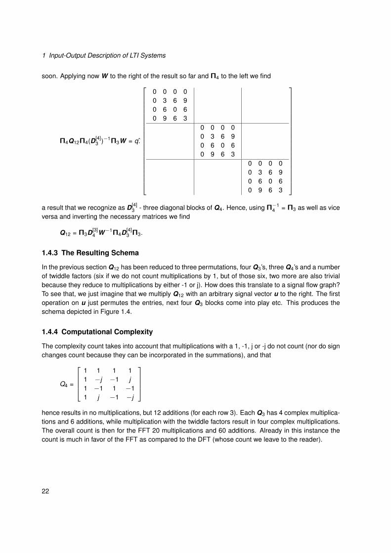
soon. Applying now W to the right of the result so far and Π4 to the left we find

Π4Q12Π4(D[4]3 )−1Π3W = q .

0 0 0 00 3 6 90 6 0 60 9 6 3

0 0 0 00 3 6 90 6 0 60 9 6 3

0 0 0 00 3 6 90 6 0 60 9 6 3

a result that we recognize as D[4]3 - three diagonal blocks of Q4. Hence, using Π−1

4 = Π3 as well as viceversa and inverting the necessary matrices we find

Q12 = Π3D[3]4 W−1Π4D[4]

3 Π3.

1.4.3 The Resulting Schema

In the previous section Q12 has been reduced to three permutations, four Q3’s, three Q4’s and a numberof twiddle factors (six if we do not count multiplications by 1, but of those six, two more are also trivialbecause they reduce to multiplications by either -1 or j). How does this translate to a signal flow graph?To see that, we just imagine that we multiply Q12 with an arbitrary signal vector u to the right. The firstoperation on u just permutes the entries, next four Q3 blocks come into play etc. This produces theschema depicted in Figure 1.4.

1.4.4 Computational Complexity

The complexity count takes into account that multiplications with a 1, -1, j or -j do not count (nor do signchanges count because they can be incorporated in the summations), and that

Q4 =

1 1 1 11 −j −1 j1 −1 1 −11 j −1 −j

hence results in no multiplications, but 12 additions (for each row 3). Each Q3 has 4 complex multiplica-tions and 6 additions, while multiplication with the twiddle factors result in four complex multiplications.The overall count is then for the FFT 20 multiplications and 60 additions. Already in this instance thecount is much in favor of the FFT as compared to the DFT (whose count we leave to the reader).

22


!Figure 1.4: Signal Flow Graph for Computing the FFT. Twiddle Factors colored are colored in annotated with theirrespective coefficient of q.

23


1.4.5 Generalization

The theory so far generalizes easily to the product N = r · s and two (dual) schemas will be obtained,one for r · s and one for s · r . Using the notation developed in this chapter and adapted to the newsituation we can write

Qr ·s = Πr D[r ]s W−1ΠsD[s]

r Πr ,

where some attention has to be devoted to the structure of the twiddle factor matrix. It will consist of rdiagonal blocks of dimension s

W = diag {W0, W1, ... , Wr−1}

with

Wj = diag {1, qj , ... , qs−1},

in particular W0 is a unit matrix and the maximum power of q is (r − 1)(s − 1).For a comprehensive presentation on various forms of the Fast Fourier Transformation I recommend

to consult with the excellent book by Charles van Loan [4].

1.5 Fast Convolution via FFT

The convolution operation costs O(N2) operations, if N is the length of the signals we are working on.Alternatively, exploiting the convolution theorem of the Discrete Fourier Transformation we can computethe output signal of a linear time-invariant system in the frequency domain. The Discrete Fourier Trans-formation of a given signal can be computed very efficient way by the Fast Fourier Transform (FFT). Thisleads to the so-called Fast Convolution method, which requires O(N log N) operations. This denotes asignificant saving in computations when comparing the Fast Convolution with the direct execution of theconvolution sum. Figure 1.5 shows the detour through frequency domain for computing the convolution.

This frequency domain method using the FFT works very well, is well established and it’s efficiencycan be regarded as one of the major cornerstones for the tremendous success of digital signal pro-cessing during the past 30 years. However, it is based on the assumption that the systems involved arelinear and time-invariant. If one of these two assumptions is violated, then the use of frequency domaintools is no longer applicable. If the system is time-varying, then the impulse response changes withtime. That implies that the columns in the convolution operator T are not shifter versions of the impulseresponse [tk ] and hence the operator looses its Toeplitz property. Also, the cyclic Toeplitz matrix doesnot exist anymore, which is the cornerstone for the matrix Q to consist of the eigenvectors of T c andhence the convolution theorem of the Discrete Fourier Transform does not hold anymore.

Successfully and efficiently computing in the Fourier domain is also fitting only if the impulse re-sponses [tk ] describing the input-output behavior of the system has finite length. In signal processingapplications engineers use recursive filters, which have a finite number of parameters but which producean impulse response of infinite length. We will deal this case in coming sections.

24

1.5 Fast Convolution via FFT

Convolution

Fast Convolution

Pointwise Multiplication

FFT IF

FT

[tk], [uk][tk] � [uk]

[yk]

F{[yk]}F{[uk]}, F{[tk]} F{[uk]} · F{[tk]}

Time Domain

Frequency Domain

Figure 1.5: Schematic Procedure for Computing Fast Convolutions.

25


1.6 Diagonal expansion of Toeplitz matrices

1.6.1 Infinite dimensional Toeplitz Matrix

For the further use of the Toeplitz matrices we introduce a slightly modified notation for dealing with theconvolution of sequences. This modified notation will open a new viewpoint onto the topic, a viewpointthat will carry us beyond some of the limitations arising from the use of Fourier techniques, notably thelimitation to handle time-invariant systems only.

For a system to be truly time-invariant, the impulse response is invariant for all times, i.e. the corre-sponding Toeplitz operator describing the system must be infinite dimensional, the convolution operationthen looks like

y = T · u =

...y−1

y0

y1

y2

y3

y4...

=

. . ....

......

.... . . t−1 t−2 t−3 t−4. . . t0 t−1 t−2 t−3

. . .. . . t1 t0 t−1 t−2

. . .. . . t2 t1 t0 t−1

. . .. . . t3 t2 t1 t0

. . .

t4 t3 t2 t1. . .

......

. . . . . . . . .

·

...u−1

u0

u1

u2...

. (1.19)

We are looking for a more compact notation to exploit the structure of the infinite dimensional Toeplitzmatrix. To this end we introduce the Shift Operator.

1.6.2 Shift Operator

The Toeplitz matrices in equation (1.19) have a very particular structure, that is, every column of thematrix is a down-shifted version of the previous column. We intend to exploit this shift-structure toestablish a notation and a formalism, which we can extend from linear tim-invariant to time-varyingsystems. To this end we introduce the Shift operator, which we denote by the symbol Z . The Shiftoperator has the function to shift all entries of a vector downward by one position. We can give thisdownward shift the interpretation of a temporal delay, that is,

uk = Zuk+1, k = −∞, ... ,∞.

For our matrix-oriented notation we will use the matrix representation Z for the shift operator, whichacts from the left on a given vector u and pushes all its entries down by one notch

Zu = Z

...u−1

u0

u1

u2...

7→

...u−2

u−1

u0

u1...

, Z−1u = Z−1

...u−1

u0

u1

u2...

7→

...u0

u1

u2

u3...

. (1.20)

26


The rectangular box indicates our reference of time origin. Likewise, the inverse also holds, that is,Z−1 acting on the vector u pushes the entries of the vector up by one notch. It is worth noting that withinfinite dimensional vectors and matrices, the shift operator Z is orthogonal, i.e. Z T Z = ZZ T = 1, sincefor infinite dimensional vectors, shifting up and down does not truncate the vectors. The matrix Z itselfis actually an infinite dimensional lower (causal) matrix

Z =

. . .

. . . 01 0

1 01 0

. . . . . .

, Z−1 = Z T =

. . . . . .0 1

0 10 1

0. . .. . .

.

Similarly, the shift operator and its inverse can also be applied to a row vector from the right uT Z[

... u−1 u0 u1 u2 ...]· Z =

[... u−1 u0 u1 u2 ...

],

shifting all vector entries one position to the left. Accordingly, we achieve a shift by one position to theright by post-multiplication of the row vector uT with the inverse shift operator, that is, we then have

[... u−1 u0 u1 u2 ...

]· Z T =

[... u−2 u−1 u0 u1 ...

].

We can also apply the shift operator simultaneously from the left and from the right to a matrix A suchas ZAZ T , which has the effect to push the entries of A down one slot along the diagonal, which lookslike

Z ·

A

· Z T =

. . .

A

.

We can push down the matrix along its diagonal by k slots if we apply the shift operators from the leftand from the right k times Z k A(Z T )k .

1.6.3 Superposition of Diagonals

Using the shift operator introduced in the previous section we can represent an infinite dimensionalToeplitz Operator (1.19) as the superposition of diagonals, such as

T = · · ·+

. . . . . .. . . t−1

. . . t−1. . . . . .

. . .

+

. . . . . .

. . . t0. . .

. . . t0. . .

. . . t0. . .

. . . . . .

+

. . .

. . . . . .

t1. . .

t1. . .. . . . . .

+...

27


This principle can be modified by denoting the values ti , i = −∞,∞ along the main diagonal andproviding the additional information by how many sub-diagonals this diagonal needs to be pushed downor pushed up. Pushing down by k diagonals is represented by the k -th power of the shift operator Z ,pushing up diagonals is accomplished be negative powers of Z . This amounts to writing the Toeplitzoperator as

T = · · · + Z−1 ·

. . .t−1

t−1. . .

+

. . .t0

t0. . .

+ Z ·

. . .t1

t1. . .

+ ...

· · ·+ Z−1diag {t−1} + Z 0diag {t0} + Z 1diag {t1} + Z 2diag {t2} + Z 3diag {t3} + · · · =∞∑

i=−∞Z i ·diag {ti }.

This notation reminds the reader of the z-transform of the time series {ti},−∞ < i <∞,

T (z) =∞∑

i=−∞tiz i ,

which can be thought of as an efficient manipulation tool when working with diagonals of infinite di-mensional Toeplitz-Operators. There exists an 1:1 relationship between the set of power series and theset of infinite dimensional Toeplitz-Operators. The validity of this mechanism relies on the fact that thevalues along a diagonal are all the same, which is a consequence of dealing with time-invariant sys-tems. Also note that in the context of the z-transformation the variable z is considered to be a complexvariable, whereas the shift operator is a real valued, infinite dimensional matrix.

1.6.4 Causality

We consider linear, time-invariant systems, which are given in terms of their Toeplitz matrix T . We feedthe systems with an input signal u, which starts with the value u0, that is at time index k = 0. We writethis up as

y = T · u =

...y−1

y0

y1

y2

y3

y4...

=

. . ....

......

.... . . t−1 t−2 t−3 t−4. . . t0 t−1 t−2 t−3

. . .. . . t1 t0 t−1 t−2

. . .. . . t2 t1 t0 t−1

. . .

t3 t2 t1 t0. . .

t4 t3 t2 t1. . .

......

. . . . . . . . .

·

...0u0

u1

u2...

.

28


We can see that the system produces a valid output signal

y−1 = t−1u0 + t−2u1 + t−3u2 ... ,

which appears at the output temporally before the input signal actually starts; the system behaves ina non-causal way. For a linear system to behave strictly causal, the corresponding Toeplitz operatorhas to be strictly lower triangular. The set of all causal systems corresponds with the set of all lowertriangular matrices and is denoted by the symbol L. The set of all upper triangular matrices, which wedenote by the symbol U , corresponds with the set of anti-causal systems. We use the symbol D todenote the set of diagonal matrices, i.e.

D = U ∩ L.

Note that there are situations where being able to handle non-causal systems is useful. Take for ex-ample image processing, where the pixels in a row are extending to the left and to the right without thenotion of time being important. However, we are not diving into this topic right now.

In Equation 1.21 we see a lower triangular Toeplitz matrix TL describing a causal system

y = TL · u =

...0y0

y1

y2

y3

y4...

=

. . ....

......

.... . . 0 0 0 0. . . t0 0 0 0

. . .. . . t1 t0 0 0

. . .. . . t2 t1 t0 0

. . .

t3 t2 t1 t0. . .

t4 t3 t2 t1. . .

......

. . . . . . . . .

·

...0u0

u1

u2

u3...

. (1.21)

Using the shift operator and the diagonal expansion discussed in the previous section we have a lookat the following example for a simple FIR filter

T (Z ) =12

Z−1 − 1 +12

Z ⇔ T =

. . . . . .

. . . −1 1/21/2 −1 1/2

1/2 −1 1/2

−1/2 −1. . .

. . . . . .

.

This tridiagonal system is non-causal, as it is able to produce output signals that lie temporally beforethe input signals. Take the causal part of this simple FIR filter, which is the lower triangular part of the

29


tridiagonal matrix

TL(Z ) =12

Z − 1 ⇔ T =

. . .

. . . −11/2 −1

1/2 −11/2 −1

. . . . . .

.

The strictly anti-causal part of the previously introduced FIR filter is described in terms of the uppertriangular part of the tridiagonal matrix T , i.e. by

TZ−1U (Z ) =12

Z−1 ⇔ T Z−1U =

. . .

. . . 0 1/20 1/2

0 1/20. . . . . .

,

where Z−1U denotes the strictly upper triangular part of a matrix and hence the strictly anti-causalsystems. We can identify the anti-causal parts of the system to be associated with negative exponentsof the shift operator.

30

2 State-Space Description of LinearTime-Invariant Systems

2.1 State-Space Model for Linear Systems

2.1.1 Reactance Extraction

A linear input-output system with input signal [uk ], impulse response [tk ] and the corresponding [yk ] istypically represented by the schematic drawing in Figure 2.1, where T denotes the Toeplitz matrix of

T {·}[uk] [yk]

Figure 2.1: A linear input-output system.

the linear convolution operator function for the impulse response [tk ]. In a next step the drawing of thesystem is slightly redrawn to produce the representation in the left part of Figure 2.2. The internals

T {·}[uk]

[yk]

T {·}

[uk]

[yk][xk]

[xk+1]

Σ Z

Figure 2.2: Alternative version for representing a linear system.

of the systems inside the dashed box will be further structured while the input-output relation T staysunchanged. The process of structuring we are about to embark has been called reactance extractionby Dante Youla [8]. Reactance extraction means that the internals of the block are separated into twocascaded sub-blocks as shown in the right part of Figure 2.2.

31

2 State-Space Description of Linear Time-Invariant Systems

The first block on left, labeled Σ contains non-dynamic components only, i.e. in an analog electronicsworld this amounts to resistors, ideal transformers and gyrators. In the realm of digital technology, theblock Σ contains only arithmetic operators (multiplication, division, addition, subtraction, square-roots,etc.) and connecting wires. Hence the function of the block Σ can be mathematically described byconstant matrices over the real or complex field.

The second block, labeled Z contains all dynamic components of the linear system. Again, in ananalog electronics world this amounts to inductances and capacitances, which are commonly referredto as ’reactances’ in classical network theory, hence the name ’reactance extraction’. Using digitaltechnology the dynamic components of the systems are delays, storages, registers, latches etc.

Such a cascaded structuring of the system introduces new variables at the interconnections betweenΣ and Z , which we denote by xk+1 and xk . This definition of variables also expresses the functionof the Z -block, which is to delay signals by one time-unit. If we were to deal with continuous timelinear systems, these variables would be replaced by x and x , respectively, and the function of theZ -block being an integration [9]. The description for our linear system which results from this approachis commonly referred to as the Kalman state-space description.

2.1.2 Resistance Extraction

For the sake of completeness we mention that there exists an alternative decomposition for the systemT . This alternative decomposition is called a Darlington model, where the Z -block now comprises allnon-dynamic elements of the system, which consume or produce energy, i.e. (positive and negative)resistors in an analog electronics world or simple real numbers in a digital domain. In correspondenceto the previous paragraph we can name this approach a ’resistance extraction’. The matrices, whichare used to describe such a Z -block are constant matrices. If all elements, which consume or produceenergy are comprised in the Z -block then the block Σ is left as a lossless transformation, which alsocontains all dynamic, or frequency-dependent parts. This can be translated into the Σ-block consistingof ideal transformers, gyrators, inductances and capacitances for an analog electronics box. The corre-sponding mathematical description is based on matrices over the field of rational functions, where thenotion of losslessness is expressed by the property that the corresponding matrices are para-unitary.We won’t go any further in this direction here and leave it as such.

Both possible decompositions of the system amount to very specific representations or parameteri-zations for rational functions. In the following we will make use of the state-space description accordingto a reactance extraction approach.

2.1.3 What’s a state anyway?

What characterizes the notion of state? Over the years the following insight has crystallized (see [5]).

The state at a given time t (or index k when discrete time) is sufficient information onthe system at that given time point t to predict its future evolution, given future inputsexclusively.

This means, among other things, that the whole past evolution of the system up to time t is, as far asthe future is concerned, fully accounted for in the state vector at time t , no more information on the pastis needed to assess the future evolution, given future inputs, or, to put it more negatively, the system

32

2.1 State-Space Model for Linear Systems

forgets everything from its past except what is contained in its state. This is somewhat illustrated in fig.2.3.

state x

&me t

past inputs that produce a given state the output produced by a state and a given (future) input

Past Future

Figure 2.3: The state as the link between past and future

2.1.4 State minimality

In the state description just given, the state is described as sufficient information. Minimality wouldactually require also necessary information. A computer memory is usually filled with all sorts of in-formation that is not relevant to the problem at hand. A state is called minimal when no data in thestate vector at time t can be left out without potentially affecting future outputs (more precisely: so thatno future input exists for which the system’s evolution would be different). This leads to the notion ofNerode equivalence: we say that two past inputs up to time t are Nerode equivalent, if there is no inputstarting at time t that will produce different future outputs. It should be immediately obvious that thenotion of minimality depends very much on the output equation as well: it may very well be that part ofthe system internals are not visible from the output. A completely autonomous system has no inputsnor outputs, so a minimal description for it would be empty. This unpleasant situation can be remediedby the convention that in the case of an autonomous system, one can observe the state directly, sothat the output equation simply becomes [yk ] = [xk ]. Since there are no inputs any more in this case,the state determines the output evolution uniquely. The great breakthrough of Newtonian mechanicswas the realization that the velocity of the planets belonged to the state, in contrast to what the ancientWestern world thought, limiting the state just to position data and making change of position directlydepend on force.

An important further consequence of the notion of minimal state is that the state quantities are al-gebraically independent. They can be assigned arbitrary values (of course within the number systemused, in our case they will be either real or complex numbers), independently from each other. Herealso, there is a potential unwarranted generalization. It is conceivable that independent state variablesmay only take limited sets of values. That is e.g. the case in a computer, which does not allow anysize of number, but also real life systems are limited by ranges of relevant variables. The mathematicalformalism conveniently ignores these contingencies, hoping that the theory shall be able to handle themwhen actually necessary.

33


2.2 State-Space Modelling

2.2.1 State-Space Equations

The Σ-block in the right part of Figure 2.2, which contains the non-dynamic components is furtherelaborated such that we arrive at a internal description as given in Figure 2.4. From the signal flowdiagram in Figure 2.4 we can read off a set of equations, which describe the internal workings of thesystem. The equations are

xk+1 = A · xk + B · uk

yk = C · xk + D · uk , (2.1)

using the matrices A ∈ Rn×n, B ∈ Rn×m, C ∈ Rp×n, D ∈ Rp×m. Here, at a time instant k , the

+

+

A

B

C

D

Σ =

�A BC D

�

Σuk

yk

xk+1

xk

Z

Figure 2.4: State-Space Model based on Reactance Extraction.

system is assumed to have m inputs (uk ∈ Rm) and p outputs (yk ∈ Rp), while n is the dimensionof the state-vector (xk , xk+1 ∈ Rn), which again corresponds with the dynamic degree for this system(determined by the dynamic sub-block). We conveniently combine the state-equations (2.1) into a morecompact matrix notation

[xk+1

yk

]=[

A BC D

]·[

xk

uk

], Σ =

[A BC D

], (2.2)

34


which expresses the signals coming out of the Σ-block in terms of signals going in the block. We canassociate the interpretation of the matrix Σ given in Equation 2.2 as being the scattering matrix of themulti-port Σ.

2.2.2 Impulse Response

The input-output behavior of a linear, time-invariant system is characterized by its impulse response.We identify the impulse response [tk ] pertaining to the system model shown in Figure (2.4) by graphicalinspection. We assume the system to start out with no data stored in memory. We use a single impulseu0 = 1 at time index k = 0 after which we will not have any more input signals. We follow this impulsesignal as it propagates through the signal flow graph in Figure (2.4) allowing us to read off the values ofthe impulse response [tk ] as the appear at the output [yk ]. The following table summarizes the findings.

k 0 1 2 3 4 ...

[uk ] 1 0 0 0 0 ...[xk ] 0 B AB A2B A3B ...[tk ] D CB CAB CA2B CA3B ...

.

The values of the impulse response for a system with zero initial conditions are given by

tk =

0 for k < 0,D for k = 0,CAk−1B for k = 1, 2, ...

(2.3)

2.2.3 Transfer Function

Block-Diagonal Representation

The transfer function describes the mapping of the input sequence [uk ] onto the output sequence [yk ](complete sequences). In this section we derive a representation of the transfer function T , which isparametrized in terms of the quantities of the state-space model, i.e. in terms of the matrices A, B, C, D.

We want to use only purely purely algebraic concepts to arrive at a compact representation ofthe Toeplitz operator T , such that we can replace the complex-valued transfer function T (z) (z-transformation), which is restricted to the time-invariant case. We first acknowledge that we need ablock diagonal expansion of the state-space equations all diagonal blocks are identical, that is, we have

A =

. . .A

AA

. . .

B =

. . .B

BB

. . .

35


C =

. . .C

CC

. . .

D =

. . .D

DD

. . .

,

which also leads to a block diagonal form for the realization matrix

Σ =[

A BC D

].

The shift operator basically stays the same (except that all identity matrices have identical dimension)

Z =

. . .

. . . 01 0

1 0

1. . .. . .

.

Using these conventions we build infinite-dimensional vectors x ,u and y , which contain a sequence ofstate-vectors, input values and output values, respectively, i.e. we use

x =

...xk−2

xk−1

xk

xk+1...

, u =

...uk−2

uk−1

uk

uk+1...

, y =

...yk−2

yk−1

yk

yk+1...

,

where the square around the vector xk indicates the position of the state-vector pertaining to the currenttime index. We employ the shift operator Z , which denotes the pushing down of the elements in a vectorby one notch, i.e. we use it to push the vector x up such as

...xk−1

xk

xk+1

xk+2...

= Z−1 ·

...xk−2

xk−1

xk

xk+1...

= x ↑ .

36


State-Space and Transfer Function in Block Diagonal Notation

Using our new notational conventions and reviewing Equations (2.1) we can re-formulation of the state-space equation for entire sequences

Z−1x = Ax + Bu

y = Cx + Du. (2.4)

Our goal is to determine an algebraic representation for the transfer function. To this end we need toeliminate the state-variable x from Equation 2.4 to arrive at the desired formula for T u = y . From thefirst equation we can determine

(In − ZA)x = ZBu → x = (In − ZA)−1ZBu

Inserting this equation into the second part of Equation (2.4) we arrive at

y =[D + C(In − ZA)−1ZB

]· u,

from which we can directly read off the transfer function T , which is a compact representation of theToeplitz operator T in terms of the linear fractional map

T = D + C(In − ZA)−1ZB. (2.5)

Notice that this algebraic representation of the transfer function of a linear time-invariant system asgiven in Equation 2.5 looks structurally identical to the conventional formulas for the transfer function interms of state-space quantities, which the reader may recall from text books on the topic. However, in atraditional context the variable z represents a complex number while in the current context the variableZ represents the shift-operator, which we can represent as a (infinite dimensional) matrix, which isaltogether a different kind of object.

Neumann Expansion

In order to verify the validity of the representation in Equation (2.5), we first want to deliberate on theresolvent

(1 − ZA)−1 = 1 + ZA + (ZA)2 + (ZA)2 + ... (2.6)

= 1 + ZA + ZAZA + ZAZAZA + ... (2.7)

= 1 + ZA + Z 2A2 + Z 3A3 + ... , (2.8)

where we use the Neumann expansion (1− X )−1 = 1 + X + X 2 + X 3 + ... , ‖X‖ < 1, which structurallyresembles the geometric series. The series in Equation 2.8 converges if the matrix A has all its eigen-values inside the unit disk. If this condition is satisfied, then the term (1 − ZA) is boundedly invertible.This property corresponds to well-known stability statements for state-space systems.

For this derivation based on the Neumann expansion to hold, we need to verify that the shift-operatorZ commutes with the block-diagonal matrix A, i.e. we need to check if

ZA = AZ

37


hold. For time-invariant systems (infinite dimensional matrices) with constant block-diagonals shiftingdown of the block-diagonal matrix (pre-multiplication with Z ) has the same effect then shifting left (post-multiplication with Z ). We observe

ZA =

. . .

. . . ↓A ↓

A ↓A

. . .

. . .

=

. . .

. . . ←A ←

A ←A

. . .

. . .

= AZ .

Putting together the series expansion in Equation (2.8) we generate a matrix representation

(1 − ZA)−1 =

. . .

. . . 1

. . . A 1

. . . A2 A 1

. . . A3 A2 A 1...

.... . . . . . . . .

.

Here we can easily see that it takes a matrix A to have all its eigenvalues inside the unit disk for thisexpression to converge to a bounded matrix.

Putting it all together

With the result from the previous subsection (Neumann expansion) we can evaluate the formula for thetransfer function

C (1 − ZA)−1 ZB =

in a step-by-step fashion

=

. . .C

CC

. . .

·

. . .

. . . 1

. . . A 1

. . . A2 A 1

. . . A3 A2 A 1...

.... . . . . . . . .

·

. . .

. . . 0B 0

B 0. . . . . .

38


to finally arrive at the matrix

C (1 − ZA)−1 ZB =

. . .

. . . 0

. . . CB 0

. . . CAB CB 0

. . . CA2B CAB CB 0...

. . . . . . . . . . . .

.

Adding to his intermediate result the diagonal block matrix containing the Ds

T =

. . .

. . . 0

. . . CB 0

. . . CAB CB 0

. . . CA2B CAB CB 0...

. . . . . . . . . . . .

+

. . .D

DD

. . .

completes the derivation. We finally have established the transfer function representation for a linear,time-invariant and causal system

T =

. . .

. . . D

. . . CB D

. . . CAB CB D

. . . CA2B CAB CB D...

. . . . . . . . . . . .

.

Looking at the matrix T we can identify it to be a Toeplitz matrix. Comparing its entries with Equation 2.3reveals that T consists of columns, which are shifted versions of the impulse response. This coincideswith the statements made in the previous section dealing with the linear convolution operation. Thisresult also underlines the equivalence of the transfer function and impulse response for characterizinga linear, time-invariant system.

This subsection establishes that a purely algebraic representation of the Toeplitz operator in terms ofthe linear fractional map works well for time-invariant systems. The structure of the matrices involvedclearly indicates a road map to generalize this approach to also describe time-varying systems. Inmore detail, we will see that we take into account a slightly more complicated notation as well as aclose inspection of the Neumann expansion to see if this can be generalized to the time-varying case.

39


2.3 State-Space Equivalence

2.3.1 State Transformation

For a given transfer function there exists an infinite number of realizations. Each realization corre-sponds with a particular set of state-space equations. All these realizations and hence their corre-sponding state-space equations are connected providing a parametrized representation capturing thecorresponding degrees of freedom. To this end we investigate the effect of a change of coordinatesin the state-space, which we perform by means of a non-singular transformation of the state-spacecoordinates.

It is permissible to transform the coordinates of the state-space with a non-singular transformation R,

x ′k+1 = R · xk+1, or R−1 · x ′k = xk .

The corresponding blocks are inserted in the system model and shown in Figure 2.5. Substituting the

+

+

A

B

C

D

uk

yk

xk+1

xk

ZR

R−1

x�k+1

x�k

Σ� =

�RAR−1 RBCR−1 D

�

Figure 2.5: Transformation of State-Space

transformed state-variables in the state-equations with the goal to represent the linear system in termsof the new variables x ′ results in the expressions

R−1 · x ′k+1 = A · R−1x ′k + Buk

yk = C · R−1x ′k + Duk ,

which will then directly lead to the transformed state-space representation[

x ′k+1yk

]=[

R1

]·[

A BC D

]·[

R−1

1

]·[

x ′kuk

], (2.9)

40

2.3 State-Space Equivalence

with the transformed realization matrix

Σ′ =[

A′ B′

C′ D′

]=[

RAR−1 RBCR−1 D

].

We can see that the state-space transformation induces a similarity transformation RAR−1 on the matrixA. Similarity transformations leave the eigenvalues of a matrix invariant, i.e. the matrices A and RAR−1

have the same eigenvalues.Using our block diagonal notation we can formulate this transformation directly as

x ′ = R · x ⇒

...

x ′kx ′k+1

...

=

. . .

RR

. . .

...xk

xk+1...

.

Similar to the steps before (Equ. 2.9) we plug in this state-transformation into the state-space equationsin block diagonal notation to produce

...

x ′k+1

x ′k+2...

=

. . .

RAR−1

RAR−1

. . .

...

x ′kx ′k+1

...

+

. . .

RBRB

. . .

...uk

uk+1...

,

for the state-equation and as

...yk

y ′k+1...

=

. . .

CR−1

CR−1

. . .

...

x ′kx ′k+1

...

+

. . .

DD

. . .

...uk

uk+1...

for the output equation. We can represent both equations more compactly by the fat notation

Z−1x ′ = RAR−1x ′ + RBu

y = CR−1x ′ + Du, (2.10)

which reveals that the block diagonal notation produces structurally the same result as Equation 2.9in a purely algebraic way. The block diagonal version of the transformed state-space realization thenbecomes

Σ′ =[

A′ B′

C′ D′

]=[

RAR−1 RBCR−1 D

].

Even though the block diagonal notation appears unnecessarily clumsy it offers the opportunity to alsodescribe time-varying systems in a seamless way preserving the structure of the fundamental approach.

41


2.3.2 Invariance of Transfer Function and Impulse Response

The transfer function T is invariant under non-singular transformations of the state-space with R, i.e.the matrices Σ and Σ′ are realizations for the same transfer function T . This can be shown by thefollowing computation

T ′ = D′ + C′(1 − ZA′)−1ZB′

= D + CR−1(1 − ZRAR−1)−1ZRB

= D + C(1 − ZA)−1ZB

= T .

The invariance of the transfer function can also be shown by showing the invariance of the correspond-ing impulse response. The impulse response t ′k can be read off from the block diagram in Figure (2.5),which includes the state transformation R. The impulse response t ′k is compared to the impulse re-sponse tk identified by inspection of the system shown in Figure (2.4)

k 0 1 2 3 4 ...

t ′k D CR−1RB CR−1RAR−1RB CR−1(RAR−1)2RB CR−1(RAR−1)3RB ...

tk D CB CAB CA2B CA3B ...

.

It is clearly visible, that the effect of the transform R cancels out leaving the impulse response andhence the transfer function invariant. The effect of the transformation R is similar to an all-pass filter,which can not be identified by looking at the input-output map. The transfer function of the systemstays identical, yet the realization can change. Hence, there is no unique realization for a given transferfunction. The set of all possible realizations for a given transfer function is parameterized in terms of thenon-singular matrix R. Since there exist infinitely many non-singular matrices R there also exist infinitelymany realizations for a particular transfer function. This has a very important consequence - starting outwith any realization Σ for a given T the transformation R can be employed in an optimization scheme tofind an alternative realization Σ′, which minimizes e.g. the arithmetic cost, or which minimizes round-offnoise, or coefficient sensitivity or any other conceivable cost function.

2.4 State-Space Arithmetic

We have two Toeplitz matrices T 1 and T 2. For each matrix we have a corresponding state-spacerealizations

T 1 ↔ Σ1 =[

A1 B1

C1 D1

], T 2 ↔ Σ2 =

[A2 B2

C2 D2

].

to allow for the representations

T 1 = D1 + C1 (1− ZA1)−1 ZB1 and T 2 = D2 + C2 (1− ZA2)−1 ZB2.

In order to develop matrix algorithms that directly work in state-space we need to determine elementaryarithmetic operations on matrices in state-space in terms of the state-space realizations for T 1 and T 2

42


u

u1 u2 y2y1

y

T1 T2

TS

�A2 B2

C2 D2

��A1 B1

C1 D1

�

y1

�A1 B1

C1 D1

�

y2

�A2 B2

C2 D2

�

Figure 2.6: State-Space Realization for sum of two matrices

2.4.1 Addition

Determine an expression for a possibly non-minimal state-space realization ΣA for the addition of twomatrices, i.e.

T A = T 2 + T 1

in terms of the state-space realizations for T 1 and T 2 (see Figure 2.6).For the sum of the two systems we can add the output equations

yk = y [1]k + y [2]

k = C[1]x [1]k + C[2]x [2]

k + D[1]uk + D[2]uk .

For the state equations we have

x [1]k+1 = A[1]x [1]

k + B[1]uk , x [2]k+1 = A[2]x [2]

k + B[2]uk .

Combining the equations into one block matrix notation and using the state-vector xk =

[x [1]

kx [2]

k

]we get

the realization matrix

ΣS =

[

A[1] 00 A[2]

] [B[1]

B[2]

]

[C[1] C[2]

][D[1] + D[2]]

(2.11)

Note that even if the realizations for the two matrices T 1 and T 2 are minimal realizations, the realizationaccording to equation (2.11) does not have to be minimal.

43


T1 T2

�A2 B2

C2 D2

��A1 B1

C1 D1

�

�A1 B1

C1 D1

� �A2 B2

C2 D2

�

Tp

[uk]1 [uk]2 [yk]2[yk]1

[yk][yk]1

[uk]1

Figure 2.7: State-Space Realization for product of two matrices

2.4.2 Multiplication

Determine an expression for a possibly non-minimal state-space realization ΣP for the product ofmatrices

T P = T 2 · T 1

in terms of the state-space realizations for T 1 and T 2 (see Figure 2.7).For the product of two matrices we can use the relations u[1]

k = uk , u[2]k = y [1]

k and yk = y [2]k to formulate

the output equations according to

y [1]k = C[1]x [1]

k + D[1]uk ,

which we can plug in to get

yk = C[2]x [2]k + D[2]y [1]

k = C[2]x [2]k + D[2](C[1]x [1]

k + D[1]uk ) =[

D[2]C[1] C[2]][

x [1]k

x [2]k

]+ D[2]D[1]uk .

Expanding the state equations and combining them into a block matrix using the extended state vector

xk =

[x [1]

kx [2]

k

]we arrive at

[x [1]

k+1x [2]

k+1

]=[

A[1] 0B[1]C[1] A[2]

][x [1]

x [2]

]+[

B[1]

B[2]D[1]

]uk .

Putting all equations together we can directly identify the realization matrix

ΣP =

A[1] 0 B[1]

B[2]C[1] A[2] B[2]D[1]

D[2]C[1] C[2] D[2]D[1]

(2.12)

Note that even if the realizations for the two matrices T 1 and T 2 are minimal realizations, the realizationaccording to equation (2.12) does not have to be minimal.

44


T1 T2

�A2 B2

C2 D2

��A1 B1

C1 D1

�

�A1 B1

C1 D1

�

�A2 B2

C2 D2

�

TF

[yk]

[yk]1 [yk]2[uk]2[uk]1

[ek][uk]

Figure 2.8:

2.4.3 Feedback

Determine an expression for a possibly non-minimal state-space realization ΣF for the system depictedin Figure 2.8

The feedback connection of the two systems induces the identities u[1]k = uk + y [2]

k , yk = y [1]k and

u[2]k = yk producing a Toeplitz operator of the form

T F = (1− T 1T 2)−1T 1.

The realization for this Toeplitz operator can be determined by straight forward but tedious calculations

ΣF =

A[1] B[1]C[2] B[1]

0 A[2] 00 0 0

+

B[1]D[2]

B[2]

1

(1− D[1]D[2])−1 [ C[1] D[1]C[2] D[1]

].

2.4.4 Inversion

In many applications we are interested to determine the inverse of the transfer function T . Hence, weseek a state-space representation for the transfer function T−1.

We derive the state-space realization for the inverse system given the state-space realization for Tby looking at equation (2.2)

[xk+1

yk

]=[

A BC D

]·[

xk

uk

],

45


[uk]

[yk]

[xk]

[xk+1]

ZΓT−1

Γ =

�A−BD−1C BD−1

−D−1C D−1

�

Figure 2.9: Inverse realization of linear system.

46

2.5 Inversion of a lower triangular Toeplitz matrix

and by rearranging this equations in order to express the input uk and the state-variable xk+1 in termsof the output yk and the state-variable xk . Some elementary algebraic manipulations produce the result

[xk+1

uk

]=[

A− BD−1C BD−1

−D−1C D−1

][xk

yk

],

where the matrix

Γ =[

A− BD−1C BD−1

−D−1C D−1

], (2.13)

represents a state-space realization for the system that has the transfer function which is the inverse ofT . This realization exists if D is non-singular. Notice that Γ is not the inverse of Σ, but rather denotes astate-space realization for T−1.

This leads us to an interesting approach for computing matrix inversions. All we need is a state-spacerealization in terms of the A, B, C, D matrices. With such a realization we can directly exploit Equation(2.13) to determine a state-space realization for T−1. Via the mechanism given in Equation (4.2) wecan determine the inverse matrix T−1. Under certain conditions, this de-tour actually turns out to be ashort-cut for computing matrix inversions efficiently.


2.5.1 Bounded Inverse

Consider the infinite Toeplitz matrix of a time-invariant system given by the lower bi-diagonal matrix

T =

. . .

. . . 1−1

2 1−1

2 1−1

2 1−1

2 1. . . . . .

.

Since T is an infinite dimensional Toeplitz matrix we can use the conventional z-transform (conventionalexcept for the sign in the exponent !) to represent this Toeplitz matrix as

T = 1− 12

Z .

We want to calculate the inverse of this matrix. To this end we can use the z-transform tools to directlyhandle with infinite dimensional Toeplitz matrices, i,e. we can invert the matrix directly via

T−1 = (1− 12

Z )−1 =1

1− 12Z

= 1 +12· Z +

14· Z 2 +

18· Z 3 +

116· Z 4 − ... .

47


The series expansion for the inverse matrix converges as there are no poles inside of the unit disk(|z| < 1). Using this series expansion we can build up the infinite dimensional Toeplitz matrix of theinverse, given by

T−1 =

. . .

. . . 1

. . . 12 1

. . . 14

12 1

. . . 18

14

12 1

. . . 116

18

14

12 1

. . . . . . . . . . . . . . . . . .

.

2.5.2 Unbounded Inverse

Consider the infinite Toeplitz matrix of a time-invariant system given by the lower bi-diagonal matrix

T =

. . .

. . . 1−2 1

−2 1−2 1

−2 1. . . . . .

.

This matrix, we can also represent using conventional z-transformation notation, i.e. we can write

T = 1− 2Z .

Calculating the inverse of this matrix amounts to

T−1 = (1− 2Z )−1 =1

1− 2Z= 1 + 2 · Z + 4 · Z 2 + 8 · Z 3 + 16 · Z 4 − ... .

Converting this representation back into matrix notation we get

T−1 =

. . .

. . . 1

. . . 2 1

. . . 4 2 1

. . . 8 4 2 1

. . . 16 8 4 2 1. . . . . . . . . . . . . . . . . .

.

48


It is apparent that the the inverse matrix is not bounded, as its entries are growing boundlessly. This isunderstandable as we can see that the transfer function description of the inverse matrix obviously hasa pole inside the unit disk, which means that is an unstable system and that the series is not converging.In other words, this particular matrix T does not have a lower triangular and bounded inverse. yet inother words, this causal system does not have a causal inverse.

Using standard techniques from z-transformation we can do the following algebraic manipulations

T−1 = (1− 2Z )−1 =−1

2Z−1

1− 12Z−1

= −12

Z−1 − 14

Z−2 − 18

Z−3 − 116

Z−4 − ... ,

which yields an expression for the inverse matrix, which turns out to be a strictly upper triangular matrixcorresponding to an anti-causal, but bounded system, i.e. we get

⇒ T−1 =

. . . . . . . . . . . . . . . . . .0 −1

2 −14 −1

8 − 116

0 −12 −1

4 −18

. . .

0 −12 −1

4. . .

0 −12

. . .

0. . .. . .

.

Once you are confined to the domain of finite dimensional matrices it appears as an odd result to havean inverse of a lower triangular matrix that is upper triangular. However, our intuition may be restored ifwe observe what happens if we take a finite dimensional cut from the infinite matrix and if we displacethe main diagonal by one position towards the north-east.

T =

−2 1−2 1

−2 1−2 1

−2

.

For an infinite dimensional matrix, this displacement of the main diagonal must be negligible, i.e. theshifted matrix is almost lower triangular. The inverse of the shifted matrix can then be determined as

T−1 =

−12 −1

4 −18 − 1

16 − 132

−12 −1

4 −18 − 1

16−1

2 −14 −1

8−1

2 −14−1

2

.

49


Z Z Z

b1 b2 b3 y

u x1 x2 x3

b0

Figure 2.10: Finite Impulse Response filter; direct realization for n = 3

2.6 Direct Form State-Space Realizations

2.6.1 Moving Average (MA) Filter

We now consider a rather simple transfer function, given as the polynomial

T (z) = B(z) = b0 + b1z + b2z2 + · · · + bnzn.

We call the realization for this transfer function commonly as a Transversal Filter, or by the abbreviationFIR-Filter, which stands for Finite Impulse Response filter, or as a Moving Average (MA) filter. Sincethis transfer function is characterized by the zeros of the polynomial it is also termed a All-Zeros filter.The signal flow graph of the transversal filter is depicted in Figure ??.

The corresponding state-space realization is given in terms of

[A BC D

]=

0 11 0 0

. . . . . ....

1 0 0b1 b2 ... bn b0

2.6.2 Autoregressive (AR) Filter

Another simple transfer function is given as

T (z) =1

A(z)=

1a0 + a1z + a2z2 + · · · + anzn

which we denote either as an Autoregressive (AR) filter, or as a recursive filter. We also find the namesIIR-filter, where the abbreviation stands for Infinite Impulse Response filter. Since this transfer functionis characterized by the zeros of the polynomial A(z), which are the poles of the transfer function theterm All-Pole filter is also used. The signal flow of a direct realization for this transfer function is shownin Figure (2.11). The corresponding state-space realization matrix ist given as

50


Z Z Z a1 a2 a3

y u x1 x2 x3

Figure 2.11: All Pole Filter direct realization for n = 3

51


x3 x2 x1[yk]

[uk]b3 b2 b1

�a1 �a2 �a3

Z Z Z

Figure 2.12: Observability Canonical Form for the rational transfer function T (z)

[A BC D

]=

a1 a2 ... an 11 0 0

. . . . . . 0

1 0...

1 0 ... 0 0

.

2.6.3 Rational Transfer Fucntion

We consider a rational transfer function, which describes the input-output mapping of an ARMA-Filter(Autoregressive-Moving Average Filter). As the name suggests, this filter is combination of the twosimple forms we encountered in the previous section. The transfer function of rational degree n is givenas

T (z) =B(z)A(z)

=b0 + b1z + b2z2 + · · · + bnzn

a0 + a1z + a2z2 + · · · + anzn .

We want to have a minimal state-space realization for this transfer function. One such realization isgiven by the state-space realization matrix in equation (2.14), i.e. we have

[A BC D

]=

0 1 b1

0. . . b2. . . 1

...−an −an−1 ... −a1 bn

1 0 ... 0 0

. (2.14)

The corresponding signal flow diagram for this realization is depicted in Figure 2.12. This particularform of a realization is called a direct realization, because it directly uses the coefficients of the rationaltransfer function. In particular, this direct form is termed the observability canonical form. The use ofthe adjective canonical expresses the property of this realization to use the minimal number of delayelements, which coincides with the dynamical of the transfer function.

52


Z Z Z b3 b2 b1

-‐a1 -‐a2 -‐a3

y

u x3 x2 x1

Figure 2.13:

2.6.4 Canonical Form

There exists an infinite number of realizations for a given transfer function. Currently, we are interestedto see an alternative realization for the rational transfer function

T (z) =B(z)A(z)

=b0 + b1z + b2z2 + · · · + bnzn

a0 + a1z + a2z2 + · · · + anzn .

Figure 2.13 shows such an alternative realization.The corresponding state-space realization matrix ist given as

[A BC D

]=

0 1 0. . . . . . 0

0 1...

−an −an−1 ... −a1 1b1 b2 ... bn 0

.

53

3 Properties of State-Space Realizations

3.1 Controllability and Observability

3.1.1 Controllability

The evolution of a system’s internal state [xk ] is driven by the input sequence [uk ]. States that can begenerated by at least one past input are called reachable. If we can devise a sequence of input valuesthat steers the sequence of states to reach the zero-state starting from any reachable state, then thesystem is called controllable. However, it may be that some states at some time point k cannot bereached, i.e., there is no past input up to time k that is able to produce that particular state. We ask foran algebraic criterion to check for the controllability of a given system.

The controllability matrix C describes how input data from the past will be mapped into the internalstate of the system. The name originates from controlling the values for the internal state by a choice ofthe input signal. In order to devise formal criteria for investigating the property of controllability we usethe controllability matrix, which as defined as

C =[

B AB A2B A3B · · · An−1B ...]

, (3.1)

where A ∈ Rn×n and B ∈ Rn×q . The concept of the Controllability matrix is schematically depictedin Figure (3.1). The controllable subspace Xc of Σ is spanned by the columns of C and contains allcontrollable states.

Z

OC

Internal States

[uk] [yk]

Σ

Figure 3.1: Controllability and Observability.

55


The Cayley-Hamilton theorem states that rank of the controllability matrix and the span of its columnsare determined by the first n columns in C. For computational purposes the following (finite) controlla-bility matrix is of importance

Cn =[

B AB A2B A3B · · · An−1B]

.

The system Σ is (completely) controllable if the dimension of the controllability space Xc is n. This canbe expressed as dimXc = n or by rank (Cn) = n.

3.1.2 Controllability Gramian

A Gramian matrix is a tool to analyze the geometric properties of vectors, which span a vector space.In particular, the Gramian indicates the angles between these vectors, their Euclidean length as well asthe dimension of the spanned space. The columns of the controllability matrix C span the controllabilityspace. For this space, the Controllability Gramian is defined as

W := C · CT (3.2)

=[

B AB A2B · · ·]·

BT

BT AT

BT A2T

...

= BBT + ABBT AT + A2BBT A2T+ · · · =

∑

i

Ai (BBT )Ai T (3.3)

= BBT + A[BBT + ABBT AT + ...

]AT (3.4)

W = BBT + AWAT . (3.5)

The system Σ is (completely) controllable if the controllability Gramian W is a symmetric positivedefinite matrix.

The last equation is commonly referred to as a Lyapunov equation. This implies that the Controlla-bility GramianW appears as a symmetric positive definite solution of the Lyapunov equation.

3.1.3 Observability

The behavior of a linear system is largely determined by the evolution of state vectors [xk ]. However,in many technical situations we do not have the possibility to observe the value of the state vectorexplicitly, but only as some sort of linear combination of state vectors visible at the output sequence[yk ]. The observation problem is then to formulate conditions under which the observer of the outputsignal can reconstruct the sequence of state vectors.

It happens that some states will produce the same output in the future, no matter which future inputis applied. The distinction between such states is called unobservable, one may change any suchstate into another one in the collection without being able to observe the change. We call the stateobservable, when each such equivalence class of states that all produce the same future output forwhatever future input consists of only one element. Actually, every equivalence class of states whosedistinction is unobservable can be represented by just one state.

56

3.1 Controllability and Observability

The observability matrix O describes how the internal states will be mapped into the future outputsignal. This way, the internal state represents all the system needs to memorize from signals in the pastto determine the output in the future. If this process does not imply information loss, then the observercan retrieve the state information. To characterize this feature we use the observability matrix of Σ,which is defined as

O =

CCACA2

CA3

...CAn−1

...

, (3.6)

where A ∈ Rn×n and C ∈ Rp×n. The concept of the Observability is schematically depicted in Figure(3.1). Again, the Cayley-Hamilton theorem says that the observability space Xo is determined by thefirst n rows of O. For computational reasons we consider the finite observability matrix

On =

CCACA2

CA3

...CAn−1

The system Σ is (completely) observable if the dimension of the observability space Xo is n, which wecan express either as dimXo = n or, equivalently by stating that rank (On) = n.

3.1.4 Observability Gramian

The rows of the observability matrix O span a subspace, the observability space. For this space, theGramian is defined as

K := OT · O (3.7)

=[

CT AT CT A2T CT ...]·

CCACA2

...

(3.8)

= CT C + AT CT CA + A2TCT CA2 + · · · =

∑

i

Ai T (CT C)Ai (3.9)

= CT C + AT [CT C + AT CT CA + ...]

A (3.10)

K = CT C + ATKA. (3.11)

57


The system Σ is (completely) observable if the Observability GramianK is a symmetric positive definitematrix. The last equation is commonly referred to as a Lyapunov equation. That is, the ObservabilityGramian K appears as a symmetric positive definite solution of the Lyapunov equation.

3.1.5 Gramian Matrices and State Transformations

We have seen that the concept of state transformation delivers an important to parametrize all realiza-tions for a given transfer function. We derived the equations to describe the corresponding transforma-tion mechanisms for the realizations. Similarly, we investigate the effect of a state-space transformationwith a non-singular matrix R on the Gramians. The effect on the observability and controllability matrixcan be seen to be

O′ = OR−1, C′ = RC.

The product of Controllability and Observability matrices remains invariant under state transformations

O′C′ = OR−1RC = OC,

while the Gramians undergo congruence transforms with the matrix R and R−1 according to

K′ = O′TO′ = R−1TKR−1, W ′ = C′C′T = RWRT .

A congruence transformation changes the eigenvalues, while leaving their sign invariant. The state-space transformation produces a similarity transformation of the product of the Gramians

K′W ′ = R−1TKWRT ,

which leads to the conclusion that K′W ′ and KW share the same eigenvalues.

3.1.6 Minimality and Stability

A system Σ that is completely observable and completely controllable is a minimal system. That meansthat the realization Σ comprises the minimum number of storage elements for realizing a given transferfunction T . A non-singular state transformation R does not change the observability or controllabilityproperties of a system realization.

3.2 Normal Forms for State-Space Realizations

With the help of the Gramian matrices we can specify three normal forms for state-space realizations.Starting out with any realization matrix Σ we use state-space transformations to transform it into one ofthe normal forms. This procedure makes use of the realization matrix

Σ =[

RAR−1 RBCR−1 D

], (3.12)

which includes the state transformation matrix R.

58

3.2 Normal Forms for State-Space Realizations

3.2.1 Input Normal Realization

A state-space realization Σ, which satisfies

CCT =W = 1

is called an input normal realization. With the goal to determine an input normal realization we can startout with controllability Gramian including a non-singular matrix R as a parameter, which we can denoteas

W ′ = RBBT RT + RABBT AT RT + RA2BBT A2TRT + · · · = RWRT = 1.

From this relationship we can extract the equation

W ′ = RWRT = 1 ⇒ W = R−1R−T . (3.13)

Once we find a factor R−1 for the symmetric positive definite matrixW as given in Equation (3.13) wecan use such an R−1 as a state transformation to create a input normal realization with controllabilityGramianW ′ = 1. We could use a Cholesky factorization approach to compute the factor ofW for thispurpose.

3.2.2 Output Normal Realization


OTO = K = 1

is called an output normal realization. With the goal to determine an output normal realization we canstart out with observability Gramian including a non-singular matrix R as a parameter, which we candenote as

K′ = R−T CT CR−1 + R−T AT CT CAR−1 + R−T A2TCT CA2R−1 + · · · = R−TKR−1 = 1.

From this relationship we can extract the equation

K′ = R−TKR−1 ⇒ K = RT R. (3.14)

Once we find a factor R for the symmetric positive definite matrix K as given in Equation (3.14) we canuse such an R as a state transformation to create a input normal realization with observability GramianK′ = 1. We could use a Cholesky factorization approach to compute the factors of K for this purpose.

3.2.3 Balanced Realization


K =W = Θ,

59


is called a balanced realization, where Θ is a diagonal matrix. One way of determining a balancedrealization is to use a singular value decomposition of the product of the controllabilty and observabilitymatrices

OC = USV T , UT U = 1, VV T = 1, S = diag {σi },

and identifying

O = U√

S, and C =√

SV T .

In this case the matrix Θ is identical to S, the matrix containing the singular values of OC.

3.3 Orthogonal Matrices and Lossless Systems Realizations

3.3.1 Orthogonal Matrices

We consider our standard setting to map an input sequence [uk ] onto an output sequence [yk ] by meansof a linear, time-invariant and causal system. Using the vector notion in combination with the infinitedimensional Toeplitz matrix T we denote this scenario by

y = Tu.

We now are interested in systems T , which preserve signal energy and hence leave the Euclideanlength of the signal vectors unchanged. We formulate this requirement simply as

‖u‖2 = ‖y‖2.

Taking the scalar product of a vector with itself for determining the Euclidean length we get

uT u = uT T T T u =⇒ T T T = 1.

If a matrix T satisfies the equation T T T = 1 then we call this matrix orthogonal.

3.3.2 Lossless Realization

We consider a state-space realization for a transfer function T[

Z−1xy

]=[

A BC D

]

︸︷︷︸Σ

[xu

]

We are interested in properties of this realization if we require the realization Σ to be lossless. By loss-lessness we understand that the system preserves energy. If the system described by Σ is supposed tobe lossless, then we require the Euclidean lengths of all ingoing signals to be identical to the Euclideanlength of the outgoing signal vectors. This amounts to measuring the Euclidean length of the vector onthe left and the right side

[xT Z−T yT

] [ Z−1xy

]= xT Z−T Z−1

︸︷︷︸1

x + yT y = ‖x‖2 + ‖y‖2

60

3.4 Lossless Bounded Real Lemma (LBR)

and

[xT uT

] [ xu

]= xT x + uT u = ‖x‖2 + ‖u‖2.

The losslessness property requires that the lengths of these two vectors are equal. If we expressvectors on the left-hand side in terms of the realization matrix Σ and the vector of the right-hand sidewe get

[xT Z−T yT

] [ Z−1xy

]=[

xT uT]·[

AT CT

BT DT

]·[

A BC D

]·[

xu

].

For making the condition of losslessness true this requires[

AT A + CT C AT B + CT DBT A + DT C BT B + DT D

]=[

1 00 1

]⇒ ΣTΣ = 1

to hold. This means that the realization matrix Σ of a lossless system is orthogonal. This statementcan be broken down onto the individual state-space realization matrices for the individual time index k ,that is we have ΣTΣ=1.

In numerical linear algebra orthogonal matrices play a special role, for example in the context of theQR Decomposition or the Singular Value Decomposition. The popularity derives from their preferablenumerical properties, e.g. their condition number to reach the optimum value of 1. Similarly, in systemtheory, digital filtering (wave digital filters, orthogonal filters) or analog circuit theory (RLC filters), loss-less systems play a special role as they have special properties in terms of minimum rounding noisebehavior (quantization noise) or minimum sensitivity to quantization effects for system parameters (finiteword length effects for coefficients).


The lossless bounded real lemma is a statement that allows us to establish a connection betweenlossless realizations Σ and matrices T , which are orthogonal. This connection states for once thatfor every orthogonal transfer matrix T we can find a lossless realization Σ and that every losslessrealization Σ produces a matrix T , which is orthogonal. In the following we will use the symbol Q fororthogonal T ’s.

3.4.1 LBR – Part 1

In the first step we establish that for an orthogonal matrix Q we can devise a lossless realization matrix.Starting out with an orthogonal matrix Q

QT Q = 1

we can determine a corresponding lossless state-space realization matrix Σ, which satisfies

ΣTΣ = 1.

61


For a given transfer matrix Q there exists an infinite number of realization matrices Σ, which are allconnected through a non-singular and yet undetermined state-transformation matrix R given by

Σ′ =[

R−1

1

] [A BC D

] [R

1

]=[

R−1AR R−1BCR D

].

In order to fix R such that we arrive at a lossless realization matrix we compute

[R−1AR R−1B

CR D

]T

·[

R−1AR R−1BCR D

]=[

11

].

Equating the individual matrix entries on both sides we get

RT AT R−T R−1AR + RT CT CR = 1 (3.15)

BT R−T R−1B + DT D = 1

BT R−T R−1AR + DT CR = 0.

Defining the following short hand notation

M = R−T R−1, MT = M > 0 (i.e., symmetric positive definite)

we arrive at the set of equations

AT MA + CT C = M (3.16)

BT MB + DT D = 1

BT MA + DT C = 0,

which are commonly referred to as Lyapunov equations. These equations have a symmetric positivedefinite solution matrices M for stable systems. Once we have found symmetric positive definite so-lutions M for the Lyapunov equations we can perform a Cholesky factorization of M to produce therequired state-transformation matrix R. Using this state-transformation will then produce a losslessrealization for the orthogonal transfer function Q.

3.4.2 LBR – Part 2

In the second part we establish that a lossless realization matrix produces an orthogonal matrix, i.e.

ΣTΣ = 1 ⇒ QT Q = 1,

where we assume that we have realization matrices

Σ =[

A BC D

].

Checking for the orthogonality (losslessness) for the realization matrix

ΣTΣ =[

A BC D

]T [ A BC D

]=[

11

],

62


and equating the corresponding matrix entries leads to the following conditions on the entries of therealization matrix

CT C = 1 − AT A (3.17)

BT B = 1 − DT D

BT A = −DT C.

In this section we will use again the block-diagonal version of the realization matrix, which allows us torepresent the transfer matrix Q, which is generated by this realization matrix as

Q = D + C(1n − ZA)−1ZB.

We need to verify if under the given circumstances Q is actually orthogonal. We need to check if1 − QT Q = 0 holds. We calculate directly

0 = 1 −[D + C(1n − ZA)−1ZB

]T ·[D + C(1n − ZA)−1ZB

](3.18)

= 1 −[DT + BT Z T (1n − AT Z T )−1CT ] ·

[D + C(1n − ZA)−1ZB

]

= 1 − DT D − DT C(1n − ZA)−1ZB − BT Z T (1n − AT Z T )−1CT D...

−BT Z T (1n − AT Z T )−1CT C(1n − ZA)−1ZB

= BT B + BT A(1n − ZA)−1ZB + BT Z T (1n − AT Z T )−1AT B...

−BT Z T (1n − AT Z T )−1(1 − AT A)(1n − ZA)−1ZB (3.19)

= BT Z T (1 − AT Z T )−1 [(1 − AT Z T )(1 − ZA) + (1 − AT Z T )ZA ...

AT Z T (1 − ZA)− (1 − AT A)]

(1 − ZA)−1ZB

= BT Z T (1 − AT Z T )−1 [1 − AT Z T − ZA + AT Z T ZA + ZA− AT Z T ZA ...

+AT Z T − AT Z T ZA− 1 + AT A]

(1 − ZA)−1ZB.

This proves that if we have a lossless or orthogonal realization matrix Σ then the correspondingtransfer operator Q is orthogonal.

63

4 Realization Theory

4.1 From State-Space Model to Toeplitz-Matrix

The notion of a Toeplitz matrix, which describes the external system behavior, i.e. the input-output mapof a linear time-invariant system has been established earlier. In the following we will revisit this topic.

We can measure the impulse response of a causal LTI system and enter the measurements in alower triangular Toeplitz matrix. If we employ a system model according to Figure (2.4) or equivalently,according to Equation (2.1), we can write down the impulse response tk expressed in terms of thestate-space parameter A, B, C, D

tk =

0 for k < 0D for k = 0CAk−1B for k > 0

(4.1)

and enter them into a matrix to arrive at the Toeplitz matrix

T =

. . ....

......

. . . 0...

.... . . t0 0

.... . . t1 t0 0. . . t2 t1 t0

. . .. . . t3 t2 t1

. . .

t4 t3 t2. . .

... t4 t3. . .

...... t4

. . ....

......

. . .

=

. . ....

......

. . . 0...

.... . . D 0

.... . . CB D 0. . . CAB CB D

. . .. . . CA2B CAB CB

. . .

CA3B CA2B CAB. . .

... CA3B CA2B. . .

...... CA3B

. . ....

......

. . .

, (4.2)

where the boxed matrix elements identify the main diagonal. That means that if we have a state-spacerealization for a linear time-invariant system given in terms of a realization matrix Σ we can immediatelywrite down the impulse response tk of the system and hence the Toeplitz matrix T .

65


4.2 The Hankel Operator

Let us review the input-output description u 7→ y for a LTI system given in terms of the Toeplitz matrixT given by

...y−2

y−1

y0

y1

y2

y3...

=

. . ....

......

.... . . t−1 t−2 t−3 t−4 .... . . t0 t−1 t−2 t−3 ...

... t1 t0 t−1 t−2. . .

... t2 t1 t0 t−1. . .

... t3 t2 t1 t0. . .

... t4 t3 t2 t1. . .

......

......

.... . .

...u−2

u−1

u0

u1

u2

u3...

(4.3)

This map can by summarized in the form[

yp

y f

]=[

T pp T fp

T pf T ff

]·[

up

uf

], (4.4)

where yp and up denote the parts of the respective signals, which lie entirely in the past and wherey f and uf denote the parts of the input and output signals that lie entirely in the future. Note that thepoint k = 0 is considered to lie in the past. Accordingly, the transfer function T can be sub-divided intofour distinct sections as shown in Equation 4.4; T pp maps past inputs to past outputs, T fp maps futureinputs to past outputs, which is always identical to zero for a causal system. The part T pf describes themapping of past inputs to future outputs and finally the part T ff maps future inputs to future outputs.

We will have a closer look at the part of the map that is associated with the sub-matrix T pf , i.e. themapping of past inputs to future outputs. Cutting out this part of the map we get

y f = T pf · up

or in more detail

y1

y2

y3

y4...

=

... t3 t2 t1

... t4 t3 t2

... t5 t4 t3

... t6 t5 t4...

......

·

...u−3

u−2

u−1

u0

. (4.5)

The notation on left hand side of Equation 4.5 is somewhat inconvenient because it starts from timeindex -∞ and ends at index 1. A more convenient notation is achieved if we flip the vector up upside

66

4.2 The Hankel Operator

up yfZ

H

OC

Internal States

Figure 4.1: Hankel matrix mapping past inputs to future ourputs. Splitting it up in controllability and observabilitymaps.

67


down and flipping the matrix T pf from left to right to get

y1

y2

y3

y4...

=

t1 t2 t3 ...t2 t3 t4 ...t3 t4 t5 ...t4 t5 t6 ...

......

...

·

u0

u−1

u−2

u−3...

. (4.6)

The flipped version of the matrix T pf is called a Hankel matrix, which is denoted as H. The Hankelmatrix inherits from the Toeplitz matrix a special structure that all entries on the anti-diagonal are thesame. Using the original entries of the Toeplitz matrix, i.e. the impulse response, expressed in terms ofthe state-space model parameters, we can write out the Hankel matrix as

H =

CB CAB CA2B · · ·CAB CA2B CA3B · · ·CA2B CA3B CA4B · · ·CA3B CA4B CA5B · · ·

......

.... . .

, (4.7)

which also makes the mentioned special structure of the matrix apparent. The entries of the Hankelmatrix are sometimes also referred to as Markov parameters.

In Figure 4.2 it is shown that Hankel matrices can be ’cut out’ from a Toeplitz matrix at various pointsto result in T pf . In case of an LTI system, all those cuts result in the same H.

⎥⎥⎥⎥⎥⎥⎥⎥⎥⎥⎥⎥⎥

⎦

⎤

⎢⎢⎢⎢⎢⎢⎢⎢⎢⎢⎢⎢⎢

⎣

⎡0

D

CA3B

CAB

CA2B

CB

0

D

CA3B

CAB

CA2B

CB

0

D

CA3B

CAB

CA2B

CB

Tpf#1

Tpf#2

Tpf#3

Figure 4.2: Parts of Toeplitz matrix representing T pf

68

4.3 Factorization of the Hankel Matrix

4.3 Factorization of the Hankel Matrix

The Hankel matrix can be factored into the product of the observability matrix O and the controllabilitymatrix C as

H = O · C =

CCACA2

CA3

...

︸︷︷︸O

·[

B AB A2B · · ·]

︸︷︷︸C

. (4.8)

The controllability matrix C describes how input data from the past will be mapped into the internal stateof the system. The name originates from controlling the values for the internal state by a choice of theinput signal. The observability matrixO describes how the internal states will be mapped into the futureoutput signal. This way, the internal state represents all the system needs to memorize from signals inthe past to determine the output in the future.

Here the system’s dynamical degree (= minimum number of latches) n = rank (O) = rank (C) =rank (H), and deg(T ) = n indicates a minimal realization. The corresponding mathematical statementincluding proof is known as the Kronecker theorem. If the matrices O and C have full rank then thesystem is observable, and controllable. If a system is completely observable and completely controllablethen the system is minimal. In practice, the factorization of H into O and C can be achieved by anysuitable minimum factorization technique, e.g. Singular Value Decomposition (SVD), QR-factorization,LU-factorization etc.

One way of determining an input normal realization is to use a slightly modified version of a QRfactorization of the Hankel matrix

H = OC = LQ, QQT = 1, L is lower triangular

One way of determining an output normal realization is to use a QR factorization of the Hankel matrix

H = OC = QR, QT Q = 1, R is upper triangular

One way of determining a balanced realization is to use a singular value decomposition of the Hankelmatrix

H = OC = USV T , UT U = 1, VV T = 1, S is diagonal,

and identifying

O = U√

S, and C =√

SV T .

4.4 Shift Invariance

A causal function f (Z ) can be expressed as a series expansion with only positive powers of Z

f (Z ) = f0 + f1Z + f2Z 2 + · · · (4.9)

69


Taking this series expansion and applying a right-shift of the coefficients, which is accomplished bymultiplying the function by Z results in

Zf (Z ) = f0Z + f1Z 2 + f2Z 3 + · · · (4.10)

Likewise, shifting of the coefficient vector to the left (division of the function by Z ) gives us

1Z

f (Z ) = f0Z−1 + f1 + f2Z + f3Z 2 + · · · (4.11)

If we investigate the causal mapping of past input onto future output of an LTI system we look at thecorresponding map using the Hankel matrix. Applying a down-shift of the input vector u produces anoutput signal that is shifted up by one position, i.e. we get

Hu↓= y↑or in more detail we see the Hankel map before shifting of the input


......

.... . .

·

u0

u−1

u−2

u−3...

=

y1

y2

y3

y4...

and after shifting of the input


......

.... . .

·

0u0

u−1

u−2...

=

y2

y3

y4

y5...

. (4.12)

We can achieve the same effect of pushing the output vector up one position if we push the rows of theHankel matrix up one position, i.e.

y↑= H↑ ·

u0

u−1

u−2

u−3...

.

We can pushing up the rows of the Hankel matrix either by pushing up the observability matrix orby pushing left the controllability matrix or by inserting the multiplication with the matrix A betweenobservabilty and controllabilty matrices. See the following identities

H↑=

CAB CA2B CA3B · · ·CA2B CA3B CA4B · · ·CA3B CA4B CA5B · · ·CA4B CA5B CA6B · · ·

......

.... . .

= OAC = O↑ C = O←−C .

70

4.5 System Identification

and

O↑= OA =

CACA2

CA3

CA4

...

,←−C = AC =

[AB A2B A3B · · ·

](4.13)

4.5 System Identification

With all the ingredients we have compiled so far, we can directly see how to identify the elements ofa state-space realization for a given impulse response or transfer function. Given the Toeplitz matrixdescribing input-putout behavior of a causal, linear, discrete-time system

T =

. . .

. . . t0... t1 t0... t2 t1 t0... t3 t2 t1 t0

... t4 t3 t2 t1. . .

......

......

. . .

we extract the Hankel matrix

H =

t1 t2 t3 ...t2 t3 t4 ...t3 t4 t5 ...t4 t5 t6 ......

......

...

By the Kroneker Theorem we know that the rank of the Hankel matrix gives us the dynamic degree forour realization, i.e.

rank (H) = n,

where the parameter n represents the dynamic degree of the transfer function. Looking at the HankelH matrix expressed in terms of the parameters of a state-space realization, which we know to be

H =


......

.... . .

.

71


We have already seen that using this parametrization we can factorize the Hankel matrix into the productof controllability and observability

H = O · C.

For actually computing this factorization we can employ any factorization out of the infinite numberof possible matrix factorizations (LU, QR, EVD, SVD, etc.). There is a one-to-one correspondencebetween the factorization method used and the resulting state-space realization.

Once we have factorized the Hankel matrix, we can directly read off the matrices B and C as the firstrow entry or first column entry of the resulting C and O, respectively. We can identify the parameter Dfrom the first output of the system’s impulse-response (diagonal of T . For computing the A-matrix ofthe state-space realization we have to spend a little more work. Using the shift invariance property forthe Hankel matrix we have various choices for identifying A. The choices are either to use the identity

A = O† · O↑ or A =←−C · C† or A = O†H↑ C†.

The expressions C† andO† denote the Moore-Penrose pseudo-inverses of C andO, respectively, givenas

C† = (CTC)−1CT , O† = (OTO)−1OT .

This approach has been proposed by Ho and Silverman or Ho and Kalman as realization theory, [7][9].This theory was independently devised at the same time-era (1966) by Youla and Tissi [8].

4.6 Concluding Remarks

This is not all that needs to be said about linear time-invariant systems. We have not touched uponthe topic of order-reduction and approximation, which are topics of conceptual elegance and practicalrelevance. Similarly, there is much more to be said about the computational challenges originating fromdealing with linear systems. In particular, if we think about automatic control and signal processing.Future renditions of this write up will contain some of these topics. Furthermore, the script will alsoinclude more examples, which will help to better understand the abstract concepts.

Finally, let me recommend the reader to pick up any of the numerous books on system theory whichcover the topics mentioned in the present write-up in a much more complete and formally more rigorousform. The present write-up will not replace such more formal descriptions. I still hope that this is founduseful.

72

Bibliography

[1] G. Strang. Computational Science and Engineering. Wellesley-Cambridge Press, 2007.

[2] P. Dewilde, A.-J. van der Veen. Time-Varying Systems and Computations. Kluwer Academic Pub-lishers, 1998.

[3] James W. Cooley, John W. Tukey. An algorithm for the machine calculation of complex Fourierseries. Math. Comput. 19, 1965, S. 297-301.

[4] Ch. Van Loan. Computational frameworks for the fast Fourier transform. Vol. 10. Siam, 1992.

[5] R. Kalman, G. Falb, G. Arbib. Algebraic System Theory, 1967.

[6] P. Regalia. Adaptive IIR Filtering in Signal Processing and Control. CRC Press, 1995.

[7] T. Kailath. Linear Systems. Prentice Hall, 1980.

[8] D. Youla, P. Tissi. n-Post Synthesis via Reactance Extraction - Part I. IEEE International ConventionRecord, 1966, p.183-208.

[9] B.D.O. Anderson, S. Vongpanitlerd. Network analysis and synthesis: a modern systems theoryapproach. Prentice Hall, Englewood Cliffs, NJ, 1973.

73

Date post:	28-Aug-2018
Category:	Documents
Upload:	lamnguyet
View:	242 times
Download:	0 times

Linear Time-Invariant Systems with Discrete Time · Linear Time-Invariant Systems with Discrete...

Documents