Page 1
i
DECLARATION
I, Linia Ngunguzala, declare that “ESTIMATION OF THE OPTIMUM CROP MIX
GIVEN THE INTRODUCTION OF CHILI PRODUCTION AND MARKETING IN
GOROMONZI AND MARONDERA DISTRICTS, MASHONALAND-EAST,
ZIMBABWE” is a product of my own research work, and all other sources of material are
duly acknowledged. This work has not been submitted to any other institution for an award of
any academic degree.
……………………………………………………………………..
Linia Ngunguzala
December 2011
Department of Agricultural Economics and Extension
Faculty of Agriculture
University of Zimbabwe
Page 2
ii
DEDICATION
To my husband and best friend ever, Christian and our lovely daughter Anotidaishe Tamah.
Page 3
iii
ABSTRACT
Choosing the optimal cropping or enterprise mix has undoubtedly been one of the greatest
challenges facing farmers due to multiple objectives such as food security, cash requirements,
profit maximization etc. Farmers find it difficult to choose an optimal cropping or enterprise
mix given the multiple objectives faced by farmers and often continuous changing farming
systems and profitability. As a result, decision making has become more and more difficult in
agriculture requiring sophisticated techniques and methods to help in decision making.
Several methods have been used in empirical studies to help farmers in decision making
especially on optimal crop mix. This critical decision is made by each farmer at the beginning
of each season. Maximizing profits leads to the same decision rule as minimizing costs of
production. The production theory defines output or production as a function of several inputs
such as land, labor, capital and management. These factors influence production and
household resource allocation. There are several research methods that have been identified
in the literature. The methods reviewed vary from gross margin to linear programming
models. Linear programming might be preferred where the choice was made among many
alternatives and high accuracy needed because it enables even a less skilled worker to reach
optimum solution.
Chapter 3 presented the research methods which were going to be used to achieve my
objectives. Introduction of a new enterprise affected resource allocation as farmers re-
organized resource use to accommodate new enterprise and increase income. The analytical
framework consisted of gross margin and linear programming analysis. The main objective of
this study was to estimate the optimal cropping or enterprise mix that would result with the
introduction of organic chili production in the districts of Goromonzi and Marondera, in
Page 4
iv
Mashonaland-East province in Zimbabwe. Preliminary analysis showed chili, ground nuts,
and sugar beans and maize with about US$380, US$349, US$180 and US$53 gross margin
budgets respectively.
Although preliminary analysis was necessary to understand the socio-economic
characteristics of the two districts, and have these socio-economic characteristics would
affect agricultural output given the level of function of production and given level of
technology. Further detailed analysis was required to understand the optimal cropping
enterprise mix in the two districts. Linear programming estimation was therefore carried out
to estimate the optimal crop mix for an average farmer in the two districts.
Linear programming analysis was used to explore optimum crop mix for the average farmer.
The optimum crop mix is 0.2 acres, 0.3 acres, 5.5 acres and 0 acres of ground nuts, sugar
beans, chili and maize respectively. The optimal crop gross return is US$3082. Finally,
sensitivity analysis was carried out. It showed that a percentage increase in land resulted in
increase in area under. Areas under the other crops remained the same. Further sensitivity
analysis showed that a percentage change in labor resulted in a decrease in the gross return.
However there were no factor movements both at 5 % and 10 % change.
Important recommendations from the empirical findings were that there is need for the
government to provide extension services and support services such as road networks and an
enabling environment for production of crops. NGOs to increase extension and training
programmes to farmers in contract negotiations and also they should continue to source for
better markets and training to increase production performances. Farmers should form
marketing groups.
Page 5
v
ACKNOWLEDGEMENTS
I feel greatly indebted to my supervisor, Dr. Zvinavashe and Dr. Mano for the guidance in
carrying out activities of this research. His commitment and hard work immensely
contributed to the success of this research work. Many thanks go to Fambidzanai
permaculture Centre for facilitating my going to the field. Greatly acknowledged is support
received from Mr. L.K Mashingaidze for allowing me to work with his organization. Special
thanks go to Mr. Kudakwashe Mudokwani who was in full support of my endeavors,
Fambidzanai field officers and farmers. Jerry Kudakwashe and Geoffrey Nyathi for their
instrumental role in data collection.
My CMAAE colleagues played a very instrumental role in motivating the successful
implementation of this study. Last but not least, I thank my best friend and husband
Christian for always being there, to show love and support in every way.
Page 6
vi
CONTENTS PAGE
LIST OF TABLES ................................................................................................................ VIII
ACRONYMS AND ABBREVIATIONS ................................................................................ IX
1 INTRODUCTION ............................................................................................................ 1
1.1 Background Statement ................................................................................................... 1
1.2 Problem Statement ......................................................................................................... 3
1.3 Research Objectives, Questions and Hypotheses .......................................................... 4
1.4 Organisation of Thesis ................................................................................................... 6
2 LITERATURE REVIEW ................................................................................................. 8
2.1 Introduction .................................................................................................................... 8
2.2 The Economics of Crop Production ................................................................................ 9
2.3 Factors Influencing Crop Production ........................................................................... 13
2.4 Research Methods for Evaluating the Economics of Crop Production ....................... 15
2.5 Lessons Learnt from the Literature Review................................................................. 21
2.6 Conclusion ................................................................................................................... 23
3 RESEARCH METHODS ................................................................................................ 25
3.1 Introduction ................................................................................................................. 25
3.2 Conceptual Framework ............................................................................................... 26
3.3 Analytical Framework ................................................................................................ 27
3.4 Expectations of the Theoretical LP Model ................................................................. 32
3.5 Conclusion .................................................................................................................. 33
4 PRELIMINARY ANALYSIS ......................................................................................... 34
4.1 Introduction ................................................................................................................. 34
4.2 Sampling Procedure, Data Collection and Data Management..................................... 34
4.3 The Economics of Chili Production in Goromonzi and Marondera Districts ............. 38
4.4 Gross Margin Budget Analysis for Chili and other Major Crops ................................ 44
Page 7
vii
4.5 Conclusion .................................................................................................................. 46
5 LINEAR PROGRAMMING ANALYSIS ...................................................................... 48
5.1 Introduction ................................................................................................................. 48
5.2 Model Specification ..................................................................................................... 48
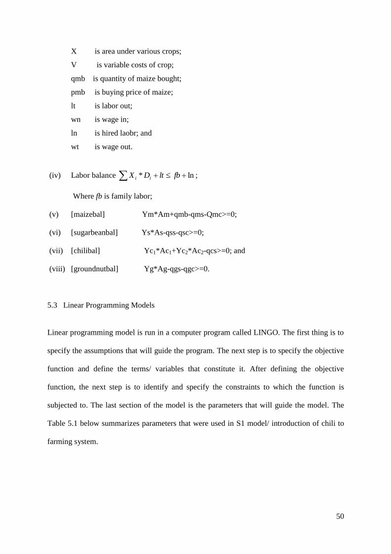
5.3 Linear Programming Models ....................................................................................... 50
5.4 Results from Linear Programming Models.................................................................. 51
5.5 Sensitivity Analysis ..................................................................................................... 53
5.6 Summary ...................................................................................................................... 55
6 DISCUSSION OF RESULTS AND POLICY RECOMMENDATIONS ..................... 57
6.1 Introduction .................................................................................................................. 57
6.2 Preliminary Analysis .................................................................................................... 57
6.3 Linear Programming Analysis ..................................................................................... 58
6.4 Policy Recommendations............................................................................................. 59
7 SUMMARY AND CONCLUSIONS .............................................................................. 62
7.1 Summary ...................................................................................................................... 62
7.2 Conclusions .................................................................................................................. 63
7.3 Limitations of the Study and Areas of Further Research ............................................. 66
REFERENCES ........................................................................................................................ 67
APPENDIX A GROSS MARGIN BUDGETS ..................................................................... 70
APPENDIX B LINEAR PROGRAMMING ANALYSIS .................................................... 74
APPENDIX C QUESTIONNAIRE ....................................................................................... 86
Page 8
viii
LIST OF TABLES
Table 4.1 Existing Cropping Pattern ................................................................................... 37
Table 4.2 Sample Distribution across Farmers’ Categories ................................................ 38
Table 4.3 Area under Chili and other Crops ........................................................................ 39
Table 4.4 Descriptive Statistics of Chili Producers. ............................................................ 40
Table 4.5 Level of Participation in Chilies with Respect to Demography .......................... 41
Table 4.6 Level of Participation with Respect to Social Characteristics ............................. 42
Table 4.7 Level of Participation with Respect to Economic Resources .............................. 43
Table 4.9 Financial Performance Indicator for Chili, Ground nuts and Sugar Beans ......... 46
Table 5.1 Summary of Parameters ....................................................................................... 51
Page 9
ix
ACRONYMS AND ABBREVIATIONS
AREX Department of Research and Extension
BRM Binary Response Model
OLS Ordinary Least Squares
FAO Food and Agricultural Organization
FGD Focus Group Discussion
GI Gross Income
GM Gross Margin
GMA Gross Margin Analysis
Kg Kilogram
LRM Linear Regression Model
MLRM Multiple Linear Regression Model
SPSS 18 Statistical Package for Social Scientist version 18
TVC Total Variable Cost
Page 10
1
CHAPTER
1 INTRODUCTION
1.1 Background Statement
Several criteria are used to come up with optimal crop/livestock enterprise mix. These range
from simple to complicated analytical tools such as gross margin budgets, cost benefit
analysis, linear programming and parametric programming. Smallholder farmers normally
depend on the knowledge about historical events in making decisions whereas commercial
farmers can sometimes use decisive complicated methods to make their decisions.
For the smallholder subsector, the difference is not only found in farm sizes but also in the
allocation of resources to food, cash crops, livestock and off-farm activities, in the use of
external inputs and hired labor, the proportion of food crops which are sold, and in the
expenditure patterns (Bijman et. al., 2007). For example, large scale commercial farmers
might want to maximize profits whereas smallholder farmers might want to maximize food
security or income or diversify risk.
The actual farming pattern, household strategies and behavior, and the livelihood pattern are
determined by resource endowments and institutional factors such as access to markets,
provision of hybrid seeds, extension and economic factors such as organization of markets
and information on prices and availability of markets. Tinsely (2004) contents that farmers
have limited education, however they are skilled practitioners of agronomy and animal
production.
The Bird’s Eye chili plant has a productive life of two to three years and can be intercropped
with herbs and spices (IDEA, 2001). Normally the seed bed is prepared in January
Page 11
2
incorporating animal manure and about 20 grams of seed which gives at least 500 good
plants. Transplanting to farmers’ fields in done late March with a recommended spacing of 1
m within rows and 1 m between rows for pure stand production. When intercropping with
other crops, the spacing has to be 2 m by 2m. Harvesting and drying commences from June
right through to August.
On well-managed farms, yields of at least 300 grams of fresh chili per plant per year or 180
grams of dried chili are expected. At a density of 10,000 plants/ha this will translate to a yield
of 1.8 tones/ha, equivalent to a cost insurance and freight (CIF) value of more than $5,000/ha
for grower-exporters as at March 1997 prices (IDEA, 2001). Harvesting is the most labor
intensive activity in chili production. Therefore it is far more profitable to harvest all the fruit
from a few plants than half of the fruit from many plants. Moreover, the need for seasonal
labor and good labor management has been a deterrent to large scale production of bird’s eye
chili (IDEA, 2001).
Kaite, a nongovernmental organization introduced chili production in Marondera and
Goromonzi Districts using organic methods in 2006. Organic farming methods reduce costs
of production and increases revenue (Firth, 2004). For example, a project which introduces
chili productions using organic fertilizer, which is cheaper, and contracts its prices and
market, guarantees income. The guaranteed price and income is likely to promote adoption of
chili production. Introduction of organic chili results in changes in relative costs of factors of
production, which induces movements in factors of production, which are land, labor and
capital. For example, we would expect land, labor and capital to move into chili production
moving away from enterprises with less return. This will lead to new optimum crop/livestock
Page 12
3
mixes. However, for the farmer to come to this new optimum enterprise mix, there are several
methods which determine pace of adoption.
Organic agriculture has become more widespread globally, as the market for certified
organic agricultural products has grown over the recent years (FAO, 2002). This has given
smallholder farmers a window of opportunity for guaranteed high value prices, and has
attracted smallholder farmers to also venture into these high value crops such as chili using
organic methods (IDEA, 2001; FAOSTAT, 2011). Organic farming has been found to be cost
effective, affordable improves liquidity management, and provides more employment
opportunities (Adhikari, 2009; Svotwa et. al., 2007). Suffer (2004) contents that organic
farming contributes directly to rural economic development. For example, through direct
sales of produce to local businesses and local community. Scialabba (2007) contents that
communal farmers can benefit from improved agro-ecological management of traditional
agriculture using low external input and inexpensive technologies such as organic farming.
1.2 Problem Statement
Smallholder farmers are characterized by low investment capacity, low resources, low
agricultural productivity and varying incomes (Mujeyi, 2007). An introduction of high value
cash crops such as chili can increase farmer’s income, food security and satisfy other
objectives (IDEA, 2000). However, any new crop diversification program will bring with it
several disturbances in terms of shifts in resource uses with resources shifting from one crop
enterprise to the other and inducement of technological changes. Introduction of a cash crop
such as chili is expected to increase household income diversification for smallholder cash
constrained farmers (Ibrahim, 2007).
Page 13
4
Kaite is a private company. It introduced chili production in the Districts of Goromonzi and
Marondera of Mashonaland-East in 2006. The project guaranteed markets and prices through
a contract. The project also provided seed and the extension services. However, when the
innovation was introduced, chili production quickly expanded because lucrative because
farmers were given inputs on credit with a guaranteed market and price. In their decision
making, farmers in the two Districts soon found out that they had to use their resources to
produce chili and other crops.
It was observed that the farmer’s crop mix had changed. Although these changes in crop mix
would be seen overtime, a priori, it could always be difficult to foretell resource movements
and technological adoption.
Kaite introduced chili production to Marondera and Goromonzi Districts with the objective of
increasing farmer’s incomes. However, a priori, no study had been done to see whether chili
production should be part of the optimum crop enterprise mix in these two Districts. The
private company however subsidized the crop by providing free seed, guaranteed markets,
free credit for inputs and extension services. The current average crop mix grown in these
two Districts is therefore a result of the current uneven resources mix. We would want to
level what would happen if the playing field was even for all crops.
1.3 Research Objectives, Questions and Hypotheses
The main objective of this thesis is therefore to estimate the optimal crop mix for an average
farmer in Marondera and Goromonzi Districts given the introduction of chili. Chilies are
produced using organic practices, marketed through a guaranteed contract which provides a
market and credit inputs. The decision of the optimal crop mix is dynamic since the decision
Page 14
5
is made repeatedly at the beginning of every season. As the socio-economic, institutional and
technical conditions change, the optimal crop and livestock enterprise mix at the farm
changes too. The study will therefore seek to satisfy the following specific objectives,
Objectives
i. Estimate average gross margin budgets for major crops grown in Goromonzi and
Marondera Districts where chili production has been introduced by Kaite;
ii. Use linear programming to estimate optimal crop mix for the average farmer in
Goromonzi and Marondera Districts; and
iii. Make policy recommendations about introduction of chilies in the production systems
of Goromonzi and Marondera Districts.
Questions
The specific objectives will be answered by asking the following questions or consistence;
i. What are the average gross margin budgets for major crops grown by farmers in
Goromonzi and Marondera Districts?
ii. What is the optimal crop mix for the average farmer in Marondera and Goromonzi
Districts and
iii. What are the policy recommendations about the introduction of chilies to the
production systems of Goromonzi and Marondera districts?
Hypothesis
In order to answer the above questions, the following null hypotheses are going to be tested;
i. The average gross margin for chili is relatively higher compared to other crops;
Page 15
6
ii. There is going to be a substitution of factors of production in favor of chili and
increase in overall income of the average farmer in Goromonzi and Marondera
Districts; and
iii. Government policy can play a role in favor of increased chili production.
1.4 Organisation of Thesis
This thesis is organised into seven chapters. The first chapter covers the introduction and
background about the issue to be studied. The main objective of the thesis is to estimate the
optimal crop mix for an average farmer in Goromonzi and Marondera Distircts,
Mashonaland-East.
The second chapter provides literature review. The literature reviews the theory of production
and resource allocation in smallholder farming systems. The review also looks at adoption
process of new technologies. The chapter also provides an overview of factors influencing
chili production in Zimbabwe as well as empirical tools commonly used in estimating
optimal crop mix in farming system.
The third chapter provides an outline of the research methods used in the study. The study
used gross margin budget analysis and linear programming to estimate the optimal crop mix.
Chapter 4 provided the preliminary analysis of the research data. The analysis tests the first
hypothesis and finds out that indeed chili production had the highest gross margin of US$380
given US$129 for maize, US$349 for ground nuts and US$180 for sugar beans.
Chapter 5 estimates the optimal crop mix for an average farmer in Goromonzi and Marondera
Districts in 2010. The chapter also provides some sensitivity analysis at 5% and 10%
Page 16
7
changes. Sensitivity analysis shows that land moved to chili with increase in land brought
under production. Chapter 6 contains the discussion of the results found in chapter 4 and 5
and policy recommendations. Chapter 7 provides conclusion.
Page 17
8
CHAPTER
2 LITERATURE REVIEW
2.1 Introduction
The main objective of this chapter is to provide a detailed literature review on the economics
of crop production, evaluate factors influencing crop production, evaluate methods used in
similar studies on the economics of crop production, and get insights on theoretical and
policy issues, and other issues surrounding crop production. The chapter starts by reviewing
the economics of crop production, focusing on the production theory and using chili
production in Goromonzi and Marondera Districts as examples. Production theory defines
output or production as a function of several inputs, such as land, labour, capital and
management (Oluwatayo et al., 2008). These factors of production can be both varied or
fixed depending on the time frame, that is short run, medium run or long run, and depending
on space, that is, extensive or intensive, particularly in Zimbabwe.
The major factors or inputs or resources which influence production are land, labour, capital
and management (Binam et al., 2004; Sojkova et al., 2007). The level of education of the
household head, farming experience, frequency of extension visits and access to credit have
an impact on economic efficiency in production. Increase in human capital enhances
productivity because farmers are better able to allocate labor and purchased inputs. It also
enhances farmer’s ability to receive and understand information relating to new technology.
The section further analyses the relationship between factors of production and production.
Farmers with more years in school, have access to credit, and are members of associations
have increased productivity.
Page 18
9
The chapter further looks at research methods which have been used in the literature to
determine optimum crop or enterprise mix on the farm. Every farmer is faced with a problem
of deciding the enterprise mix during the beginning of every season, and by so doing
allocating the scarce resources available to him (Sirohi et al., 1968). There are several
methods in the decision making process starting from rudimentary methods, historical
experiences to sophisticated methods such as cost benefit analysis, gross margin budget
analysis, linear programming, nonlinear programming and other decision making methods.
Finally, the chapter discusses about the experiences of policy implications emerging from
these studies and areas for further research and insights into the evaluation process.
2.2 The Economics of Crop Production
Production is the processes and methods employed to transform tangible factors/ resources or
inputs namely raw materials, semi-finished goods; or sub-assemblies, and tangible inputs
such as ideas, information and knowledge into goods and services or output (Oluwatayo et.
al., 2008). These resources can be organized into a farm-firm or producing unit whose
ultimate objectives maybe profit maximization, output maximization, cost minimization or
utility maximization or a combination of these objectives four. In this production process the
manager or entrepreneur may be concerned with efficiency in the use of the factor inputs to
achieve optimum crop mix.
The basic theory of production is thus simply an application of constrained optimization. The
farm-unit attempts either to minimize the costs of producing a given level of output or
maximize output attainable with a given level of costs (Oluwatayo et. al., 2008). Both
optimization problems lead to the same rule for the allocation of inputs and choice of
technology. Since there are alternative means of attaining the production goals, the theory of
Page 19
10
production presents the theoretical and empirical framework that facilitates a proper selection
among alternatives so that any one or a combination of farmer’s objectives can be attained.
Certain parameters have to be known for one to understand how farmers make their decisions
that enable them to attain their goals. These parameters can be shown through a production
function, which shows the technical relationship between factor inputs and outputs involved
in the production process. The basic assumptions of production function are presented in two
graphs. The first represents output as a function of input and introduces the three stages of
production Let y = output and x = input. The production function is y = f(x); marginal
productivity (MP) is fx =δf/δx; and average product (AP) is y/x. Recall that
MP > AP > 0; at Stage I of production function
AP >MP >= 0; at Stage II of Production function, and
MP < 0; at Stage III of production function
The second stage is the economic region. This is the stage with positive but decreasing
marginal productivity or concave production function. A competitive profit maximizing firm
is likely to operate at this stage of the production function. Many mathematical specifications
of production functions, like for example the Cobb-Douglas: y = Axɑ, with 0 < ɑ < 1, only
represent situations when all outcomes are at the economic regions. Their use precludes
identifying situations in which producers operate at the third stage of production and have
negative marginal productivity. Quadratic production functions, y = ɑ + bx - cx2, allow
outcomes at the second and third regions of production functions, but not at the first. A
simple and elegant production function which allows three regions of production is not easy
Page 20
11
to construct, so we use simple, elegant but flawed production function specifications in many
analyses.
Output y
Stage 1 Stage2 Stage 3
0 Input, x
Figure 2.1: Three stages of Production
Source: Sojkova et al., 2007
Figure 2.1 addresses the relationships between output and input in the production process. A
basic issue it raises is that of economies of scale. It represents the assumption that below a
certain level of output (stage 1), there is increasing returns to scale. However, at the economic
region, there is constant, or more likely decreasing returns to scale.
Figure 2.2 represents the relationship between inputs in the production process. The isoquants
depicted represents the different input level combinations producing the same level of output.
Isoquants are useful to address issues such as input intensity and input substitutability. If X1
is capital and X2 is labor, X1/X2 measures capital intensity (relative to labor). Production at
point A is capital intensive and at B is labor intensive.
Page 21
12
Capital,X1 Y=Y1>Y0
Y=Y0 KA/LA
KB/LB
A B
0- Labor, X2
Figure 2.2: Isoquants and Factor intensity
Source: Sojkova et al., 2007
Based on neo-classical production theory, the dependent variable of the production function
should be expressed as the quantity of a given output produced in a given time period as a
result of a production transformation of a given input quantity (Sojkova et. al., 2007). This
definition is followed by the first endogenous variable specification of the stochastic frontier
production model, namely the output is the amount of a produced commodity in a farm (farm
enterprises production), expressed in tons.
By using this production definition, we assume that the production quantity is homogenous
when comparing the analyzed enterprises. Constructing a production function requires further
information about inputs equipment in quantity references. Because only cost data is
available for production factors, no breakdown between quantity and prices is possible. The
agricultural production process is a complex activity where not only inputs quantity, but also
input quality and functionality have a significant impact on input performance (Oluwatayo et
al., 2008).
Page 22
13
2.3 Factors Influencing Crop Production
Nyagaka et al., (2009) did a study on economic efficiency of potato production in Kenya and
found out that the level of education of the household head, experience, number of extension
visits, and access to credit are significant variables for improving the level of economic
efficiency of potato production. The positive impact of education on economic efficiency
indicates that increase in human capital will enhance the farmer’s ability to receive and
understand information relating to new agricultural technology. This finding supports
argument by several authors that an increase in human capital will augment the productivity
of farmers since they will be better able to allocate family-supplied and purchased inputs,
select the appropriate quantities of purchased inputs and choose among available techniques
(Sirohi et al., 1968; Binam et al., 2004).
A study by Nyagaka et al., (2009) revealed that economic efficiency increases with the
number of years spent in potato production by the household head. This suggests that farming
is highly dependent on the experience of farmers which may lead to better managerial skills
being acquired over time. Farm households who receive regular extension visits by extension
workers are more economically efficient than their counterparts. Thus economic efficiency
increases with the number of visits made to the farm household by extension workers. Nchare
(2007) supports this argument when he indicated that regular contact with extension workers
facilitates practical use of modern techniques and adoption of improved agronomic
production practices.
Farmers with access to credit tend to exhibit higher levels of economic efficiency and are
able to better allocate their limited resources among competing alternatives (Nyagaka et al.,
2009). So access to credit permits a farmer to enhance production by overcoming these
Page 23
14
liquidity constraints. Liquidity constraints may affect farmer’s ability to apply inputs and
implement farm management decisions on time. The use of credit therefore ensures timely
acquisition and use of inputs and results in increased economic efficiency. Binam et al.,
(2004) used farm-specific variables to explain technical inefficiencies. Their results revealed
that those farmers who have more than four years of schooling, better access to credit, located
in fertile regions and those who are members to farmers’ club or association tend to be more
efficient. The distance of the plot from the main access road and the extension services have a
negative influence in increasing technical efficiency in different farming systems (Binam et
al., 2004).
Sojkova et al., (2007) used four inputs variables and one output of the stochastic frontier
production models for the analysis of Slovak farm enterprises: capital, labor, material and
agricultural land as inputs and total production as the output. However, under organic
systems crops rely on ecologically based practices, such as biological pest management and
composting, and the exclusion of synthetic chemicals. The fundamental components and
natural processes of ecosystems such as soil organism activities, nutrient cycling, and species
distribution and competition are used as farm management tools (McBride et al., 2008). For
example, crops are rotated, food and shelter are provided for the predators and parasites of
crop pests, animal manure and crop residues are cycled and planting/ harvesting dates are
carefully timed.
The role of social capital in providing incentives for efficient production is revealed by the
negative and statistically significant relationship between club membership of a household
member and technical inefficiency in Binam et al., (2004). Farmers that are club members
can be very valuable for small-scale operations, because it facilitates access to markets and
Page 24
15
increases income and employment for growers. In addition club members provide farmers
with a secure market for their crops as well as some technical assistance: source of farmer
technical efficiency. A study done by Ibrahim et al., (2010) using a partial budgeting analysis
for the alternative Striga control revealed that the costs of fertilizer and labor accounted for a
substantial part of the total costs of the five treatments. Fertilizer cost ranged between 38-
54% while labor cost ranged between 41% and 55% across the five treatments respectively.
Linear regression analysis revealed that all variables in the model had positive regression
coefficient indicating direct relationship between each of them and the output of maize (Onuk
et al., 2010).
Labor inputs by household members are often higher in cash than food crops. The income
and nutritional effects of shifts from subsistence to commercialized crop production may be
highly time and place-specific, as a review of some evaluations of cash cropping schemes has
indicated (Immink et. al., 1991). The broad findings of these studies indicate that a shift
towards commercialized crop production such as chili involves significant reallocation and
increased productivity of household resources, particularly land and labor, and is associated
with significant increases in household income.
2.4 Research Methods for Evaluating the Economics of Crop Production
The use of gross margins became widespread in the UK from about 1960, when it was first
popularized amongst farm management advisers for analysis and planning purposes (Firth,
2011). The gross margin per hectare or per head for crops and livestock can be compared
with ‘standards’, published averages of what might be typically possible in average
conditions) obtained from other farms. Gross margins, however, should only be compared
with figures from farms with similar characteristics and production systems. With this
Page 25
16
reservation in mind, the comparisons can give a useful indication of the production and
economic efficiency of an enterprise. In organic systems gross margins are also useful for
farm planning and for making comparisons of enterprises, on the same farm, between organic
holdings, or between conventional and organic enterprises holdings (Firth, 2011).
Gross Margin Analysis (GMA) provides a more convenient and simple way to summarize
information required in determining the financial performance of a farm enterprise. Onuk et.
al., (2010) did an economic analysis using gross margin and the results revealed that maize
has established itself as a very significant component in the smallholder farming system of
Nigeria and is determining the cropping pattern of the farmers. IDEA, (2001) used gross
margins to evaluate performance of chili in smallholder farmers and found them to be
profitable because of the low investment costs. Expenses incurred were for seeds, land
cultivation, fertilizers, chemicals, labor and processing.
Ebukiba (2010) did a study to evaluate the economic analysis of cassava production in Eket
local government area of Akwa Ibom State of Nigeria using gross margin analysis. Gross
Margin Analysis was used to analyze the cost and return data, the result reveals that for a
hectare of sole cassava the gross margin was N141,950 giving a cost benefit ratio of N1.90;
N1.00 implying that cassava production is profitable. Ibrahim et. al., (2010) conducted a
study to compare economic performance of five Striga control methods in Nigeria using
gross margin analysis. The results revealed that treatment plots involving the cultivation of
Striga tolerant maize variety followed by Striga tolerant maize variety in the second year
(T1) had a higher cumulative gross margin per hectare (N76, 884.61) followed by the
treatment involving the cultivation of an improved soya bean variety (TGX 1448-2E)
followed by Striga tolerant maize variety in the second year i.e.T2 (N36, 287.00). The
Page 26
17
marginal rate of return was also higher for T1 (N885.00) followed by T2 (N8.90) (Ebukiba,
2010).
Ranadhawa et. al., (1966) applied inter-regional programming model to determine an optimal
allocation of land among different crops and regions of India. They used gross returns to
develop optimal production pattern but found that it would be better if net returns were used
in the analysis. They also pointed that cash costs in their study formed a small proportion of
the total cost and then reported that the situation had changed and the proportion of variable
cost to the total cost had increased and the concept of gross returns seemed to have lost its
relevance (Ranadhawa et al., 1966).
Papst et al., (1970) used linear programming technique to develop farm plans for a 470-acre
model farm in Mason County, Illinois. The results showed that the farm plans gave the
highest net return above variable costs for each of four basic situations: no irrigation, 150
acres irrigated, 287 acres irrigated, and 437 acres irrigated. The highest return plans were
found to be relatively insensitive to changes in relative prices and yields. There was a
declining rate of return on added investment in irrigation equipment as the area irrigated
increased; the rate of return on equipment to irrigate the first 150 acres was 37 percent, while
the rate of return on the added investment necessary to irrigate 150 additional acres from a
base of 287 acres was only 7 percent.
Ibrahim (2007) did a study to determine the optimal maize-based enterprise in soba local
government area of Kaduna state, Nigeria. The linear programming analysis indicated that a
gross margin of N56, 920,30 was obtained in the planned farm as against N26,282.00, per
hectare of maize/cowpea in the unplanned farm. Curtis et al., (2009) used data on current and
Page 27
18
alternative crops such as enterprise budgets, producer interviews and field trials in North
Western Nevada USA. They used an EPIC Model which synthesizes both agronomics and
economics, to model yields and returns of alternative crops under differing irrigation levels.
This study determined that the alternative crops that could be feasibly substituted for alfa
alfa and reduce water use by half while providing net returns that meet or exceed returns from
alfa alfa and keep producers profitable.
Cashdollar (1971) used linear programming analysis to determine the most profitable crops
grown on representative farms under two sets of localization regulations for the Fortieth
Distributary in Mysore state, India. The results showed that in situations of limited operating
capital, the dry land crops compete favorably with irrigated crops, primarily because of the
higher returns per rupee invested in cash inputs on the dry land crops. It was found that paddy
competes favourably with the light irrigated crops where developed land and capital are
plentiful. However, when developed land is limited it is generally more profitable to double
crop with two light irrigated short duration crops than to grow one crop of longer duration
paddy.
Sirohi et al., (1968) assessed the possibility of increasing net farm returns through
reorganization of resources by employing linear programming. The results of their study
showed that by reallocation of resources, net farm returns could be increased to the extent of
24 to 42 per cent. Singh (1970) used linear programming technique to know the possibilities
of increasing the income and labor absorption through optimal combinations of crop and
dairy enterprises. He developed optimum plans under existing as well as improved
technology with limited and unlimited capital. He concluded that inclusion of dairy was
profitable with both the limited and unlimited capital situation.
Page 28
19
Linear programming techniques were employed to assess the impact of dairy enterprise on
productivity and employment by Singh et al., (1977). They concluded that the normative
plans developed with and without dairy not only affected the productivity and employment
but also the requirements of capital and credit on the farms. The capital and credit
requirements increased with the dairy activity. It was also found in the optimum plans, two
buffaloes for small; three for medium and eight for large farmers to be necessary to maximize
their net farm returns. Singh et al., (1977) used a similar technique to study the impact of
varying levels of dairy enterprise with crop farming on income and employment. They
concluded that the farm income and labour use could be increased through optimization of
resource use under different farm situations.
To develop optimum farm plans for subsistence and commercial farmers in Bangalore
District, a linear programming technique was applied by Ramanna, (1966). He reported that a
substantial increase in net farm returns could be realized by proper reorganization of
available resources even with the available technology. He also pointed out the prospects of
higher net farm returns under improved technology with additional resources. Nadda et al.
(1978) explored the possibilities of optimizing farm returns for the farmers of different zones
in Himachal Pradesh. They concluded that existing cropping pattern where diversification of
agriculture observed was found sub-optimal. The normative cropping pattern involved fewer
crops, indicating a tendency towards specialization.
The impact of optimal allocation of supervised production credit on different farm size
groups was assessed by employing linear programming by Arora et al., (1978). The results
revealed that the gains of optimal credit allocation were more on small farms followed by
medium and large farms. Thore et al., (1985) used linear programming to study the impact of
Page 29
20
dairy enterprise on costs and returns and concluded that mixed farming with dairy had a
positive effect on the income of the farmers in all the size groups. Singh et al., (1988)
employed linear programming to integrate improved technology of crop and dairy production
for increasing income and employment. They concluded that the optimization of resources
under different farm plans resulted in increased income on marginal, small, medium and large
farms. Adoption of improved technology in both the crop and dairy production increased the
income of the farmers by 116 per cent for small farmer to 232 per cent for marginal farmers
as compared to the existing plan.
Sastry (1993) applied linear programming to develop optimum enterprise system for farmers
in Chittoor District, Andhra Pradesh. They indicated greater scope for increasing the net farm
income on small farms by mere reorganization of resources even under existing technology
with available funds. Further, they found that the effect of optimization of resources at
existing technology, both under restricted and unrestricted capital was insignificant on large
farms. Lakshmi, (1995) used linear programming to determine the income and employment
prospects of farmers in Chandragiri Mandal of Chittoor District. The study indicated that the
simultaneous provision of credit and adoption of new technology would enhance the income
and employment opportunities on small and large farms.
By using linear programming technique, another author developed optimum crop and dairy
mix for farmers in Bangalore district in India (Reddy, 1979). The results of the study
indicated one cross bred cow for small farmers, one cross bred cow and one local buffalo for
medium farmers and none for large farmers in normative plans of crop and dairy mix. As a
result the net farm returns increased by 45.77 per cent for small, 42.25 per cent for medium
Page 30
21
and 57.88 per cent of large farmers over existing plan. He concluded that the introduction of
dairy along with crops would be more profitable only in case of small and medium farmers.
Reddy, (1980) employed linear programming tool to examine the income and employment
potential on small farms in Bangalore district, Karnataka. It was observed that the net farm
return increased to the extent of 50 and 16 per cent on unirrigated and irrigated small farms
respectively by mere reallocation of resources at existing technology. The results also
indicated the prospects of raising the income by 110 per cent on unirrigated farms and, by
14 per cent on irrigated farms, when capital constraint is relaxed. Singh et al. (1972) in their
study on production possibilities and resource use pattern on small farms in three regions of
Uttar Pradesh examined the prospects of increasing farm income through better resource
allocation. It was observed that the farm resources were not utilized optimally under existing
cropping pattern and reorganization of production programme would increase the farm
income even under the existing resource availability.
2.5 Lessons Learnt from the Literature Review
Increase in human capital leads to increased productivity since farmers will better allocate
their resources and choose among available resources. Farmers acquire better managerial
skills over time thus farming is highly dependent on experience of farmers. Frequency of
extension contact has a positive effect on adoption of improved techniques and their practical
use (Nyagaka et al., 2009). Availability of credit eliminates liquidity constraints hence
increasing farmer’s ability to apply inputs and implement farm decisions on time. Social
capital plays a significant role in increasing productivity of the farmer. Farmer associations
facilitate access to markets resulting in increase in income for its members. It also provides
secure markets for crops as well as technical assistance (Binam et al., 2004).
Page 31
22
Firth, (2011) noted that gross margin should be compared with figures from farms with
similar characteristics and production systems. Moreover, gross margin analysis is useful for
farm planning and for making comparisons of enterprises on the same farm and for
determining the financial performance of a farm enterprise. Ranadhawa e. al., (1966) reported
that gross returns lost its relevance in a study they did to determine an optimal allocation of
land among different crops and regions. They concluded that use of net returns provides
better results in developing optimal production patterns.
Regardless of its convenience and simplicity, GMA has its own limitations. Gross margins do
not tell whether a particular way of producing an enterprise is optimal, most profitable, or
best way of producing that crop. They only tell about net returns on resources employed in
producing the crop. Positive gross margin values do not necessarily mean that the enterprise
is technically efficient in producing the crop. It is very difficult to tell, with a GMA, why an
enterprise might have positive margins but fail to attract satisfactory investment by farmers
(adoption) in terms of resource allocation. Finally, GMA fails to take into account potential
social and environmental impacts as a result of implementing activities of the production
enterprise. Such impacts can be considered by assigning values to the social and
environmental benefits, costs and including them, in the GMA. These benefits and costs are
usually not included due to difficulties in measuring and computing them.
Kahlon et. al., (1962) in their study on the application of budgeting and linear programming
in farm management analysis reported that linear programming might be preferred where the
choice was to be made among many alternatives and high accuracy needed, that enabled even
a less skilled worker to reach an optimum solution. Therefore, linear programming is
Page 32
23
considered a useful tool of farm management analysis even in under developed countries.
These findings have much support from other writers who stated that the linear programming
offers a great scope for its usage with advantage and even alternative plans could be worked
out for different prices (Desai, 1962; Malya, 1962; Ramanna, 1966). They concluded that the
pressing need for reorganization of the limited resources made the application of linear
programming, a necessary step towards efficient farm business management.
2.6 Conclusion
The objective of this chapter was to carry out a detailed literature review on the economics of
crop production and the methods that have been used in empirical studies to decide on
optimal crop mix. This critical decision is made by each farmer at the beginning of the season
using several methods. The chapter starts by describing duality in economics of production,
that is maximizing profits leading to the same decision rule as minimizing costs of
production. The production theory defines output or production as a function of several inputs
such as land, labour, capital and management. These factors of production can be both varied
or fixed depending on the time frame, that is short-run, medium-run or long-run, and
depending on space, that is, extensive or intensive particularly in Zimbabwe.
The chapter further looks at factors influencing production and household resource
allocation. The major factors or inputs or resources which influence production are land,
labor, capital and management. The level of education of the household head, farming
experience, frequencies of extension visits and access to credit also affects production.
Increase in human capital enhances productivity since farmers are better able to allocate labor
and purchased inputs, and it also enhances farmer’s ability to receive and understand
information relating to new technology. The section further analyzed the relationship between
Page 33
24
factors of production and production. Farmers with more years in school have access to credit
and have membership of association have increased productivity
There are several research methods that have been identified in the literature. The methods
reviewed varied from gross margin to linear programming models. Gross margin analysis is
useful for farm planning, for making comparisons of enterprises on the same farm and
determining the financial performance of a farm enterprise. Linear programming has been
used in crop-livestock enterprise mixes to explore possibilities of increasing income and labor
absorption through optimal combinations.
Further, the chapter reviewed the empirical studies that have been done to estimate optimal
crop/enterprise mix at farm level. Linear programming has been used by several authors to
develop optimum enterprise systems on farms. The results showed that net farm income can
be increased by reorganization of resources under existing technologies and funds. There are
prospects of higher net farm returns under improved technologies with additional resources.
Finally, the chapter looked at the lessons learnt from the literature review. The impact on
each factor depended on place and space. Regular extension contact facilitates adoption and
practical use of improved production technologies. It is very difficult to tell with GMA, why
an enterprise might have positive margins but fail to attract satisfactory investment by
farmers in terms of resource allocation. Gross Margin Analysis has weakness. Linear
programming has weakness also, so it is better to use both methods. The pressing need of
reorganization of the limited resources made the application of linear programming a
necessary step towards efficient farm business management.
Page 34
25
CHAPTER
3 RESEARCH METHODS
3.1 Introduction
Chapter 3 presents research methods. The chapter provides the conceptual framework that
will be used in showing the different relationships between the economic variables and the
analytical framework that will be used to analyze the data set, and present the expected
results from the theoretical model. The chapter starts by describing the conceptual framework
that has been developed for this thesis. The conceptual framework relates different concepts
from theory to show the relationships between different economic variables. For example,
introduction of a new enterprise affect resource allocation as farmers shift some of the
resource to accommodate the new enterprise.
The chapter further looks at the analytical framework that will be employed in analyzing the
data. Gross Margin Analysis is an input into linear programming analysis. It is an analytical
tool used in financial analysis to determine performance of agricultural enterprises. However,
gross margin is not a decision tool because increases in margin will also results in increase in
the relative costs. Thus at any particular gross margin there is a corresponding cost structure.
Results of gross margin analysis are further used in linear programming analysis to estimate
the optimal enterprise mix at farm level.
Finally, the chapter presents the expected results from the theoretical model. Average gross
margin for chili is relatively high compared to other crops. Chili uses minimum purchased
resources, variable costs associated with the production of the crop will be low compared to
Page 35
26
other crops hence a higher and positive gross margin since production is subsidized.
Substitution of land use in favor of chili production and increase in overall income of the
farmer is expected. Finally, linear programming analysis in next chapter will test the optimal
mix given introduction of chili in the production system in Goromonzi and Marondera
Districts.
3.2 Conceptual Framework
An optimum crop mix is situation where a farmer’s objective is to maximize gross income
given some level of resource. Introduction of chili redistributes resource allocation and crop
mixes for the farmers. In the process it is expected that it enhances income, creates
employment and method of production is cost effective especially for rural communities
(Ranadhawa et al., 1966).
Chili production has proved to be a worthwhile enterprise for smallholder farmers in
developing countries such as Uganda (IDEA, 2001). Inputs such as fertilizers, seed, land,
manure, pesticides have been used to produce chili. However, the production system has been
influenced by chili characteristic among other factors such as organic practices being
employed, farmer’s characteristics such as sex, experience in chili farming, and education of
household and resource endowment (Sirohi et al., 1968). All these factors determine the
quality and quantity of chili being produced by the farmer, hence the profit margin that can
be realized by the farmer. Chili with a high pungency and are red receive premium prices on
the market. The production method used in producing the chili of employing organic methods
is highly labor intensive and this has an effect on the variable costs as labor costs are very
high relative to other costs (IDEA, 2001).
Page 36
27
Choice of and participation in chili production is influenced by the farmers’ access to social,
economic and financial resources such as land, labour, capital and frequency of access to
extension. An enterprise might have a favourable gross margin but farmers will still be
reluctant to adopt/ reallocate resources towards it (Ebukiba, 2010).
Optimum farm plans for smallholder farmers can be achieved by employing a linear
programming technique. Substantial increase in net farm returns could be realized by proper
reorganization of available resources even with the available technology. There are even
prospects of higher net farm returns under improved technology with additional resources.
Simultaneous provision of credit and adoption of new technology would enhance the income
and employment opportunities on small and large farms.
3.3 Analytical Framework
The study employs two frameworks in analyzing the specific data set. The first one is the
gross margin analysis (GMA), and the second one is the linear programming model (Onuk et
al., 2010); IDEA 2001). The gross margin analysis is the difference between the value of
gross output and total variable costs per unit of a resource, usually a hectare of land for a
particular enterprise. It is the most common analytical tool used in financial analysis for
determining performance of agricultural enterprises and projects (Onuk et. al., 2010;
Ebukiba, 2010). The financial performance of enterprises is determined at the market prices
by taking account of different input usages and values of outputs. The GMA was chosen
because of its simplicity.
To conduct a gross margin analysis for a farm enterprise, a physical budget of the enterprise
is transformed into financial terms by attaching costs and prices to each item of the budget.
Page 37
28
GM is simple in the sense that it does not consider fixed costs, which are often difficult to
compute and allocate to individual enterprises. Following Ebukiba, (2010) GM is specified as
follows,
N
i
ii
N
i
ii TVCQPGM11
*
Where,
GM = Gross Margin (US$/acre);
TVCi = Total Variable Cost (US$/acre) of the ith
enterprise;
GM is the difference between income and variable costs;
Gross Income (GI) = Pi*Qi ;
Pi is price per unit of out of a certain enterprise i; and
Qi total quantity produced by the ith
enterprise.
Total variable costs (TVC) are the direct costs incurred in producing the output. These costs
among others include fertilizers, seed, casual labor, land cultivation and processing (IDEA,
2001). Gross margin is not a decision rule tool because increase in the margin will also
results in increase in the relative costs, thus at any particular gross margin there is a
corresponding cost structure (Ebukiba, 2010). The results of the gross margin analysis are
used in the linear programming model for further analysis. Further economic analyses, for
example included estimation of optimal crop mix that will maximize farm income.
With given physical, technical and resource conditions, optimal allocation of resources
entails the efficient use of each resource such that the net farm returns are maximized in a
year (Cashdollar, 1971). Among the various analytical tools available for allocation of
available but limited farm resources, linear programming is one of the most widely and best
Page 38
29
understood operations research techniques (Ramanna, 1966). It is indeed a powerful
technique, which can effectively handle large number of linear constraints and variables or
activities simultaneously. Linear programming technique is a useful tool to estimate optimal
crop mix of designate form under varied capital and technological environments.
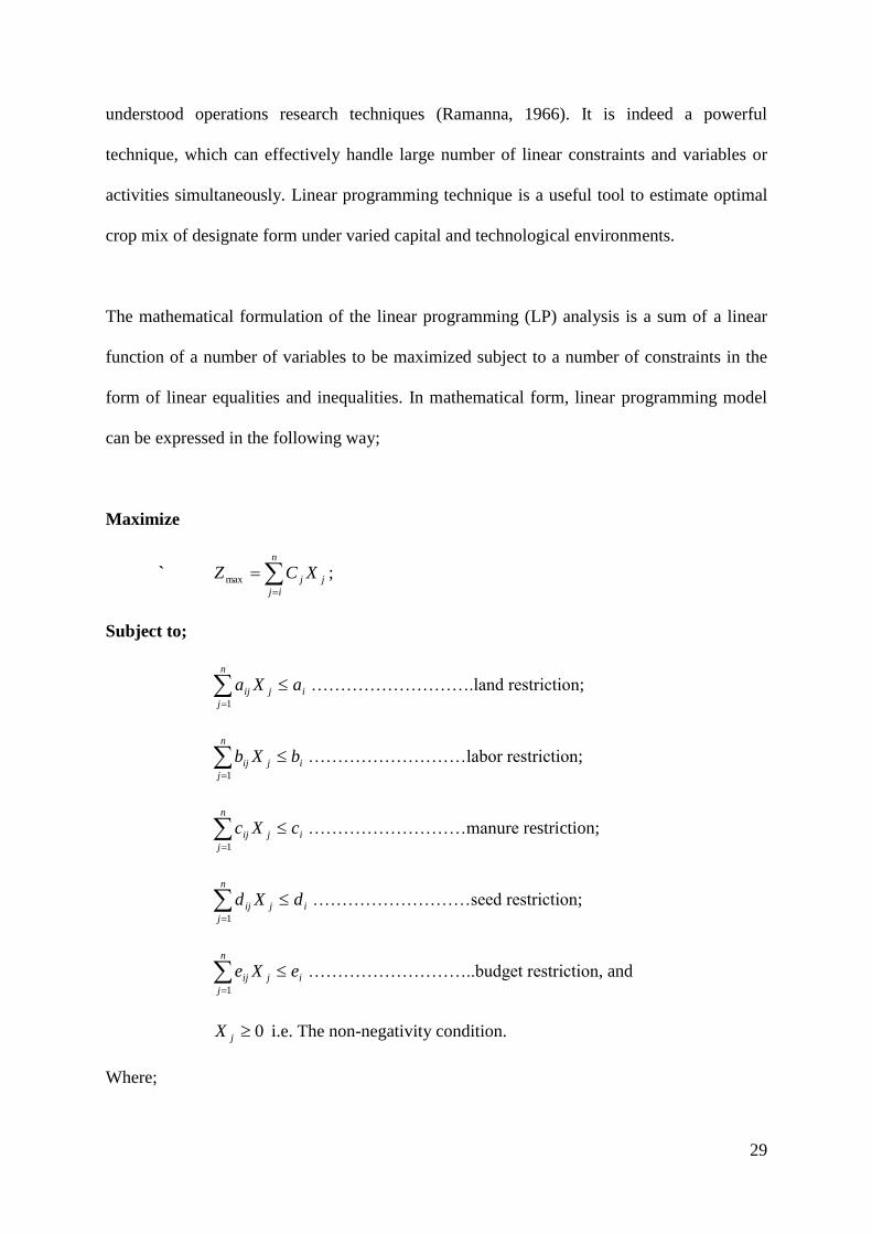
The mathematical formulation of the linear programming (LP) analysis is a sum of a linear
function of a number of variables to be maximized subject to a number of constraints in the
form of linear equalities and inequalities. In mathematical form, linear programming model
can be expressed in the following way;
Maximize
` j
n
ij
j XCZ
max ;
Subject to;
n
j
ijij aXa1
……………………….land restriction;
n
j
ijij bXb1
………………………labor restriction;
n
j
ijij cXc1
………………………manure restriction;
n
j
ijij dXd1
………………………seed restriction;
n
j
ijij eXe1
………………………..budget restriction, and
0jX i.e. The non-negativity condition.
Where;
Page 39
30
Z = Objective Function;
Xj = area under jth crop production activity;
Cj = Gross margin per unit of the jth crop activity;
aij= land coefficient for jth crop;
bij = labour requirement for jth crop activity;
cij = manure requirement for jth crop activity;
dij = seed requirement for jth crop activity;
eij = budget requirements for the jth crop activity;
ai =available land in acres;
bi =human labour available in man-hours;
ci =available manure in Kg;
di =quantity of seed available in Kg;
ei = amount of money available; and
n =Number of crop production activities.
The LP model starts by assuming an objective function. The objective function consists of the
income generating activities which are crop production and or livestock activities. It is
assumed that the farmers' objective is to maximize net returns that is a product term of
average yield of an enterprise and its unit price to family labor, land, management, and
capital invested in the crop enterprises. The linear program is run for maximization of net
returns. Linear programming model maximizes income on a representative farm subject to
the resource limitations as reflected by resource availabilities on the farms.
In order to run LP model, several basic assumptions are made. For example, besides the
general assumptions of linearity, divisibly, non-negativity, additivity, finiteness and certainty,
several other potential assumptions are made in developing the model (Varalakshmi, 2007).
Page 40
31
In this study, the problem of resource optimization was dealt at the average farm level. Each
farm was assumed to be an economic decision making unit. The farm operator was free to
make decision regarding the business limited only by legal and contractual arrangements. It
was also assumed that each farm was operated with the objective of maximizing net farm
returns subject to the described constraints only. Closely related to the above assumptions,
the study, to start with, was in static framework. It was assumed that the input and product
markets were perfectly competitive, and yield and price expectations of the farmers were
single valued.
The model had several restrictions. For example, the row vector in the matrix refers to the
constraints in the model. The different types of constraints included in the model were
physical resource constraints, product constraints, minimum and maximum area constraints
and financial constraints. The model has also resource constraints. There are several resource
constraints, for example, land restriction. Besides land, labor is also a limiting factor. Labor
could be hired or use of family labor. Farm yard manure and compost were also used as
inputs/ factors of production and their limited availability provides limitations to the model.
Finally, the output/product provides limitations to the model. It facilitates the allocation of
crop products produced between consumption and marketing. Production inventory at the
beginning of the farm operation is supplemented by output from the crop production
activities. Family consumption requirement ensures that the minimum requirement of the
household is met from the farm itself. The response of the farmers on their minimum
requirements of farm products is used to account this constraint.
Page 41
32
Further, finances are also a resource limitation imposed due to cash availability. The working
capital availability with farmers sometimes may not be sufficient to meet the requirements of
different agricultural operations. Nevertheless, it may also limit the scope for adoption of
improved production practices. Factors like risk, uncertainties, high input costs, and
supervision and marketing problems associated with certain enterprises may prevent the
farmers from taking up these enterprises beyond certain limits. While allocating the
resources, it becomes all the more important to see that the resources allocated to these
enterprises do not go beyond the limits set by the farmers. Hence, maximum area that could
be brought under high yielding and more profitable crops was specified based on the
responses of the sample farmers.
3.4 Expectations of the Theoretical LP Model
Gross margin analysis is used to give information about the performance of each crop in the
LP model. Inputs such as land, labor, capital, and other production costs variables are
factored into the model to give total variable cost. Positive margins are expected after less the
total variable costs from gross income for chili and other crops. A positive gross margin is
expected which implies that the crop is performing well, and can be incorporated into the
crop mix on the farm. Average gross margin for chili is expected to be relatively higher than
the other major crops grown in the two Districts. However, information from gross margin
alone will not help in estimating the optimal crop mix; hence the information is then used in
informing linear programming for the estimation of the optimal crop mix.
Linear programming is used to determine the optimal combination of maize, groundnuts, chili
and sugar beans to produce and sell to maximise profits. It is every farming household’s goal
Page 42
33
to maximise profits. In the process of maximizing income, substitution and reallocation of
resources will take. There is going to be a substitution of factors of production in favor of
chili and increase in overall income of the average farmer in Goromonzi and Marondera
Districts and government policy can play a role in favor of increased chili production
3.5 Conclusion
Chapter 3 presented the research methods which were going to be used to achieve my
objectives. The first section looked at the conceptual framework. The conceptual framework
discussed the conceptualization of the economic relationships in the study. Introduction of a
new enterprise affected resource allocation as farmers re-organized resource use to
accommodate new enterprise and increase income.
The second section looked at the analytical framework that has been used to estimate optimal
crop mix on the average farm. Gross margin is not a decision tool because increase in margin
will also results in increase in relative costs, thus at any particular gross margin there is a
corresponding cost structure. The gross margin analysis determines the financial performance
of the enterprise and it informs linear programming analysis. Linear programming analysis
handles large number of variables and constraints simultaneously. the method estimates
optimal crop mix under smallholder or large scale farming conditions.
Finally, the last section looked at results expected from the study. It was hypothesized that
average gross margin for chili is relatively high compared to other crops, and thus there is
going to be substitution of land use in favor of chili. To achieve my objectives, the following
chapters will analyze the research data. The research data was collected from a field survey
using a questionnaire in Goromonzi and Marondera Districts.
Page 43
34
CHAPTER
4 PRELIMINARY ANALYSIS
4.1 Introduction
The main objective of the study is to estimate the optimal crop mix for an average farmer in
Goromonzi and Marondera Districts given the introduction of chilies. The chapter starts by
providing sampling methods, data collection and data management to produce socio-
economic characteristics of farmers in Goromonzi and Marondera Districts. The chapter
further looks at the socioeconomic characteristics of smallholder farmers in the communal
farming areas of Goromonzi and Marondera Districts where organic chili production is taking
place. The chapter further presents the gross margin budgets for major crops grown in the
areas.
Finally, the chapter estimates average gross margin budgets for major crops grown in
Goromonzi and Marondera Districts where chili production has been introduced by Kaite.
The analysis will test the first hypothesis that chili has the highest gross margin relative to
other crops grown by farmers. The hypothesis is answered using gross margin created in
Excel Program. Gross margin is the difference between gross income and total variable costs
of undertaking activities of the enterprise. It is a simple indicator of performance of an
enterprise. It does not measure a crop's profitability.
4.2 Sampling Procedure, Data Collection and Data Management
The study was carried out in Goromonzi and Marondera Districts in Zimbabwe’s
Mashonaland East Province. Goromonzi and Marondera Districts are in agro-ecological
Page 44
35
region 2b, a semi-intensive farming region with annual rainfall of 750-1000mm. The
vegetation is mainly ‘mutondo’ woodland on predominantly sandy loam soils of low inherent
fertility. Field crops under production are mainly maize, a staple food crop; cow pea;
groundnut, sugar beans and the garden crops including, chili, onions, garlic, tomatoes and
leafy vegetables. The livestock types within the farming systems are cattle, goats and poultry
(sample data).
A sample of 288 farmers took part in the survey on chili production and market access
conducted in February, 2010 in Goromonzi Districts and Marondera district. Samples were
taken from 68 villages from both districts and it consists of farmers who are affiliated to
Fambidzanai Permaculture Centre (FPC) and practice organic farming. Purposive sampling
method was employed to capture mainly the characteristics of smallholder farmers in organic
farming in the chili producing areas of Goromonzi and Marondera Districts. Of the 288
farmers interviewed, 91 farmers were growing chili. Further to that, 33 farmers took part in
the final gross margin analysis. The results are likely to be biased given the circumstances in
which the data was collected. Given the conditions, this was the best we could do.
Both primary and secondary data was sought and analyzed through different methods in this
study. Socio-economic surveys were conducted using a questionnaire to generate socio-
economic data. Informal discussions were also conducted with key informants who had
vested interest, knowledge and experience in Chili production to generate both socio-
economic data and other information on economic, technical and social aspects of chili
system. The key informants included farmers marketing task force, field officers for
Fambidzanai and Kaite, contracting buyer for chili and AREX officials.
Page 45
36
The farmers’ marketing taskforce were asked to provide information on issues of seedlings
procurement, organic practices employed and their costs, prices offered by the contractor visa
vie their expected price, and challenges they were facing in producing the chili. The field
officers of the two organizations working with the farmers were asked to inform on potential
markets of chili once certified, and mechanisms that were put in place to help farmers with
the certification process. The informal discussions with the informants sought information on
current work and future plans on the chili system in the areas.
Secondary data were collected through literature study of various articles, both published and
unpublished on chili production, specifically on previous studies from the region and the rest
of the world. The literature study sought information from journal articles and other working
papers on history and distribution of chili production in the country and the rest of the world;
and implications of introducing a commercial crop with special production characteristics to
the smallholder farming systems.
A household questionnaire was designed for this study, see Appendix C. It explored
information on socio-economic characteristics of the households, their farming systems, land
ownership and utilization patterns, farm resource endowments, farmer perceptions on chili
production and farm management data among many other things. A total of 288 households
were interviewed. Twelve enumerators, in addition to the researcher, were engaged and
trained before conducting the survey. The enumerators included farmers, field officers,
program officer and monitoring officers from Fambidzanai. The training was meant to
familiarize them with different sections of the questionnaire. The team participated in pre-
testing the questionnaire in which each enumerator interviewed two farmers and a total of 26
households were pre-tested. The actual questionnaire administration process took one week
Page 46
37
and a total of 288 questionnaires were completed. The information collected through the
questionnaire was further validated by focus group discussions.
Five focus group discussions (FDG) were conducted with a group consisting of at least 12
chili farmers to get a common position and gain a clear understanding of socio-economic
issues affecting chili production and marketing. The FDG were conducted soon after the
household questionnaire administration was completed to ensure that individual farmer
responses were not influenced by outcomes of the FDG.
The farming community of the study area was found to be following diversified production
pattern probably to minimize the risk of loss due to failure of crops. The details on the
existing cropping pattern, cropping intensity and net farm returns were presented in Table 4.1
below. The existing production program of the farmers in 2010 included maize, ground nuts
and sugar beans. Maize is the staple crop of the farmers and it occupied 1.87 acres of the land
owned. Oil seed crop such as ground nuts occupied 0.48 acres of the land. Fallow land
constituted more than half of the land, 3.89 acres.
Table 4.1: Existing Cropping Pattern
Crop Average Area (acres)
Maize 1.87
Ground nuts 0.48
Sugar beans 0.26
Fallow land 3.89
Total land 6.5
Source: Data
Page 47
38
Resource use patterns for each enterprise in the existing production program was worked out
for each farm by calculating cost of different items of inputs. In this analysis, only variable
costs were taken into consideration for the purpose of calculating gross margin budgets. Total
cost of production is therefore referred to as total variable costs. Variable costs mainly
comprised cost of labor, cost of farm yard manure and liquid manure, seed cost and other
costs.
4.3 The Economics of Chili Production in Goromonzi and Marondera Districts
Smallholder farmers in chili growing areas can be categorized into two. There are farmers
who are in chilli growing areas practicing organic farming but have nothing to do with the
chili crop. These farmers are referred to as non-chili farmers in this study. The other category
comprises chili farmers; those farmers who have chili on their farms and are harvesting and
or processing chili for marketing to contracting private organisation Kaite. Table 4.2 below
shows distribution of sampled households across the activities being undertaken on chili by
district.
Table 4.2 Sample Distribution across Farmers’ Categories
Chili farmers Non chili farmers
frequency Percentage
(%)
Frequency Percentage (%)
Marondera 50 18 88 30
Goromonzi 41 14 109 38
Total 91 32 197 68
Source: Data
Page 48
39
Chili farmers constitute 32% of the sampled farmers in both districts of the farmers practising
organic farming. More farmers are still to adopt chili into their farming systems as indicated
by low percentages in both districts.
The Table 4.3 below describes area of non-chili crops in farmers producing chili and those
that are not. There is no significant difference in area under field crops in both types of
farmers such as maize, groundnuts, sugar beans, and round nuts. For chili farmers, chili
constitutes 6.4% of the total area under production inclusive of field crops. However, field
crops such as maize (50%), groundnuts (12.8%), and sugar beans (7.0%) have higher
percentages.
Table 4.3 Area under Chili and other Crops
Crop (Average
acres)
Chili farmers (Average
Acres)
Non-chili farmers (Average
Acres)
Chili 0.24 0
Maize 1.87 1.60
Ground nuts 0.48 0.38
Sugar beans 0.26 0.19
Source: Data
Chili Production is intensively produced in some areas, for example, in the sampled districts,
91 farmers out of 288 were growing chili and of those that were growing chili, their plant
population ranged from 100 to 1500 plants/ha with an average of 405 plants/ha and standard
deviation of 286.4 plants/ha. The contract for chili is a 0.25 acres with plant population of
425 chili plants. Table 4.4 below shows that farmers had area which ranged from 0.06 acres
to 0.88 acres with a mean of 0.24 acres and a standard deviation of 0.16652 acres. Farmers
Page 49
40
below mean, less half standard deviation are classified as low producers and those above the
mean plus half standard deviation are the high producers. In terms of area under chili, low
producers are below 0.16 acres and high producers are above 0.32 acres. In terms of chili
population, high producers have chili plants greater than 548 plants/ acre and low producers
have chili plants below 262/acre.
Table 4.4 Descriptive Statistics of Chili Producers.
Low producers
(<262 plants)
High producers (>548 plants)
Number of farmers 34 14
Average area (Acres) 0.11 0.56
Average Chili population 187 957
Min area 0.06 0.35
Max area 0.15 0.88
Std deviation 0.2680 0.17629
Source: Data
There are several reasons why some farmers decide to produce chili and why some decide not
to produce chili. Table 4.5 below describes participation in chili production with respect to
demographic data. Chili farmers contribute a third of the sample population. Marondera and
Goromonzi Districts contribute about 18% and 15% of national output respectively. About
24% of the samples are female farmers who are in chili production. About 90% of the
farmers are married, however only 30% of them are involved in chili farming.
Page 50
41
Table 4.5 Level of Participation in Chilies with Respect to Demography
Household
head
characteristics
Level of participation Pearson’s Chi-
square Test, X2
Chili farmers Non chili
farmers
District 0.187
Marondera 50 (18) 86(31)
Goromonzi 41(15) 101(36)
Gender 0.196
Male 24(9) 37(13)
Female 67(24) 150(54)
Total 91 187
Age 0.445
Total 91 187
Marital status 0.551
Married 83(30) 166(60)
Not married 8(3) 21(7)
Total 187
** = Significant at 95% level. Figures in parenthesis are percentages.
Source: Data.
Besides physical and demographic characteristics, socio-economic characteristics also
determine participation in chili production. The table 4.6 below shows that more than 50% of
the farmers went as far as high school; however there is no significant relationship between
education level and participation in chili farming. A larger proportion of chili farmers have
secondary level education. 86% of the farmers rely on farming for their source of income and
Pearson’s Chi-square test is significant at 95% indicating that relation exists between
education level and whether a farmer is a producer of chili or not.
Page 51
42
Table 4.6 Level of Participation with Respect to Social Characteristics
Household head
characteristics
Level of participation in
chili system
Total, N (%) Pearson’s Chi-
square Test, X2
Chili
producers
Non chili
producers
No. of years spent
in school
91 187 100 0.889
Source of income 0.012**
84 178 100
Knowledge of
organic farming
0.844
91 187 100
(**= Significant at 95% level; * = significant at 90% level)
Source: Data
Farm resource endowments also determine participation in chili production. Table 4.7 below
shows the averages of economic resources in farming households in relation to their
participation in chili production. The Pearson’s Chi-square test of association suggests
existence, at the 95% level of significance, of a relationship between cattle ownership, of
hoes and scotch carts, and a household’s production status. However, no significant
relationship exists between ownership of goats and ploughs in relation to chili production
status.
Page 52
43
Table 4.7 Level of Participation with Respect to Economic Resources
Household head
characteristics
Level of participation in chili
system
Pearson’s Chi-
square Test, X2
CHILI
producers
Non chili
producers
Total land size(acres) 6.7 6.8
0.512
Livestock holding
Cattle 5 5 0.035**
Economic resources
Plough 1 1 0.826
Hoes 7 6 0.044**
Wheelbarrow 1 1 0.083*
Shovels 2 1 0.066*
Scotch carts 1 0 0.038**
(***, **,* = Significant at 99%, 95%, 90% level)
Source: Data
The other factor that determines chili participation is labor. The number of people able to
work in the fields ranges from 1 to 10 with an average of 4 people per household of 7
members. There is no difference in the number of people being able to work in the fields
between chili and non-chili farmers. More than 50% of the farmers use solely family labor in
their production with only 12% being able to hire 2 people mainly during weeding times.
Daily rates vary widely from $1 to $5 per person depending on amount of weeding to be
done. However, most chili farmers pay $3 per person per day with a standard deviation 1.038.
Farming experience also determines participation in chili production. Chili farmers have
farming experience of more than 22 years and have a minimum of 4 years doing organic
Page 53
44
agriculture which is essential in chili production. Whereas non chili farmers have been
farming for more than 25 years, however they have similar experience in organic farming
practices. Finally, membership to farming organizations also determines participation in chili
production. About 46%, 22%, 11% and 13% of chili producing farmers belong to farming
organization such as FPC and SOFA, GOFA and local groups respectively.
4.4 Gross Margin Budget Analysis for Chili and other Major Crops
The gross margin analysis is the difference between the value of gross output and total
variable costs per unit of a resource such an acre of land for a particular enterprise. It is the
most common analytical tool used in financial analysis for determining performance of
agricultural enterprises and projects. The financial performance of the enterprise is
determined at the market prices by taking account of different input usages and values of
outputs. To conduct a gross margin analysis for a farm enterprise, a physical budget of the
enterprise is transformed into financial terms by attaching costs and prices to each item of the
budget. Indications of costs and prices used in this analysis were from the household survey
conducted in the study areas. This study focuses on farmers who produced chili and other
crops such as ground nuts, maize and sugar beans.
To conduct a gross margin budget analysis, several assumptions were made. For example,
family labor is valued at the same cost as hired labor such as the opportunity cost of hiring
labor to the other farmers which is the village wage rate. The outputs were valued at market
prices observed in both districts at the time of conducting the survey. Finally, private costs
and benefits accruing directly to the farmer and not social costs were considered in this
analysis. The Table 4.8 below shows the various gross margin budgets for the major crops
grown in the two Districts.
Page 54
45
Table 4.8 Whole Farm Gross Margin Budget
CHILI
SUGAR
BEANS
GROUND
NUTS MAIZE
YIELD LEVEL (kg/ACRE) 190.07 428.4 481 833
PRICE ($KG) 3 1 1 0.33
GROSS INCOME 570.21 428.40 481.00 274.89
TOTAL VARIABLE COSTS
($/acre) 190.03 247.50 131.64 175.27
GROSS MARGIN($/acre) 380.09 180.91 349.36 53.81
RETURN/$VC 2.00 0.73 2.65 0.31
VARIABLE COSTS
1.Seed 41.66 63.00 36.50 20.83
2. Land prep 17.20 35.15 17.20 16.67
3. Fertilizer 53.39 67.70 29.30 51.25
4. Insecticide
11.67
5. Packaging materials 2.30 15.00 4.00 17.50
6. Transport 3.00 29.00 2.00 24.50
7. Labour 68.75 33.50 40.06 30.00
8. Miscellaneous 3.73 4.15 2.58 2.85
TVC 190.03 247.50 131.64 175.27
Source: Data
Chili has the highest gross margin followed by ground nuts, sugar beans and maize
respectively. The average gross margin budget for an average farmer in the two Districts is
shown in the Table 4.9 below. The first hypothesis of the study is to test that chili's gross
margin budget is relatively higher relative to other crops. The gross margin for the crops are
about US$380, US$350, US$181 and US$54 for chili, ground nuts, sugar beans and maize
respectively. Ground nuts have the highest return per gross margin followed by chili.
However farmers have large areas under chili because of the ready market provided by the
contract compared to ground nuts which have to be sold on a competitive market. The Table
4.9 below shows that all the crops have positive gross margins with chili having the highest
followed by groundnuts, sugar beans and lastly maize.
Page 55
46
Table 4.9: Financial Performance Indicator for Chili, Ground nuts and Sugar Beans
Indicator Chili Groundnuts Sugar beans Maize
Financial performance
TVC 190.12 131.65 247.49 175.27
Gross income (GI) 570.21 481.00 428.41 229.08
Gross margin (GM) 380.17 349.53 180.92 53.81
GM/TVC 2.0 2.65 0.73 0.31
Source: Data
4.5 Conclusion
Based on the results outlined in this chapter, 32% of the farmers are involved in chili
production while the greater proportion (68%) is non-chili producers. According to this
survey, farming is the major source of income and there is a 95% level of significance
between major source of income and whether a farmer produces chili or not. Also farm
resource endowments and livestock numbers contributes to whether farmer participates in
chili production or not.
Household size, farming experience and cattle are influencial in determing performance of
chili farmers in terms of yield and gross margins. These social characteristics shapes the
perfomace of a farmer. Thus if a household has a family size of 6 and above, that means more
labor is available for the labor intensive crop. Farming experience and total land also
affected yield of chili.
Gross margin budget analysis revealed that chili had the highest average gross margin of
US$380.17 with maize having the least of US$53.81. Further gross margin analysis showed
that chili had second highest return per variable cost of 2 after ground nuts with return per
Page 56
47
dollar of 2.65. However, farmers had larger areas under chili because of the ready market as
compared to ground nuts. Gross margins are useful for farm planning and making
comparisons of enterprises on the same farm. However, gross margin analysis does not
provide optimum crop mix; hence further economic analysis is required with the use of linear
programming analysis. The next chapter will focus of linear programming analysis in trying
to estimate the optimum crop mix of farm using information from the gross margin budgets.
Page 57
48
CHAPTER
5 LINEAR PROGRAMMING ANALYSIS
5.1 Introduction
The objective of this chapter is to estimate the optimal crop mix given an average communal
farm. Chapter 4 estimated the average communal farm's gross margin budget using surveyed
data. The chapter estimates the optimum crop mix for an average farm. The second section of
the chapter specifies the linear programming model that will be used in the analysis. There
are several assumptions and constraints that will be specified in the model. The objective
function of the model is to maximize gross return subject to constraints.
The third section of the chapter estimates the specified linear programming model. There are
several problems that are encountered when running a linear programming model. For
example, unbounded solutions or infeasible solutions might be encountered. These may
indicate a mispecified constraint. Section four discusses the results. Finally, sensitivity
analysis is carried out. Sensitivity analysis shows that any percentage change in a binding
constraint will have an effect on the optimal crop mix that will result.
5.2 Model Specification
Chili is grown over 18 months and harvested for 12 months after planting, thus a chili
cropland is out of circulation for two seasons. Basic assumptions still apply for production
technology options for smallholder farmers in Marondera and Goromonzi which are:
Page 58
49
(i) 7 person household with 6 labour units, such that family labor = labor units * monthly
days* production season.
(ii) Family consumption requirement for maize per year = individual consumption
requirement per year* family size.
(iii) Farm activities: mixed farming enterprise; chili, maize, sugar beans, ground nuts,
(iv) Complete markets exist for all crops and food stuffs.
Objective function
Specifications of the objective function of the household;
Max jj XCZ ; subject to constraints;
Where; Z is household income;
Cj is income from individual enterprises; and
Xj are crop enterprises, chili, sugar beans, ground nuts and maize respectively.
Constraints of the model
(i) Land constraint is aX i ;
Where Xi is area under chili, maize, sugar beans and ground nuts respectively and
a is total land area;
(ii) Labor wqDX ii * ;
X is area under various crops;
D is labor days for each crop;
q is family labor; and
w is hired labor.
(iii) Capital wtwnltpmbqmbVX ii ln**1000** ;
Where,
Page 59
50
X is area under various crops;
V is variable costs of crop;
qmb is quantity of maize bought;
pmb is buying price of maize;
lt is labor out;
wn is wage in;
ln is hired laobr; and
wt is wage out.
(iv) Labor balance ln* fbltDX ii ;
Where fb is family labor;
(v) [maizebal] Ym*Am+qmb-qms-Qmc>=0;
(vi) [sugarbeanbal] Ys*As-qss-qsc>=0;
(vii) [chilibal] Yc1*Ac1+Yc2*Ac2-qcs>=0; and
(viii) [groundnutbal] Yg*Ag-qgs-qgc>=0.
5.3 Linear Programming Models
Linear programming model is run in a computer program called LINGO. The first thing is to
specify the assumptions that will guide the program. The next step is to specify the objective
function and define the terms/ variables that constitute it. After defining the objective
function, the next step is to identify and specify the constraints to which the function is
subjected to. The last section of the model is the parameters that will guide the model. The
Table 5.1 below summarizes parameters that were used in S1 model/ introduction of chili to
farming system.
Page 60
51
Table 5.1 Summary of Parameters
Enterprises Prices (US$) Variable costs (US$) Yield (kg/acre)
Maize 0.3 175 833
Maize buying 0.4 - -
Chili 1 3 190 190
Chili 2 3 50 200
Sugar beans 1 247 428
Ground nuts 1 132 481
Source: Data
Several runs of the model have to be done before a solution is found. For example, one might
encounter an unbounded solution, meaning that model will not have a solution. The model is
not bounded and one of the constraints has to be redefined. Also, problems of infinite
solutions were also encountered
5.4 Results from Linear Programming Models
The main objective of linear programming is to test the null hypothesis that there is going to
be a substitution of factors of production in favor of chili and increase in overall income of
the average farmer in Goromonzi and Marondera Districts. The baseline model/S0 is the
model that is run without chili production. Results from the analysis showed that, farmers can
optimize income by growing 0 acres, 5.7 acres and 0.3acres of maize, ground nuts and sugar
beans respectively. Moreover, farmers can get a net income of US$2912.33.
Further analysis, with the introduction of chili revealed that farmers can achieve net income
of US$3082.00 on 5.5 acres, 0 acre, 0.2 acres and 0.3 acres of chili, maize, ground nuts and
sugar beans respectively as shown in model S1. The results show that there is a shift in
Page 61
52
factors of production into chili production and an overall net increase in returns is realized.
The results of cropping pattern under model S0 and S1 are presented in Table 5.2 below.
Table 5.2 Summary of Results
Crop Baseline (S0) Model 1(S1)
Area (acres) Area (acres)
Chili - 5.5
Maize 0 0
Ground nuts 5.7 0.2
Sugar beans 0.3 0.3
Total 6.0 6.0
Net returns (US$) 2912.33 3082.00
Land 0 0
Labor 0 0
Capital 1164.00 845.00
Source: Data
S1 is the optimum crop mix and was developed at the existing level of resources with no
labor market and without borrowing. S0 is the baseline model which was developed without
chili production. Cash availability was restricted to owned funds only. The purpose of S0
model was to explore the possibilities for reorganizing the farm resources through planning
and optimize crop mix.
S1 model estimates optimal crop mix given the introduction of chili. The optimum model S1
suggested reducing the area under groundnuts from 5.7 acres in the S0 model to 0.2 acres in
S1 and maize which was eliminated in both models. Maize was not a profitable enterprise,
thus household consumption was met through buying. However area under chili increased
Page 62
53
from 0 and 5.5 acres in the S1model. Area under sugar beans remained the same. The
resource optimization and introduction of chili led to a 6 percent increase in net returns.
There was a budget surplus in both models meaning that capital was not a constraint.
However land and labor were limiting, with farmers willing to pay US$69 and US$100 for an
acre of land brought into production in S0 and S1 model respectively. Sensitivity analysis
was carried out to show the effects of a percentage change in a binding constraint on the
optimal crop mix.
5.5 Sensitivity Analysis
Sensitivity analysis was carried on land and labor which were the most limiting factors in the
optimal linear programming model. This section also presents the shadow prices/ dual prices
of land and labor in different simulations. Shadow prices refer to marginal value products of
resources. They indicate the quantum of change in the net farm returns due to a unit change
of that particular resource ceteris paribus. They are of interest to the decision makers
(farmers) and planners because they indicate most profitable resources to alter and also the
maximum amount of each resource that can be used in a particular production process.
The shadow prices with a positive sign mean that a unit increase in the quantity of resources
used would increase the objective function by the amount shown. Shadow prices/ dual prices
are zero when a resource is not completely utilized because there is no return added for the
marginal use of resource, if all other conditions remaining the same. However, the marginal
value products (MVPs) of resource change if one or more other conditions change. The
comparison of MVPs of resources (Shadow prices) with their factor cost would provide
useful information for making proper resource adjustment and decisions.
Page 63
54
The sensitivity analysis was carried out at 5 % and 10 % changes. Table 5.3 below shows
effects of a percentage change in land.
Table 5.3 Percentage Change in Land
Crop Model S1 Model S2a Model S2b
Area (acres) 5% change 10% change
Chili 5.5 5.8 6.1
Maize 0 0 0
Ground nuts 0.2 0.2 0.2
Sugar beans 0.3 0.3 0.3
Net returns (US$) 3082.00 3112.67 3142.67
Land 0 0 0
Labor 0 0 0
Capital 845.00 704.00 563.30
Source: Data
Percentage change in labor constraint resulted in overall increase in net return and a shift in
land resource to chili production. Ground nuts, sugar beans and maize areas remained the
same both at 5 % and 10 % increase in land available to the farmer. The shadow prices of
land and labor remained unchanged at US$100 and US$2 respectively.
Further sensitivity analysis was carried out for labor to determine the effect of a percentage
change in labor resource. The results of the sensitivity analysis showed overall decrease in
the net return as results of increase in the wage rate for hiring labor that was meant to attract
more labor resources. There was no shift in resources from one crop to the other. However
Page 64
55
capital decrease as wage rate was increased. The Table 5.4 below shows the results of the
analysis.
Table 5.4 Percentage Change in Labor
Crop Model S1 Model S3a Model S3b
Area (acres) 5% change 10% change
Chili 5.5 5.5 5.5
Maize 0 0 0
Ground nuts 0.2 0.2 0.2
Sugar beans 0.3 0.3 0.3
Net returns (US$) 3082.00 2998.00 2913.34
Land 0 0 0
Labor 0 0 0
Capital 845.00 760 676
Source: Data
5.6 Summary
The objective of this chapter was to estimate the optimal crop mix given an average
communal farm. The chapter estimates the optimum crop mix for an average farm. The
second section of the chapter specified the linear programming model that was used in the
analysis. There are several assumptions and constraints that were specified in the model. For
example prices of the outputs were the price used for selling at the time of the conducting the
survey.
The third section of the chapter estimated the specified linear programming model.
Unbounded solutions or infeasible solutions were encountered in running the model and some
of the constraints were redefined. Section four discussed the results. The optimum crop is 0.2
Page 65
56
acres, 0.3 acres, 5.5 acres and 0 acres of ground nuts, sugar beans, chili and maize
respectively. The optimal crop gross return is US$3082.
Finally, sensitivity analysis was carried out. Sensitivity analysis showed that a percentage
increase in land affected the optimal crop mix of the average farm. Land under chili increased
both at 5% and 10 % change resulting in the overall increase in gross return. Areas under the
other crops remained the same. Further sensitivity analysis showed that a percentage change
in labor resulted in a decrease in the gross return. However there were no factor movements
both at 5 % and 10 % change.
Page 66
57
CHAPTER
6 DISCUSSION OF RESULTS AND POLICY
RECOMMENDATIONS
6.1 Introduction
The main objective of this chapter is to discuss the results that have been found in the study
and inform policy. It tests the hypothesis that government policy can play a role in favor of
increased chili production. Chapter 5 estimated the optimal crop mix for an average farm and
carried out sensitivity analysis. The second section of the chapter discusses preliminary
results. The preliminary analysis focuses on sampling procedure, data collection and data
management. It further discusses the economics of chili production and farm gross margin
analysis of chili and other crops.
The third section discusses the estimation of the optimal crop mix using linear programming
analysis. Linear programming analysis is specified and run. Results of the analysis are
presented and sensitivity analysis is done to determine the effects of change in a resource on
the optimal crop mix. Finally, the chapter discusses the policy implications and
recommendations.
6.2 Preliminary Analysis
General household characterization showed that 32% of the farmers’ are already producing
chili whereas the greater proportion is non-chili producers. According to this survey, farming
is the major source of income and there is a 95% level of significance between major source
Page 67
58
of income and whether a farmer produces chili or not. With respect to literacy rate, it was
noted that the majority of the farmers in the study area were literate. Literacy level of sample
farmers ranged from primary education to tertiary. The average farm size in the study area
was 6.0 acres. Further the pattern of land holding revealed that farmers with large pieces of
land had more area under chili.
Also farm resource endowments and livestock numbers contributes to whether farmer
participates in chili production or not. Extension contact, gender and membership to farming
organization were found to be significant in shaping households decisions of whether to
produce chili or not. Most chili farmers belong to FPC (46%) and SOFA (22%), GOFA
(11%) and local groups (13%). Belonging to farmer groups and having greater frequency of
extension contact has a bearing on the intensity of chili produced. More than 50% of the
farmers use solely family labor in their production with only 12% being able to hire 2 people
mainly during weeding times.
Gross margin budget analysis revealed that chili had the highest average gross margin of
US$380.17 with maize having the least of US$53.81. However, farmers had larger areas
under chili because of the ready market as compared to ground nuts. Information from the
gross margin budgets was used for further analysis in estimating the optimal crop mix given
the introduction of chili.
6.3 Linear Programming Analysis
Chapter 5 estimated the optimal crop mix given an average communal farm. The optimum
crop mix is 0.2 acres, 0.3 acres, 5.5 acres and 0 acres of ground nuts, sugar beans, chili and
maize respectively with gross return of US$3082. Sensitivity analysis showed that a
Page 68
59
percentage increase in land affected the optimal crop mix of the average farm. Land under
chili increased both at 5% and 10 % change resulting in the overall increase in gross return.
Areas under the other crops remained the same. Further sensitivity analysis showed that a
percentage change in labor resulted in a decrease in the gross return. However there were no
factor movements both at 5 % and 10 % change. With insights from sensitivity analysis, the
next section discusses the policy recommendations that will favor increase in chili
production.
6.4 Policy Recommendations
For farmers to increase their household income, they have to improve in their chili
performance through belonging to farmer organisations and receiving information from
extension agents in their areas. Farmers have to improve in their marketing practices by out
sourcing better markets for maize and ground nuts as well as sugar beans. Further to that, an
average communal farmer can increase his/her production levels through increased use of
better inputs such as organic fertilisers and composts. Increase in supply of crops will lure
large buyers to the districts and creates certainty of a continuous supply and will grant them
more bargaining power in negotiating contracts and better markets.
Farmers often lack financial resources to buy equipment such as cement for building liquid
manure pits and setting up small irrigation facilities that are necessary to increase production
performance. Provision of production inputs increase production and adoption of a certain
crop. Contracting companies that offer production and marketing services are highly
recommended for all the crops.
Page 69
60
For farmers to meet the market requirements, they need information about the quality and
quantity that the market demands. They need information about good production and curing
practices. Farmers who were not trained by Fambidzanai and Kaite staff did not have this
information which means there is need for further extension services to reach out to those
who were not part of this training. Information on prices is also required. Market prices
change during the course of the marketing season; therefore farmers need to be provided with
this information so that they know the marketing strategies to employ.
Policy makers should advocate for an enabling environment for farmers to operate in to
achieve an optimal crop mix. For example, support services such as extension, provision of
market information and improvement of road and communication infrastructure could ensure
a smooth movement of products and information. Formation of marketing
groups/associations by farmers to reduce operating costs through exploitation of economies
of scale should be encouraged and supported. Farmer groups reduce transaction costs. These
can be extension groups where farmers can be trained and share information based on their
different experiences. They can also form marketing groups where they sell produce
collectively and deal with the buyer as a group. For large buyers, it is easier for them to deal
with a group than too many individuals.
Organisations that represent smallholder farmers should be effective in delivering their
services. They should also provide better education and training in negotiating of contracts
such that farmers will not be short changed by buyers. Also market prices for maize should
encourage its production such that farmers’ food security will not be compromised. Finally,
there is need for increase in extension services by reducing extension farmer ratio and
conducting in-situ training to increase production performances of farmers as this translate to
Page 70
61
increased incomes. NGOs should also assist farmers in setting up marketing task force that
would help farmers in negotiating transactions and sourcing better paying markets.
Page 71
62
CHAPTER
7 SUMMARY AND CONCLUSIONS
7.1 Summary
The findings from the analytical chapters are summarized and presented in this section in
accordance to the objectives of the study. The general objective of the study was to estimate
the optimal enterprise mix for an average farmer in Goromonzi and Marondera Districts
given the introduction of chili. The first objective was to estimate average gross margin
budgets for major crops grown in Goromonzi and Marondera Districts. The average gross
margin then informs linear programming to estimate optimal crop mix for the average farmer
for Goromonzi and Marondera. Finally the last objective was to make policy
recommendations about introduction of chili in the production systems of Goromonzi and
Marondera Districts.
The study was carried out in Goromonzi and Marondera districts. From the two districts,
farmers who were affiliated to Fambidzanai permaculture centre and were practicing organic
agriculture were selected for the detailed study. A total of 288 farmers took part in the study.
The required data were collected in the structured schedule developed for the purpose
through the personal interviews from the respondents. The data pertain to the agricultural
year 2009-2010.
General household characterization indicated that the average family size of the sample
farmers in study area was 6 and was directly related to area under chili. Literacy level of
sample farmers ranged from primary education to tertiary. It was observed that the average
farm size in the study area was 6 acres. Farm resource endowments and livestock numbers
Page 72
63
contributed to whether farmer participates in chili production or not. Extension contact,
gender and membership to farming organization were found to be significant in shaping
households decisions of whether to produce chili or not.
Belonging to farmer groups and having greater frequency of extension contact has a bearing
on the intensity of chili produced. More than 50% of the farmers use solely family labor in
their production with only 12% being able to hire 2 people mainly during weeding times.
Most chili farmers paid daily wage rates of $3 per person. Most farmers had farming
experience of more than 22 years and have a minimum of 4 years doing organic agriculture
which is essential in chili production.
Farm gross margin analysis was used to estimate the average gross margins for major crops
grown in the areas including chili. Information obtained from the gross margins was then
used for further analysis in linear programming. Gross margin analysis showed that chili had
second highest return per variable cost of 2 after ground nuts. However, farmers had larger
areas under chili because of the ready market as compared to ground nuts. Gross margin
analysis revealed highest gross margin from chili followed by groundnuts. The average gross
margins for the major crops were US$380.07; US$349.36; US$180.91; and US$53.81 for
chili, ground nuts, sugar beans and maize respectively. The optimum crop mix is 0.2 acres,
0.3 acres, 5.5 acres and 0 acres of ground nuts, sugar beans, chili and maize respectively. The
optimal crop gross return is US$3082.
7.2 Conclusions
Household size, farming experience and cattle are influencial in determing performance of
chili farmers in terms of yield and gross margins. These social characteristics shapes the
Page 73
64
perfomace of a farmer. Thus if a household has a family size of 6 and above, that means more
labor is available for the labor intensive crop. Farming experience and total land also
affected yield of chili.
Gross margin budget analysis revealed that chili had the highest average gross margin of
US$380.17 with maize having the least of US$53.81. Further gross margin analysis showed
that chili had second highest return per variable cost of 2 after ground nuts with return per
dollar of 2.65. However, farmers had larger areas under chili because of the ready market as
compared to ground nuts. Gross margins are useful for farm planning and making
comparisons of enterprises on the same farm. However, gross margin analysis does not
provide optimum crop mix. The optimum crop mix is 0.2 acres, 0.3 acres, 5.5 acres and 0
acres of ground nuts, sugar beans, chili and maize respectively. The optimal crop gross return
is US$3082.
Sensitivity analysis showed that a percentage increase in land affected the optimal crop mix
of the average farm. Land under chili increased both at 5% and 10 % change resulting in the
overall increase in gross return. Areas under the other crops remained the same. Further
sensitivity analysis showed that a percentage change in labor resulted in a decrease in the
gross return. However there were no factor movements both at 5 % and 10 % change.
The results from the study recommends that farmers need to belong to farmer organisations
and receive regular information from extension agents in their areas for them to improve in
their chili performance. Farmers have to improve in their marketing practices by out sourcing
better markets for maize and ground nuts as well as sugar beans. In order for smallholder
farmers to realise higher income levels and to spread production costs, they need to increase
their production levels through increasing their production performances. Bringing together
Page 74
65
supply of crops will lure large buyers to the districts and creates certainty of a continuous
supply and will grant them more bargaining power in negotiating contracts and better
markets.
Producer price of maize is very low such that farmers are better off buying maize to meet
consumption requirements than producing. Thus there is need for a policy change that will
favour production of maize. Farmers require information about the quality and quantity that
the market demands. Information on prices is also required. Market prices change during the
course of the marketing season; therefore farmers need to be provided with this information
so that they know the marketing strategies to employ. Farmers can form groups in order to
reduce transaction costs. These can be extension groups where they can be trained and share
information based on their different experiences.
Policy makers should advocate for an enabling environment for farmers to operate in to
achieve an optimal crop mix. Support services such as extension, provision of market
information and improvement of road and communication infrastructure could ensure a
smooth movement of products and information. Formation of marketing groups/associations
by farmers to reduce operating costs through exploitation of economies of scale should be
encouraged and supported. There is need to reduce extension farmer ratio and on-going in-
situ training to increase production performances of farmers as this translate to increased
incomes. NGOs should also assist farmers in setting up marketing task force that would help
farmers in negotiating transactions and sourcing better paying markets.
Page 75
66
7.3 Limitations of the Study and Areas of Further Research
The study was not thorough in its instigation of the economics of chili production and income
among smallholder farmers as it concentrated on only two districts in the whole country that
are being assisted by Fambidzanai permaculture centre and are marketing their chili to a
contracting company called Kaite, eliminating the possibility of including farmers in other
districts. There is need, in future studies, to include other areas where chili is grown so that
findings can be generalized across the whole country.
This study neglected other tangible and intangible social and environmental costs and
benefits which may have significant implications in explaining the dynamics in chili system.
The analysis of financial performance of chili was not comprehensively done due to this
negligence and it is imperative that future studies do thorough cost-benefit analysis (CBA)
and mathematical programming, which can reveal income and welfare implications of
introducing chili among smallholder farmers.
Page 76
67
REFERENCES
Adhikari Ray Kumar, (2009). Economics of organic vs. inorganic carrot production in Nepal.
Journal of Agriculture and environment. Vol. 10, June 2009.
Arora, V.P.S. and Prasad, B., 1978, Impact of optimal allocation of supervised production of
credit on different farm size groups in agriculturally progressive area of Western
Uttar Pradesh. Agri. Sit. India, 33(6): 369-371.
Binama J. N, Tonyea J, Wandjib N, Nyambia G, Akoaa M. (2004). Factors affecting the
technical efficiency among smallholder farmers in the slash and burn agriculture zone of
Cameroon. Institute of Agricultural Research for Development (IRAD), Farming Systems,
Economy and Rural Sociology Division, P.O. Box 2067, Yaoundé-Messa (Republic of
Cameroon)
Ebukiba E (2010) Economic analysis of cassava production (farming) in Akwa Ibom State.
AGRICULTURE AND BIOLOGY JOURNAL OF NORTH AMERICA. ISSN Print: 2151-
7517, ISSN Online: 2151-7525. ScienceHuβ, http://www.scihub.org/ABJNA
Fintrac (2011) African Bird’s Eye Chilli: A New High-Value Crop for Kenyan Smallholders.
Website.
Firth C 92011)The use of gross and net margins in the economic analysis of organic farms.
HDRA, Ryton Organic Gardens, Coventry, CV8 3LG UK. Scribd inc
Hungwe S.D. (2004). The African smallholder farmer’s perspective. www.agrittrade.org
Ibrahim H.I, Omotesho O. A (2010). Economic analysis of alternative Striga Hermonthica
control methods in the northern Guinea savanna of Nigeria. . EJEAFChe, 9 (1), 2010. [138-
144]
Ibrahim, H(2007). Determining optimal maize-based enterprise in soba local government area
of Kaduna state, Nigeria. Department of Agricultural Economics and Extension Nasarawa
State, Uuniversity, keffi. PMB 135, lafia, Nigeria. Journal of Agriculture, Food, Environment
and Extension Volume 6, Number 2. URL: http://www.agrosciencejournal.com/
IDEA (2001). Dried bird’s eye chillies. ADC commercialization bulletin #3B
Immink M. D.C, Alacron J. A, (1991). Household Food Security, Nutrition and Crop
Diversification Among Smallholder Farmers in the Highlands of Guatemala. Ecology of
Food and Nutrition Vol. 25, No. 4.1991.
.
Kahlon, A. S. and Johl, S. S., 1962, Application of budgeting and linear programming in farm
management analysis. Indian J. Agri. Eco., 17(1):235-241.
Lakshmi, 1995, Optimum production pattern for the farmers in Chandragiri mandal of
Chittoor district. M.Sc.(Agri.) Thesis, Acharya N.G. Ranga Agricultural Univ., Hyderabad.
Page 77
68
Malya,M 1962, Linear programming and farm planning. Indian J. Agri. Eco.,
17(1):206 –211.
McBride, W D and Greene C (2008). The Profitability of Organic Soybean Production.
Selected Paper prepared for presentation at the American Agricultural EconomicsAssociation
Annual Meeting, Orlando, Florida, July 27-29, 2008
Mujeyi K. (2007). Socio-economic implications of promoting Jatropha commercialization in
smallholder farming systems of Zimbabwe. A case of Mutoko district
Nadda, A. L., Sharma, L. R., Bhadauria, V. S. and Swarna, R., 1978, Optimizing Crop
Production patterns in different agro-climatic zones of Himachal Pradesh. Indian J.
Agri. Eco., 33(4):23–28.
Nchare, A. (2007). Analysis of Factors of Factors Affecting Technical Efficiency of Arabica
Coffee Producers in Cameroon. AERC Research Paper 163. African Economic Research
Consortium. Nairobi, Kenya.
Nyagaka D.O, Obare G.A, Nguyo W. Economic Efficiency of Smallholder Irish Potato
Producers in Kenya: A Case of Nyandarua North District. Department of Agricultural
Economics and Agribusiness Management, Egerton University, P.O. Box 536-20115,
Egerton, Kenya. Contributed Paper prepared for presentation at the International
Association ofAgricultural Economists’ Conference, Beijing, China, August 16-22, 2009.
Onuk E.G, Ogara I, Vahaya H, Nannim N, (2010) Economic analysis of maize production in
Mangu local Government area of plateau Estate, Nigeria. Publication of Nasarawa State
University, Keffi, Nigeria.
Papst W. A, Swanson E. R (1970) A Linear Programming Analysis of Irrigation in Mason
County. Illinois Agricultural Economics.Vol. 10, No. 1 (Jan., 1970), pp. 15-18 Oxford
University Press. http://www.jstor.org/stable/134
Ramanna, R., 1966, Productivity of resources and income potential on subsistence and
commercially oriented farms in Bangalore district. Ph.D Thesis, Post Graduate School, IARI,
New Delhi.
Randhawa, N. S. and Heady, E. O., 1966, Spatial programming of production for agricultural
development in India. Indian J. Agri. Eco., 21(3): 14-22.
Sastry, T. V. N., 1993, Optimum enterprise system for farmers in Chittoor district of Andhra
Pradesh, Ph.D Thesis, Univ. Agric. Sci., Bangalore.
Scialabba N. E,(2007), Organic agriculture and food security in Africa. 6-8 June 2007
Singh, R., and Saini., A.S., 1988, Integration of improved technology of crops and milk
production for increasing income and employment. Agri. Sit. India, 43(9): 751-755.
Singh, R.D., Varma, R.K. and Singh, L. R., 1972, Production possibilities and resources use
pattern on small farms – A comprehensive study in three regions of Uttar Pradesh. Indian J.
Agri. Eco., 27(4): 126-136.
Page 78
69
Singh, R.I., Singh, G. N. and Singh, R. K., 1977, Economics of milk production of farms in
Aligarh district of Uttar Pradesh - A case study. Indian J. Agri. Eco., 30(3): 148-149
Singh, R. K., 1970, Optimal resource allocation among crop and dairy enterprises on farms of
Eatah district of Uttar Pradesh. Ph.D Thesis, IARI, New Delhi.
Singh, R. V., Patel, R. K. and Ahlawat, S. S., 1977, Impact of integrated crop and milk
production on small farms in Punjab. Indian J. Agri. Eco., 32(3): 136-143.
Sirohi, A.S. and Gangawar, A. C., 1968, Economic Optima in resource allocation for the
cultivators of Kenjawala block. Indian J. Agri. Eco., 23(3):1-14.
Sojková. Z, Kropková. Z, Kováč S. (2007) Comparison of agricultural farm efficiency in
Slovak regions before abd after EU accession. Paper prepared for presentation at the 107th
EAAE Seminar "Modelling of Agricultural and Rural Development Policies". Sevilla, Spain,
January 29th -February 1st, 2008. Slovak University of Agriculture in Nitra, Faculty of
Economics and Management, Department of Statistics and Operation ResearchBird’s Eye
Suffer, J. (2004). Organic farmers and rural development. A research report on the links
between organic farmers and community system in south Western Ontario.142001
IDEA/Dried Bird’s Eye Chillies
Svotwa E, Baipai R, Jiyane J, EJEAFChe 6(2) (2007) Organic farming in the smallholder
sector.
TBTC(2011) The BETTER Trading Company. 2010/2011 Chilli Mid-Season Update and
Highlights. Website
Thorve, P.V. and Galgalikar, V. D., 1985, Economics of diversification of farming with dairy
enterprise. Indian J. Agri. Eco., 40(3): 317-323.
Tinsely D. (2004). Developing smallholder agriculture. A global perspective. Soil and crop
science department, Colorado State University, Fort Collins, USA
Varalakshmi. K. (2007). Optimum crop enterprise mix for the farmers in Panyam Manadal of
Kurnool district-Andhra Pradesh
Page 79
70
APPENDIX A GROSS MARGIN BUDGETS
A1 GROSS MARGIN RESULTS BUDGET FOR DRYLAND MAIZE
07/01/2011
price (US$) quantity units income/cost
YIELD LEVEL (T/ACRE) 0.833 tons
BLEND SELLING PRICE ($/T) 275 1 tons 275.00
GROSS INCOME 229.08
TOTAL VARIABLE COSTS ($/ACRE) 175.27
GROSS MARGIN($/acre) 53.81
GROSS MARGIN ($/$100 VC) 10.76
GROSS MARGIN PER LABOUR DAY (6hrs) 1.00
No. of labour hours/acre 112.00
VARIABLE COSTS $/acre
A. PRIOR TO HARVESTING
1.Seed 10.42 kg/acre 20.83
2. Land prep 16.67
3. Fertilzer (ex-factory) 0.00
a. Maize fert (D) 37.50
b. Amonium nitrate 13.75
c. Transport 4.50
4. Insecticide Dipterex 2.5% 1.67 kg/acre 11.67
5. Miscellaneous 2 % 2.10
B. HARVESTING & MARKETING
1. Packaging materials
a. Bags 16.67
b. Twine 0.09 kg/ton 0.83
2. Transport off farm 20.00
3. Miscellaneous 2 % 0.75
Labour 30.00
TVC 175.27
Assumptions Compund D
kg 62.50
Amonium nitrate
kg 20.83
Lime
kg 104.17
Total
ton 187.50
Gazzetted US$ 265 minimum parity price/tonne or US$6.20/ bucket
Page 80
71
A2 GROSS MARGIN RESULTS BUDGET FOR CHILI
07/01/2011
price (US$) quantity units income/cost
YIELD LEVEL (kg/ACRE) 190.07 kg
SELLING PRICE ($/kg) 3 $
GROSS INCOME 570.21
TOTAL VARIABLE COSTS ($/acre) 190.03
GROSS MARGIN($/acre) 380.18
Return/$VC 2.00
VARIABLE COSTS $/acre
1.Seed 0.01 4166 kg/acre 41.66
2. Land prep 17.20
3 a. Fertilzer (farm yard manure) 29.50
3b.Liquid manure 23.89
4. Labor (Weeding and harvesting) 68.75
5. Transport 3.00
6. Packaging materials 2.30
7. Miscellaneous 2 % 3.73
TVC 190.03
Assumptions gazetted price is US$3/kg buying place is walking distance from the farmer's plot, less transport costs
contract farming which provides seeds, extension services and guaranteed market.
Page 81
72
A3 GROSS MARGIN RESULTS BUDGET FOR GROUND NUTS
07/01/2011
price (US$) quantity units income/cost
YIELD LEVEL (kg/ACRE) 481 kg
SELLING PRICE ($/kg) 1 $
GROSS INCOME 481.00
TOTAL VARIABLE COSTS ($/acre) 131.64
GROSS MARGIN($/acre) 349.36
Return/$VC 2.65
VARIABLE COSTS $/acre
1.Seed 1.46 25 kg/acre 36.50
2. Land prep 17.20
3 Fertilzer (farm yard manure) 29.30
4. Labor (Weeding and harvesting) 40.06
5. Transport 2.00
6. Packaging materials 4.00
7. Miscellaneous 2 % 2.58
TVC 131.64
Page 82
73
A4 GROSS MARGIN RESULTS BUDGET FOR SUGAR BEANS
07/01/2011
price (US$) quantity units income/cost
YIELD LEVEL (kg/ACRE) 428.4 kg
SELLING PRICE ($/kg) 1 $
GROSS INCOME 428.41
TOTAL VARIABLE COSTS ($/acre) 247.50
GROSS MARGIN($/acre) 180.91
Return/$VC 0.73
VARIABLE COSTS $/acre
1.Seed 1.5 42 kg/acre 63.00
2. Land prep 35.15
3 Fertilzer (farm yard manure) 32.00
Compound D 35.70
4. Labor (Weeding and harvesting) 33.50
5. Transport 29.00
6. Packaging materials 15.00
7. Miscellaneous 2 % 4.15
TVC 247.50
Page 83
74
APPENDIX B LINEAR PROGRAMMING ANALYSIS
Appendix B1 Linear Programming results: S0 model/ no chili production
!++++++++++++++++++++++++++++++++++++++++++++++++++++++++++++++++++++++++++
CHILI PRODUCTION SYSTEM
- Chili is grown over 18 months and harvested for 12 months after planting
- Thus a chili cropland is out of circulation for two seasons
- Land is not scarce but labor is scarce
SCENARIO ANALYSIS - SMALLHOLDER FARMER HAS OPTION
(A) TO ENGAGE IN A MARKETING CONTRACT
(B) TO ENGAGE IN A PRODUCTION AND MARKETING CONTRACT
Basic assumptions still apply for production technology options for
smallholder farmers in Marondera and Goromonzi
Assumptions
(a)7 person household with 6 labour unit,famlab=6*26*6=936
(b)Family consumption requirement for maize per year
FAMCONREQ=120kg*6=720kg
(c)FARM ACTIVITIES: MIXED FARMING
ENTERPRISE,chili,MAIZE,sugarbeans,groundnuts,
(d)Complete markets exist for all crops and food stuffs
!++++++++++++++++++++++++++++++++++++++++++++++++++++++++++++++++++++++++++
Specification of the Objective Function of the household;
[objective] Max = Y;
[PROFIT] Y = Ychili+Ysbeans+Ygnuts+Ymaize-
Pmaizebuying*Qmaizebuy
+(labout*wageout-labin*wagein);
[GMchili] Ychili = Qchilsold*Pchili-VCchil1*Achil1-vcCHIL2*ACHIL2;
[GMsugarbeans] Ysbeans= Qsbeansold*Psbeans-VCsbeans*Asbeans;
[GMgroundnuts] Ygnuts = Qgnutsold*Pgnuts-VCgnuts*Agnuts;
[GMmaize] Ymaize = Qmaizesold*Pmaize-VCmaize*Amaize;
!++++++++++++++++++++++++++++++++++++++++++++++++++++++++++++++++++++++++++
CONSTRAINTS
!+++++++++++++++++++++++++++++++++++++++++++++++++++++++++++++++++++++++++;
[TOTAL_LAND] Achil1+Achil2+Asbeans+Agnuts+Amaize<=6;
[TOTAL_LABOUR] Amaize*120+Asbeans*160+Agnuts*140+Achil1*140+Achil2*240
<=ownlab+labin;
[BUDGET] 175*Amaize +248*Asbeans +190*Achil1 +Achil2*50
+Agnuts*132 +qmaizebuy*pmaizebuying <=1000
+labout*wageout -labin*wagein;
[famlabbalance] ownlab+labout<=famsize*6*26;
[chil2lim] ACHIL2<=ACHIL1;
[FOODSECURITY] Qmaizecons>=famsize*50;
![maizebuylimit] qmaizebuy<=150;
[foodsecurity2] Qgnutcons>=10*famsize;
[FOODSECURITY3] QSBEANCONS>=10*famsize;
!+[LABORBAL]
120*AMAIZE+160*ASBEANS+140*ACHILI+Lchil2*240+160*AGNUTS <= FAMLAB
+++++++++++++++++++++++++++++++++++++++++++++++++++++++++++++++++++++++++++
!crop utilization
!+++++++++++++++++++++++++++++++++++++++++++++++++++++++++++++++++++++++++;
Page 84
75
[maizebal] Yieldmaize*Amaize+Qmaizebuy-Qmaizesold-Qmaizecons=0;
[sugarbeanbal] Yieldsbean*Asbeans-Qsbeansold-Qsbeancons=0;
[chilibal] Yieldchil1*Achil1+Yieldchil2*Achil2-Qchilsold=0;
[groundnutbal] Yieldgnut*Agnuts-Qgnutsold-qgnutcons=0;
!+++++++++++++++++++++++++++++++++++++++++++++++++++++++++++++++++++++++++;
!Parameters
!+++++++++++++++++++++++++++++++++++++++++++++++++++++++++++++++++++++++++;
Data:Pchili,Psbeans,Pgnuts,Pmaize, Pmaizebuying=3,1,1,0.3,0.4;Enddata Data:VCchil1,VCCHIL2,VCsbeans,VCgnuts,VCmaize =190,50,248,132,175;Enddata
Data:yieldmaize,yieldgnut,yieldsbean,yieldchil1,yieldchil2
=833,481,428,190,200;Enddata Data: famsize,wagein,wageout=6,2,3;enddata
Global optimal solution found.
Objective value: 2912.333
Infeasibilities: 0.000000
Total solver iterations: 7
Variable Value Reduced Cost
Y 2912.333 0.000000
YCHILI 0.000000 0.000000
YSBEANS 0.000000 1.161111
YGNUTS 1917.667 0.000000
YMAIZE 0.000000 0.3333333
PMAIZEBUYING 0.4000000 0.000000
QMAIZEBUY 300.0000 0.000000
LABOUT 936.0000 0.000000
WAGEOUT 3.000000 0.000000
LABIN 846.6667 0.000000
WAGEIN 2.000000 0.000000
QCHILSOLD 0.000000 0.000000
PCHILI 0.000000 0.000000
VCCHIL1 0.000000 0.000000
ACHIL1 0.000000 349.0000
VCCHIL2 0.000000 0.000000
ACHIL2 0.000000 549.0000
QSBEANSOLD 82.66667 0.000000
PSBEANS 1.000000 0.000000
VCSBEANS 248.0000 0.000000
ASBEANS 0.3333333 0.000000
QGNUTSOLD 2665.667 0.000000
PGNUTS 1.000000 0.000000
VCGNUTS 132.0000 0.000000
AGNUTS 5.666667 0.000000
QMAIZESOLD 0.000000 0.000000
PMAIZE 0.3000000 0.000000
VCMAIZE 175.0000 0.000000
AMAIZE 0.000000 209.1333
OWNLAB 0.000000 1.000000
FAMSIZE 6.000000 0.000000
QMAIZECONS 300.0000 0.000000
QGNUTCONS 60.00000 0.000000
QSBEANCONS 60.00000 0.000000
YIELDMAIZE 833.0000 0.000000
YIELDSBEAN 428.0000 0.000000
YIELDCHIL1 0.000000 0.000000
Page 85
76
YIELDCHIL2 0.000000 0.000000
YIELDGNUT 481.0000 0.000000
Row Slack or Surplus Dual Price
OBJECTIVE 2912.333 1.000000
PROFIT 0.000000 1.000000
GMCHILI 0.000000 1.000000
GMSUGARBEANS 0.000000 2.161111
GMGROUNDNUTS 0.000000 1.000000
GMMAIZE 0.000000 1.333333
TOTAL_LAND 0.000000 69.00000
TOTAL_LABOUR 0.000000 2.000000
BUDGET 1164.000 0.000000
FAMLABBALANCE 0.000000 3.000000
CHIL2LIM 0.000000 0.000000
FOODSECURITY 0.000000 -0.4000000
FOODSECURITY2 0.000000 -1.000000
FOODSECURITY3 0.000000 -2.161111
MAIZEBAL 0.000000 -0.4000000
SUGARBEANBAL 0.000000 -2.161111
CHILIBAL 0.000000 0.000000
GROUNDNUTBAL 0.000000 -1.000000
Page 86
77
Appendix B2 Linear programming results: Optimum model (S1)
!+++++++++++++++++++++++++++++++++++++++++++++++++++++++++++++++++++++++++;
CHILI PRODUCTION SYSTEM
- Chili is grown over 18 months and harvested for 12 months after planting
- Thus a chili cropland is out of circulation for two seasons
- Land is not scarce but labor is scarce
SCENARIO ANALYSIS - SMALLHOLDER FARMER HAS OPTION
(A) TO ENGAGE IN A MARKETING CONTRACT
(B) TO ENGAGE IN A PRODUCTION AND MARKETING CONTRACT
Basic assumptions still apply for production technology options for
smallholder farmers in Marondera and Goromonzi
Assumptions
(a)7 person household with 6 labour unit,famlab=6*26*6=936
(b)Family consumption requirement for maize per year
FAMCONREQ=120kg*6=720kg
(c)FARM ACTIVITIES: MIXED FARMING
ENTERPRISE,chili,MAIZE,sugarbeans,groundnuts,
(d)Complete markets exist for all crops and food stuffs
!+++++++++++++++++++++++++++++++++++++++++++++++++++++++++++++++++++++++++;
Specification of the Objective Function of the household;
[objective] Max = Y;
[PROFIT] Y = Ychili+Ysbeans+Ygnuts+Ymaize-
Pmaizebuying*Qmaizebuy
+(labout*wageout-labin*wagein);
[GMchili] Ychili = Qchilsold*Pchili-VCchil1*Achil1-vcCHIL2*ACHIL2;
[GMsugarbeans] Ysbeans= Qsbeansold*Psbeans-VCsbeans*Asbeans;
[GMgroundnuts] Ygnuts = Qgnutsold*Pgnuts-VCgnuts*Agnuts;
[GMmaize] Ymaize = Qmaizesold*Pmaize-VCmaize*Amaize;
!++++++++++++++++++++++++++++++++++++++++++++++++++++++++++++++++++++++++++
CONSTRAINTS
!+++++++++++++++++++++++++++++++++++++++++++++++++++++++++++++++++++++++++;
[TOTAL_LAND] Achil1+Achil2+Asbeans+Agnuts+Amaize<=6;
[TOTAL_LABOUR] Amaize*120+Asbeans*160+Agnuts*140+Achil1*140+Achil2*240
<=ownlab+labin;
[BUDGET] 175*Amaize +248*Asbeans +190*Achil1 +Achil2*50
+Agnuts*132 +qmaizebuy*pmaizebuying <=1000
+labout*wageout -labin*wagein;
[famlabbalance] ownlab+labout<=famsize*6*26;
[chil2lim] ACHIL2<=ACHIL1;
[FOODSECURITY] Qmaizecons>=famsize*50;
![maizebuylimit] qmaizebuy<=150;
[foodsecurity2] Qgnutcons>=10*famsize;
[FOODSECURITY3] QSBEANCONS>=10*famsize;
!+[LABORBAL]
120*AMAIZE+160*ASBEANS+140*ACHILI+Lchil2*240+160*AGNUTS <= FAMLAB
+++++++++++++++++++++++++++++++++++++++++++++++++++++++++++++++++++++++++
!crop utilization
!+++++++++++++++++++++++++++++++++++++++++++++++++++++++++++++++++++++++++;
[maizebal] Yieldmaize*Amaize+Qmaizebuy-Qmaizesold-Qmaizecons=0;
[sugarbeanbal] Yieldsbean*Asbeans-Qsbeansold-Qsbeancons=0;
[chilibal] Yieldchil1*Achil1+Yieldchil2*Achil2-Qchilsold=0;
[groundnutbal] Yieldgnut*Agnuts-Qgnutsold-qgnutcons=0;
Page 87
78
!+++++++++++++++++++++++++++++++++++++++++++++++++++++++++++++++++++++++++;
!Parameters
!+++++++++++++++++++++++++++++++++++++++++++++++++++++++++++++++++++++++++;
Data:Pchili,Psbeans,Pgnuts,Pmaize, Pmaizebuying=3,1,1,0.3,0.4;Enddata
Data:VCchil1,VCCHIL2,VCsbeans,VCgnuts,VCmaize =190,50,248,132,175;Enddata Data:yieldmaize,yieldgnut,yieldsbean,yieldchil1,yieldchil2
=833,481,428,190,200;Enddata
Data: famsize,wagein,wageout=6,2,3;enddata
Global optimal solution found.
Objective value: 3082.670
Infeasibilities: 0.000000
Total solver iterations: 8
Variable Value Reduced Cost
Y 3082.670 0.000000
YCHILI 2088.004 0.000000
YSBEANS 0.000000 1.333333
YGNUTS 0.000000 0.8882521E-01
YMAIZE 0.000000 0.3333333
PMAIZEBUYING 0.4000000 0.000000
QMAIZEBUY 300.0000 0.000000
LABOUT 936.0000 0.000000
WAGEOUT 3.000000 0.000000
LABIN 846.6667 0.000000
WAGEIN 2.000000 0.000000
QCHILSOLD 1044.002 0.000000
PCHILI 3.000000 0.000000
VCCHIL1 190.0000 0.000000
ACHIL1 5.494747 0.000000
VCCHIL2 50.00000 0.000000
ACHIL2 0.000000 30.00000
QSBEANSOLD 82.66667 0.000000
PSBEANS 1.000000 0.000000
VCSBEANS 248.0000 0.000000
ASBEANS 0.3333333 0.000000
QGNUTSOLD 22.69341 0.000000
PGNUTS 1.000000 0.000000
VCGNUTS 132.0000 0.000000
AGNUTS 0.1719198 0.000000
QMAIZESOLD 0.000000 0.000000
PMAIZE 0.3000000 0.000000
VCMAIZE 175.0000 0.000000
AMAIZE 0.000000 240.1333
OWNLAB 0.000000 1.000000
FAMSIZE 6.000000 0.000000
QMAIZECONS 300.0000 0.000000
QGNUTCONS 60.00000 0.000000
QSBEANCONS 60.00000 0.000000
YIELDMAIZE 833.0000 0.000000
YIELDSBEAN 428.0000 0.000000
YIELDCHIL1 190.0000 0.000000
YIELDCHIL2 200.0000 0.000000
YIELDGNUT 481.0000 0.000000
Page 88
79
Row Slack or Surplus Dual Price
OBJECTIVE 3082.670 1.000000
PROFIT 0.000000 1.000000
GMCHILI 0.000000 1.000000
GMSUGARBEANS 0.000000 2.333333
GMGROUNDNUTS 0.000000 1.088825
GMMAIZE 0.000000 1.333333
TOTAL_LAND 0.000000 100.0000
TOTAL_LABOUR 0.000000 2.000000
BUDGET 845.3047 0.000000
FAMLABBALANCE 0.000000 3.000000
CHIL2LIM 5.494747 0.000000
FOODSECURITY 0.000000 -0.4000000
FOODSECURITY2 0.000000 -1.088825
FOODSECURITY3 0.000000 -2.333333
MAIZEBAL 0.000000 -0.4000000
SUGARBEANBAL 0.000000 -2.333333
CHILIBAL 0.000000 -3.000000
GROUNDNUTBAL 0.000000 -1.088825
Page 89
80
Appendix B3 Sensitivity analysis (S2) percentage change in land
!+++++++++++++++++++++++++++++++++++++++++++++++++++++++++++++++++++++++++;
CHILI PRODUCTION SYSTEM
- Chili is grown over 18 months and harvested for 12 months after planting
- Thus a chili cropland is out of circulation for two seasons
- Land is not scarce but labor is scarce
SCENARIO ANALYSIS - SMALLHOLDER FARMER HAS OPTION
(A) TO ENGAGE IN A MARKETING CONTRACT
(B) TO ENGAGE IN A PRODUCTION AND MARKETING CONTRACT
Basic assumptions still apply for production technology options for
smallholder farmers in Marondera and Goromonzi
Assumptions
(a)7 person household with 6 labour unit,famlab=6*26*6=936
(b)Family consumption requirement for maize per year
FAMCONREQ=120kg*6=720kg
(c)FARM ACTIVITIES: MIXED FARMING
ENTERPRISE,chili,MAIZE,sugarbeans,groundnuts,
(d)Complete markets exist for all crops and food stuffs
!+++++++++++++++++++++++++++++++++++++++++++++++++++++++++++++++++++++++++;
Specification of the Objective Function of the household;
[objective] Max = Y;
[PROFIT] Y = Ychili+Ysbeans+Ygnuts+Ymaize-
Pmaizebuying*Qmaizebuy
+(labout*wageout-labin*wagein);
[GMchili] Ychili = Qchilsold*Pchili-VCchil1*Achil1-vcCHIL2*ACHIL2;
[GMsugarbeans] Ysbeans= Qsbeansold*Psbeans-VCsbeans*Asbeans;
[GMgroundnuts] Ygnuts = Qgnutsold*Pgnuts-VCgnuts*Agnuts;
[GMmaize] Ymaize = Qmaizesold*Pmaize-VCmaize*Amaize;
!+++++++++++++++++++++++++++++++++++++++++++++++++++++++++++++++++++++++++;
CONSTRAINTS
!+++++++++++++++++++++++++++++++++++++++++++++++++++++++++++++++++++++++++;
[TOTAL_LAND] Achil1+Achil2+Asbeans+Agnuts+Amaize<=6.6;
[TOTAL_LABOUR] Amaize*120+Asbeans*160+Agnuts*140+Achil1*140+Achil2*240
<=ownlab+labin;
[BUDGET] 175*Amaize +248*Asbeans +190*Achil1 +Achil2*50
+Agnuts*132 +qmaizebuy*pmaizebuying <=1000
+labout*wageout -labin*wagein;
[famlabbalance] ownlab+labout<=famsize*6*26;
[chil2lim] ACHIL2<=ACHIL1;
[FOODSECURITY] Qmaizecons>=famsize*50;
![maizebuylimit] qmaizebuy<=150;
[foodsecurity2] Qgnutcons>=10*famsize;
[FOODSECURITY3] QSBEANCONS>=10*famsize;
!+[LABORBAL]
120*AMAIZE+160*ASBEANS+140*ACHILI+Lchil2*240+160*AGNUTS <= FAMLAB
Page 90
81
+++++++++++++++++++++++++++++++++++++++++++++++++++++++++++++++++++++++++++
!crop utilization
!+++++++++++++++++++++++++++++++++++++++++++++++++++++++++++++++++++++++++;
[maizebal] Yieldmaize*Amaize+Qmaizebuy-Qmaizesold-Qmaizecons=0;
[sugarbeanbal] Yieldsbean*Asbeans-Qsbeansold-Qsbeancons=0;
[chilibal] Yieldchil1*Achil1+Yieldchil2*Achil2-Qchilsold=0;
[groundnutbal] Yieldgnut*Agnuts-Qgnutsold-qgnutcons=0;
!+++++++++++++++++++++++++++++++++++++++++++++++++++++++++++++++++++++++++;
!Parameters
!+++++++++++++++++++++++++++++++++++++++++++++++++++++++++++++++++++++++++;
Data:Pchili,Psbeans,Pgnuts,Pmaize, Pmaizebuying=3,1,1,0.3,0.4;Enddata Data:VCchil1,VCCHIL2,VCsbeans,VCgnuts,VCmaize =190,50,248,132,175;Enddata
Data:yieldmaize,yieldgnut,yieldsbean,yieldchil1,yieldchil2
=833,481,428,190,200;Enddata
Data: famsize,wagein,wageout=6,2,3;enddata
Global optimal solution found.
Objective value: 3142.670
Infeasibilities: 0.000000
Total solver iterations: 8
Variable Value Reduced Cost
Y 3142.670 0.000000
YCHILI 2316.004 0.000000
YSBEANS 0.000000 1.333333
YGNUTS 0.000000 0.8882521E-01
YMAIZE 0.000000 0.3333333
PMAIZEBUYING 0.4000000 0.000000
QMAIZEBUY 300.0000 0.000000
LABOUT 936.0000 0.000000
WAGEOUT 3.000000 0.000000
LABIN 930.6667 0.000000
WAGEIN 2.000000 0.000000
QCHILSOLD 1158.002 0.000000
PCHILI 3.000000 0.000000
VCCHIL1 190.0000 0.000000
ACHIL1 6.094747 0.000000
VCCHIL2 50.00000 0.000000
ACHIL2 0.000000 30.00000
QSBEANSOLD 82.66667 0.000000
PSBEANS 1.000000 0.000000
VCSBEANS 248.0000 0.000000
ASBEANS 0.3333333 0.000000
QGNUTSOLD 22.69341 0.000000
PGNUTS 1.000000 0.000000
VCGNUTS 132.0000 0.000000
AGNUTS 0.1719198 0.000000
QMAIZESOLD 0.000000 0.000000
PMAIZE 0.3000000 0.000000
VCMAIZE 175.0000 0.000000
AMAIZE 0.000000 240.1333
OWNLAB 0.000000 1.000000
FAMSIZE 6.000000 0.000000
QMAIZECONS 300.0000 0.000000
QGNUTCONS 60.00000 0.000000
Page 91
82
QSBEANCONS 60.00000 0.000000
YIELDMAIZE 833.0000 0.000000
YIELDSBEAN 428.0000 0.000000
YIELDCHIL1 190.0000 0.000000
YIELDCHIL2 200.0000 0.000000
YIELDGNUT 481.0000 0.000000
Row Slack or Surplus Dual Price
OBJECTIVE 3142.670 1.000000
PROFIT 0.000000 1.000000
GMCHILI 0.000000 1.000000
GMSUGARBEANS 0.000000 2.333333
GMGROUNDNUTS 0.000000 1.088825
GMMAIZE 0.000000 1.333333
TOTAL_LAND 0.000000 100.0000
TOTAL_LABOUR 0.000000 2.000000
BUDGET 563.3047 0.000000
FAMLABBALANCE 0.000000 3.000000
CHIL2LIM 6.094747 0.000000
FOODSECURITY 0.000000 -0.4000000
FOODSECURITY2 0.000000 -1.088825
FOODSECURITY3 0.000000 -2.333333
MAIZEBAL 0.000000 -0.4000000
SUGARBEANBAL 0.000000 -2.333333
CHILIBAL 0.000000 -3.000000
GROUNDNUTBAL 0.000000 -1.088825
Page 92
83
Appendix B4 Sensitivity analysis: S4 percentage change in labor
!+++++++++++++++++++++++++++++++++++++++++++++++++++++++++++++++++++++++++;
CHILI PRODUCTION SYSTEM
- Chili is grown over 18 months and harvested for 12 months after planting
- Thus a chili cropland is out of circulation for two seasons
- Land is not scarce but labor is scarce
SCENARIO ANALYSIS - SMALLHOLDER FARMER HAS OPTION
(A) TO ENGAGE IN A MARKETING CONTRACT
(B) TO ENGAGE IN A PRODUCTION AND MARKETING CONTRACT
Basic assumptions still apply for production technology options for
smallholder farmers in Marondera and Goromonzi
Assumptions
(a)7 person household with 6 labour unit,famlab=6*26*6=936
(b)Family consumption requirement for maize per year
FAMCONREQ=120kg*6=720kg
(c)FARM ACTIVITIES: MIXED FARMING
ENTERPRISE,chili,MAIZE,sugarbeans,groundnuts,
(d)Complete markets exist for all crops and food stuffs
!+++++++++++++++++++++++++++++++++++++++++++++++++++++++++++++++++++++++++;
Specification of the Objective Function of the household;
[objective] Max = Y;
[PROFIT] Y = Ychili+Ysbeans+Ygnuts+Ymaize-
Pmaizebuying*Qmaizebuy
+(labout*wageout-labin*wagein);
[GMchili] Ychili = Qchilsold*Pchili-VCchil1*Achil1-vcCHIL2*ACHIL2;
[GMsugarbeans] Ysbeans= Qsbeansold*Psbeans-VCsbeans*Asbeans;
[GMgroundnuts] Ygnuts = Qgnutsold*Pgnuts-VCgnuts*Agnuts;
[GMmaize] Ymaize = Qmaizesold*Pmaize-VCmaize*Amaize;
!+++++++++++++++++++++++++++++++++++++++++++++++++++++++++++++++++++++++++;
CONSTRAINTS
!+++++++++++++++++++++++++++++++++++++++++++++++++++++++++++++++++++++++++;
[TOTAL_LAND] Achil1+Achil2+Asbeans+Agnuts+Amaize<=6.6;
[TOTAL_LABOUR] Amaize*120+Asbeans*160+Agnuts*140+Achil1*140+Achil2*240
<=ownlab+labin;
[BUDGET] 175*Amaize +248*Asbeans +190*Achil1 +Achil2*50
+Agnuts*132 +qmaizebuy*pmaizebuying <=1000
+labout*wageout -labin*wagein;
[famlabbalance] ownlab+labout<=famsize*6*26;
[chil2lim] ACHIL2<=ACHIL1;
[FOODSECURITY] Qmaizecons>=famsize*50;
![maizebuylimit] qmaizebuy<=150;
[foodsecurity2] Qgnutcons>=10*famsize;
[FOODSECURITY3] QSBEANCONS>=10*famsize;
!+[LABORBAL]
120*AMAIZE+160*ASBEANS+140*ACHILI+Lchil2*240+160*AGNUTS <= FAMLAB
Page 93
84
++++++++++++++++++++++++++++++++++++++++++++++++++++++++++++++++++++++++++;
!crop utilization
!+++++++++++++++++++++++++++++++++++++++++++++++++++++++++++++++++++++++++;
[maizebal] Yieldmaize*Amaize+Qmaizebuy-Qmaizesold-Qmaizecons=0;
[sugarbeanbal] Yieldsbean*Asbeans-Qsbeansold-Qsbeancons=0;
[chilibal] Yieldchil1*Achil1+Yieldchil2*Achil2-Qchilsold=0;
[groundnutbal] Yieldgnut*Agnuts-Qgnutsold-qgnutcons=0;
!+++++++++++++++++++++++++++++++++++++++++++++++++++++++++++++++++++++++++;
!Parameters
!+++++++++++++++++++++++++++++++++++++++++++++++++++++++++++++++++++++++++;
Data:Pchili,Psbeans,Pgnuts,Pmaize, Pmaizebuying=3,1,1,0.3,0.4;Enddata Data:VCchil1,VCCHIL2,VCsbeans,VCgnuts,VCmaize =190,50,248,132,175;Enddata
Data:yieldmaize,yieldgnut,yieldsbean,yieldchil1,yieldchil2
=833,481,428,190,200;Enddata
Data: famsize,wagein,wageout=6,2.20,3;enddata
Global optimal solution found.
Objective value: 2913.337
Infeasibilities: 0.000000
Total solver iterations: 8
Variable Value Reduced Cost
Y 2913.337 0.000000
YCHILI 2088.004 0.000000
YSBEANS 0.000000 1.355556
YGNUTS 0.000000 0.8882521E-01
YMAIZE 0.000000 0.3333333
PMAIZEBUYING 0.4000000 0.000000
QMAIZEBUY 300.0000 0.000000
LABOUT 936.0000 0.000000
WAGEOUT 3.000000 0.000000
LABIN 846.6667 0.000000
WAGEIN 2.200000 0.000000
QCHILSOLD 1044.002 0.000000
PCHILI 3.000000 0.000000
VCCHIL1 190.0000 0.000000
ACHIL1 5.494747 0.000000
VCCHIL2 50.00000 0.000000
ACHIL2 0.000000 50.00000
QSBEANSOLD 82.66667 0.000000
PSBEANS 1.000000 0.000000
VCSBEANS 248.0000 0.000000
ASBEANS 0.3333333 0.000000
QGNUTSOLD 22.69341 0.000000
PGNUTS 1.000000 0.000000
VCGNUTS 132.0000 0.000000
AGNUTS 0.1719198 0.000000
QMAIZESOLD 0.000000 0.000000
PMAIZE 0.3000000 0.000000
VCMAIZE 175.0000 0.000000
AMAIZE 0.000000 236.1333
OWNLAB 0.000000 0.8000000
FAMSIZE 6.000000 0.000000
QMAIZECONS 300.0000 0.000000
QGNUTCONS 60.00000 0.000000
QSBEANCONS 60.00000 0.000000
Page 94
85
YIELDMAIZE 833.0000 0.000000
YIELDSBEAN 428.0000 0.000000
YIELDCHIL1 190.0000 0.000000
YIELDCHIL2 200.0000 0.000000
YIELDGNUT 481.0000 0.000000
Row Slack or Surplus Dual Price
OBJECTIVE 2913.337 1.000000
PROFIT 0.000000 1.000000
GMCHILI 0.000000 1.000000
GMSUGARBEANS 0.000000 2.355556
GMGROUNDNUTS 0.000000 1.088825
GMMAIZE 0.000000 1.333333
TOTAL_LAND 0.000000 72.00000
TOTAL_LABOUR 0.000000 2.200000
BUDGET 675.9713 0.000000
FAMLABBALANCE 0.000000 3.000000
CHIL2LIM 5.494747 0.000000
FOODSECURITY 0.000000 -0.4000000
FOODSECURITY2 0.000000 -1.088825
FOODSECURITY3 0.000000 -2.355556
MAIZEBAL 0.000000 -0.4000000
SUGARBEANBAL 0.000000 -2.355556
CHILIBAL 0.000000 -3.000000
GROUNDNUTBAL 0.000000 -1.088825
Page 95
86
APPENDIX C QUESTIONNAIRE