69
Link State Routing Jean‐Yves Le Boudec 2018 1 ÉCOLE POLYTECHNIQUE FÉDÉRALE DE LAUSANNE

Link State Routing
Jean‐Yves Le Boudec2018
1
ÉCOLE POLYTECHNIQUE FÉDÉRALE DE LAUSANNE
2
Contents1. Routing in General2. Link state routing, OSPF Single Area3. Dijkstra’s algorithm4. Equal Cost Multipath5. Topology Changes6. Security of OSPF7. OSPF, multiple areas8. Other uses of Link State 9. Software Defined Networking (SDN)
TextbookSection 5.1.1, The control plane
RFC 2328
Songhttps://youtu.be/aPtr43KHBGk
Why were routing protocols invented?
Routing is often taken as synonym for “IP packet forwarding” : “this packet was routed to destination”.
recall that IP paket forwarding uses a routing table (also called“packet forwarding table”)
routing tables can be set manually (as in the lab) but this is time‐consuming and error‐prone
A routing protocol is a means to automatically compute the routing tables in a number of routers.
3
Taxonomy of Routing Protocol MethodsLink Stateall routers in one domain (e.g. a campus, an ISP) know a map of the entire domain – obtained by gossiping (= flooding map information) with other routersevery link on the map has a cost e.g.cost(1 Gb/s link)=1; Cost(100 Mb/s link)=10.
routers compute next hop to destination by computing shortest paths based on their maps(other algorithms are possible, e.g. paths with smallest latency, best with largest available bit rate, etc.)
used with interior routing (within one domain‐ OSPF, IS‐IS) and in advanced bridging methods (TRILL, SPB Shortest Path Bridging)
4

Distance Vectorall routers in one domain (e.g. a campus, an ISP) know only their neighbours + distance to all destinations (no global map)routers inform their neighbours of their own list of distances to all destination (the vector of all distances)used for interior routing (within one domain – RIP, EIGRP)
Path VectorEvery router knows only: its neighbours + explicit paths to all destinationsused with BGP ‐‐ for exterior routing (between domains).
5
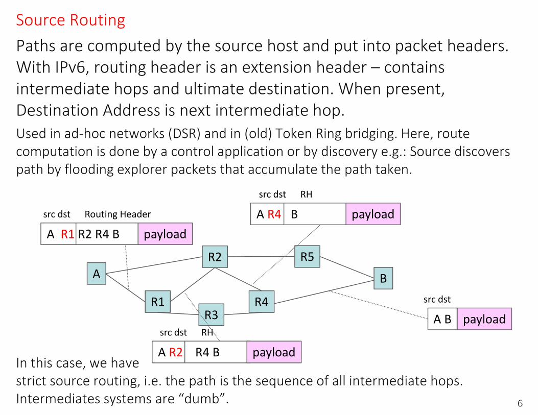
Source RoutingPaths are computed by the source host and put into packet headers. With IPv6, routing header is an extension header – contains intermediate hops and ultimate destination. When present, Destination Address is next intermediate hop. Used in ad‐hoc networks (DSR) and in (old) Token Ring bridging. Here, routecomputation is done by a control application or by discovery e.g.: Source discovers path by flooding explorer packets that accumulate the path taken.
In this case, we have strict source routing, i.e. the path is the sequence of all intermediate hops. Intermediates systems are “dumb”. 6
R1R3
R2
R4
R5A B
A R1 R2 R4 B src dst Routing Header
payloadA R4 B src dst RH
payload
A Bsrc dst
payload
A R2 R4 B src dst RH
payload
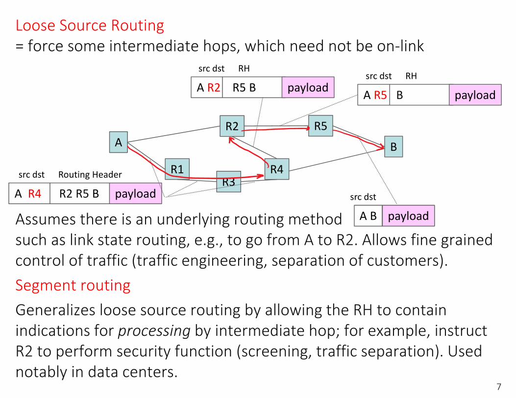
Loose Source Routing= force some intermediate hops, which need not be on‐link
Assumes there is an underlying routing methodsuch as link state routing, e.g., to go from A to R2. Allows fine grained control of traffic (traffic engineering, separation of customers).Segment routingGeneralizes loose source routing by allowing the RH to contain indications for processing by intermediate hop; for example, instruct R2 to perform security function (screening, traffic separation). Used notably in data centers.
7
R1R3
R2
R4
R5A B
A R4 R2 R5 B src dst Routing Header
payload
A R5 B src dst RH
payload
A Bsrc dst
payload
A R2 R5 B src dst RH
payload

2. OSPF with a Single AreaOSPF (Open Shortest Path First) is a very widespread link state routing protocol. We first study it in its simplest form (single area).
Every router hasan interface database (describing its physical connections, learnt by configuration)an adjacency database (describing the neighbour states, learntby the hello protocol)a link state database (the network map, learnt by flooding)
Hello protocol is used to discover neighbouring routers – and to detect failures.When two routers become new neighbours they first synchronize their link state databases. Typically, one router is new and copies what the other already knows.
8

Link State Database and LSAs
Once synchronized, a router sends and accepts link state advertisements (LSAs)
Every router sends one LSA describing its attached networks and neighbouring routersLSAs are flooded to the entire area and stored by all routers in their link state databaseLSAs contains a sequence number and age; only messages with new sequence number are accepted and re‐flooded to all neighbours. Sequence number prevents loops. Age field is used to periodically resend LSA (eg every 30 mn) and to flush invalid LSAs.
9

A Toy Example
10
n1
A
B
n6
D E
n4
n3
C
n5n2
n7
showing interface databases
Net Type cost
n3 Eth stub
n2 p2p 100
n4 p2p 100
At B
Net Type cost
n1 Eth 10
n2 p2p 100
At ANet Type cost
n1 Eth 10
n4 p2p 100
At C
Net Type cost
n6 p2p 10
n5 p2p 20
At DNet Type cost
n6 p2p 10
n7 p2p 100
At E

Routers flood their LSAs throughout area
11
n1
A
B
n6
D E
n4
n3
C
n5n2
n7
router LSA originated by Bn3, Eth, stub;n2, p2p, 100, to A; n4, p2p, 100, to C;
1
2
4
3
5

1, 2 B sends the LSA shown on the picture to A and Cthe LSA describes all the networks attached to B and their costs, as well as the adjacent routers“stub” network means non transit, ie there is no other router on this networka stub network can be reached by only one router; all you need to know is how to reach this router so there is no need to allocate a cost to a stub network
3 C repeats the LSA (unmodified) to D4 C also repeats the LSA to n1. Since n1 is Ethernet, the LSA is
multicast to all OSPF routers on n1. A receives the LSA but does not repeat the LSA on n1 because it received it on n1 from C
5 D repeats LSA to E
12

After FloodingAfter convergence, all routers have received all
LSAs and store them in database.All have the same database.
13
n1
A
B
n6
D E
n4
n3
C
n5n2
n7
router LSA from Bn3, Eth, stub;n2, p2p, 100, to A; n4, p2p, 100, to C router LSA from An2, p2p, 100, to B;n1, eth, 10, DR=Crouter LSA from Cn4, p2p, 100, to B;n5, p2p, 20, to D;n1, eth, 10, DR=Crouter LSA from Dn5, p2p, 20, to C;n6, p2p, 10, to E;router LSA from En6, p2p, 10, to D;n7, eth, stubnetwork LSA from Cn1, eth, 0, A, C
Link State Database at all routers

Ethernet LANs are treated in a special way. In order to avoid that every router on n1, for example, speaks to every other router on n1, the routers elect one designated router per LAN (and one backup designated router). Assume here the designated router is C. Every router that is connected to an Ethernet LAN floods a “router LSA” indicating its connection to this LAN. The designated router “speaks for the switch” and sends a “network LSA” which gives the list of all routers connected to the LAN.
There are (at the time of writing) 11 types of LSAs. In addition to router and network LSAs, the other types are used in the multi‐area case (later section) and with external routes (see BGP module). There are also other LSA types, called “opaque” that are used for purposes other than shortest path routing: opaque LSAs are not used by Dijkstra’s algorithm. They can be used by OSPF extensions that make use of the link‐state database for other purposes (e.g. type 10 LSAs carry information about reservable bandwidth, to be used by QoSrouting). 14

Toy example (cont’d): Router F bootsF discovers neighbours with the hello protocol; assume F discovers C first (C is designated router for n1): F and C establish adjacency (going through a sequence of 8 states, Down to Full). During this process, F and C synchronize their Link State Data Bases (i.e. F copies its LSDB from C). When the state is Full,synchronization is complete and F can now flood a router LSA saying that it is attached to n1; C (as designated router) sends a network LSA to say that F is now on n1.
Then a similar process occurs between F and E, but now the synchronization is very fast since F already has a synchronized link‐state database
15
n1
A
B
n6
D E
n4
n3
C
n5n2 n7
F
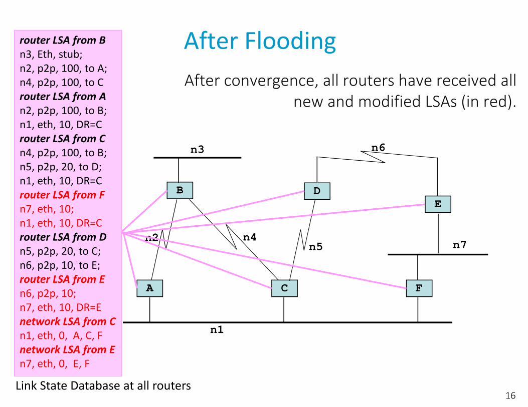
After FloodingAfter convergence, all routers have received all
new and modified LSAs (in red).
16
n1
A
B
n6
D E
n4
n3
C
n5n2
F
n7
router LSA from Bn3, Eth, stub;n2, p2p, 100, to A; n4, p2p, 100, to C router LSA from An2, p2p, 100, to B;n1, eth, 10, DR=Crouter LSA from Cn4, p2p, 100, to B;n5, p2p, 20, to D;n1, eth, 10, DR=Crouter LSA from Fn7, eth, 10;n1, eth, 10, DR=Crouter LSA from Dn5, p2p, 20, to C;n6, p2p, 10, to E;router LSA from En6, p2p, 10;n7, eth, 10, DR=Enetwork LSA from Cn1, eth, 0, A, C, Fnetwork LSA from En7, eth, 0, E, F
Link State Database at all routers
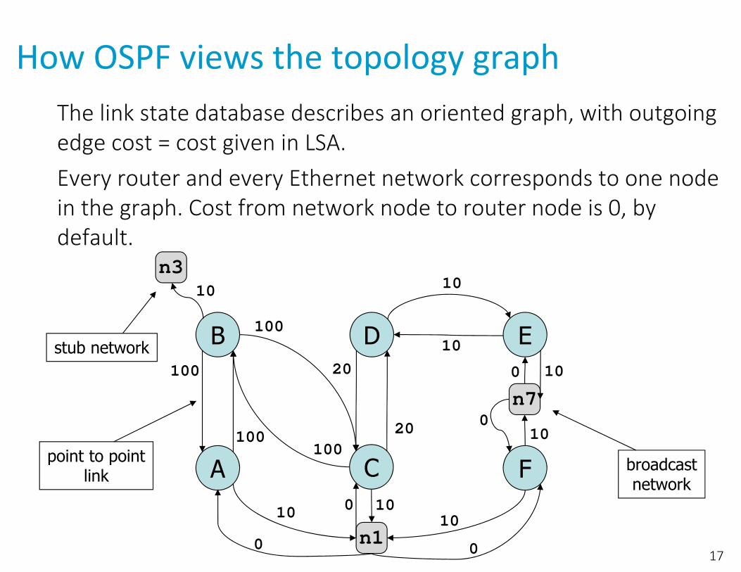
How OSPF views the topology graphThe link state database describes an oriented graph, with outgoing edge cost = cost given in LSA.Every router and every Ethernet network corresponds to one node in the graph. Cost from network node to router node is 0, by default.
17
A
B
C
D
F
E
100
10 10
10
10
10020
n1
100
n7
n3
100
10
20 100
0
0 0
0
stub network
point to pointlink broadcast
network
10
10

Practical Aspects
OSPF packet are sent directly over IP (OSPF=protocol 89 (0x59)). Reliable transmission is managed by OSPF with OSPF Acks and timers.
OSPFv2 supports IPv4 onlyOSPFv3 supports IPv6 and dual‐stack networks
OSPF routers are identified by a 32 bit numberOSPF areas are identified by a 32 bit number
18
3. Path Computation Uses Dijkstra’s Algorithm
Performed at every router, based on link state databaseRouter computes one or several shortest paths to every destination from self
OSPF uses Dijkstra’s shortest paththe best known algorithm for centralized operation
Paths are computed independently at every nodelink state database is same at all routers, but every router performs a different computation as it computes paths from selfsynchronization of databases guarantees absence of persistent loops
19

Dijkstra’s Shortest Path Algorithm
The nodes are 0… ; the algorithmcomputes shortestpaths from node 0.( , ): cost of link ( , ). : set of nodes visited so far.
( ): estimated set of predecessors of node along a shortest path (multiple shortest paths are possible).( ): estimated distance from node 0 to node .
At completion, is the true distance from to .20
𝑚 0 0; 𝑚 𝑖 ∞ ∀ 𝑖 0; 𝑉 ∅ ; 𝑝𝑟𝑒𝑑 𝑖 ∅ ∀𝑖;for 𝑘 0: 𝑁 do
find 𝑖 ∈ 𝑉 that minimizes 𝑚 𝑖if 𝑚 𝑖 is finite
add 𝑖 to 𝑉for all neighbours 𝑗 ∈ 𝑉 of 𝑖
if 𝑚 𝑖 𝑐 𝑖, 𝑗 𝑚 𝑗𝑚 𝑗 𝑚 𝑖 𝑐 𝑖, 𝑗𝑝𝑟𝑒𝑑 𝑗 𝑖
else if 𝑚 𝑖 𝑐 𝑖, 𝑗 𝑚 𝑗𝑚 𝑗 𝑚 𝑖 𝑐 𝑖, 𝑗𝑝𝑟𝑒𝑑 𝑗 𝑝𝑟𝑒𝑑 𝑗 ∪ 𝑖
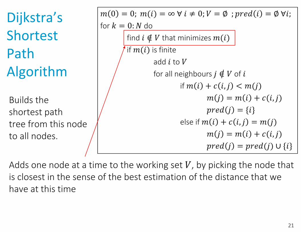
Dijkstra’s Shortest Path Algorithm
Builds theshortest pathtree from this nodeto all nodes.
Adds one node at a time to the working set , by picking the node that is closest in the sense of the best estimation of the distance that we have at this time
21
𝑚 0 0; 𝑚 𝑖 ∞ ∀ 𝑖 0; 𝑉 ∅ ; 𝑝𝑟𝑒𝑑 𝑖 ∅ ∀𝑖;for 𝑘 0: 𝑁 do
find 𝑖 ∈ 𝑉 that minimizes 𝑚 𝑖if 𝑚 𝑖 is finite
add 𝑖 to 𝑉for all neighbours 𝑗 ∈ 𝑉 of 𝑖
if 𝑚 𝑖 𝑐 𝑖, 𝑗 𝑚 𝑗𝑚 𝑗 𝑚 𝑖 𝑐 𝑖, 𝑗𝑝𝑟𝑒𝑑 𝑗 𝑖
else if 𝑚 𝑖 𝑐 𝑖, 𝑗 𝑚 𝑗𝑚 𝑗 𝑚 𝑖 𝑐 𝑖, 𝑗𝑝𝑟𝑒𝑑 𝑗 𝑝𝑟𝑒𝑑 𝑗 ∪ 𝑖

There are multiple versions of Dijkstra’s algorithm. The presented version finds all shortest paths, other versions find only one shortest path to every destination. The version presented is very close to what is really implemented in OSPF (with a difference, next‐hop versus pred(), see later).
The worst‐case complexity of this version is 𝑂 𝑁 where 𝑁 is the number of nodes. More efficient versions of the algorithm have a smaller complexity, 𝑂 𝑁 log 𝑁 𝐸where 𝐸 is the number of links.
The algorithm adds nodes to the visited set by increasing distances from node 0. It is greedy in the sense that at every step it adds one node to the set of visited nodes; the state of this node (distance from node 0 and set of predecessors) is the final value and will not change in later steps of the algorithm.
The last 3 lines are for handling equal cost shortest paths. If one is interested in finding only one shortest path per destination, these 3 lines are deleted.
22

Example: Dijkstra at AInitially
23
A
B
C
D
F
E
100
10
10
10
10
10
100 20
init: V =
m(A)=0m(i)=
pred(i)=
0 ∞
∞ ∞ ∞
∞
m(A)
m(C)

Example: Dijkstra at AAfter step 1
24
A
B
C
D
F
E
100
10
10
10
10
10
100 20
step 1:i=AV={A}m(B)=100pred(B)={A}m(C)=10pred(C)={A}m(F)=10pred(F)={A}
0 10
100 ∞ ∞
10
red arrow from A to B means pred(B)=AB
A

Example: Dijkstra at AAfter step 2
25
A
B
C
D
F
E
100
10
10
10
10
10
100 20
step 2:i=CV={A,C}B, F unchangedm(D)=30pred(D)={C}
0 10
100 30 ∞
10
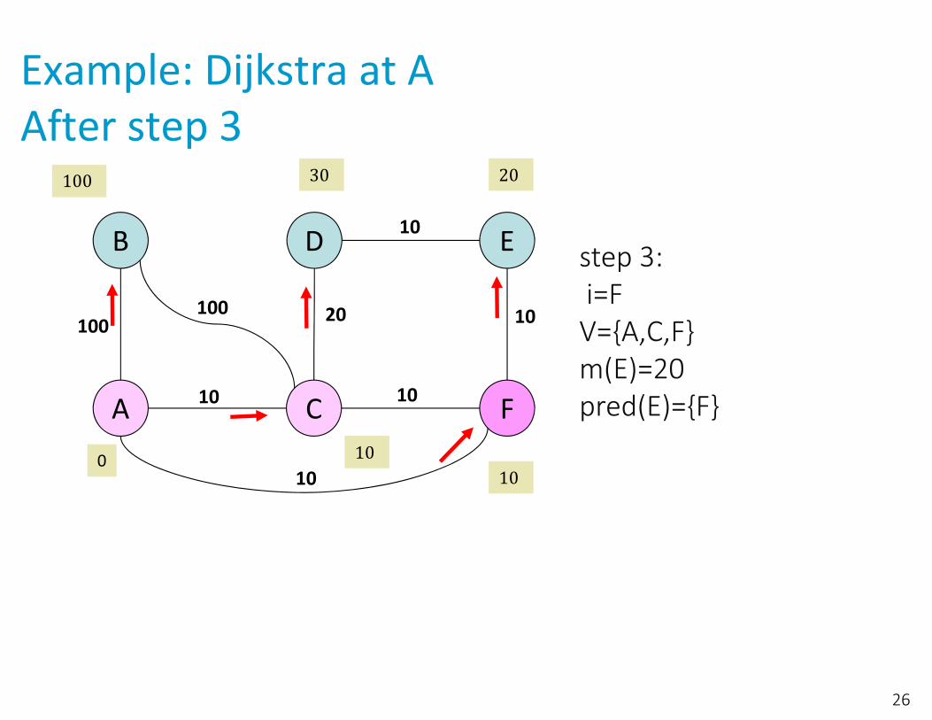
Example: Dijkstra at AAfter step 3
26
A
B
C
D
F
E
100
10
10
10
10
10
100 20
step 3:i=FV={A,C,F}m(E)=20pred(E)={F}
0 10
100 30 20
10

At next step, which node will be added to the working set ?
A. BB. DC. ED. I don’t know
27
A
B
C
D
F
E
100
10
10
10
10
10
100 20
0 10
100 30 20
10
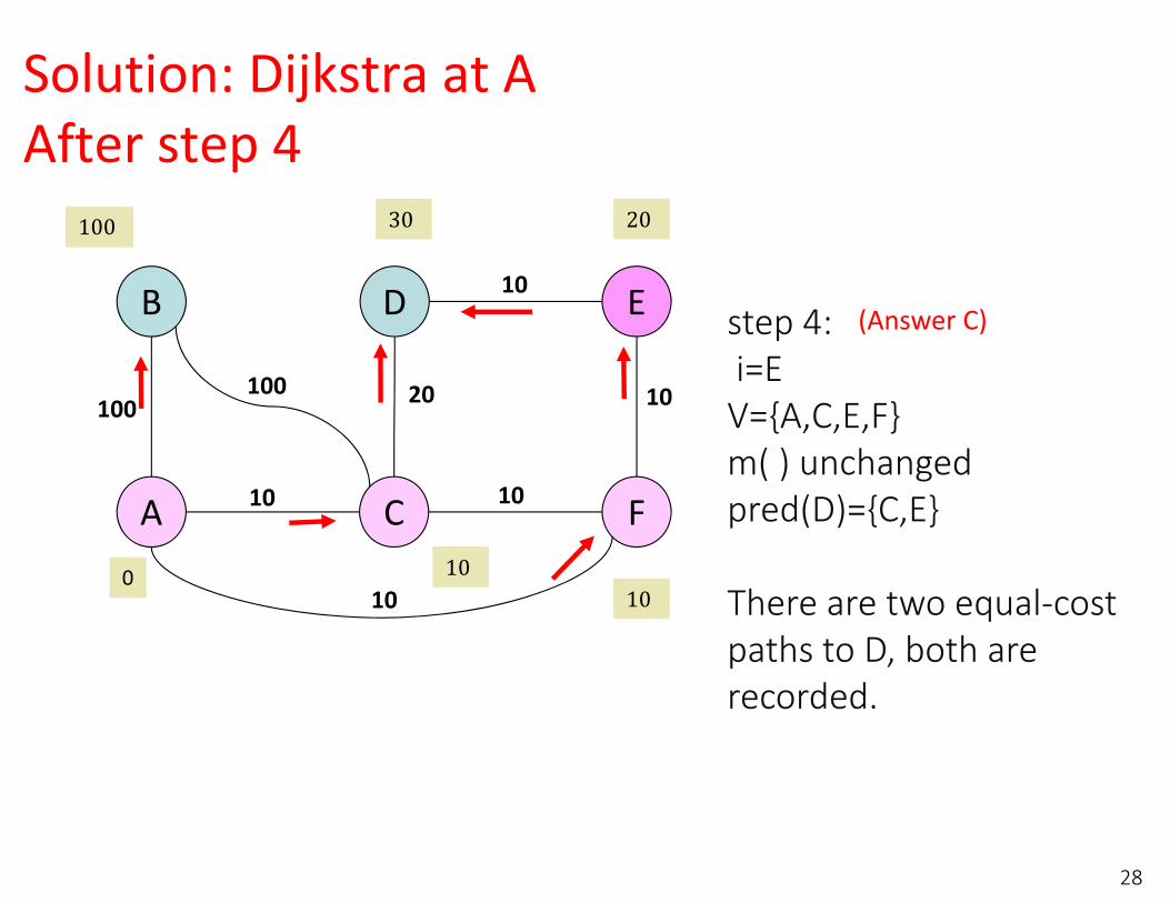
Solution: Dijkstra at AAfter step 4
28
A
B
C
D
F
E
100
10
10
10
10
10
100 20
step 4:i=EV={A,C,E,F}m( ) unchangedpred(D)={C,E}
There are two equal‐costpaths to D, both are recorded.
0 10
100 30 20
10
(Answer C)

Example: Dijkstra at AAfter step 5
29
A
B
C
D
F
E
100
10
10
10
10
10
100 20
step 5:i=DV={A,C,D,E,F}
0 10
100 30 20
10

Example: Dijkstra at AAfter step 6
30
A
B
C
D
F
E
100
10
10
10
10
10
100 20
step 6:i=BV={A,B,C,D,E,F}
this is the final state
0 10
100 30 20
10
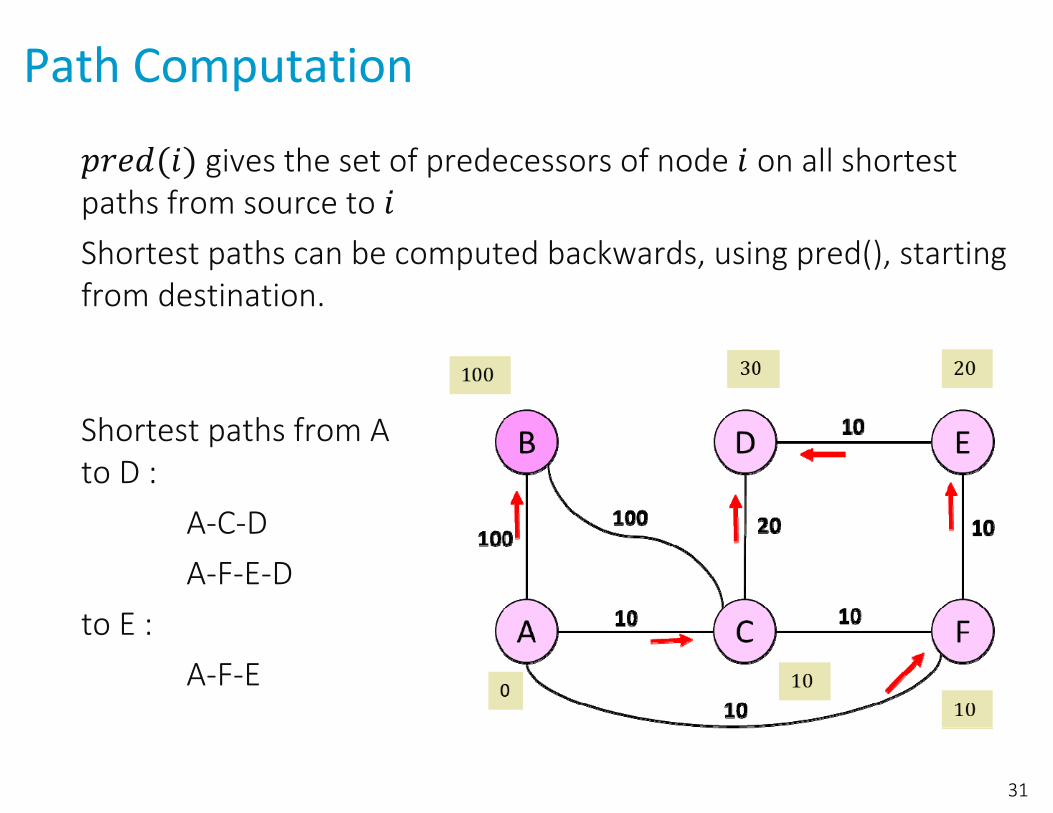
Path Computation
gives the set of predecessors of node on all shortest paths from source to Shortest paths can be computed backwards, using pred(), starting from destination.
Shortest paths from A to D :
A‐C‐DA‐F‐E‐D
to E :A‐F‐E
31

Routing Table
Router A keeps in its routing table the next‐hop and the distance to every destination (not the entire path):
32
Dest Next‐hop
cost
B B 100
C C 10
D C or F 30
E F 20
F F 10
At A

The version of Dijkstra used in OSPF differs from is presented above in that pred() is not used. Instead, the next hop is directly computed during the main loop of the algorithm. This is faster than computing the paths separately, but makes the algorithm more difficult to understand:𝑚 0 0; 𝑚 𝑖 ∞ ∀ 𝑖 0; 𝑉 ∅ ; 𝑛𝑒𝑥𝑡𝐻𝑜𝑝𝑇𝑜 𝑖 ∅ ∀𝑖;for 𝑘 0: 𝑁 do
find 𝑖 ∈ 𝑉 that minimizes 𝑚 𝑖if 𝑚 𝑖 is finite
add 𝑖 to 𝑉for all neighbours 𝑗 ∈ 𝑉 of 𝑖
if 𝑚 𝑖 𝑐 𝑖, 𝑗 𝑚 𝑗𝑚 𝑗 𝑚 𝑖 𝑐 𝑖, 𝑗derive 𝑛𝑒𝑥𝑡𝐻𝑜𝑝𝑇𝑜 𝑗 from 𝑖
else if 𝑚 𝑖 𝑐 𝑖, 𝑗 𝑚 𝑗𝑚 𝑗 𝑚 𝑖 𝑐 𝑖, 𝑗augment 𝑛𝑒𝑥𝑡𝐻𝑜𝑝𝑇𝑜 𝑗 from 𝑖
derive 𝑛𝑒𝑥𝑡𝐻𝑜𝑝𝑇𝑜 𝑗 from 𝑖:if 𝑖 0
𝑛𝑒𝑥𝑡𝐻𝑜𝑝𝑇𝑜 𝑗 𝑗 // 𝑗 is directly connected to 0else
𝑛𝑒𝑥𝑡𝐻𝑜𝑝𝑇𝑜 𝑗 𝑛𝑒𝑥𝑡𝐻𝑜𝑝𝑇𝑜 𝑖 // shortest path to 𝑗 is via 𝑖augment 𝑛𝑒𝑥𝑡𝐻𝑜𝑝𝑇𝑜 𝑗 from 𝑖:
if 𝑖 0𝑛𝑒𝑥𝑡𝐻𝑜𝑝𝑇𝑜 𝑗 𝑗 // 𝑗 is directly connected to 0
else 𝑛𝑒𝑥𝑡𝐻𝑜𝑝𝑇𝑜 𝑗 𝑛𝑒𝑥𝑡𝐻𝑜𝑝𝑇𝑜 𝑗 ∪ 𝑛𝑒𝑥𝑡𝐻𝑜𝑝𝑇𝑜 𝑖 // add shortest path to 𝑗 via 𝑖
33

OSPF Shortest Path Computation
The previous slides showed a very simple graph. In practice, OSPF adds to the graphs nodes to networks, which makes the graph bigger.
To optimize the computation, stub network are removed before applying Dijkstra. Then Dijkstra is run and the routing table contains distances and next hop to routers such as B. Then stub networks such as n3 are added to the routing table one by one, using the information on how to reach the routers such as B that lead to the stub networks.
34
in link state database of every router
Dest Next‐hop cost
B On‐link 100
C On‐link 10
n1 On‐link 10
D F 30
D C 30
n7 F 30
E F 20
F On‐link 10
n3 B 110
Routing table at A
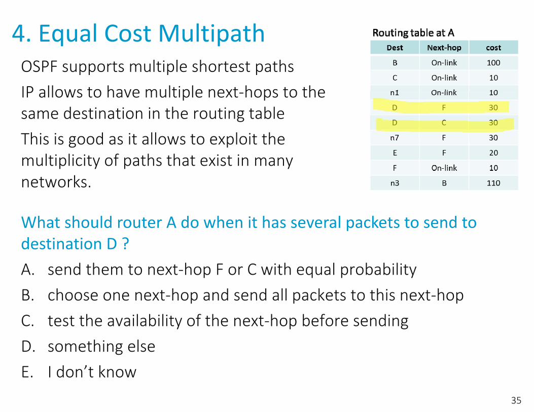
4. Equal Cost MultipathOSPF supports multiple shortest pathsIP allows to have multiple next‐hops to the same destination in the routing tableThis is good as it allows to exploit the multiplicity of paths that exist in many networks.
35
What should router A do when it has several packets to send to destination D ?A. send them to next‐hop F or C with equal probabilityB. choose one next‐hop and send all packets to this next‐hopC. test the availability of the next‐hop before sendingD. something elseE. I don’t know
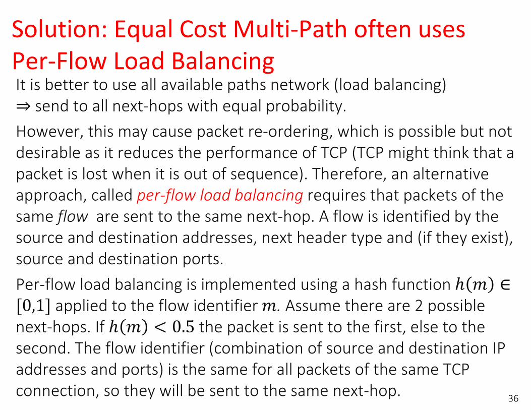
Solution: Equal Cost Multi‐Path often uses Per‐Flow Load BalancingIt is better to use all available paths network (load balancing)
send to all next‐hops with equal probability. However, this may cause packet re‐ordering, which is possible but not desirable as it reduces the performance of TCP (TCP might think that a packet is lost when it is out of sequence). Therefore, an alternative approach, called per‐flow load balancing requires that packets of the same flow are sent to the same next‐hop. A flow is identified by the source and destination addresses, next header type and (if they exist), source and destination ports. Per‐flow load balancing is implemented using a hash function
applied to the flow identifier . Assume there are 2 possible next‐hops. If the packet is sent to the first, else to the second. The flow identifier (combination of source and destination IP addresses and ports) is the same for all packets of the same TCP connection, so they will be sent to the same next‐hop. 36

5. Changes to Topology
Changes to topology occur e.g. when routers or links crash or are rebooted. link or router failures are detected by OSPF’s hello protocol (after several seconds, in general) or by the BFD protocol at a lower layer (fast: after 10 ms ‐ Bidirectional Forwarding Detection, a hello protocol independent of OSPF).
When a router sees a change in the state of a links or a neighbouring router, it sends a new LSA to all its neighbours. All routers update their link state database and propagate the change to the entire OSPF area.
Changes to link state database trigger re‐computation of shortest‐paths and routing tables.
37
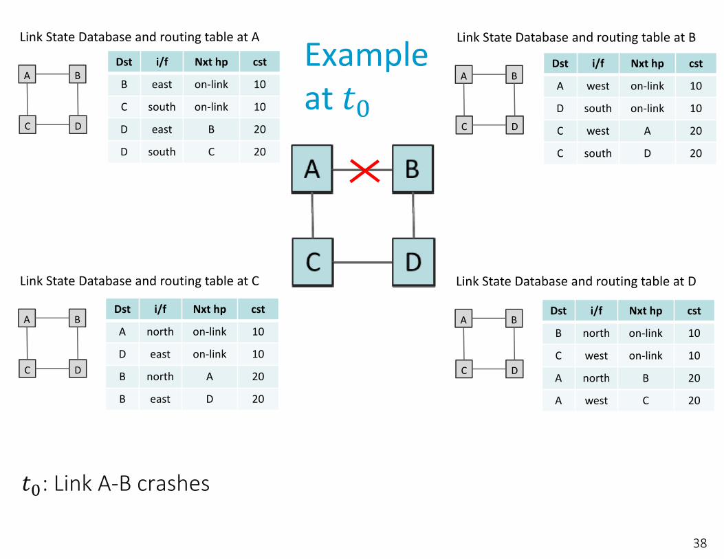
Exampleat
: Link A‐B crashes
38
Dst i/f Nxt hp cst
B east on‐link 10
C south on‐link 10
D east B 20
D south C 20
Link State Database and routing table at A
A B
C D
Link State Database and routing table at C
A B
C D
Link State Database and routing table at B
A B
C D
Link State Database and routing table at D
A B
C D
Dst i/f Nxt hp cst
A north on‐link 10
D east on‐link 10
B north A 20
B east D 20
Dst i/f Nxt hp cst
A west on‐link 10
D south on‐link 10
C west A 20
C south D 20
Dst i/f Nxt hp cst
B north on‐link 10
C west on‐link 10
A north B 20
A west C 20

Exampleat
𝑡 : A detects failure first; declares B as invalid neighbour, declares link A‐B as invalid, updates its link state database, sends a new LSA to C, with origin A and recomputes routing table. A routing loop exists between A and C. Traffic sent by B to A dies on the link. Half of the traffic from D to A is lost.
39
Dst i/f Nxt hp cst
B south C 30
C south on‐link 10
D east B 20
D south C 20
Link State Database and routing table at A
A B
C D
Link State Database and routing table at C
A B
C D
Link State Database and routing table at B
A B
C D
Link State Database and routing table at D
A B
C D
Dst i/f Nxt hp cst
A north on‐link 10
D east on‐link 10
B north A 20
B east D 20
Dst i/f Nxt hp cst
A west on‐link 10
D south on‐link 10
C west A 20
C south D 20
LSA from AA to C, cost=10
Dst i/f Nxt hp cst
B north on‐link 10
C west on‐link 10
A north B 20
A west C 20

Exampleat
𝑡 : C receives LSA from A, updates its link state database, forwards this LSA to D and recomputes routing table. There is no routing loop but traffic sent by B to A dies on the link and half of the traffic from D to A is lost.
40
Dst i/f Nxt hp cst
B south C 30
C south on‐link 10
D east B 20
D south C 20
Link State Database and routing table at A
A B
C D
Link State Database and routing table at C
Link State Database and routing table at B
A B
C D
Link State Database and routing table at D
A B
C D
Dst i/f Nxt hp cst
A north on‐link 10
D east on‐link 10
B north A 20
B east D 20
Dst i/f Nxt hp cst
A west on‐link 10
D south on‐link 10
C west A 20
C south D 20
A B
C D
LSA from AA to C, cost=10
Dst i/f Nxt hp cst
B north on‐link 10
C west on‐link 10
A north B 20
A west C 20

Exampleat
𝑡 : D receives LSA from C, updates its link state database, forwards this LSA to B and recomputes routing table. At about the same time, B now also detects failure; declares A as invalid neighbour, declares link A‐B as invalid, updates its link state database, sends a new LSA to D, with origin B and recomputes routing table. All link state databases now have the same contents and new routes are in place.
41
Dst i/f Nxt hp cst
B south C 30
C south on‐link 10
D east B 20
D south C 20
Link State Database and routing table at A
A B
C D
Link State Database and routing table at C
Link State Database and routing table at B
A B
C D
Link State Database and routing table at D
A B
C D
Dst i/f Nxt hp cst
A north on‐link 10
D east on‐link 10
B north A 20
B east D 20
Dst i/f Nxt hp cst
A south D 30
D south on‐link 10
C west A 20
C south D 20
A B
C D
LSA from BB to D, cost=10
LSA from AA to C, cost=10
Dst i/f Nxt hp cst
B north on‐link 10
C west on‐link 10
A north B 20
A west C 20
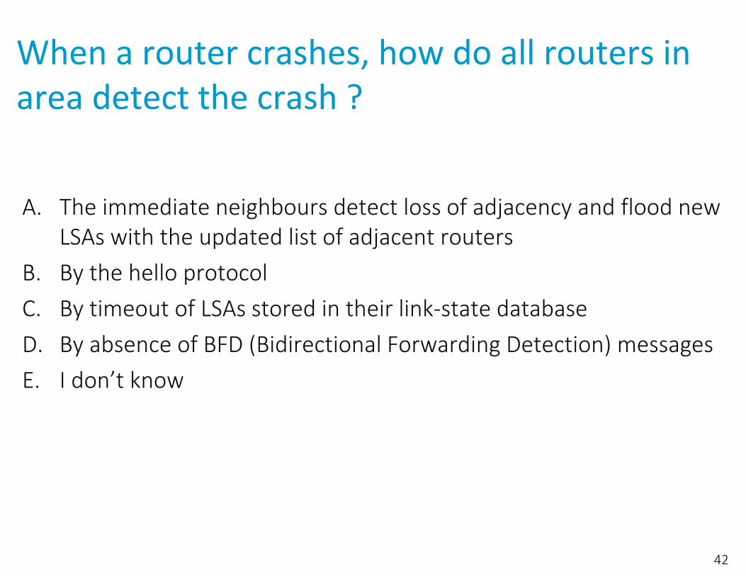
When a router crashes, how do all routers in area detect the crash ?
A. The immediate neighbours detect loss of adjacency and flood new LSAs with the updated list of adjacent routers
B. By the hello protocolC. By timeout of LSAs stored in their link‐state databaseD. By absence of BFD (Bidirectional Forwarding Detection) messagesE. I don’t know
42
Solution
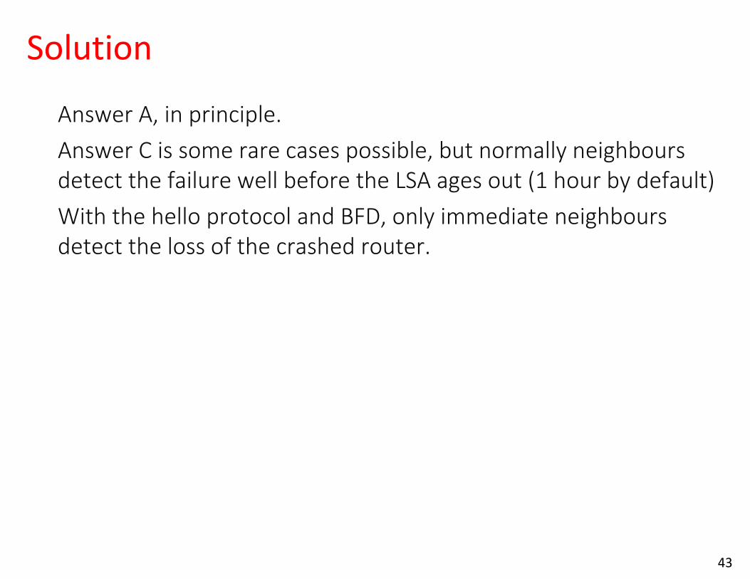
Answer A, in principle.Answer C is some rare cases possible, but normally neighbours detect the failure well before the LSA ages out (1 hour by default) With the hello protocol and BFD, only immediate neighbours detect the loss of the crashed router.
43

6. Security of OSPF
Attacks against routing protocols1. send invalid routing information ⇒ disrupt network operation2. send forged routing information ⇒ change network paths3. denial of service attacks
OSPF security protects against 1. and 2. using authenticationOSPFv2 levels of authentication
type 0: nonetype 1: password sent in cleartext in all packets
type 2: authentication using MD5 (obsolete) or HMAC‐SHAtype 3: similar to type 2 with some improvements (RFC 7474)
OSPFv3 uses IPSEC authenticationsimilar to type 2 and 3 but at IP layer
44

OSPF Type 3 Authentication uses secret, shared keys
Digest and Crypto Sequence Number are appended after OSPF message and sent in IP packet in cleartext.Keys are shared, all routers on same link must have same pre‐installed keys. Keys are expected to have a short lifetime. OSPF does not say how to install the keys, must be done out of band. A key index in authentication header in OSPF message says which key to use.Crypto Sequence Number contains a permanent “boot count” saved on disk to avoid collision of numbers and is large enough to never wrap around (in 10 years). Avoids replay attacks. 45
OSPF message(e.g. hello, update, ack)
IP source addressSecret key (samefor all OSPF routers
on same link)
Cryptographic Hash Algo (e.g. SHA 256)
digest (e.g. 256 bits)
Crypto Sequence Number
7. OSPF with Multiple Areas
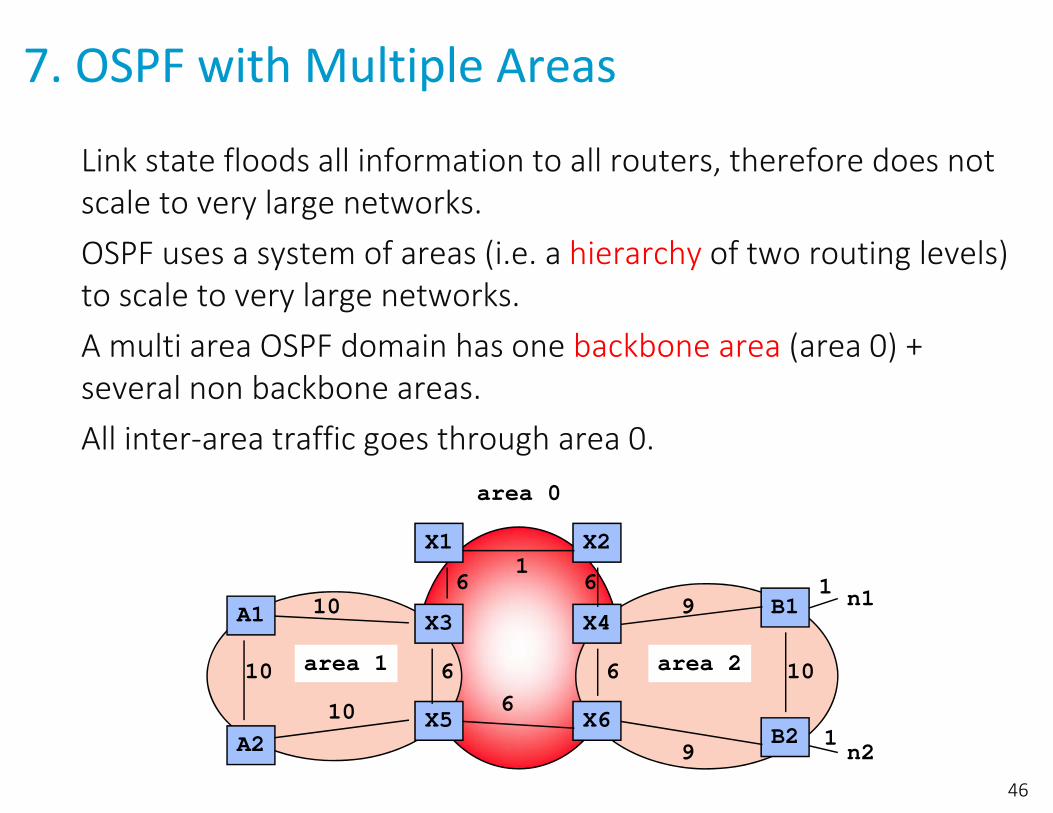
Link state floods all information to all routers, therefore does not scale to very large networks.OSPF uses a system of areas (i.e. a hierarchy of two routing levels) to scale to very large networks. A multi area OSPF domain has one backbone area (area 0) + several non backbone areas.All inter‐area traffic goes through area 0.
46
area 0
B1X4
X1
X3A1
area 2area 1
X2
X6X5B2A2
n1
n2
10
9
9
66
61
6
6
10
10
10
1
1
Principles of OSPF Multi‐Area Operation
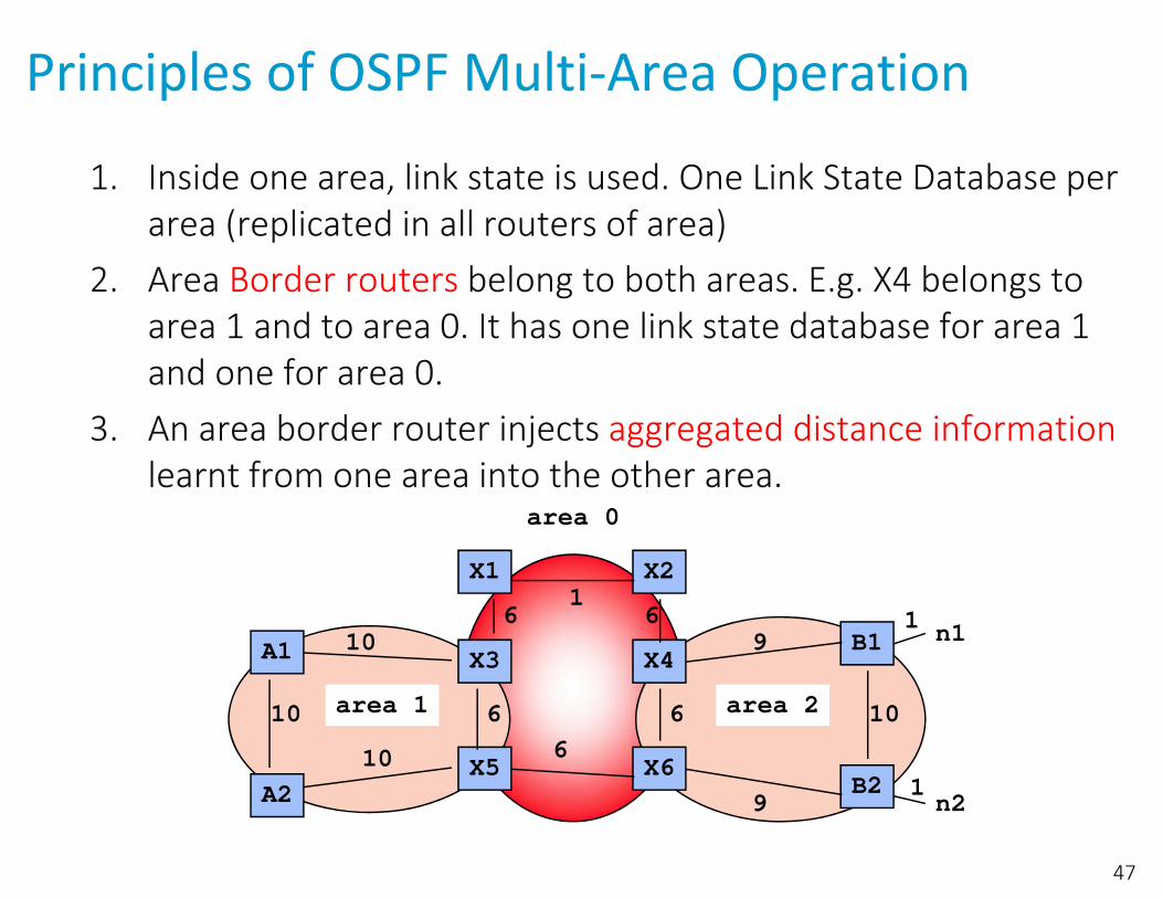
1. Inside one area, link state is used. One Link State Database per area (replicated in all routers of area)
2. Area Border routers belong to both areas. E.g. X4 belongs to area 1 and to area 0. It has one link state database for area 1 and one for area 0.
3. An area border router injects aggregated distance information learnt from one area into the other area.
47
area 0
B1X4
X1
X3A1
area 2area 1
X2
X6X5B2A2
n1
n2
10
9
9
66
61
6
6
10
10
10
1
1

Toy ExampleStep1
All routers in area 2 flood the LSAs originated byB1 and B2 and know of n1 and n2, directly attached to B1 (resp. B2). This is the normal link state operation. All routers in area 2 have the same link state database, shown above.All routers in area 2, including X4 and X6 compute their distances to n1 and n2 (using Dijkstra).
X4: distance to n1 =10, to n2 =16X6: distance to n1 =16, to n2 =10
48
area 0
B1X4
X1
X3A1
area 2area 1
X2
X6X5B2A2
n1
n2
10
9
9
66
61
6
6
10
10
10
1
1
n1
n2
area 2 link state database

Toy ExampleStep2
X4 and X6 each flood into area 0a summary LSA indicating theirdistances to n1 and n2. All routers in area 0 now have the same link state database, shown above.All routers in area 0, including X3 and X5 compute their distances to networks outside the area (such as n1) using the Bellman‐Ford formula
∈ where BR is a border router
49
n1
n2
area 0 link state database n1, d=10n2, d=16
n1, d=16n2, d=10
area 0
B1X4
X1
X3A1
area 2area 1
X2
X6X5B2A2
n1
n2
10
9
9
66
61
6
6
10
10
10
1
1
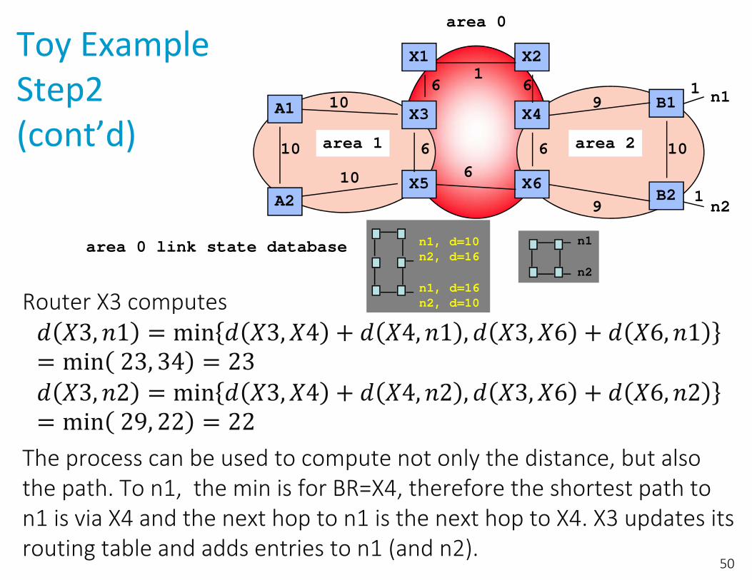
Toy ExampleStep2(cont’d)
Router X3 computes
The process can be used to compute not only the distance, but also the path. To n1, the min is for BR=X4, therefore the shortest path to n1 is via X4 and the next hop to n1 is the next hop to X4. X3 updates its routing table and adds entries to n1 (and n2).
50
n1
n2
area 0 link state database n1, d=10n2, d=16
n1, d=16n2, d=10
area 0
B1X4
X1
X3A1
area 2area 1
X2
X6X5B2A2
n1
n2
10
9
9
66
61
6
6
10
10
10
1
1

Toy ExampleStep 3
X3 and X5 each flood into area 1a summary LSA indicating theirdistances to n1 and n2. All routers in area 1 now have the same link state database, shown above.All routers in area 1 compute their distances to networks outside the area (such as n1) using the Bellman‐Ford formula
∈ where BR is a border router. E.g. A1 finds that the distance to n1 is 33 and the shortest path is via X3.
51
n1
n2
n1, d=10n2, d=16
n1, d=16n2, d=10
n1, d=23n2, d=22
n1, d=22n2, d=16
area 1 link state
database
area 0
B1X4
X1
X3A1
area 2area 1
X2
X6X5B2A2
n1
n2
10
9
9
66
61
6
6
10
10
10
1
1

When applying the Bellman‐Ford formula to compute
, how does a router such as A1 know the values of and
?
from its routingtable and fromits link state database
from its routingtable and fromits link state database
C. both from the routing tableD. both from the link state databaseE. I don’t know
52

Solution
All routers in area 1 have only their routing tables this
information
The border routers are in area 1, so A1 knows d(self, BR)
from its routing table (after applying Dijkstra).
d(BR, n1) is known from an external‐LSA, i.e. is in the link‐state database of A1 (and of
all routers in area 1).Answer A.
53
X3A1
area 1
X5A2
6
10
10
10n1, d=23n2, d=22
n1, d=22n2, d=16

How many link state databases does router X3 have ?
A. 1B. 2C. 3D. 0E. I don’t know
54
area 0
B1X4
X1
X3A1
area 2area 1
X2
X6X5B2A2
n1
n2
10
10
10
66
61
6
6
10
10
10

Solution
Answer B.X3 belongs to area 0 and to area 1. It has onelink‐state databasefor each.
55
area 0
B1X4
X1
X3A1
area 2area 1
X2
X6X5B2A2
n1
n2
10
9
9
66
61
6
6
10
10
10
1
1
n1, d=10n2, d=16
n1, d=16n2, d=10
n1, d=23n2, d=22
n1, d=22n2, d=16
Comments
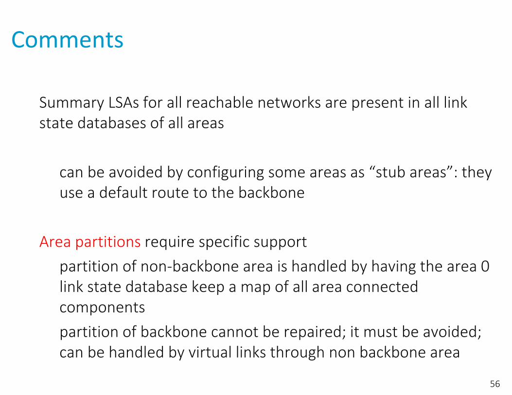
Summary LSAs for all reachable networks are present in all link state databases of all areas
can be avoided by configuring some areas as “stub areas”: they use a default route to the backbone
Area partitions require specific supportpartition of non‐backbone area is handled by having the area 0 link state database keep a map of all area connected componentspartition of backbone cannot be repaired; it must be avoided; can be handled by virtual links through non backbone area
56

8. Other Uses of Link State Routing
Link state routing (OSPF or IS‐IS) provides a complete view of area to every node. This can be used to provide advanced functions:
multi‐class routing: compute different routes for different types of services (e.g. voice, video)
explicit routes (with source routing): an edge router computes the entire path, not just the next‐hop, and writes it in the packet header. Avoids transient loops / supports fast re‐route after failure.
57

Example: LS bridging
Assume you want to bridge VLANs across a campus. One solution: tunnel MAC packets in IP. Problem: automatic creation of tunnels.
Can you imagine a solution using Link State Routing in R1, R2, … ?A. Routers R1, R2 … discover
which VLAN is active on any of their ports and put this information in the link state database
B. Routers R1, R2 … overhear all MAC source addresses and put the information in the link state database
C. Both of these solutions seem bad to meD. I don’t know
58
R1
R2
R3
R4
R6
R7
R5
VLAN2
VLAN2
VLAN2
VLAN1
VLAN1
VLAN1

Solution
B does not help since MAC addresses don’t say in which VLAN the machine isA is a feasible solution: routers can create VLAN tunnels (MAC in IP !) e.g. using IP multicastThis is what Cisco’s TRILL does (with IS‐IS instead of OSPF)
IEEE’s SPB is similar (with MAC in MAC encapsulation); supports explicit routes with 802.1av for video networking in studios.
59
MAC in IP tunnels

What is the maximum value of ?Node A sends a total traffic equal to b/s, half toB, half to C.Same for B and C.Link capacities are 1 Gb/s in every direction(full duplex). OSPF costs are 10.Possible configurations: OSPF Routers or Transparent Bridges/STP
A. With OSPF: Gb/s; with TB Gb/s; B. With OSPF: Gb/s; with TB Gb/s; C. With OSPF: Gb/s; with TB Gb/s; D. With OSPF: Gb/s; with TB Gb/s; E. I don’t know.
60
B
A
C

SolutionOSPF routers use shortest paths. Traffic from anynode uses the direct link (same is true with anydistance vector, which that also computesshortest paths, and with TRILL bridges).From A to B, the traffic flow is , sameon every link and each direction. The constraints are Gb/s thus Gb/s,
With transparent bridges, a spanning tree isbuilt, one of the links is disabled. Total trafficon every link and every direction is , thus Gb/s.
Answer B.
61
shortestpath
spanningtree
B
A
C
B
A
C

9. Software Defined NetworkingIn principle, an IP router uses the destination address and longest prefix match to decide where to send a packet.Some networks want more control; e.g. handle mission critical traffic with high priority; ban non‐HTTP traffic; send suspicious traffic to a machine that does deep packet inspection.
62
From [S. Vissicchio et al., “Central Control Over
Distributed Routing”, ACM Sigcomm 2015]
http://fibbing.net
A sudden traffic surge is noticed from A, D and E to
F (red). The network operator would like to divert all red traffic to
scrubber for inspection. Blue traffic should not be
modified.

Per‐Flow ForwardingThis is why some routers can be configured with per‐flow forwarding rules.When a packet has to be forwarded, such a router does:
Look for a rule match in the list of (priority‐ordered) per‐flow forwarding rules (also called flow table)if one or several matches exist, follow the rule with highest priorityIf no rule matches, go to the IP forwarding table and do longest prefix match
Same can be used in switches (per flow tables then complement the MAC forwarding table)
63
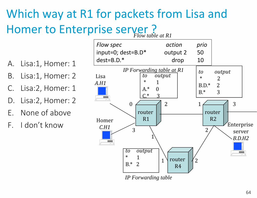
Which way at R1 for packets from Lisa and Homer to Enterprise server ?
A. Lisa:1, Homer: 1B. Lisa:1, Homer: 2C. Lisa:2, Homer: 1D. Lisa:2, Homer: 2E. None of aboveF. I don’t know
64
router R1
router R2
router R4
LisaA.H1
Enterprise serverB.D.H2
2 1
2
21
3
to output* 1A.* 0C.* 3
to output* 2B.D.* 2B.* 3
to output* 1B.* 2
30
IP Forwarding table at R1
IP Forwarding table
HomerC.H1
1
Flow spec action prioinput=0; dest=B.D* output 2 50 dest=B.D.* drop 10
Flow table at R1

Solution
Answer EPackets from Lisa to enterprise server match the two flow rules; the first one has higher priority and is applied. Packets are forwarded to port 2. Since there is a match in flow table, the IP forwarding table is not used.
Packets from Homer to enterprise server match the second flow rule and are dropped by R1.
The combined effect of the flow table and the IP forwarding table at R1 is such that1. all traffic to B.D.* is killed except if arriving on input 02. traffic to B.D.* that is not killed is forwarded to output 23. traffic to B.* and not B.D.* is forwarded to output 1
65
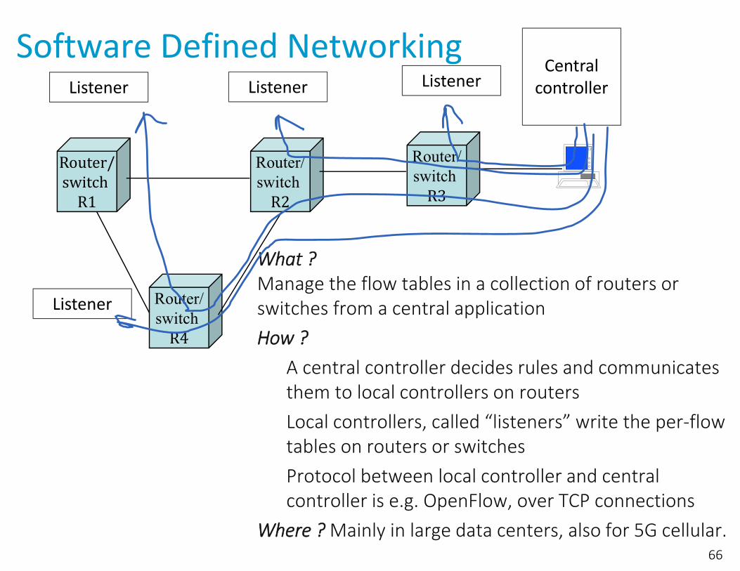
Software Defined Networking
What ?Manage the flow tables in a collection of routers or switches from a central applicationHow ?
A central controller decides rules and communicates them to local controllers on routersLocal controllers, called “listeners” write the per‐flow tables on routers or switchesProtocol between local controller and central controller is e.g. OpenFlow, over TCP connections
Where ?Mainly in large data centers, also for 5G cellular.66
Router/switch
R1
Router/switch
R2
Router/switch
R4
Router/switch
R3
Listener Listener
Listener
ListenerCentral
controller
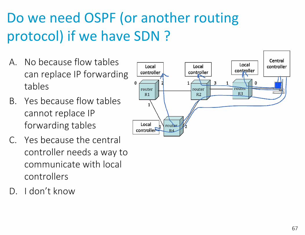
Do we need OSPF (or another routing protocol) if we have SDN ?
A. No because flow tables can replace IP forwarding tables
B. Yes because flow tables cannot replace IP forwarding tables
C. Yes because the central controller needs a way to communicate with local controllers
D. I don’t know
67

Solution
Answer CThe central controller communicates with the local controllers in routers over TCP connections. This needs that IP forwarding tables are functional, which in turn requires OSPF or some other routing protocol.
68
Conclusion
OSPF (and routing protocols) automatically build connectivity and repair failures. With link state routing:• All routers compute their own link state database, replicated in
all routers• All routers compute their routing tables using Dijkstra and the
link state database• Convergence after failure is fast (if detection is fast)• Supports flexible cost definitions; can be used for routing
specific flows in different ways• Large domains must be split into areasMore control can be obtained by an outside application (SDN). SDN is used today primarily with switches, but also starts to be used with routers.
69


![Open Shortest Path First Routing Under Random Early Detectionsd-research.uwaterloo.ca/papers/Networks-OSPF-Routing-with-RED.pdf · First (OSPF) routing protocol [35], where OSPF requires](https://static.documents.pub/doc/80x56/5f746308e2e9e43294254a6e/open-shortest-path-first-routing-under-random-early-detectionsd-first-ospf-routing.jpg)


