Lip Synchronization in Video Conferencing -...

C H A P T E R 7

Lip Synchronization in Video Conferencing

Chapter 3, “Fundamentals of Video Compression,” went into detail about how audio and video streams are encoded and decoded in a video conferencing system. However, the last processing step in the end-to-end chain involves ensuring that the decoded audio and video streams play with perfect synchronization. This chapter focuses on audio and video; however, video conferencing systems can synchronize any type of media to any other type of media, including sequences of still images or 3D animation. Two issues complicate the process of achieving synchronization:

■ Real-time Transport Protocol (RTP)-based video conferencing systems separate audio and video into different RTP streams on the network.

■ Video conferencing systems also typically have separate processing pipelines for audio and video within the sender and receiver endpoints.

This chapter covers the process of realigning those streams at the receiver.

Understanding Lip Sync Skew

Lip sync is the general term for audio/video synchronization, and literally refers to the fact that visual lip movements of a speaker must match the sound of the spoken words. If the video and audio displayed at the receiving endpoint are not in sync, the misalignment between audio and video is referred to as skew. Without a mechanism to ensure lip sync, audio often plays ahead of video, because the latencies involved in processing and sending video frames are greater than the latencies for audio.

Human Perceptions

User-perceived objection to unsynchronized media streams varies with the amount of skew—for instance, a misalignment of audio and video of less than 20 milliseconds (ms) is considered imperceptible. As the skew approaches 50 ms, some viewers will begin to notice the audio/video mismatch but will be unable to determine whether video is leading or lagging audio. As the skew increases, viewers detect that video and audio are out of sync and can also determine whether video is leading or lagging audio. At this point, the video/audio offset distracts users from the

224 Chapter 7: Lip Synchronization in Video Conferencing

video conference. When the skew approaches one second, the video signal provides no benefit—viewers will ignore the video and focus on the audio.

Human sensitivity to skew differs greatly from person to person. For the same audio/video skew, one person might be able to detect that one stream is clearly leading another stream, whereas another person might not be able to detect any skew at all.

A research paper published by the IEEE reveals that most viewers are more sensitive to audio/video misalignment when audio plays before the corresponding video, because hearing the spoken word before seeing the lips move is more “unnatural” to a viewer (Blakowski and Steinmetz 1996).

Sensitivity to skew is also determined by the frame rate and resolution: Viewers are more sensitive to skew when watching higher video resolution or higher frame rate.

Report IS-191 issued by the Advanced Television Systems Committee (ATSC) recommends guidelines for maximum skew tolerances for broadcast systems to achieve acceptable quality. The guidelines model the end-to-end path by assuming that a single encoder at the distribution center receives both audio and video streams, digitizes the streams, assigns time stamps, encodes the streams, and then sends the encoded data over a network to a receiver. The guidelines specify that on the sending side, at the input to the encoder, the audio should not lead the video by more than 15 ms and should not lag the video by more than 45 ms. This possible lead or lag might arise from uncertainty in the latencies through the digitizing/capture hardware and occurs before the encoder assigns time stamps to the digitized media streams.

At the receiving side, the receiver plays the audio and video streams according to time stamps assigned by the encoder. But again, there is an uncertainty in the latency of each stream through the playout hardware. The guidelines stipulate that for each stream, this uncertainty should not exceed ±15 ms; this tolerance is an absolute tolerance that applies to each stream. Based on these guidelines, two requirements emerge for acceptable lip sync tolerance:

■ Criterion for leading audio—In the worst-case-permitted scenario, audio leads video at the input to the encoder by 15 ms. The receiver plays the audio stream too far ahead by 15 ms while playing the video stream too far behind by 15 ms. As a result, the maximum amount by which audio may lead video at the presentation device of the receiver is 15 ms + 15 ms + 15 ms = 45 ms.

Understanding Lip Sync Skew 225

■ Criterion for lagging audio—In the worst-case-permitted scenario, audio lags video at the input to the encoder by 45 ms. The receiver plays the audio stream too far behind by 15 ms while playing the video stream too far ahead by 15 ms. As a result, the maximum amount by which audio may lag video at the presentation device of the receiver is 45 ms + 15 ms + 15 ms = 75 ms.

Measuring Skew

Audio/video skew is measured on the output device at presentation time. The output device is also called the presentation device. The definition of presentation time depends on the output device:

■ For video displays, the presentation time of a frame in a video sequence is the moment that the image flashes on the screen.

■ For audio devices, the presentation time for a sample of audio is the moment that the endpoint speakers emit the audio sample.

The presentation times of the audio and video streams on the output devices must match the capture times at the input devices. These input devices (camera, microphone) are also called capture devices. The method of determining the capture time depends on the media:

■ For a video camera, the capture time for a video frame is the moment that the charge-coupled device (CCD) in the camera captures the image.

■ For a microphone, the capture time for a sample of audio is the moment that the microphone transducer records the sample.

For each type of media, the entire path from capture device on the sender to presentation device on the receiver is called the end-to-end path.

A lip sync mechanism must ensure that the skew at the presentation device on the receiver is as close as possible to zero. In other words, the relationship between audio and video at presentation time, on the presentation device, must match the relationship between audio and video at capture time, on the capture device, even in the presence of numerous delays in the entire end-to-end path, which might differ between video and audio.

NOTE When designing a video conferencing product, you will find it beneficial to find a “skew test person” who is highly sensitive to audio/video misalignment, to provide the worst-case subjective opinion on skew tolerance.


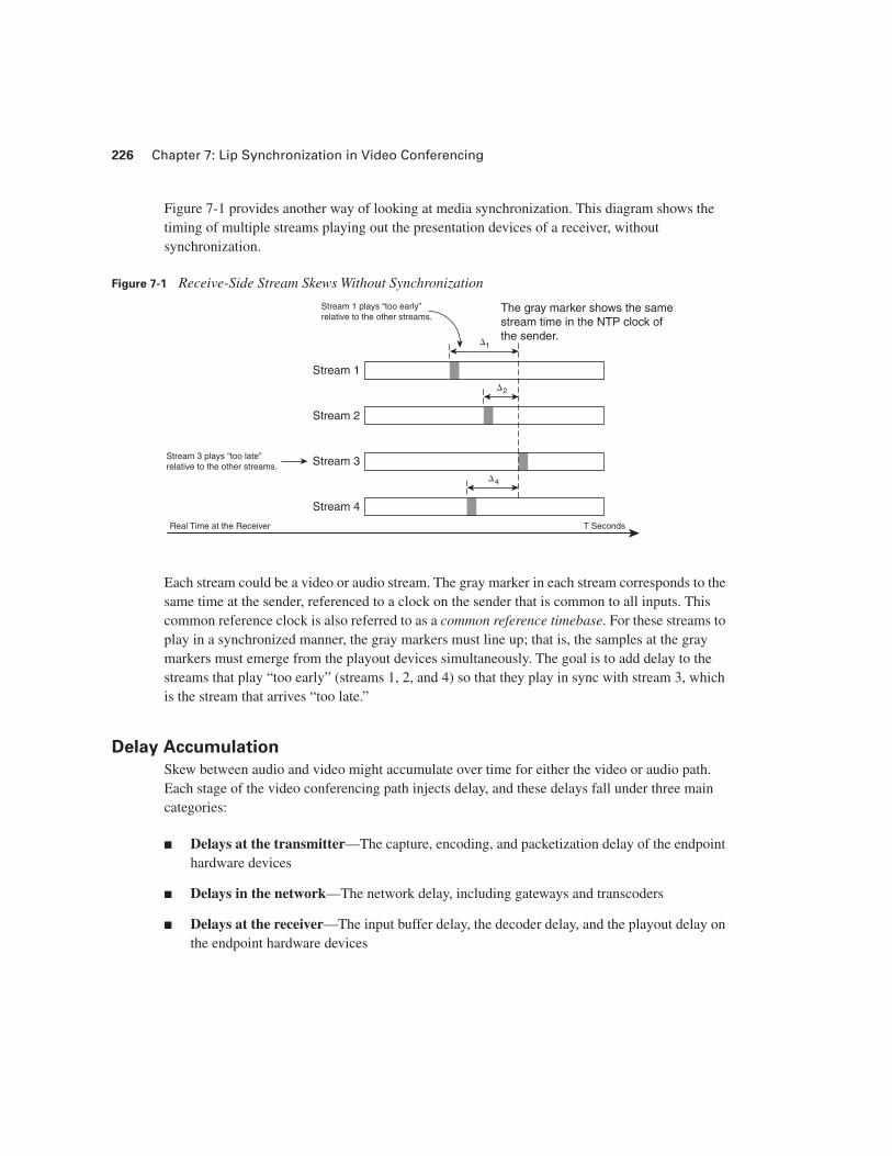
Figure 7-1 provides another way of looking at media synchronization. This diagram shows the timing of multiple streams playing out the presentation devices of a receiver, without synchronization.

Figure 7-1 Receive-Side Stream Skews Without Synchronization

Each stream could be a video or audio stream. The gray marker in each stream corresponds to the same time at the sender, referenced to a clock on the sender that is common to all inputs. This common reference clock is also referred to as a common reference timebase. For these streams to play in a synchronized manner, the gray markers must line up; that is, the samples at the gray markers must emerge from the playout devices simultaneously. The goal is to add delay to the streams that play “too early” (streams 1, 2, and 4) so that they play in sync with stream 3, which is the stream that arrives “too late.”

Delay Accumulation

Skew between audio and video might accumulate over time for either the video or audio path. Each stage of the video conferencing path injects delay, and these delays fall under three main categories:

■ Delays at the transmitter—The capture, encoding, and packetization delay of the endpoint hardware devices

■ Delays in the network—The network delay, including gateways and transcoders

■ Delays at the receiver—The input buffer delay, the decoder delay, and the playout delay on the endpoint hardware devices

Stream 1 plays “too early”relative to the other streams.

Stream 2

Stream 3

Stream 4

Stream 1

The gray marker shows the samestream time in the NTP clock ofthe sender.

Stream 3 plays “too late” relative to the other streams.

Real Time at the Receiver T Seconds

4

2

1

Understanding Lip Sync Skew 227

However, most of these delays are unknown and difficult to measure and change over time. This means that the mechanism for achieving lip sync should not attempt to measure and account for each individual delay in the end-to-end media path. Instead, the mechanism must work in the presence of variable, unknown path delays.

Most video conferencing equipment transmits audio and video over a network using RTP, which multiplexes audio and video into separate network streams. This method is in contrast to the format for DVDs, which multiplex the audio and video streams into a single stream called an MPEG2 program stream. Because the audio and video streams of a video conference remain separated through the network from endpoint to endpoint, each stream might experience different network delays.

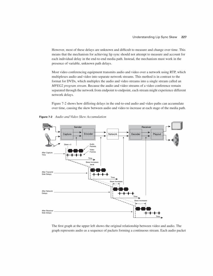
Figure 7-2 shows how differing delays in the end-to-end audio and video paths can accumulate over time, causing the skew between audio and video to increase at each stage of the media path.

Figure 7-2 Audio and Video Skew Accumulation

The first graph at the upper left shows the original relationship between video and audio. The graph represents audio as a sequence of packets forming a continuous stream. Each audio packet

Capture

Sender

Encoder Decoder

Receiver

PlayoutNetwork

Skew = 0

Skew Increases

Skew Increases

Skew Increases

AudioPackets

VideoFrames

Time

Time

Time

Time

After CaptureTime

After ReceiverSide Delays

After NetworkDelays

After TransmitSide Delays


spans a duration of time corresponding to the audio data it contains. In contrast, the graph represents video as a sequence of frames, where each frame exists for a single instant of time. The figure shows a scenario in which the skew between audio and video increases at three stages of the end-to-end path from sender to receiver: after the sender-side delays, after the network delays, and after the receiver-side delays. To understand how delays creep into each stage, it is necessary to look at how each stage processes data, starting with the network path.

Delays in the Network Path

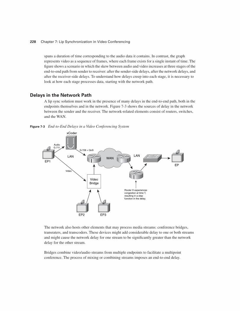
A lip sync solution must work in the presence of many delays in the end-to-end path, both in the endpoints themselves and in the network. Figure 7-3 shows the sources of delay in the network between the sender and the receiver. The network-related elements consist of routers, switches, and the WAN.

Figure 7-3 End-to-End Delays in a Video Conferencing System

The network also hosts other elements that may process media streams: conference bridges, transraters, and transcoders. These devices might add considerable delay to one or both streams and might cause the network delay for one stream to be significantly greater than the network delay for the other stream.

Bridges combine video/audio streams from multiple endpoints to facilitate a multipoint conference. The process of mixing or combining streams imposes an end-to-end delay.

EP

xCoder

LAN LANWAN

EP1

Video

EP2 EP3

VideoBridge

AudioG.711

G.728 + QoS

Router X experiencescongestion at time T,resulting in a stepfunction in the delay.

Lip Sync Approaches 229

Transraters re-encode a video stream into a lower bit rate to send the bitstream through a lower-bandwidth network or to a lower-bandwidth endpoint. Transraters typically apply only to video streams.

Transcoders may exist in the network to change the codec type and may apply to either audio or video streams. Figure 7-3 shows a transcoder that translates from G.711 to G.728. A video conferencing network configuration might require transcoders for two reasons:

■ To reduce the bit rate—Figure 7-3 shows a scenario in which an audio transcoder converts a high-bandwidth audio stream into a low-bandwidth stream. In this case, the high-bandwidth G.711 stream arrives at the transcoder on a high-bandwidth LAN, and the bridge must transcode the audio stream into a lower-bandwidth G.728 version suitable for a low-bandwidth WAN. When a bridge uses a transcoder for the sole purpose of changing the bit rate, it is still called a transcoder, even if the end effect is that of a transrater.

■ To bridge two endpoints with different codec capabilities—One example for audio is the process of converting from an H.320-centric G.729 codec to an H.323-centric G.723 codec. An example for video is the process of converting from an H.323-centric H.263 codec to an H.320-centric H.261 codec.

Delays for audio and video on some segments of the network might differ due to different quality of service (QoS) levels. Figure 7-3 shows a router configured with QoS to provide lower latency for audio than for video. This difference in quality might be continuous or might arise only when the router suffers heavier-than-normal network congestion.

The congestion level of routers might cause the delays for either audio or video to fluctuate over time. In the figure, router X temporarily experiences a heavy load at time T, causing it to momentarily increase the delay of packets through its queue.

In addition to these short-term events, the long-term, steady-state network path taken by either stream might abruptly change as a result of a change in the dynamic IP routing. Any change in IP routing results in new steady-state end-to-end delays.

Lip Sync Approaches

Video conferencing endpoints generally take two approaches to achieve lip sync:

■ Poor Man’s lip sync—This method assumes that delays in the end-to-end media paths are known and constant. It relies on packet arrival times for synchronization.

■ Common Reference lip sync—This method assumes that delays in the end-to-end media paths are not easily known and might vary. It relies on a common reference timebase for both audio and video streams.


Poor Man’s Lip Sync

The simplest incarnation of a lip sync algorithm is known as Poor Man’s lip sync. In this method, the receiver uses one criterion to synchronize audio and video: Packets of audio and video that arrive simultaneously at the network interface of the receiver are considered to be synchronized to each other. This approach is fundamentally flawed because delays in the end-to-end path vary both in space (at different points of the path) and time (fluctuations in delay from one moment to the next). In addition, trying to measure, predict, and compensate for these variable delays in the end-to-end path is a futile effort.

When using Poor Man’s lip sync, the conferencing system must make several assumptions about the sender, receiver, and network infrastructure:

■ Sender—For Poor Man’s lip sync, the sender generally assumes that the network delay to the receiver is the same for both audio and video streams. However, scenarios might arise in which the delays differ. For instance, a transcoder might be present in the audio path but not the video path. Or, the network might assign a higher QoS to one path, resulting in lower delay for that stream.

■ Receiver—When operating with Poor Man’s lip sync, the receiver must derive a relationship between the time stamps of the two streams by observing the relationship between the packet arrival times and timestamps for each individual stream, and then using that information to derive a relationship between the packet timestamps of the two streams. However, the receiver might have difficulty deriving an accurate relationship, because packet arrival times vary because of arrival-time jitter.

■ Network infrastructure—Poor Man’s lip sync makes the following invalid assumptions:

— The average network delay remains constant over the long term.

— The instantaneous network delay remains constant over the short term.

When you are using Poor Man’s lip sync, if the sender cannot compensate for network delays, specialized video conferencing network infrastructure might be necessary between the two endpoints. This infrastructure readjusts the synchronization of audio and video streams by adding delay to one stream or another.

An unfortunate byproduct of Poor Man’s lip sync is that it often results in the sender or the network infrastructure delaying one or more streams to attempt synchronization at the receiver. However, for maximum flexibility, delays should be introduced only at the receivers, which leads to one of the corollaries of robust lip sync:

Only the receiver should delay media streams to achieve lip sync.

Lip Sync Approaches 231

This corollary is necessary for two reasons:

■ If the end-to-end audio delay is already significant, the receiver might prefer to avoid adding more delay to the audio stream and forego lip sync. Instead, the receiver might want to go without audio and video synchronization to maintain the lowest audio end-to-end delay for the best interaction between conference participants. The end user makes this decision via the user interface (UI) of the receiver endpoint. Therefore, other entities on the network should not overrule this decision.

■ The process of delaying one stream to achieve lip sync should be left to the receiver, because the receiver can take into account its own internal delays in each media path at the same time that it delays one stream or the other to synchronize media. For instance, if audio arrives at the receiver ahead of video, normally the receiver must delay the audio stream to achieve lip sync with the video. However, an input buffer in the receiver might already provide some or all of this delay.

The Offset Slider of Doom

A device commonly used as a sidekick to Poor Man’s lip sync is the offset slider of doom. In older PC-based video conferencing and streaming systems, the input devices often had considerable delay in the capture pipeline. In addition, these devices generally did not provide a way of correlating captured samples with real time. To make matters worse, different capture devices had different delays. The sender would make a guess as to the capture pipeline delay for audio and video but would require user input to fine-tune these guesses by means of an offset slider, which consisted of a slider bar in the configuration options of the user interface.

With the slider in the middle of its range, the sender would use its nominal guesses for audio and video pipeline latency. The end user could move the slider to the right, which would increase the guess for the audio capture pipeline delay, while keeping the video pipeline delay the same. Or, the user could move the slider to the left, which would increase the guess for the video capture pipeline delay, while keeping the audio pipeline delay the same. Of course, this end-user tuning is the worst violation of the first corollary of lip sync: “A method of lip synchronization must not use a mechanism that attempts to measure and compensate for individual delays in the end-to-end path.” Instead of compensating for individual delays, the best way to obtain lip sync is with absolute time bases.


Common Reference Lip Sync

The goal of lip sync is to preserve the relationship between audio and video in the presence of fluctuating end-to-end delays in both the network and the endpoints themselves. Therefore, the most important restriction to keep in mind when discussing lip sync for video conferencing is the following:

Video conferencing systems cannot accurately measure or predict all delays in the end-to-end path for either the audio or video stream.

This restriction leads to the most important corollary of lip sync:

A method of lip synchronization must not use a mechanism that attempts to measure and compensate for individual delays in the end-to-end path.

The second corollary addresses the method that systems should use to achieve lip sync:

A method of lip synchronization must use timestamps that can be correlated to a common timebase.

Before considering a robust method of synchronization using a common reference, it is necessary to cover the data path inside the sender and receiver of a video conference.

Understanding the Sender Side

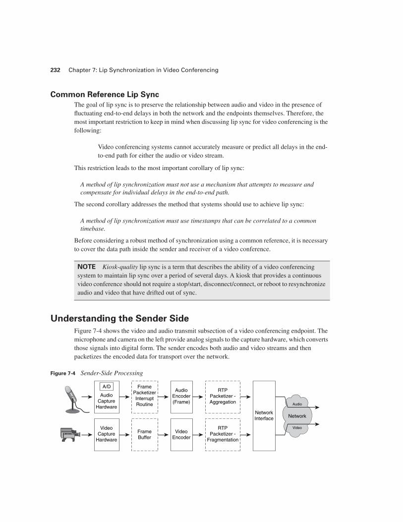
Figure 7-4 shows the video and audio transmit subsection of a video conferencing endpoint. The microphone and camera on the left provide analog signals to the capture hardware, which converts those signals into digital form. The sender encodes both audio and video streams and then packetizes the encoded data for transport over the network.

Figure 7-4 Sender-Side Processing

NOTE Kiosk-quality lip sync is a term that describes the ability of a video conferencing system to maintain lip sync over a period of several days. A kiosk that provides a continuous video conference should not require a stop/start, disconnect/connect, or reboot to resynchronize audio and video that have drifted out of sync.

Audio

NetworkNetworkInterface

A/D

AudioCapture

Hardware

Video

FramePacketizerInterruptRoutine

AudioEncoder(Frame)

FrameBuffer

VideoCapture

Hardware

VideoEncoder

RTPPacketizer -

Fragmentation

RTPPacketizer -Aggregation

Understanding the Sender Side 233

Sender Audio Path

This section focuses on the audio path, which uses an analog-to-digital (A/D) converter to capture analog audio samples and convert them into digital streams. For the purposes of synchronization, it is necessary to understand how each of the processing elements adds delay to the media stream.

The delays in the audio transmission path consist of several components:

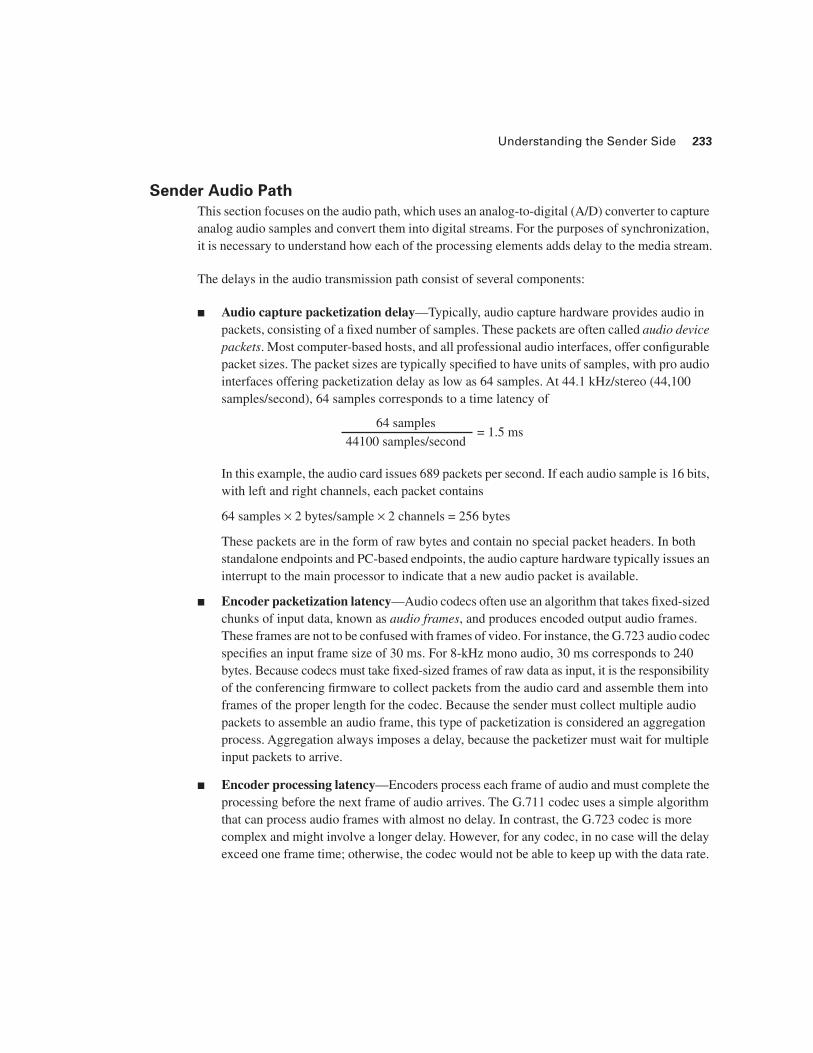
■ Audio capture packetization delay—Typically, audio capture hardware provides audio in packets, consisting of a fixed number of samples. These packets are often called audio device packets. Most computer-based hosts, and all professional audio interfaces, offer configurable packet sizes. The packet sizes are typically specified to have units of samples, with pro audio interfaces offering packetization delay as low as 64 samples. At 44.1 kHz/stereo (44,100 samples/second), 64 samples corresponds to a time latency of

In this example, the audio card issues 689 packets per second. If each audio sample is 16 bits, with left and right channels, each packet contains

64 samples × 2 bytes/sample × 2 channels = 256 bytes

These packets are in the form of raw bytes and contain no special packet headers. In both standalone endpoints and PC-based endpoints, the audio capture hardware typically issues an interrupt to the main processor to indicate that a new audio packet is available.

■ Encoder packetization latency—Audio codecs often use an algorithm that takes fixed-sized chunks of input data, known as audio frames, and produces encoded output audio frames. These frames are not to be confused with frames of video. For instance, the G.723 audio codec specifies an input frame size of 30 ms. For 8-kHz mono audio, 30 ms corresponds to 240 bytes. Because codecs must take fixed-sized frames of raw data as input, it is the responsibility of the conferencing firmware to collect packets from the audio card and assemble them into frames of the proper length for the codec. Because the sender must collect multiple audio packets to assemble an audio frame, this type of packetization is considered an aggregation process. Aggregation always imposes a delay, because the packetizer must wait for multiple input packets to arrive.

■ Encoder processing latency—Encoders process each frame of audio and must complete the processing before the next frame of audio arrives. The G.711 codec uses a simple algorithm that can process audio frames with almost no delay. In contrast, the G.723 codec is more complex and might involve a longer delay. However, for any codec, in no case will the delay exceed one frame time; otherwise, the codec would not be able to keep up with the data rate.

64 samples

44100 samples/second= 1.5 ms


■ RTP packetization delay—The RTP packetizer collects one or more audio frames from the encoder, composes them into an RTP packet with RTP headers, and sends the RTP packet out through a network interface. The packetization delay is the delay from the time the packetizer begins to receive data for the RTP packet until the time the RTP packetizer has collected enough audio frames to constitute a complete RTP packet. When an RTP packet is complete, the RTP packetizer forwards the packet to the network interface.

Both the packet size of encoded audio frames and the packet size of RTP packets impact delays on the sender side, for two reasons:

■ Whole-packet processing—Advanced audio codecs such as G.728 require access to the entire input frame of audio data before they can begin the encoding process. If a frame requires data from multiple audio device packets from the capture device, the audio codec must wait for a frame packetizer to assemble audio device packets into a frame before the encoder may begin the encode process. Lower-complexity codecs such as G.711 process audio in frames but do not need to wait for the entire frame of input data to arrive. Because the G.711 codec can operate on single audio samples at a time, it has a very low latency of only one sample.

■ RTP packetization delay—Even for encoders such as G.711 that have very low latency, RTP packetization specifies that encoded audio frames must not be fragmented across RTP packets. In addition, for more efficiency, an RTP packet may contain multiple frames of encoded audio. Because the RTP packetizer performs an aggregation step, it imposes a packetization delay.

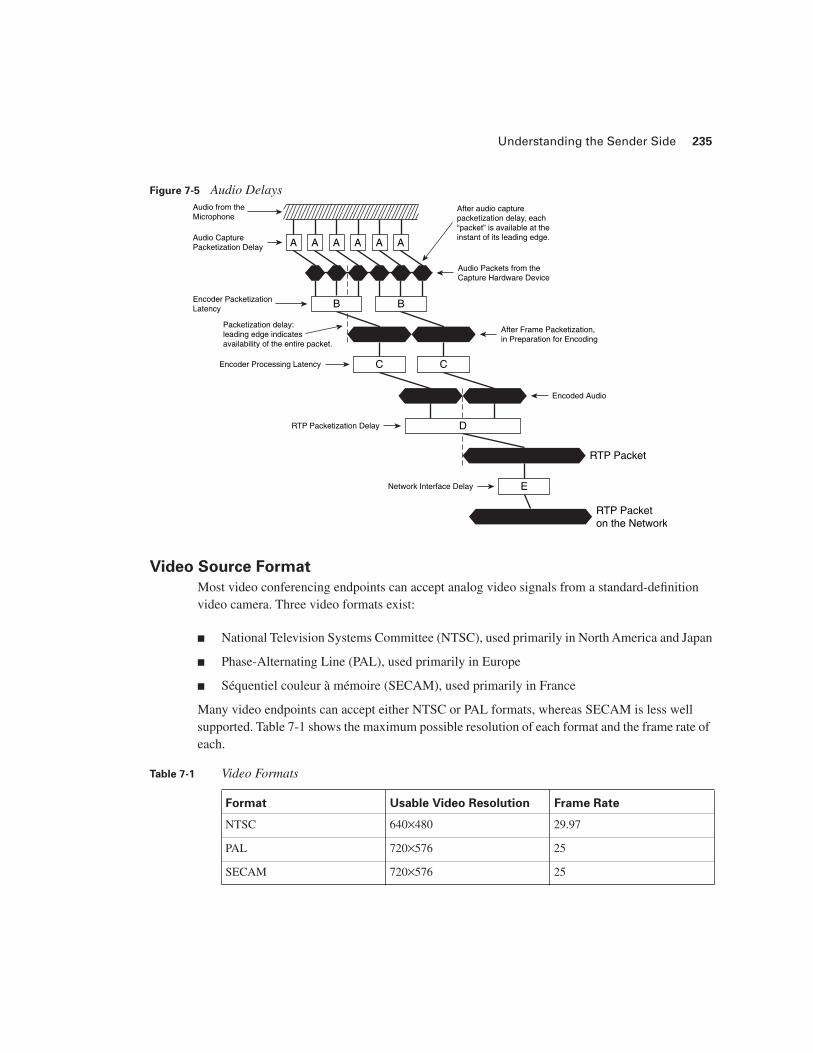
The final stage in the audio sender pipeline is the network interface, which receives packets from the RTP packetization stage and forwards them onto the network. The latency of the network interface is low compared to the other stages. To better show the delays in the transmit portion of the audio path, Figure 7-5 shows a timeline of individual delays.

Time is on the x-axis. In addition, the length of each packet in Figure 7-5 indicates the time duration of the data in the packet. In this figure, the entire packet or frame is available to the next processor in the chain as soon as the leading edge of that packet appears in the diagram. Figure 7-5 shows a common scenario in which successive processing steps perform packetization, increasing the packet size in later stages of the pipeline.


Figure 7-5 Audio Delays

Video Source Format

Most video conferencing endpoints can accept analog video signals from a standard-definition video camera. Three video formats exist:

■ National Television Systems Committee (NTSC), used primarily in North America and Japan

■ Phase-Alternating Line (PAL), used primarily in Europe

■ Séquentiel couleur à mémoire (SECAM), used primarily in France

Many video endpoints can accept either NTSC or PAL formats, whereas SECAM is less well supported. Table 7-1 shows the maximum possible resolution of each format and the frame rate of each.

Table 7-1 Video Formats

Format Usable Video Resolution Frame Rate

NTSC 640×480 29.97

PAL 720×576 25

SECAM 720×576 25

B B

C C

E

D

Audio from theMicrophone

Audio Packets from theCapture Hardware Device

After Frame Packetization,in Preparation for Encoding

Encoded Audio

RTP Packet

RTP Packeton the Network

Audio CapturePacketization Delay

RTP Packetization Delay

Network Interface Delay

Encoder PacketizationLatency

Encoder Processing Latency

Packetization delay:leading edge indicatesavailability of the entire packet.

After audio capturepacketization delay, each“packet” is available at the instant of its leading edge.

A A A A A A


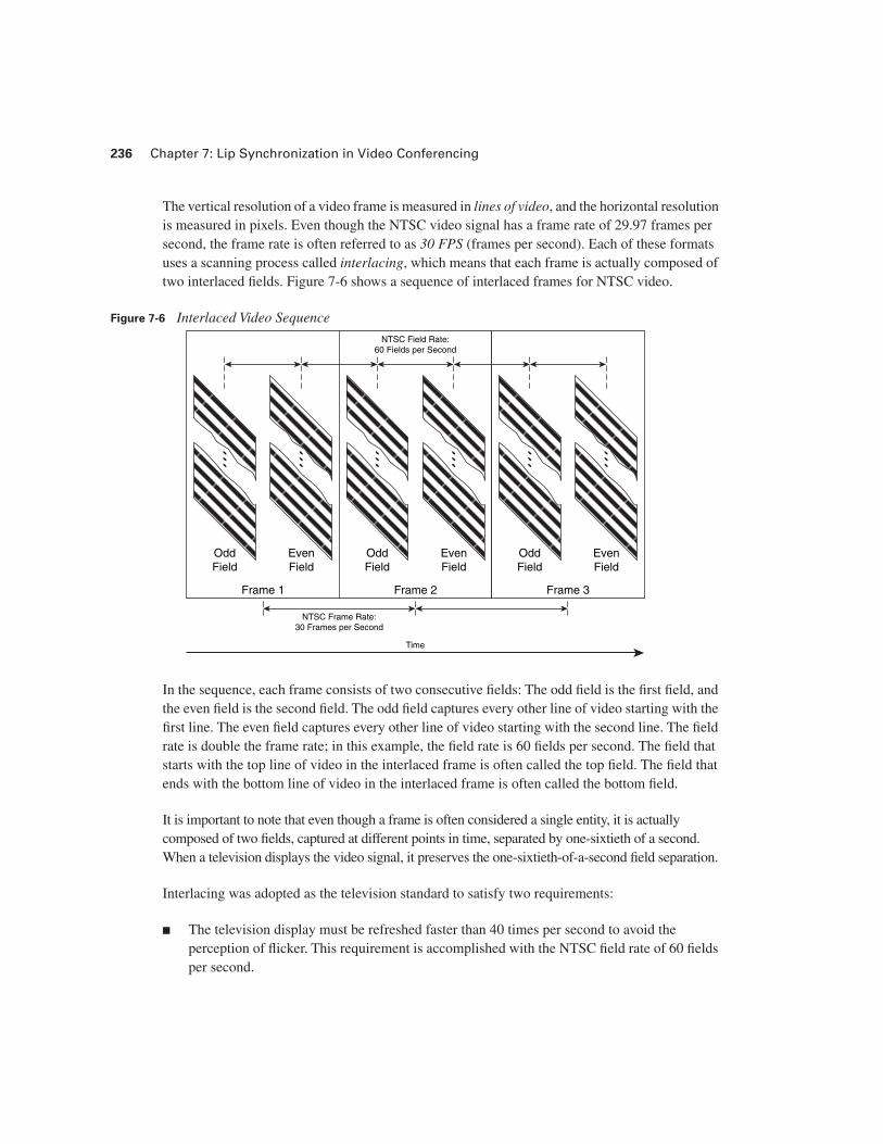
The vertical resolution of a video frame is measured in lines of video, and the horizontal resolution is measured in pixels. Even though the NTSC video signal has a frame rate of 29.97 frames per second, the frame rate is often referred to as 30 FPS (frames per second). Each of these formats uses a scanning process called interlacing, which means that each frame is actually composed of two interlaced fields. Figure 7-6 shows a sequence of interlaced frames for NTSC video.

Figure 7-6 Interlaced Video Sequence

In the sequence, each frame consists of two consecutive fields: The odd field is the first field, and the even field is the second field. The odd field captures every other line of video starting with the first line. The even field captures every other line of video starting with the second line. The field rate is double the frame rate; in this example, the field rate is 60 fields per second. The field that starts with the top line of video in the interlaced frame is often called the top field. The field that ends with the bottom line of video in the interlaced frame is often called the bottom field.

It is important to note that even though a frame is often considered a single entity, it is actually composed of two fields, captured at different points in time, separated by one-sixtieth of a second. When a television displays the video signal, it preserves the one-sixtieth-of-a-second field separation.

Interlacing was adopted as the television standard to satisfy two requirements:

■ The television display must be refreshed faster than 40 times per second to avoid the perception of flicker. This requirement is accomplished with the NTSC field rate of 60 fields per second.

OddField

EvenField

Frame 1

OddField

EvenField

Frame 2

NTSC Field Rate:60 Fields per Second

OddField

EvenField

Frame 3

NTSC Frame Rate:30 Frames per Second

Time


■ Bandwidth must be conserved. This requirement is satisfied by transmitting only half the frame content (every other line of video) for each refresh of the television display.

A video endpoint can process standard video for low-resolution or high-resolution conferencing, but the approach taken for each differs significantly.

Low-Resolution Video Input

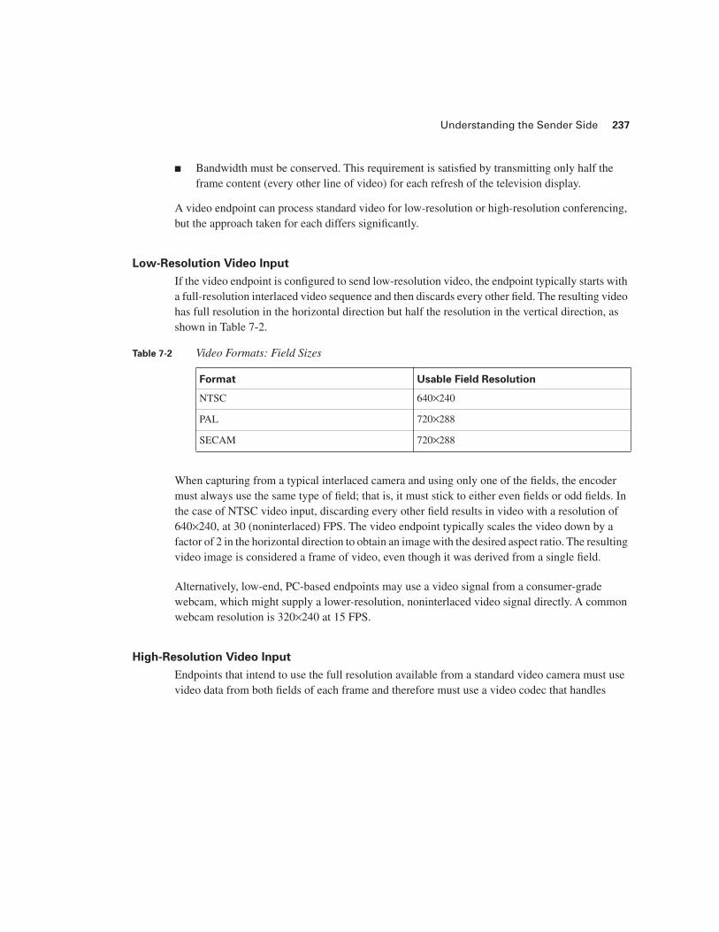
If the video endpoint is configured to send low-resolution video, the endpoint typically starts with a full-resolution interlaced video sequence and then discards every other field. The resulting video has full resolution in the horizontal direction but half the resolution in the vertical direction, as shown in Table 7-2.

When capturing from a typical interlaced camera and using only one of the fields, the encoder must always use the same type of field; that is, it must stick to either even fields or odd fields. In the case of NTSC video input, discarding every other field results in video with a resolution of 640×240, at 30 (noninterlaced) FPS. The video endpoint typically scales the video down by a factor of 2 in the horizontal direction to obtain an image with the desired aspect ratio. The resulting video image is considered a frame of video, even though it was derived from a single field.

Alternatively, low-end, PC-based endpoints may use a video signal from a consumer-grade webcam, which might supply a lower-resolution, noninterlaced video signal directly. A common webcam resolution is 320×240 at 15 FPS.

High-Resolution Video Input

Endpoints that intend to use the full resolution available from a standard video camera must use video data from both fields of each frame and therefore must use a video codec that handles

Table 7-2 Video Formats: Field Sizes

Format Usable Field Resolution

NTSC 640×240

PAL 720×288

SECAM 720×288


interlaced video. When you are using video from an NTSC camera, endpoints that have an interlace-capable codec can support resolutions up to 640×480 at 60 fields per second.

Sender Video Path

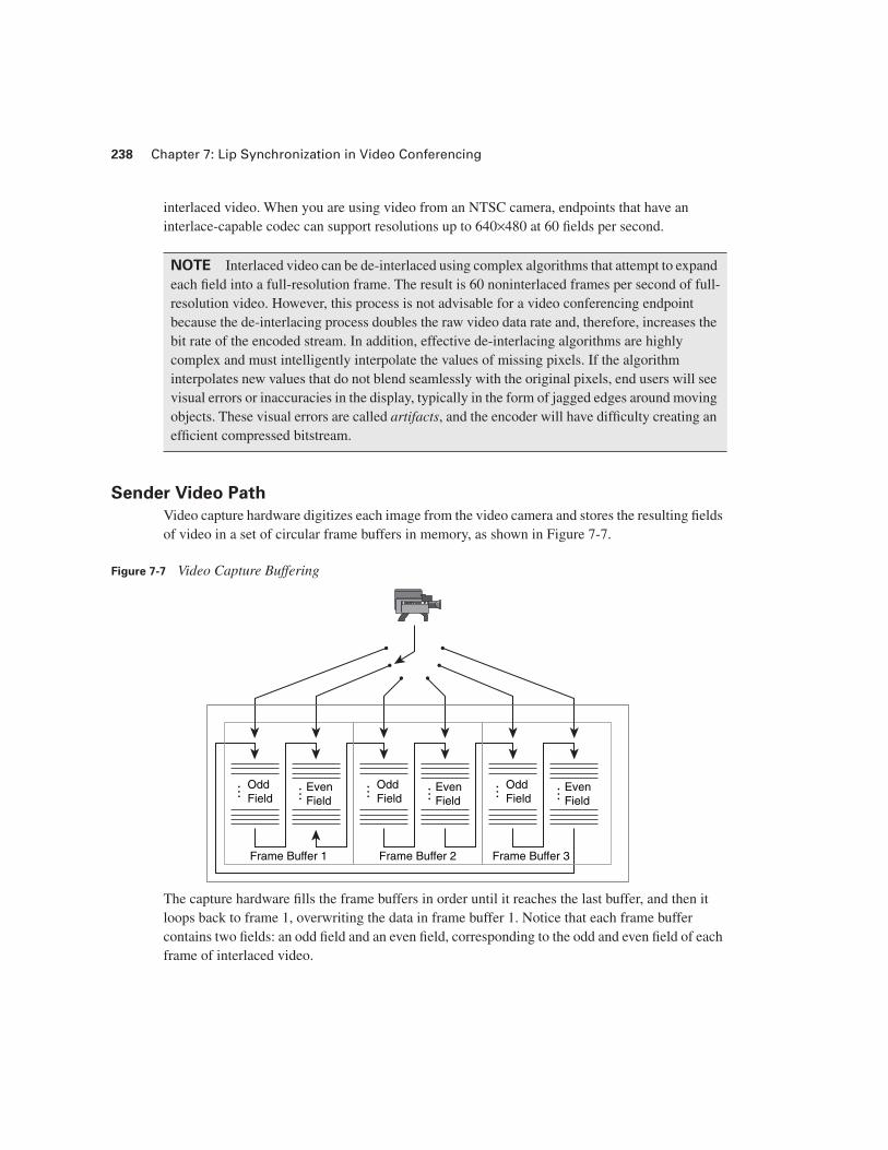
Video capture hardware digitizes each image from the video camera and stores the resulting fields of video in a set of circular frame buffers in memory, as shown in Figure 7-7.

Figure 7-7 Video Capture Buffering

The capture hardware fills the frame buffers in order until it reaches the last buffer, and then it loops back to frame 1, overwriting the data in frame buffer 1. Notice that each frame buffer contains two fields: an odd field and an even field, corresponding to the odd and even field of each frame of interlaced video.

NOTE Interlaced video can be de-interlaced using complex algorithms that attempt to expand each field into a full-resolution frame. The result is 60 noninterlaced frames per second of full-resolution video. However, this process is not advisable for a video conferencing endpoint because the de-interlacing process doubles the raw video data rate and, therefore, increases the bit rate of the encoded stream. In addition, effective de-interlacing algorithms are highly complex and must intelligently interpolate the values of missing pixels. If the algorithm interpolates new values that do not blend seamlessly with the original pixels, end users will see visual errors or inaccuracies in the display, typically in the form of jagged edges around moving objects. These visual errors are called artifacts, and the encoder will have difficulty creating an efficient compressed bitstream.

EvenField

EvenField

OddField

OddField

OddField

Frame Buffer 1 Frame Buffer 3Frame Buffer 2

… EvenField

… … … … …


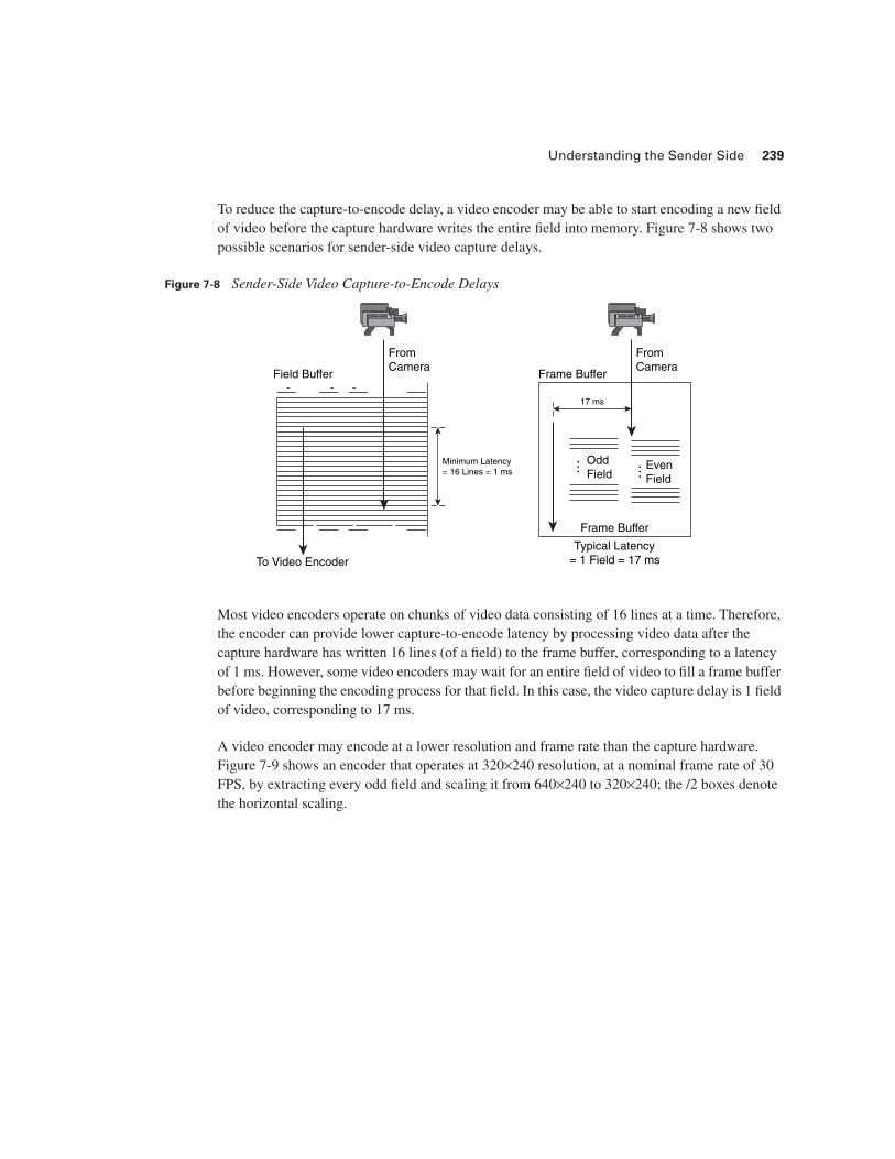
To reduce the capture-to-encode delay, a video encoder may be able to start encoding a new field of video before the capture hardware writes the entire field into memory. Figure 7-8 shows two possible scenarios for sender-side video capture delays.

Figure 7-8 Sender-Side Video Capture-to-Encode Delays

Most video encoders operate on chunks of video data consisting of 16 lines at a time. Therefore, the encoder can provide lower capture-to-encode latency by processing video data after the capture hardware has written 16 lines (of a field) to the frame buffer, corresponding to a latency of 1 ms. However, some video encoders may wait for an entire field of video to fill a frame buffer before beginning the encoding process for that field. In this case, the video capture delay is 1 field of video, corresponding to 17 ms.

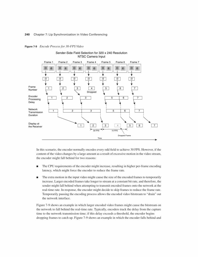
A video encoder may encode at a lower resolution and frame rate than the capture hardware. Figure 7-9 shows an encoder that operates at 320×240 resolution, at a nominal frame rate of 30 FPS, by extracting every odd field and scaling it from 640×240 to 320×240; the /2 boxes denote the horizontal scaling.

FromCamera

FromCamera

Field Buffer

To Video Encoder

Minimum Latency= 16 Lines = 1 ms

Frame Buffer

Frame Buffer

Typical Latency= 1 Field = 17 ms

17 ms

EvenField

OddField

… …


Figure 7-9 Encode Process for 30-FPS Video

In this scenario, the encoder normally encodes every odd field to achieve 30 FPS. However, if the content of the video changes by a large amount as a result of excessive motion in the video stream, the encoder might fall behind for two reasons:

■ The CPU requirements of the encoder might increase, resulting in higher per-frame encoding latency, which might force the encoder to reduce the frame rate.

■ The extra motion in the input video might cause the size of the encoded frames to temporarily increase. Larger encoded frames take longer to stream at a constant bit rate, and therefore, the sender might fall behind when attempting to transmit encoded frames onto the network at the real-time rate. In response, the encoder might decide to skip frames to reduce the frame rate. Temporarily pausing the encoding process allows the encoded video bitstream to “drain” out the network interface.

Figure 7-9 shows an example in which larger encoded video frames might cause the bitstream on the network to fall behind the real-time rate. Typically, encoders track the delay from the capture time to the network transmission time; if this delay exceeds a threshold, the encoder begins dropping frames to catch up. Figure 7-9 shows an example in which the encoder falls behind and

O E

/2

1

1

1

Frame 1

O E

/2

2

2

2

Frame 2

O E

/2

3

3

3

Frame 3

O E

/2

4

Dropped

FrameNumber

EncoderProcessingDelay

NetworkTransmissionDuration

Display atthe Receiver

30 FPS 15 FPS

Dropped Frame

Frame 4

Sender-Side Field Selection for 320 x 240 ResolutionNTSC Camera Input

O E

/2

5

5

5

Frame 5

O E

/2

6

6

6

Frame 6

O E

/2

7

1 2 3 4 5 6 7

7

7

Frame 7

Time

Understanding the Receive Side 241

decides to catch up by dropping the fourth output frame. Encoders routinely trade off between frame rate, quality, and bit rate in this manner.

Two delays exist in the video path on the capture side:

■ Video encoding delay—The encoding delay is the delay from the time that all data for a frame is captured until the time that the video encoder generates all encoded data for that frame. Video that contains large areas of motion might take longer to encode. In Figure 7-9, the latency of the encoder changes over time. However, despite the time-varying latency of the video encoder, the video stream is reconstructed on the receiver side with original uniform spacing.

■ RTP packetization delay—The RTP specification determines how the video bitstream must be spliced into RTP packets. Typically, video codecs divide the input image into sections, called slices, or groups of block (GOB). The RTP packetization process must splice the encoded bitstream at these boundary points. Therefore, the RTP video packetization must wait for a certain number of whole sections of the video bitstream to arrive to populate an RTP packet. The packetization delay is the time necessary for the packetizer to collect all data necessary to compose an RTP packet.

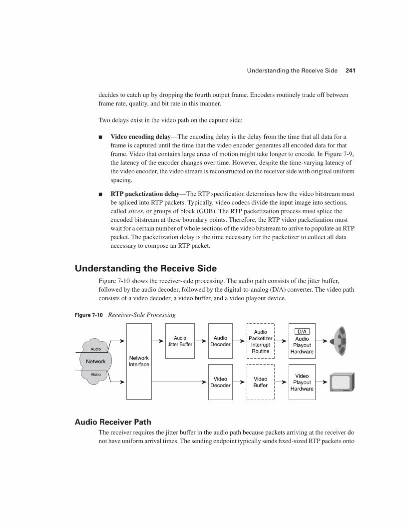
Understanding the Receive Side

Figure 7-10 shows the receiver-side processing. The audio path consists of the jitter buffer, followed by the audio decoder, followed by the digital-to-analog (D/A) converter. The video path consists of a video decoder, a video buffer, and a video playout device.

Figure 7-10 Receiver-Side Processing

Audio Receiver Path

The receiver requires the jitter buffer in the audio path because packets arriving at the receiver do not have uniform arrival times. The sending endpoint typically sends fixed-sized RTP packets onto

AudioJitter Buffer

AudioDecoder

AudioPacketizerInterruptRoutine

VideoDecoder

VideoBuffer

VideoPlayout

Hardware

AudioPlayout

Hardware

D/A

NetworkInterface

Audio

Network

Video


the network at uniform intervals, generating a stream with a constant audio bit rate. However, jitter in the network due to transient delays causes nonuniform spacing between packet arrival times at the receiver. If the network imposes a temporary delay on a sequence of several packets, those packets arrive late, causing the jitter buffer on the receive side to decrease. The jitter buffer must be large enough to prevent the buffer from dropping to the point where it underflows. If the jitter buffer underflows, the audio device has no data to play out the audio speakers, and the user hears a glitch.

This scenario, in which the jitter buffer runs out of data for the audio playout device, is called audio starvation. Conversely, if the network then transfers these delayed packets in quick succession, the burst of packets causes the jitter buffer to rise back to its normal level quickly.

The jitter buffer absorbs these arrival-time variations; however, the jitter buffer imposes an additional delay in the end-to-end audio pipeline. This delay is equal to the average level of the jitter buffer, measured in milliseconds. Therefore, the goal of the receive endpoint is to establish a jitter buffer with the smallest average latency, which can minimize the probability of an audio packet dropout. The endpoint typically adapts the level of the jitter buffer over time by observing the recent history of jitter and increasing the average buffer level if necessary. In fact, if the jitter buffer underflows and results in a dropped packet, the receiver immediately reestablishes a new jitter buffer with a higher average level to accommodate greater variance.

When the jitter buffer underflows, the audio decoder must come to the rescue and supply a replacement for the missing audio packet. This replacement packet may contain audio silence, or it may contain audio that attempts to conceal the lost packet. Packet loss concealment (PLC) is the process of mitigating the loss of quality resulting from a lost packet. One common form of PLC is to just replay the most recent packet received from the network.

The series of audio processing units—including the input buffer, decoder, and playout device—can be considered a data pipeline, each with its own delay. To establish the initial jitter buffer level, the receiver must “fill the pipe” by filling the entire pipeline on the receive side until the audio “backs up” the pipeline to the input buffers and achieves the desired input buffer level.

In addition, the jitter buffer can provide the delay necessary to re-sort out-of-order packets.

The audio decode delay is analogous to the corresponding audio encoding delay on the sending side. The audio hardware playout delay on the receiver is analogous to the audio hardware capture delay on the sender.

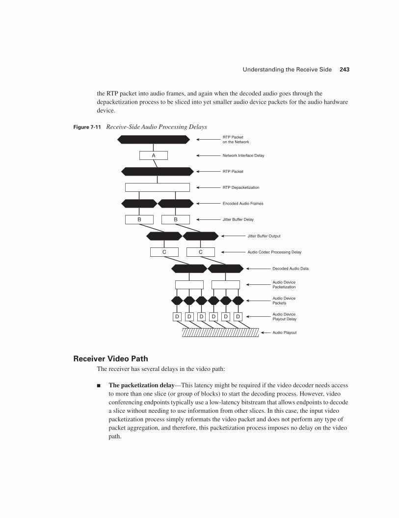
Figure 7-11 shows a graphical depiction of the delays on the receive side. When the receiver depacketizes a large packet into smaller packets, no delay results. The reason is because the receiver does not need to wait for successive packets of data to arrive, because depacketization does not perform an aggregation process. Such is the typical case when the receiver depacketizes

Understanding the Receive Side 243

the RTP packet into audio frames, and again when the decoded audio goes through the depacketization process to be sliced into yet smaller audio device packets for the audio hardware device.

Figure 7-11 Receive-Side Audio Processing Delays

Receiver Video Path

The receiver has several delays in the video path:

■ The packetization delay—This latency might be required if the video decoder needs access to more than one slice (or group of blocks) to start the decoding process. However, video conferencing endpoints typically use a low-latency bitstream that allows endpoints to decode a slice without needing to use information from other slices. In this case, the input video packetization process simply reformats the video packet and does not perform any type of packet aggregation, and therefore, this packetization process imposes no delay on the video path.

RTP Packet on the Network

Network Interface Delay

RTP Packet

RTP Depacketization

Encoded Audio Frames

Jitter Buffer Output

Audio Codec Processing Delay

Decoded Audio Data

Audio Device Packetization

Audio Device Packets

Audio Device Playout Delay

Audio Playout

Jitter Buffer Delay

A

B B

C C

D D D D D D


■ The decode delay—Analogous to the audio decode delay, it reconstructs slices of the video frame.

■ The synchronization delay—If necessary, the receiver may impose a delay on the video frames to achieve synchronization.

■ The playout delay—After the endpoint writes a new decoded video frame into memory, the playout delay is the time until that frame displays on the screen.

Types of Playout Devices

Playout devices come in two types: malleable and nonmalleable. Malleable playout devices can play a media sample on command, at any time. An example of a malleable playout device is a video display monitor. Typically, malleable devices do not request data; for instance, a receiver can send a video frame directly to the display device, and the device immediately writes the frame into video memory. The video frame appears on the screen the next time the TV raster scans the screen.

In contrast, nonmalleable devices always consume data at a constant rate. The audio playout device is an example: The receiver must move data to the audio device at exactly the real-time rate. Nonmalleable devices typically issue interrupt requests each time they must receive new data, and the receiver must service the interrupt request quickly to maintain a constant data rate to the device. After the receiver sends the first packet of audio to the audio device, the audio device typically proceeds to generate interrupt requests on a regular basis to acquire a constant stream of audio data. Audio devices generally receive fixed-size audio device packets of data at each interrupt, and professional audio interfaces can support buffer sizes as low as 64 samples. At 44.1 kHz and a 64-sample buffer size, packets will be 1.5 ms, and the audio device will generate about 689 interrupt requests per second.

RTP

The RTP specification RFC 3550 describes how senders can packetize and transmit media to receivers over the network. Using RTP packets alone, receivers can reconstruct and play audio and video streams from a sender and maintain continuous, glitch-free playback. However, to synchronize separate streams, senders and receivers must use RTCP packets, too. This section covers RTP packets for the purposes of unsynchronized stream playback, and the next section covers RTCP packets for the purposes of adding lip sync.

Canonical RTP Model

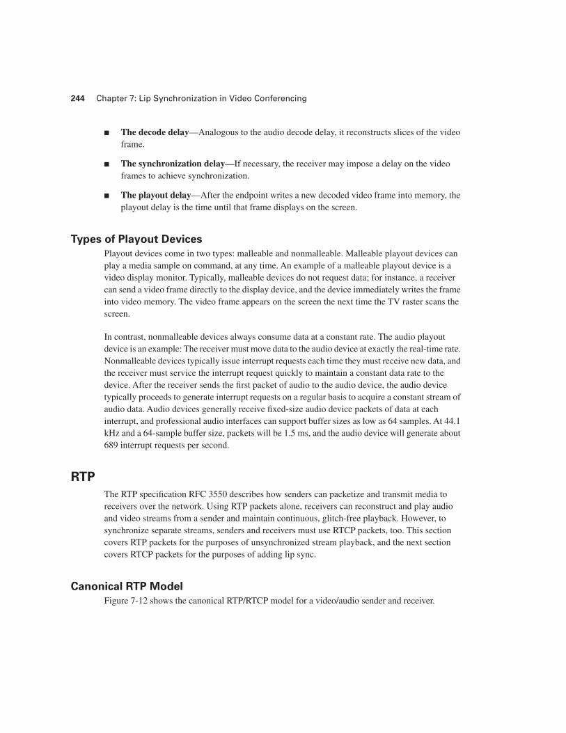
Figure 7-12 shows the canonical RTP/RTCP model for a video/audio sender and receiver.

RTP 245

Figure 7-12 Canonical RTP/RTCP Model

Figure 7-12 shows five different clocks.

At the sender

■ Clock A, used by the audio capture hardware to sample audio data

■ Clock B, used by the video capture hardware to sample video data

■ Clock C, the “common timebase” clock at the sender, used for the purposes of stream synchronization with RTCP packets

At the receiver

■ Clock D, the clock used by the audio playout hardware to play audio data

■ Clock E, the clock used by the video display hardware to display video data

A separate crystal oscillator drives each clock, which means that none of the clocks are synchronized to each other. In most video conferencing systems, the sender audio clock also provides the common timebase clock; however, this example considers the most general case, in which they differ.

SenderAudio RTPa

ReceiverAudio ATB

D

E

ReceiverVideo VTB

Video Frames

Audio Packets

SourceCapture

ReceiverPlayout

SenderVideo RTPv

SenderNTP

A

C

B

RTPa/ATBMapping

RTPv/VTBMapping

RTPa/NTPMapping

RTPv/NTPMapping


RTP Time Stamps

Each capture device (microphone and video capture hardware) has a clock that provides the RTP time stamps for its media stream. The units for the RTP time stamps depend on whether the media stream is audio or video:

■ For the audio stream, RTP uses a sample clock that is equal to the audio sample rate. For example, an 8-kHz audio stream uses a sample clock of 8 kHz. In this case, RTP time stamps for audio are actually sample stamps, because the time stamp can be considered a sample index. If an RTP packet has a time stamp of 0 and contains 300 samples, assuming the audio is continuous, the time stamp of the following RTP packet has an RTP time stamp of 300.

■ For video streams, RTP uses a sample clock equal to 90 kHz. For example, consider an endpoint that encodes a 25-FPS video sequence, derived by encoding every other field of PAL video: If a video frame consists of RTP packets with RTP time stamp 0, the next video frame consists of RTP packets with an RTP time stamp of 1/25 × 90000 = 3600. The sender may split a large encoded video frame into multiple RTP packets, in which case all RTP packets belonging to the same frame have the same RTP time stamp.

Remember that the RTP time stamps for the video stream and the audio stream are not related to each other. In particular, keep the following in mind:

■ The video and audio RTP time stamps do not begin transmission with the same RTP time stamp. According to the RTP specification, the sender must use a randomly selected beginning RTP time stamp for each stream to avoid known-value decryption attacks in case the endpoints encrypt the streams.

■ The crystal clocks on the audio capture hardware and video capture hardware are different (and therefore, unsynchronized).

Because the crystal clocks used for audio and video may differ, these clocks might drift past each other. Crystal clocks typically have an accuracy of ± 100 parts per million (ppm). As an example of clock drift, consider the following worst-case scenario:

■ If the audio clock is running at a frequency –100 ppm away from its nominal frequency, it is running .1 percent too slowly.

■ If the video clock is running at a frequency +100 ppm away from its nominal frequency, it is running .1 percent too fast.

In this example, the timebase of the video clock is fast relative to the timebase of the audio. Figure 7-13 shows how the timebases will crawl past each other over time.

RTP 247

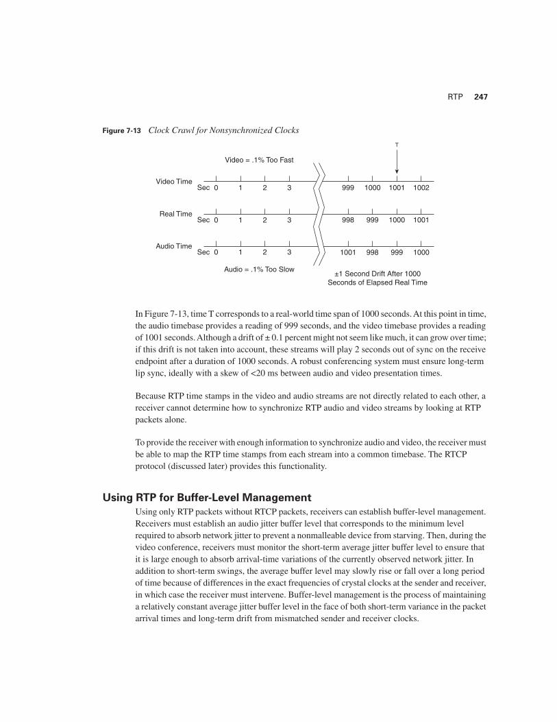
Figure 7-13 Clock Crawl for Nonsynchronized Clocks

In Figure 7-13, time T corresponds to a real-world time span of 1000 seconds. At this point in time, the audio timebase provides a reading of 999 seconds, and the video timebase provides a reading of 1001 seconds. Although a drift of ± 0.1 percent might not seem like much, it can grow over time; if this drift is not taken into account, these streams will play 2 seconds out of sync on the receive endpoint after a duration of 1000 seconds. A robust conferencing system must ensure long-term lip sync, ideally with a skew of <20 ms between audio and video presentation times.

Because RTP time stamps in the video and audio streams are not directly related to each other, a receiver cannot determine how to synchronize RTP audio and video streams by looking at RTP packets alone.

To provide the receiver with enough information to synchronize audio and video, the receiver must be able to map the RTP time stamps from each stream into a common timebase. The RTCP protocol (discussed later) provides this functionality.

Using RTP for Buffer-Level Management

Using only RTP packets without RTCP packets, receivers can establish buffer-level management. Receivers must establish an audio jitter buffer level that corresponds to the minimum level required to absorb network jitter to prevent a nonmalleable device from starving. Then, during the video conference, receivers must monitor the short-term average jitter buffer level to ensure that it is large enough to absorb arrival-time variations of the currently observed network jitter. In addition to short-term swings, the average buffer level may slowly rise or fall over a long period of time because of differences in the exact frequencies of crystal clocks at the sender and receiver, in which case the receiver must intervene. Buffer-level management is the process of maintaining a relatively constant average jitter buffer level in the face of both short-term variance in the packet arrival times and long-term drift from mismatched sender and receiver clocks.

Video = .1% Too Fast

Audio = .1% Too Slow

Video Time

Real Time

Audio Time

Sec 0 1 2 3

Sec 0 1 2 3

Sec 0 1 2 3

T

999 1000 1001 1002

998 999 1000 1001

1001 998 999 1000

±1 Second Drift After 1000Seconds of Elapsed Real Time


To achieve buffer-level management, receivers first establish a relationship between incoming RTP packets and the audio device timebase of the receiver as follows:

ATBout = RTPin + Krl

RTPin represents the RTP time stamp of the incoming packet, and ATBout represents the time stamp in the audio device timebase of the receiver. The audio device timebase of the receiver is defined by the audio device playout clock. Krl is an offset, chosen by the receiver, that maps one timebase into another. Both the RTP time stamp and the audio device timebase are in the same units, equal to the sample rate of the audio stream.

The audio playout device on the receiver typically operates using a pull model: After the receiver activates the audio device, the audio device starts issuing continual interrupt requests for data. The receiver responds to each interrupt by transferring data to the audio device. In this model, the audio playout device generates an interrupt to ask for audio and specifies the audio device time ATBout at which the audio must play. The receiver then uses Krl to calculate the corresponding RTPin RTP time stamp. The receiver must supply this data by retrieving it from the decoder, which in turn retrieves it from the jitter buffer. The value of Krl therefore enforces a mapping from RTP time stamp to audio device timebase, and the receiver must comply with this mapping.

The receiver establishes the value of Krl when the first RTP packet arrives. At this time, the receiver assigns a preliminary mapping from the RTP time stamp of the packet to the audio device timebase (ATB) of the receiver. This mapping achieves buffer management but not synchronization; the receiver must add delay to either the video or audio streams (discussed later) to achieve lip sync.

The receiver establishes the minimum Krl offset needed to satisfy jitter buffer level requirements. After the receiver selects Krl, it can set in motion the data pipeline for the audio stream.

The equation to calculate Krl uses several delay values, all of which are in units of the audio sample rate:

■ The current level of the jitter buffer is A. A will be nonzero if RTP packets have arrived before the receiver decides on a value of Krl.

■ The required nominal jitter buffer level is B.

■ The playout hardware delay is C.

■ The current audio device timebase time is D.

■ The RTP time stamp of the first RTP packet is RTPin1.

The RTP time stamp RTPin1 of the first RTP packet should be mapped to an audio device time ATB1 of

ATB1 = D + (B – A) + C

RTP 249

In other words, starting from the time right now, the stream must wait until its input buffer rises from its current level A to the desired nominal jitter buffer level B, which takes (B – A) units. The number of audio samples (B – A) represents the time during which the receiver “primes the input pipe” by filling the jitter buffer, which feeds the audio playout device. The (B – A) offset is required because the receive endpoint should not start playing audio through the audio playout device until the jitter buffer has achieved its nominal level. Alternatively, the receiver can supply initial silence audio to the audio playout device to quickly set the jitter buffer to its nominal level.

The receive endpoint estimates a desired value for B, based on the expected characteristics of the network packet jitter. A higher level of network jitter requires a larger input jitter buffer.

If more data has arrived than is needed to fill the jitter buffer to the required level, (B – A) will be negative. A negative value for (B – A) means that a portion of audio data at the beginning of the transmission must be discarded to reduce the jitter buffer to its nominal value.

The receiver logic must also take into account a delay of C through the playout hardware. For the audio playout device, the delay consists of the latency from the time the receiver passes a media packet to the playout hardware until the time the playout hardware passes the data to the D/A converter.

The preliminary offset Krl used for this mapping is as follows:

Krl = ATB1 – RTPin1 =D + (B – A) + C – RTPin1

The receiver now uses this value of Krl to map input RTP time stamps to time stamps in the audio device timebase. The receiver might need to change the level of the input buffer over time by changing the value of Krl. However, changing Krl causes the audio stream going to the playout device to be discontinuous. If the receiver increases Krl, the result is a gap in the audio stream, because the next packet plays at a later-than-normal time, and an intervening gap occurs; by default, the audio playout device is likely to fill this gap with silence. If the receiver decreases Krl, the result is an overlap in samples between the previous and next packet, which requires duplicate samples to be discarded. Gaps or discarded samples result in a glitch in the audio stream. However, the receiver can use two methods to change Krl while preventing an objectionable glitch:

■ The receiver can scale (stretch) the incoming audio data up or down by a small amount so that listeners will not notice the change. When decoded data is scaled up, the data rate entering the receiver effectively increases, and the jitter buffer level increases over time. The opposite effect occurs if the receiver scales down the input data. This method can be used to slowly change the jitter buffer level.


■ The receiver can wait for a duration of silence in the audio stream and then change Krl, which has the effect of increasing or decreasing the duration of silence. Listeners will not notice this change in the silence interval. This method can be used to abruptly change the jitter buffer level.

If the receiver does not require media synchronization, the only task left for the receiver is to manage the buffer level over time. The receiver can create a similar pipeline for video and perform the same type of buffer management. However, the video stream has the benefit of being a malleable medium, so the value of Krl can be changed on-the-fly without an objectionable glitch in the output. Another difference between the audio and video paths is this: The receiver typically measures the local video device timebase in units of seconds, instead of the RTP sample rate of 90 kHz.

Correlating Timebases Using RTCP

The RTCP protocol specifies the use of RTCP packets to provide information that allows the sender to map the RTP domain of each stream into a common reference timebase on the sender, called the Network Time Protocol (NTP) time. NTP time is also referred to as wall clock time because it is the common timebase used for all media transmitted by a sending endpoint. NTP is just a clock measured in seconds.

RTCP uses a separate wall clock because the sender may synchronize any combination of media streams, and therefore it might be inconvenient to favor any one stream as the reference timebase. For instance, a sender might transmit three video streams, all of which must be synchronized, but with no accompanying audio stream. In practice, most video conferencing endpoints send a single audio and video stream and often reuse the audio sample clock to derive the NTP wall clock. However, this generalized discussion assumes that the wall clock is separate from the capture clocks.

NTP

The wall clock, which provides the master reference for the streams on the sender endpoint, is in units of NTP time. However, it is important to bear in mind what NTP time is and what NTP time is not:

■ NTP time as defined in the RTP specification is nothing more than a data format consisting of a 64-bit double word: The top 32 bits represent seconds, and the bottom 32 bits represent fractions of a second. The NTP time stamp can therefore represent time values to an accuracy of ± 0.1 nanoseconds (ns).

■ The most widespread misconception related to the RTCP protocol is that it requires the use of an NTP time server to generate the NTP clock of the sender. An NTP time server provides a service over the network that allows clients to synchronize their clocks to the time server.

Correlating Timebases Using RTCP 251

The time server specifies that NTP time should measure the number of seconds that have elapsed since January 1, 1970. However, NTP time as defined in the RTP spec does not require the use of an NTP time server. It is possible for RTP implementations to use an NTP time server to provide a reference timebase, but this usage is not necessary and is out of scope of the RTP specification. Indeed, most video conferencing implementations do not use an NTP time server as the source of the NTP wall clock.

Forming RTCP Packets

Each RTP stream has an associated RTCP packet stream, and the sender transmits an RTCP packet once every few seconds, according to a formula given in RFC 3550. As a result, RTCP packets consume a small amount of bandwidth compared to the RTP media stream.

For each RTP stream, the sender issues RTCP packets at regular intervals, and those packets contain a pair of time stamps: an NTP time stamp, and the corresponding RTP time stamp associated with that RTP stream. This pair of time stamps communicates the relationship between the NTP time and RTP time for each media stream. The sender calculates the relationship between its NTP timebase and the RTP media stream by observing the value of the RTP media capture clock and the NTP wall clock in real time. The clocks have both an offset and a scale relationship, according to the following equation:

RTP/(RTP sample rate) = (NTP + offset) × scale

After determining this relationship by calculating the offset and scale values, the sender creates the RTCP packet in two steps:

1. The sender first selects an NTP time stamp for the RTCP packet. The sender must calculate this time stamp carefully, because the time stamp must correspond to the real-time value of the NTP clock when the RTCP packet appears on the network. In other words, the sender must predict the precise time at which the RTCP packet will appear on the network and then use the corresponding NTP clock time as the value that will appear inside the RTCP packet. To perform this calculation, the sender must anticipate the network interface delay.

2. After the sender determines the NTP time stamp for the RTCP packet, the sender calculates the corresponding RTP time stamp from the preceding relationship as follows:

RTP = ((NTP + offset) × scale) × sample_rate

The sender can now transmit the RTCP packet with the proper NTP and RTP time stamps.

NOTE In the RTP/RTCP protocol, the “NTP time” does not need to come from an NTP time server; the sender can generate it directly from any reference clock. Often, the sender reuses the audio capture clock as the basis for the NTP time.


Determining the values of offset and scale is nontrivial because the sender must figure out the NTP and RTP time stamps at the moment the capture sensor (microphone or camera) captures the data. For instance, to determine the exact point in time when the capture device samples the audio, the sender might need to take into account delays in the capture hardware. Typically, the audio capture device makes a new packet of audio data available to the main processor and then triggers an interrupt to allow the processor to retrieve the packet. When the sender processes an interrupt, the sender must calculate the NTP time of the first sample in each audio packet, corresponding to the moment in time when the sample entered the microphone. One method of calculating this time is by observing the time of the NTP wall clock and then subtracting the predicted latency through the audio capture hardware. However, a better way to map the captured samples to NTP time is for the capture device to provide two features:

■ A way for the sender to read the device clock of the capture device in real time, and therefore correlate the capture device clock to NTP wall clock time.

■ A way for the sender to correlate samples in the captured data to the capture device clock. The capture device can provide this functionality by adding its own capture device time stamp to each chunk of audio data.

From these two features, the sender can correlate audio samples to NTP wall clock time. The sender can then establish the relationship between NTP time and RTP time stamps by assigning RTP time stamps to the data.

The same principles apply to the video capture device. The sender must correlate a frame of video to the NTP time at which the camera CCD imager captures each field. The sender establishes the RTP/NTP mapping for the video stream by assigning RTP values to the video frames.

Using RTCP for Media Synchronization

The method of synchronizing audio and video is to consider the audio stream the master and to delay the video as necessary to achieve lip sync. However, this scheme has one wrinkle: If video arrives later than audio, the audio stream, not the video stream, must be delayed. In this case, audio is still considered the master; however, the receiver must first add latency to the audio jitter buffer to make the audio “the most delayed stream” and to ensure that synchronization can be achieved by delaying video, not audio.

NOTE The Microsoft DirectX streaming technology used for capture devices defines source filters, which are capture drivers that generate packets of captured data, along with time stamps. Hardware vendors write source filters for their capture hardware. Applications that use these source filters rely entirely on the source filters to provide data with accurate time stamps. If a source filter provides output streams for audio and video, it is critical that the source filter use kernel-level routines to ensure that the time stamps on the packets accurately reflect the time at which the hardware samples the media.

Correlating Timebases Using RTCP 253

In addition, the receiver must determine a relationship between the local audio device timebase ATB and the local video device timebase VTB on the receiver by calculating an offset AtoV:

VTB = ATB/(audio sample rate) + AtoV

This equation converts the local audio device timebase ATB into units of seconds by dividing the audio device time stamp by the audio sample rate. The receiver determines the offset AtoV by simultaneously observing Vtime, the value of the real-time video device clock, and Atime, the value of the real-time audio device clock. Then

AtoV = Vtime – ATime/(audio sample rate)

Now that the receiver knows AtoV, it can establish the final mapping for synchronization.

To establish this mapping, two criteria must be met:

■ At least one RTP packet must arrive from each stream.

■ The receiver must receive at least one RTCP packet for each stream, to associate each RTP timebase with the common NTP timebase of the sender.

For this method, the audio is the master stream, and the video is the slave stream. The general approach is for the receiver to maintain buffer-level management for the audio stream and to adapt the playout of the video stream by transforming the video RTP time stamp to a video device time stamp that properly slaves to the audio stream.

When a video frame arrives at the receiver with an RTP time stamp RTPv, the receiver maps the RTP time stamp RTPv to the video device time stamp VTB using four steps, as illustrated in Figure 7-14.

NOTE The Microsoft DirectX streaming technology used for playout devices defines render filters, which are essentially playback drivers that accept packets of data with time stamps that are relative to a global system time. The render filters play the media at the time indicated on the time stamp. Hardware vendors write filters for their playout hardware. Applications that use these render filters rely entirely on the render filters to play data accurately, based on the time stamps. A DirectX streaming render filter provides input connections in the form of input pins. If a render filter provides input pins for audio and video, it is critical that the render filter use kernel-level procedures to ensure that the time at which the hardware displays the media is accurately reflected by the time stamp on the packet.


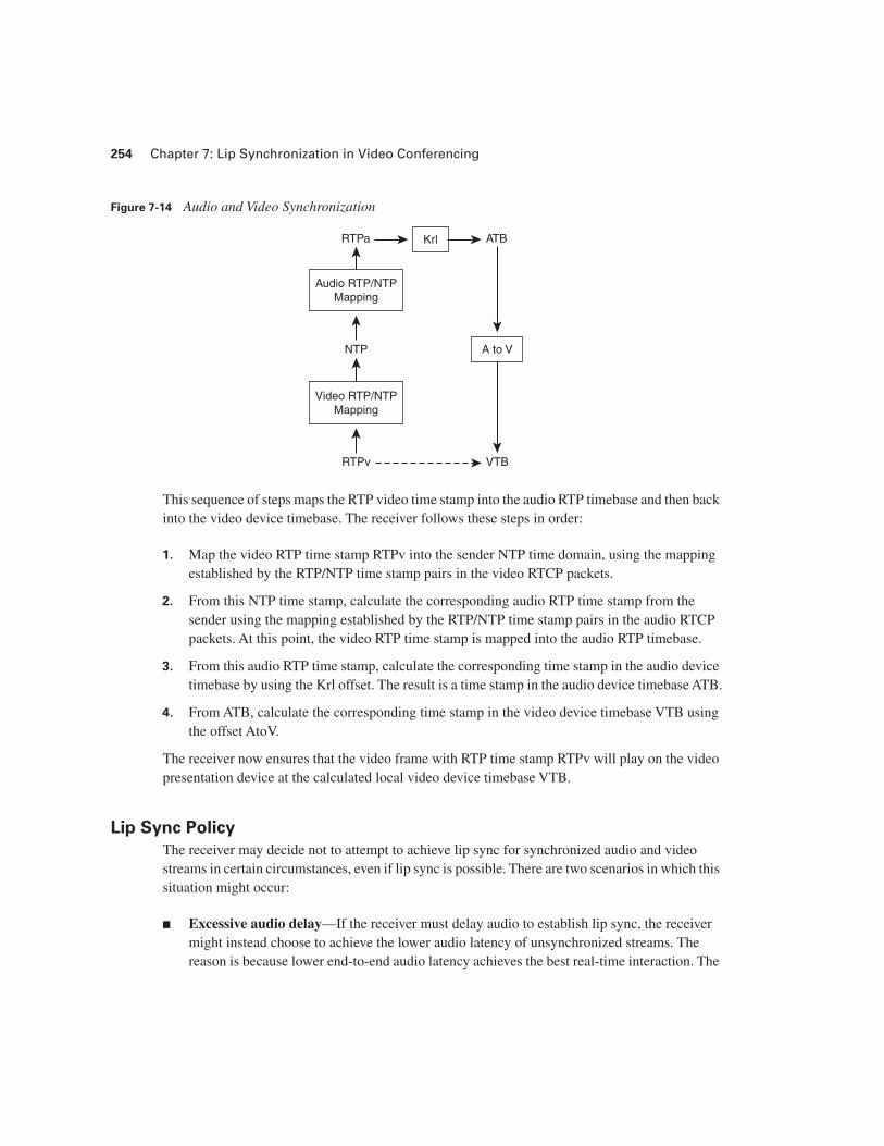
Figure 7-14 Audio and Video Synchronization

This sequence of steps maps the RTP video time stamp into the audio RTP timebase and then back into the video device timebase. The receiver follows these steps in order:

1. Map the video RTP time stamp RTPv into the sender NTP time domain, using the mapping established by the RTP/NTP time stamp pairs in the video RTCP packets.

2. From this NTP time stamp, calculate the corresponding audio RTP time stamp from the sender using the mapping established by the RTP/NTP time stamp pairs in the audio RTCP packets. At this point, the video RTP time stamp is mapped into the audio RTP timebase.

3. From this audio RTP time stamp, calculate the corresponding time stamp in the audio device timebase by using the Krl offset. The result is a time stamp in the audio device timebase ATB.

4. From ATB, calculate the corresponding time stamp in the video device timebase VTB using the offset AtoV.

The receiver now ensures that the video frame with RTP time stamp RTPv will play on the video presentation device at the calculated local video device timebase VTB.

Lip Sync Policy

The receiver may decide not to attempt to achieve lip sync for synchronized audio and video streams in certain circumstances, even if lip sync is possible. There are two scenarios in which this situation might occur:

■ Excessive audio delay—If the receiver must delay audio to establish lip sync, the receiver might instead choose to achieve the lower audio latency of unsynchronized streams. The reason is because lower end-to-end audio latency achieves the best real-time interaction. The

RTPa

RTPv

NTP

VTB

ATB

Audio RTP/NTPMapping

Video RTP/NTPMapping

Krl

A to V

References 255

receiver can make this determination after it achieves buffer management for both audio and video streams. If the audio stream is the most-delayed stream, the receiver can opt to delay the video stream to achieve lip sync; if the video stream is the most-delayed stream, however, the receiver might opt to avoid delaying audio to achieve lip sync.

■ Excessive video delay—If the receiver must delay video by a significant duration to achieve lip sync, on the order of a second or more, the receiver might need to store a large amount of video bitstream in a delay buffer. For high bit rate video streams, the amount of memory required to store this video data might exceed the available memory in the receiver. In this case, the receiver may opt to set an upper limit on the maximum delay of the video stream to accommodate the limited memory or forego video delay altogether.

Summary

This chapter covered several fundamental elements of a system that accurately achieves lip sync. The most important concept is this: The lip sync algorithm must depend on an absolute timebase instead of compensating for individual delays in the end-to-end path. To effectively use the NTP timebase as an absolute reference, the sender must establish accurate mappings between the NTP time and RTP media time stamps by sending RTCP packets for each media stream. The operation of the receiver consists of two phases: first, establishing buffer-level management for audio and video streams using only RTP time stamps, and then using NTP time to achieve synchronization. By maintaining absolute time references at both sender and receiver, audio and video remain in sync, even in the presence of variable delays in the end-to-end path.

References

ATSC Implementation Subcommittee Finding: “Relative Timing of Sound and Vision for Broadcast Operations,” Document IS-191 of the ATSC (Advanced Television Systems Committee), June 2003. www.atsc.org/standards/is_191.pdf

Blakowski and Steinmetz, “A Media Synchronization Survey: Reference Model, Specification, and Case Studies,” IEEE Journal on Selected Areas in Communications, Vol. 14, No. 1, January 1996.

Schulzrinne, H., S. Casner, R. Frederick, and V. Jacobson. IETF RFC 3550, RTP: A Transport Protocol for Real-Time Applications. July 2003.

Date post:	30-Apr-2018
Category:	Documents
Upload:	vothu
View:	231 times
Download:	2 times

Lip Synchronization in Video Conferencing -...

Documents