Office of Research & Library Services WSDOT Research Report Liquefacon-Induced Downdrag on Drilled Shaſts Balasingam Muhunthan Noel V. Vijayathasan Babak Abbasi WA-RD 865.1 April 2017 17-07-0293
Transcript
Office of Research & Library ServicesWSDOT Research Report
Liquefaction-Induced Downdrag on Drilled Shafts
Balasingam Muhunthan Noel V. VijayathasanBabak Abbasi
WA-RD 865.1 April 2017
17-07-0293
Research Report Agreement T4120, Task 26
WA-RD 865.1
LIQUEFACTION-INDUCED DOWNDRAG ON DRILLED SHAFTS by
Balasingam Muhunthan Noel V. Vijayathasan Babak Abbasi Principal Investigator
Department of Civil and Environmental Engineering
Washington State University Pullman, WA 99164-2910
Washington State Department of Transportation Technical Monitor
Tony Allen State Geotechnical Engineer
Prepared for
The State of Washington Department of Transportation
Roger Millar, Secretary
April 2017
1. REPORT NO. WA-RD 865.1
2. GOVERNMENT ACCESSION NO.
3. RECIPIENTS CATALOG NO
4. TITLE AND SUBTILLE Liquefaction-Induced Downdrag on Drilled Shafts
5. REPORT DATE April 2017
6. PERFORMING ORGANIZATION CODE
7. AUTHOR(S) Balasingam Muhunthan, Noel V. Vijayathasan and Babak Abbasi
8. PERFORMING ORGANIZATION REPORT NO.
9. PERFORMING ORGANIZATION NAME AND ADDRESS Washington State University Civil and Environmental Engineering Pullman, WA 99164-2910
10. WORK UNIT NO.
11. CONTRACT OR GRANT NO. Agreement T4120, Task 26
12. SPONSORING AGENCY NAME AND ADDRESS Washington State Department of Transportation Olympia Washington 98504-7370 Lu Saechao, Project Manager, 360-705-7260
13. TYPE OF REPORT AND PERIOD COVERED Final Research Report
14. SPONSORING AGENCY CODE
15. SUPPLEMENTARY NOTES This study was conducted in cooperation with the U.S. Department of Transportation, Federal Highway Administration.
16. ABSTRACT Sandy soil layers reduce in volume during and following liquefaction. The downward
relative movement of the overlying soil layers around drilled shafts induces shear stress along the shaft and changes the axial load distribution. Depending on the site conditions, the change in the axial responses that result from liquefaction-induced settlement and the drag load can have a significant impact on the performance of drilled shafts in seismic regions.
This study presents an analytical method to quantify the effects of liquefaction-induced downdrag on drilled shafts. The analytical method is based on the neutral plane method originally developed for clays but modified to account for liquefaction-induced effects. The neutral plane method is a simplification of soil-shaft interactions and is more representative of actual conditions compared to other methods. In this study, the neutral plane method was applied to an observed case of downdrag during the 8.8 magnitude earthquake in Maule, Chile and was able to predict the liquefaction-induced settlement that was the major cause of failure of the structure. The developed procedure is illustrated for two field cases of drilled shafts in liquefiable soils in Washington State. 17. KEY WORDS Axial loads, liquefaction-induced settlement, sand, seismic analysis, side resistance, soil liquefaction, soil settlement, drilled shafts
18. DISTRIBUTION STATEMENT No restrictions. This document is available to the public through the National Technical Information Service, Springfield, VA 22616
19. SECURITY CLASSIF. (of this report) None
20. SECURITY CLASSIF. (of this page) None
21. NO. OF PAGES 22. PRICE
Disclaimer
The contents of this report reflect the views of the authors, who are responsible for the
facts and the accuracy of the data presented herein. The contents do not necessarily reflect the
official views or policies of the Washington State Department of Transportation. This report does
not constitute a standard, specification, or regulation.
CHAPTER 3: MODIFIED UNIFIED METHOD FOR LIQUEFACTION-INDUCED DOWNDRAG: APPLICATION TO JUAN PABLO II BRIDGE ...............................................19
3.2 THE MODIFIED UNIFIED ANALYSIS METHOD FOR PILES (FELLENIUS AND SIEGEL 2008) ........................................................................................................................... 19
3.3 THE MODIFIED UNIFIED METHOD FOR DRILLED SHAFTS ................................... 23
3.3.1 STEP-BY-STEP ANALYSIS PROCEDURE FOR FURTHER MODIFICATION OF UNIFIED METHOD ............................................................................................................ 24
3.4 THE JUAN PABLO II BRIDGE CASE STUDY ............................................................... 34
3.4.1 FIELD OBSERVATIONS ........................................................................................... 36
3.4.3 LIQUEFACTION-INDUCED DOWNDRAG ANALYSIS BASED ON THE MODIFIED UNIFIED ANALYSIS METHOD FOR DRILLED SHAFTS ........................ 46
CHAPTER 4: LIQUEFACTION-INDUCED DOWNDRAG ANALYSIS: APPLICATION TO DRILLED SHAFTS IN BRIDGES IN WASHINGTON STATE ................................................55
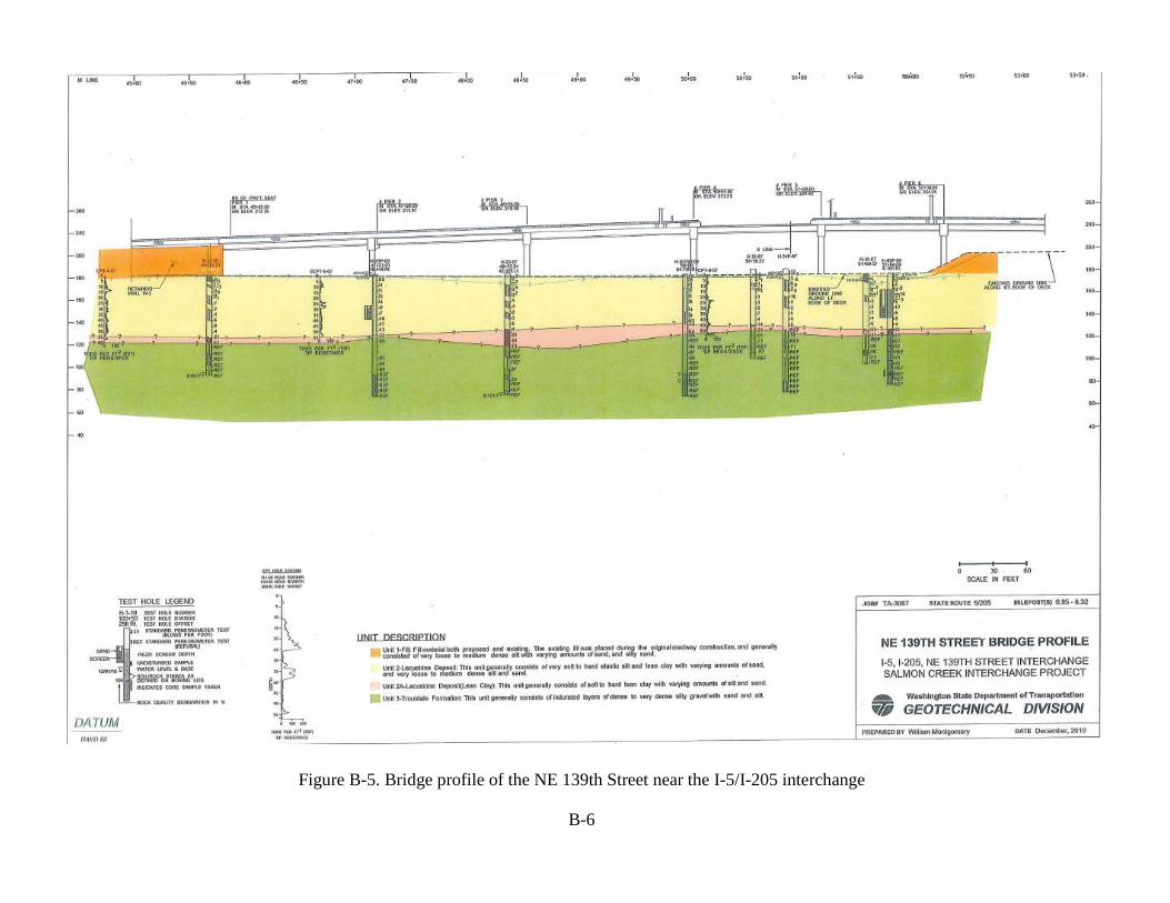
4.3 BRIDGE ON NE 139TH ST INTERCHANGE (I-5/I-205) ................................................. 65
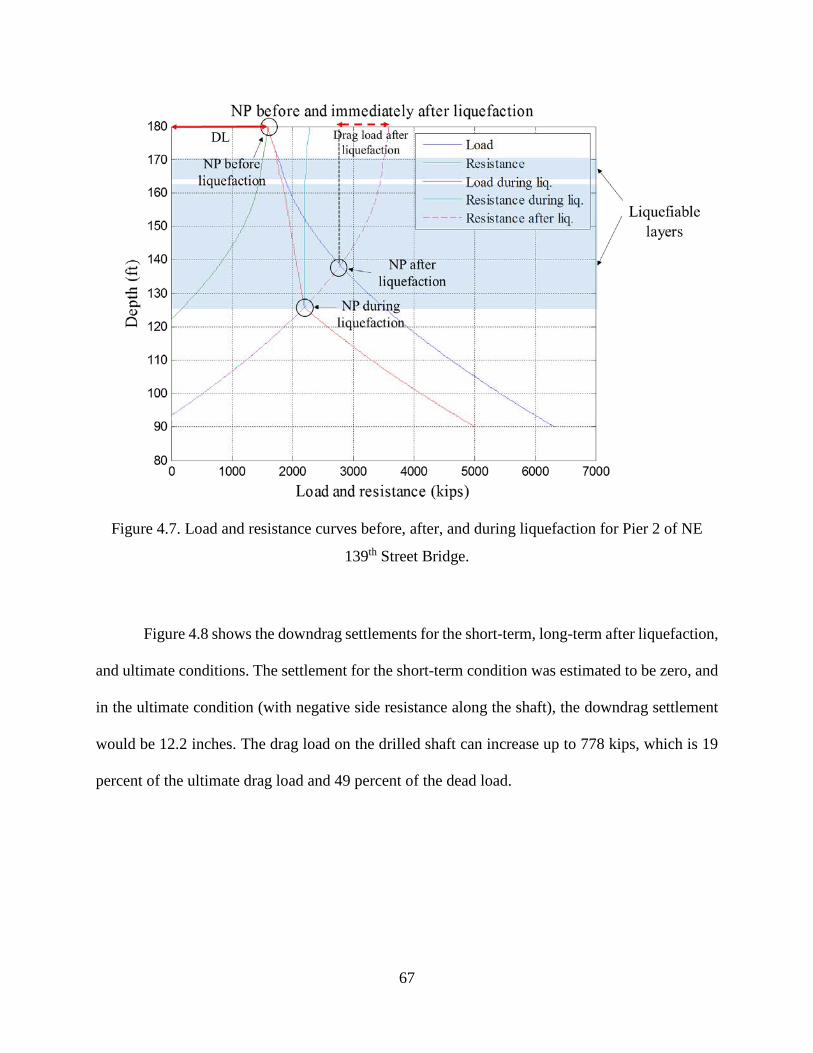
4. 4. DISCUSSION OF THE NEED TO ACCOUNT FOR 0.4 IN. DOWNDRAG BEFORE LIQUEFACTION (CASE II) .................................................................................................... 72
APPENDIX A: NUMERICAL ANALYSIS OF STRESS AND SETTLEMENT SOIL RESPONSES ...................................................................................................................................1
APPENDIX B: DOWNDRAG ANALYSIS FOR WSDOT CASE STUDIES ...............................1
APPENDIX C: NEUTRAL PLANE METHOD AND THE POSSIBLE NEED TO USE RESIDUAL STRENGTH IN LIQUEFIED LAYERS ....................................................................1
i
FIGURES
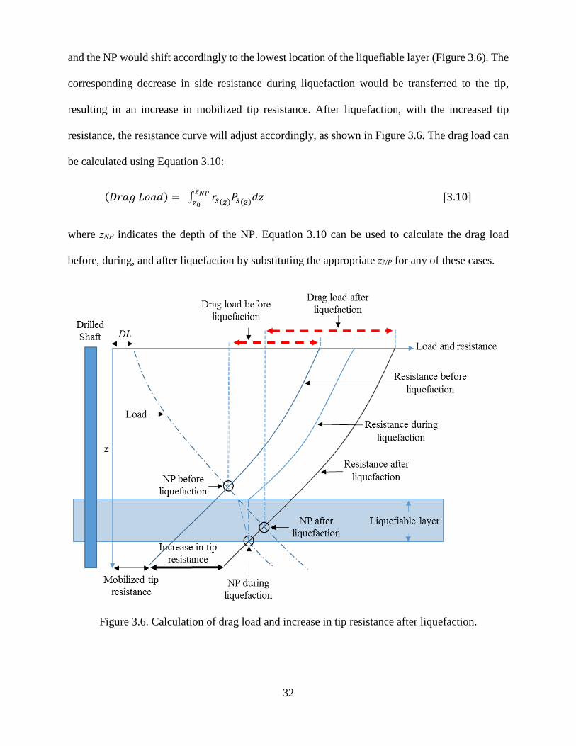
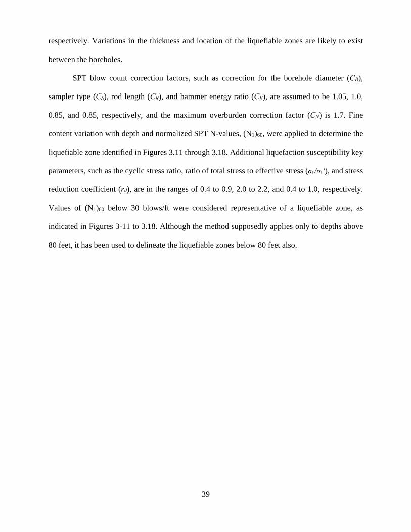
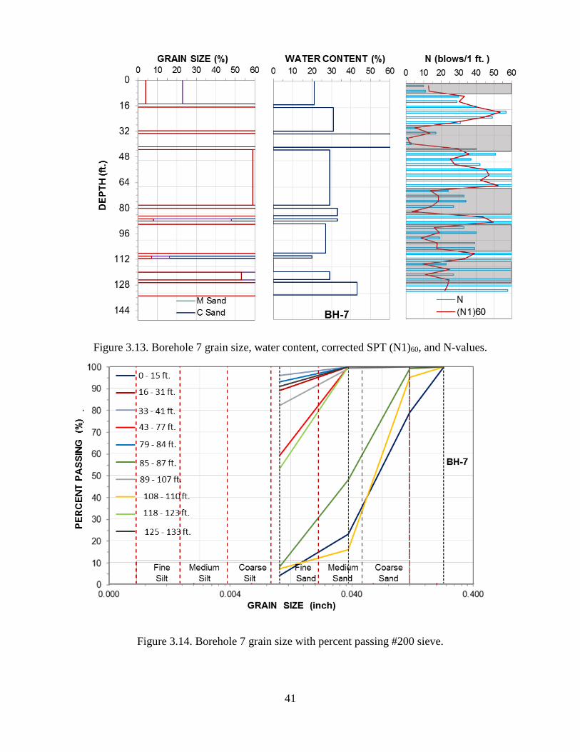
Figure 2.1. Stress distribution on a test pile (cE43) with time (Endo et al. 1969). ......................... 7 Figure 2.2. Comparison of soil and pile settlements for cE43 test pile with time (Endo et al. 1969). .............................................................................................................................................. 8 Figure 2.3. Variations within a liquefied layer: (a) excess pore pressure patterns (isochrones), (b) side resistance, (c) soil settlement, and (d) changing neutral plane location (Boulanger and Brandenberg 2004)........................................................................................................................ 10 Figure 2.4. Incremental liquefaction-induced downdrag (Boulanger and Brandenberg 2004). ... 12 Figure 2.5. Layout of test pile, instrumentation, and blast charges relative to the soil profile at the Massey Tunnel test site south of Vancouver, Canada (Rollins and Strand 2006). ....................... 14 Figure 2.6. Build-up and dissipation of excess pore pressure ratio (ru) at a depth of 8.4 m below the ground surface after detonation of explosive charges (Rollins and Strand 2006). ................. 14 Figure 2.7. Load distribution at the pile immediately before and immediately after blast-induced liquefaction and when the pore pressure had dissipated to essentially zero (Rollins and Strand 2006). ............................................................................................................................................ 15 Figure 2.8. Conceptual illustration of explicit method (Siegel et al. 2014). ................................. 17 Figure 3.1. Schematic diagram of location of neutral plane before liquefaction: (a) load and resistance curves and (b) soil and pile settlement curves. ............................................................ 20 Figure 3.2. Schematic diagram of typical responses when the liquefying zone is located above the neutral plane. ........................................................................................................................... 22 Figure 3.3. Schematic diagram of typical responses when the liquefying zone is located below the neutral plane. ........................................................................................................................... 23 Figure 3.4. Toe displacement response to end bearing load. The data points are from the curve suggested by O’Neill and Reese (1999), and the dotted curve is fitted to the data using Ratio Function (Fellenius 2014). ............................................................................................................ 27 Figure 3.5. Load and resistance curves derived from Equations 3.4 through 3.9. ........................ 31 Figure 3.6. Calculation of drag load and increase in tip resistance after liquefaction. ................. 32 Figure 3.8. (a) Column settlement under approach and (b) back face of failure plane at northern end of Juan Pablo II Bridge (Yen et al. 2011). ............................................................................. 35 Figure3.7. Google Earth view of Juan Pablo II Bridge location. .................................................. 36 Figure 3.9. Fine-grained material brought to the surface at Juan Pablo II Bridge (Bray and Frost 2010). ............................................................................................................................................ 37 Figure 3.11. Borehole 3 grain size, water content, corrected SPT (N1)60, and N-values with depth. ............................................................................................................................................. 40 Figure 3.12. Borehole 3 grain size with percent passing #200 sieve. ........................................... 40 Figure 3.13. Borehole 7 grain size, water content, corrected SPT (N1)60, and N-values. ............ 41 Figure 3.14. Borehole 7 grain size with percent passing #200 sieve. ........................................... 41 Figure 3.15. Borehole 10 grain size, water content, corrected SPT (N1)60, and N-values. .......... 42
Figure 3.16. Borehole 10 grain size with percent passing #200 sieve. ......................................... 42 Figure 3.17. Borehole 16 grain size, water content, corrected SPT (N1)60, and N-values. .......... 43
Figure 3.18. Borehole 16 grain size with percent passing #200 sieve. ......................................... 43 Figure 3.19. Post-liquefaction soil settlement profile near Boreholes 3, 7, 10, and 16 using the Tokimatsu and Seed (1987) procedure. ........................................................................................ 45
ii
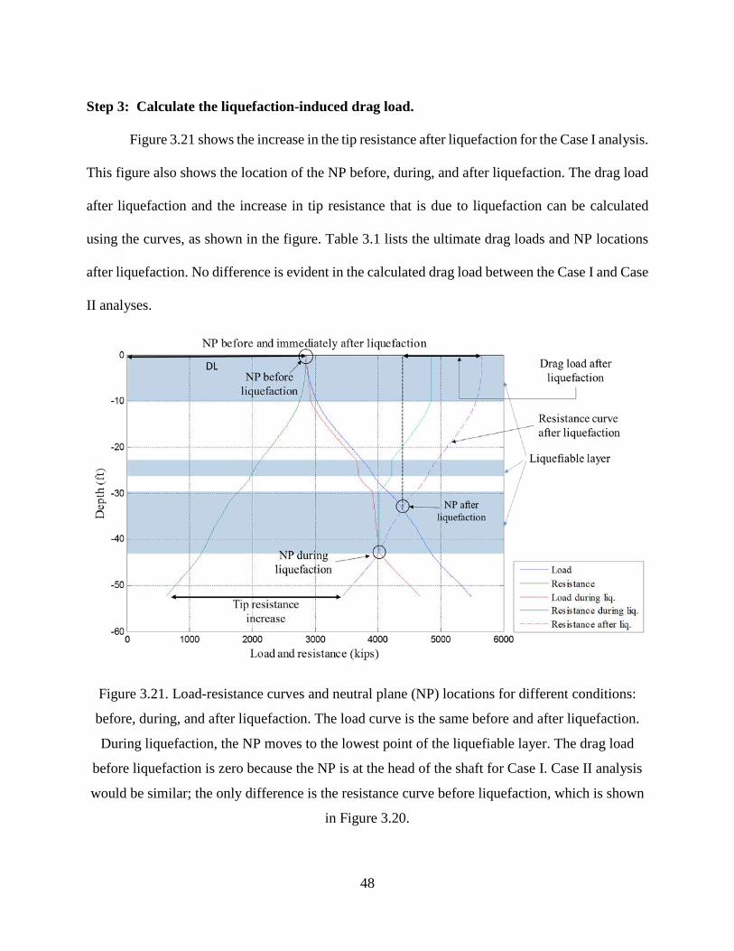
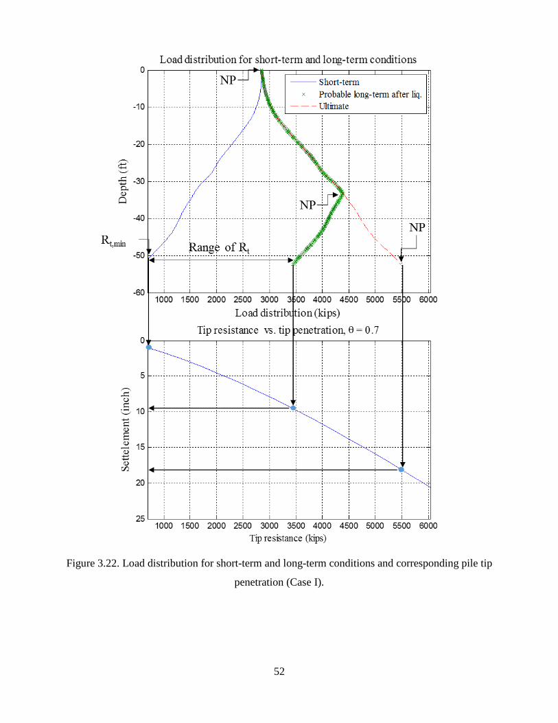
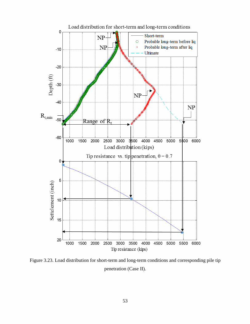
Figure 3.20. Load and resistance curves and neutral plane locations for drilled shafts before liquefaction for (a) Case I and (b) Case II analyses. The NP is located at the drilled shaft head for Case I analysis and at z = -5.4 ft for Case II analysis. .................................................................. 47 Figure 3.21. Load-resistance curves and neutral plane (NP) locations for different conditions: before, during, and after liquefaction. The load curve is the same before and after liquefaction. During liquefaction, the NP moves to the lowest point of the liquefiable layer. The drag load before liquefaction is zero because the NP is at the head of the shaft for Case I. Case II analysis would be similar; the only difference is the resistance curve before liquefaction, which is shown in Figure 3.20. ............................................................................................................................... 48 Figure 3.22. Load distribution for short-term and long-term conditions and corresponding pile tip penetration (Case I). ...................................................................................................................... 52 Figure 3.23. Load distribution for short-term and long-term conditions and corresponding pile tip penetration (Case II). .................................................................................................................... 53 Figure 4-1. Cross-section of ramp structure, soil profile, and location of piers for Talley Way interchange. ................................................................................................................................... 58 Figure 4.3. Load and resistance curves and neutral plane location for drilled shaft before liquefaction is assumed to occur at Pier 2 of the Talley Way interchange. The NP is located at the drilled shaft head before liquefaction. .......................................................................................... 61 Figure 4.4. The resistance curve is shown by the dashed line. The drag load before liquefaction is zero because the neutral plane is at the head of the shaft. ............................................................ 62 Figure 4.5. The load distribution (top) and downdrag settlements (bottom) for short-term, long-term after liquefaction, and ultimate conditions. .......................................................................... 64 Figure 4.6. NE 139th Street interchange (I-5/I-205). ..................................................................... 65 Figure 4.7. Load and resistance curves before, after, and during liquefaction for Pier 2 of NE 139th Street Bridge. ....................................................................................................................... 67 Figure 4.8. Load distribution and downdrag settlements for short-term, probable long-term after liquefaction, and ultimate conditions. ........................................................................................... 68 Figure 4.9. Downdrag settlements for short-term, long-term before and after liquefaction, and ultimate conditions for Pier 2 of the Talley Way interchange structure (Case II analysis). ......... 74 Figure 4.10. Load and resistance curves before, after, and during liquefaction for Pier 9 of NE 139th Street Bridge. All liquefiable layers are above the NP. ....................................................... 76 Figure 4.11. Load and resistance curves before, after, and during liquefaction for Pier 10 of NE 139th Street Bridge: (a) all liquefiable layers are considered to be liquefied and (b) the liquefiable layers above the neutral plane are not liquefied during an earthquake. ........................................ 78
iii
TABLES
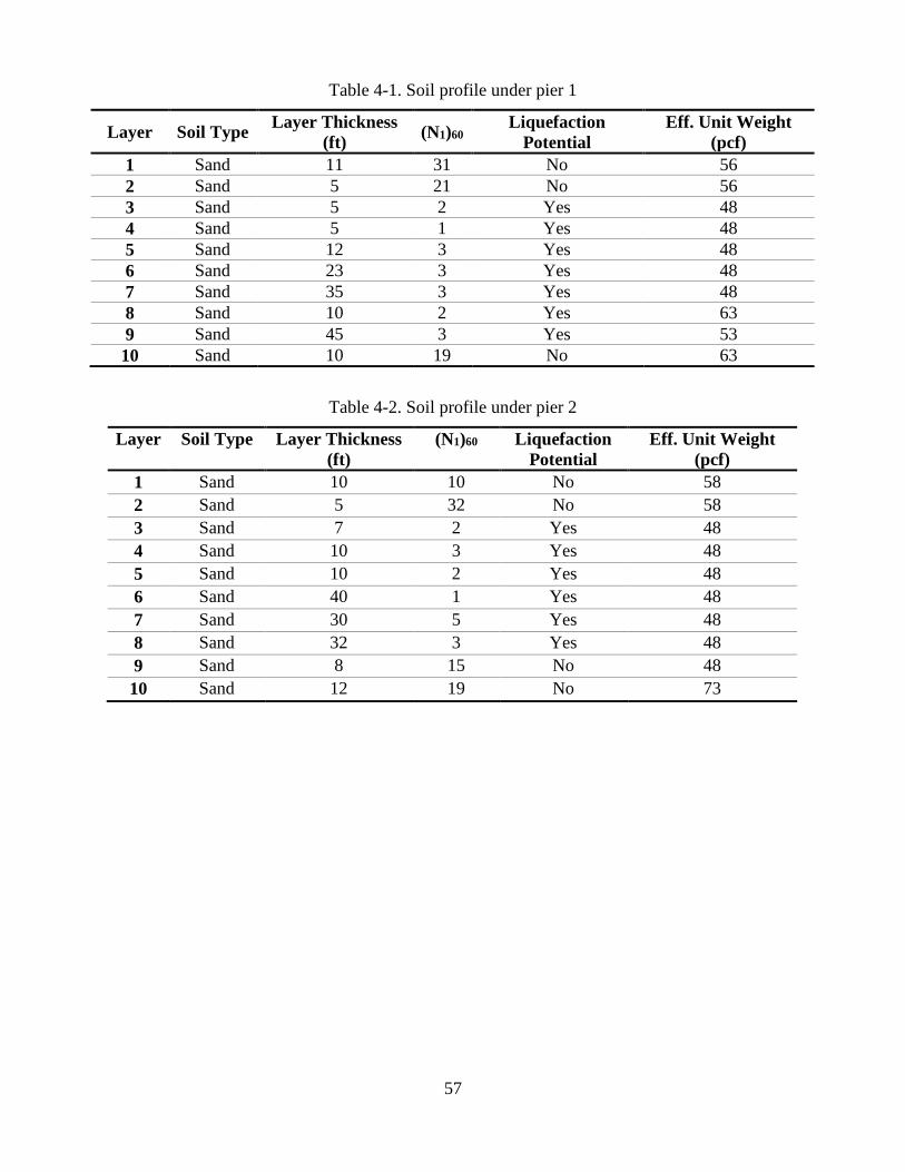
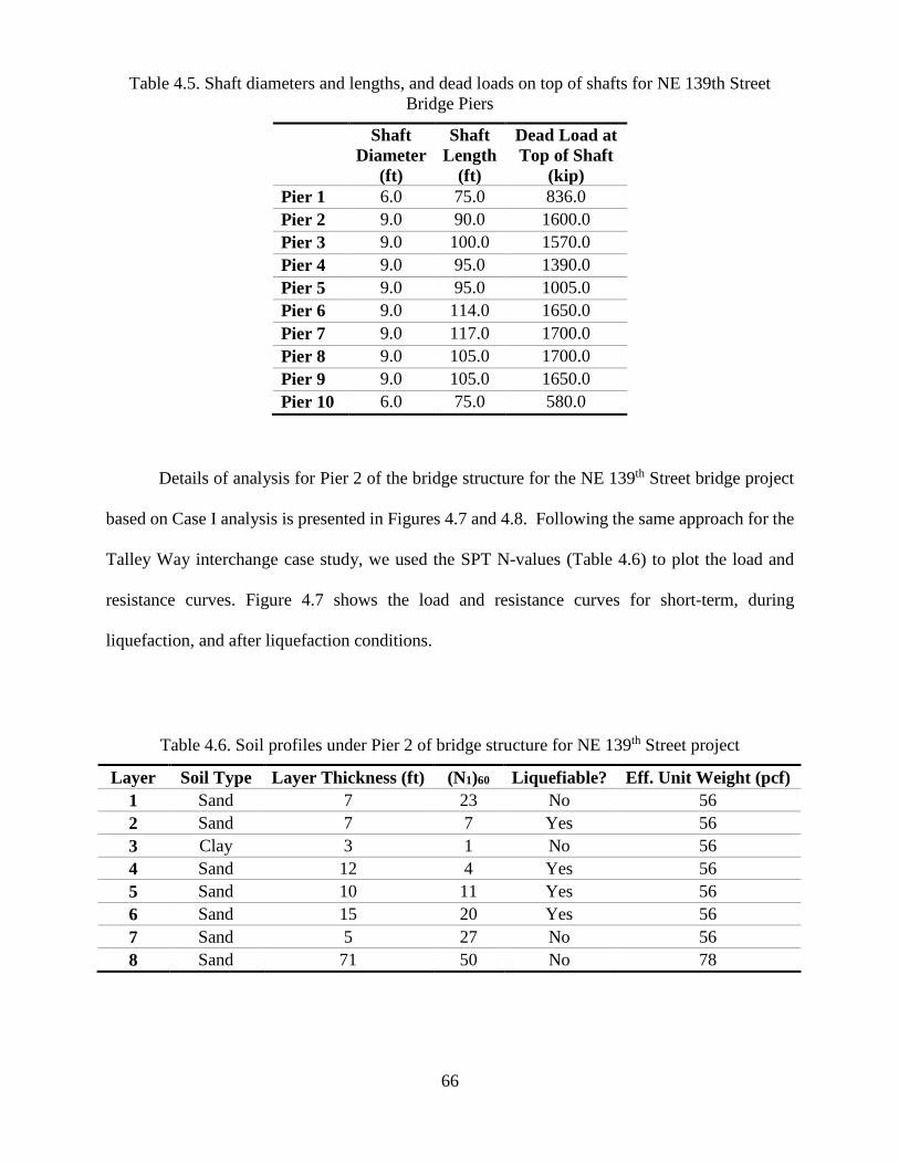
Table 3.1. Drag Loads for Pier 117 of Juan Pablo II Bridge ........................................................ 49 Table 3.2. Downdrag Settlements for Pier 117 Close to BH 3 ..................................................... 50 Table 3.3. Downdrag Settlements for Piers 1, 5, and 119 ............................................................ 54 Table 3.4. Drag Loads for Piers 1, 5, and 119 .............................................................................. 54 Table 4-1. Soil Profile under Pier 1 .............................................................................................. 57 Table 4-2. Soil Profile under Pier 2 .............................................................................................. 57 Table 4.3. Drag Loads for Talley Way Interchange Drilled Shafts .............................................. 62 Table 4.4. Downdrag Settlements for Talley Way Interchange Piers........................................... 63 Table 4.5. Shaft Diameters and Lengths, and Dead Loads on Top of Shafts for NE 139th Street Bridge Piers ................................................................................................................................... 66 Table 4.6. Soil Profiles under Pier 2 of Bridge Structure for NE 139th Street Bridge Project ..... 66 Table 4.7. Downdrag Settlements for NE 139th Street Project ..................................................... 70 Table 4.8. Drag Loads for NE 139th Street Project ....................................................................... 71 Table 4.9. Comparison of Liquefaction-Induced Downdrag Settlements and Drag Loads for Case (a) and Case (b) Analyses (Figure 4.11) ....................................................................................... 79 Table 4.10. Comparison of Liquefaction-Induced Drag Loads Obtained Using WSDOT Approach and Modified Unified Method ..................................................................................... 81
1
CHAPTER 1: INTRODUCTION
1.1 OVERVIEW
Drilled shafts often are used to transfer the structural loads to deeper firm strata. Load
transfer from shaft to soil or vice versa is accomplished by relative movement between shaft and
soil, which mobilizes shaft and tip resistances. The direction of side resistance depends on the
direction of the shaft movement. By definition, when the pile moves downward the resulting shear
stress along the shaft is in the upward direction, which is known as positive direction. The
downward relative movement of the soil around the shaft also induces shear stress along the shaft,
which is referred to as negative side resistance.
Sandy soil layers can reduce soil volume during and following liquefaction (Tokimatsu
and Seed 1987, Ishihara and Yoshimine 1992). The downward relative movement of the soil
around the shaft induces shear stress along the shaft commonly called negative side resistance. The
accumulated negative side resistance will affect the pile load and add axial force to the shaft, called
"drag force”.
Movement of the soil affects the load distribution along a drilled shaft. Depending on the
site conditions, the change in the axial responses that result from liquefaction-induced settlement
can have a significant impact on the performance of drilled shafts in seismic regions. In extreme
circumstances, the drag force may exceed the structural axial strength of the shaft. Other than for
very long piles (aspect ratio larger than about 100), the soil settlement around the pile will tend to
move the pile downward, i.e., add downdrag that may affect the serviceability of the structure.
Incidences of liquefaction-induced downdrag on piers and shafts that varied from near zero to
excessive amounts occurred February 27, 2010 during the 8.8 magnitude earthquake off the Maule
coast in central Chile (Yen et al. 2011).
2
Methods that often are employed to account for the effects of liquefaction on deep
foundations are addressed in terms of drag load development in design manuals, including the
American Association of State Highway and Transportation Officials (AASHTO) 2014 guidelines
and the Washington State Department of Transportation (WSDOT) 2015 guidelines. The AASHTO
(2014) specifications recommend adding the factored drag load from the soil layers above the
liquefiable zone to the factored loads from the superstructure. The AASHTO (2014) specifications
also contain simplified techniques to compute the drag load and recommend the use of non-
liquefied shaft resistance in the layers within and above the liquefied zone as well as shaft
resistance as low as the residual strength within the soil layers that do liquefy in order to estimate
the drag load for an extreme event limit state.
The development of drag load in piles and drilled shafts that have been constructed in
consolidating soils (i.e., under static loading) has been researched extensively for geotechnical
design. Different researchers have proposed several solutions to determine the magnitude and
distribution of drag loads that may act on piles in settling soils (e.g., Poulos and Davis 1990, Matyas
and Santamarina 1994, and Fellenius 1984, 2004). These studies present procedures to estimate the
forces and the location of the neutral plane (NP), which is the location along the pile where sustained
forces are in equilibrium with resisting forces (i.e., positive side resistance below the NP and
mobilized tip resistance).
Similarly, several researchers have proposed a number of numerical methods to account
for many of the features associated with drag load development (Lee and Ng 2004, Jeong et al.
2004, Hanna and Sharif 2006, Yan et al. 2012). These studies address the drag load that is caused
by a surcharge or consolidation of the surrounding soil. Wang and Brandenberg (2013) proposed
a method to estimate the pile response that is due to consolidation by applying a beam on a
nonlinear Winkler foundation using t-z elements to model the soil-pile interactions, with the pile
3
as the beam-column element. These researchers carried out their analysis using the finite element
code OpenSees (Open System for Earthquake Engineering Simulation) (2012) and provided an
estimate of the drag load by assuming that the relative velocity between the pile and the soil at the
NP is zero.
Unlike the number of studies of drag development in consolidating soils, only a few
analytical studies have addressed drag load and downdrag in cases where the soil settlement is caused
by seismic liquefaction (e.g., Boulanger and Brandenburg 2004, Rollins and Strand 2006, Fellenius
and Siegel 2008). For example, Boulanger and Brandenberg (2004) related the shaft resistance in
a reconsolidating liquefied zone to the dissipation of excess pore pressure over time and then
estimated the resulting drag load. In their study, downdrag was correlated incrementally over time
in parallel with the pore pressure dissipation. Also, Fellenius and Siegel (2008) applied the
concepts of ‘unified method’ (Fellenius 1984, 2004, 2014) to study the effects of seismic
liquefaction on downdrag. The unified method is based on the interaction between pile resistance
and soil settlement, notably the interaction between the pile tip resistance and pile tip penetration.
The method adopted by Fellenius and Siegel (2008) involves repositioning the NP based on the
location of a single liquefiable zone with respect to the original location, i.e., with the liquefiable
zone located above or below the NP. The validity of this approach has been demonstrated at a site
in northern California (Knutson and Siegel 2006) and in field tests by Rollins and Strand (2006)
and Strand (2008).
1.2 RESEARCH OBJECTIVES
The primary objective of this research is to develop an analytical method that can account
for liquefaction-induced downdrag (settlement) in deep foundations. The study includes a critical
examination of the existing analytical and numerical methods for downdrag analysis of piles and
4
drilled shafts. In this study, the NP method has been modified further to account for multiple layers
of liquefaction and applied to a case study of the 2010 earthquake off the Maule coast in Chile.
The analysis also identified the need to account for soil-structure interactions to better quantify the
effects of liquefaction-induced downdrag. Numerical simulations were performed using OpenSees
finite element software, which is widely used in earthquake engineering simulations (OpenSees
2014). The specific objectives of the study are to:
(i) Develop an analytical method to account for liquefaction-induced downdrag with regard to piles
and drilled shafts.
(ii) Verify the key assumptions made in (i) using OpenSees.
(iii) Evaluate the performance of selected drilled shafts in the State of Washington that are
vulnerable to liquefaction-induced downdrag during earthquakes.
1.3 OUTLINE OF REPORT
Chapter 1 provides an introduction to the concept of downdrag as it applies to deep
foundations and introduces the ideas used for the research conducted in this study. Chapter 2
presents a literature review of the current methods that pertain to liquefaction-induced downdrag.
Chapter 3 includes a review of the NP method and improvements and modifications to the method
for its application to liquefaction-induced downdrag. Also in Chapter 3, the modified NP method
is applied to study the observed settlement responses of piers along the Juan Pablo II Bridge during
the 2010 Maule 8.8 magnitude earthquake in Chile. Appendix A presents the numerical analysis
conducted using OpenSees to verify some of the key assumptions used in the analytical method.
Chapter 4 illustrates the developed procedure used to calculate downdrag for two field cases in the
State of Washington; these sites are potentially vulnerable to liquefaction. One of the field cases
5
is analyzed in detail, whereas the details relevant to the second case are presented in Appendix B
to ensure brevity of Chapter 4. Chapter 5 summarizes the study with conclusions and
recommendations for further advances in this research area.
6
CHAPTER 2: LITERATURE REVIEW
2.1 INTRODUCTION
When loose granular soils are saturated and subjected to strong ground shaking (repeated
loading or cyclic loading) under undrained conditions, the contractant behavior (reduction in
volume) of the soil layers causes pore pressure to accumulate, resulting simultaneously in the
reduction of effective stress. This reduction in effective stress progressively transfers granular soils
from a solid state to a liquefied state. In dense soils, such liquefaction leads to transient softening
and increased cyclic shear strain, dilatant behavior (expansion in volume) during shear induces
major strength loss and large ground deformations (Youd et al. 2001).
2.2 LIQUEFACTION-INDUCED DOWNDRAG
Sandy soil layers reduce the volume of the soil during and following liquefaction
(Tokimatsu and Seed 1987, Ishihara and Yoshimine 1992). This volume reduction manifests as a
downward movement, or settlement, of the overlying soil layers. Such movement may affect the
load distribution on deep foundations. Depending on the site conditions, the change in the axial
responses (i.e., drag load and downdrag) that result from liquefaction-induced settlement can have
a significant impact on the performance of piles or drilled shafts in seismic regions.
The development of drag load on piles and drilled shafts that have been constructed in
consolidating soils (i.e., under static loading) has been researched extensively for geotechnical
design. Researchers have proposed several solutions to determine the magnitude and distribution of
drag loads that may act on piles in settling soils (e.g., Poulos and Davis 1990, Matyas and
Santamarina 1994, and Fellenius 1984, 2004). These studies have proposed procedures to estimate
the forces and the location of the NP, i.e., the location along the pile where sustained forces are in
7
equilibrium with the resisting forces (i.e., positive side resistance below the NP and mobilized tip
resistance).
2.3 ENDO ET AL. (1969)
Endo et al. (1969) presented a case history that involves the behavior of the negative side
resistance on single piles installed in a clay medium. Measurements of side resistance for four
kinds of steel pipe piles, i.e., friction and point-bearing piles and open-point and closed-end pipe
piles, were taken for more than two years at a thick alluvial stratum where consolidation had been
observed due to a decrease in pore pressure. As shown in Figure 2.1, the observed load distribution
pattern indicates both positive side resistance and negative side resistance. Figure 2.2 presents the
measured soil and pile settlements. Endo et al. (1969) noted the existence of a NP, where the axial
stress in a pile is at a maximum level. The axial force due to the negative side resistance is
transmitted to the tip of pile while it is being diminished by the positive side resistance acting on
the pile below the neutral point.
Figure 2.1. Stress distribution on a test pile (cE43) with time (Endo et al. 1969).
8
Figure 2.2. Comparison of soil and pile settlements for cE43 test pile with time (Endo et al.
1969).
2.4 BOULANGER AND BRANDENBERG (2004)
Fellenius (1972) developed the NP method to estimate drag load and downdrag for piles in
clay. Boulanger and Brandenberg (2004) later modified the NP method for its application to
liquefaction-induced downdrag on vertical piles. This modified method accounts for the variation
in excess pore pressure (Δu) and ground settlement over time as a liquefied layer reconsolidates.
Sand compressibility (mv) and side resistance (fs) are considered as functions of the excess pore
pressure ratio. Drag load or side resistance in the consolidating soil will increase over time as the
effective stress increases (pore pressure decreases) during consolidation.
Sand compressibility, which depends on the excess pore pressure ratio (ru = u/σvo′ ), is used
to calculate soil settlement and pile head settlement as the liquefied layer reconsolidates. A
description of excess pore pressure isochrones over time and the relationship between mv and ru
9
are required to evaluate these settlements (Boulanger and Brandenberg 2004). Excess pore
pressure distribution patterns (isochrones) depend on the boundary and drainage conditions. The
isochrones may change according to the boundary conditions. The isochrones in the top liquefied
layer satisfy the test conditions whereas the bottom three liquefiable layers may not. The layers
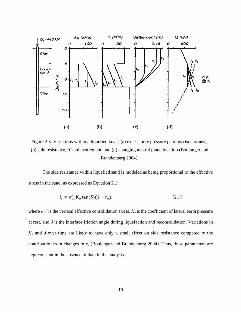
right above and below the liquefied layer affect the distribution pattern. Figure 2.3 (a) shows
typical excess pore pressure isochrones within a liquefied layer at different times (t0 – t3) during
reconsolidation. Here, t0 is the time immediately after ru = 100 percent, and t3 is the time that
corresponds to when Δu has fully dissipated. That is, the effective stress is almost zero at time t0
and is expected to reach a value at the end of primary consolidation. Florin and Ivanov (1961) also
observed a trapezoidal distribution of isochrones during their tests when the bottom soil layer and
the top layer are impermeable and permeable, respectively.
10
The side resistance within liquefied sand is modeled as being proportional to the effective
stress in the sand, as expressed as Equation 2.1:
fs = σvo′ Ko tan(δ)(1 − ru), [2.1]
where σvo' is the vertical effective consolidation stress, Ko is the coefficient of lateral earth pressure
at rest, and δ is the interface friction angle during liquefaction and reconsolidation. Variations in
Ko and δ over time are likely to have only a small effect on side resistance compared to the
contribution from changes in ru (Boulanger and Brandenberg 2004). Thus, these parameters are
kept constant in the absence of data in the analysis.
(a) (b) (c) (d)
Figure 2.3. Variations within a liquefied layer: (a) excess pore pressure patterns (isochrones),
(b) side resistance, (c) soil settlement, and (d) changing neutral plane location (Boulanger and
Brandenberg 2004).
11
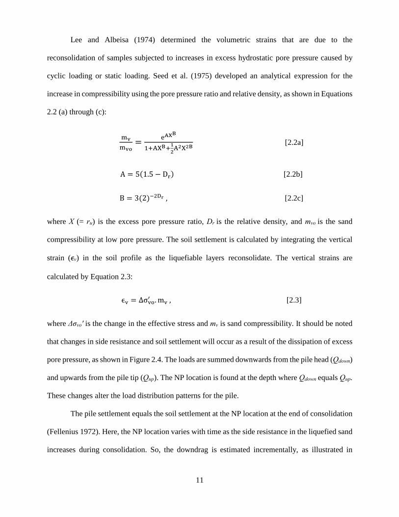
Lee and Albeisa (1974) determined the volumetric strains that are due to the
reconsolidation of samples subjected to increases in excess hydrostatic pore pressure caused by
cyclic loading or static loading. Seed et al. (1975) developed an analytical expression for the
increase in compressibility using the pore pressure ratio and relative density, as shown in Equations
2.2 (a) through (c):
mvmvo
= eAXB
1+AXB+12A2X2B
[2.2a]
A = 5(1.5 − Dr) [2.2b]
B = 3(2)−2Dr , [2.2c]
where X (= ru) is the excess pore pressure ratio, Dr is the relative density, and mvo is the sand
compressibility at low pore pressure. The soil settlement is calculated by integrating the vertical
strain (ϵv) in the soil profile as the liquefiable layers reconsolidate. The vertical strains are
calculated by Equation 2.3:
ϵv = Δσvo′ . mv , [2.3]
where Δσvo' is the change in the effective stress and mv is sand compressibility. It should be noted
that changes in side resistance and soil settlement will occur as a result of the dissipation of excess
pore pressure, as shown in Figure 2.4. The loads are summed downwards from the pile head (Qdown)
and upwards from the pile tip (Qup). The NP location is found at the depth where Qdown equals Qup.
These changes alter the load distribution patterns for the pile.
The pile settlement equals the soil settlement at the NP location at the end of consolidation
(Fellenius 1972). Here, the NP location varies with time as the side resistance in the liquefied sand
increases during consolidation. So, the downdrag is estimated incrementally, as illustrated in
12
Figure 2.4. For example, between times t2 and t3, the NP location moves upwards. The increment
of the pile settlement (ΔSpile) equals the increment of the soil settlement (ΔSsoil) at the NP location
at the end of this time step t3. Then, the total pile settlement is evaluated by numerically integrating
the increments of the pile settlement over the time for reconsolidation. This approach predicts
substantially smaller pile settlements for the end of the consolidation stage than the traditional NP
method.
2.5 ROLLINS AND STRAND (2006)
Rollins and Strand performed instrumented full-scale testing to investigate the loss of side
resistance, the development of negative side resistance, and the axial load distribution after blast-
Figure 2.4. Incremental liquefaction-induced downdrag (Boulanger and Brandenberg 2004).
13
induced liquefaction at a site near Vancouver, Canada. They measured these parameters before
and after the liquefaction event. The test pile was a 324-mm outside diameter steel pipe pile with
a 19-mm wall thickness that was driven close-ended to a depth of 21.3 m, as shown in Figure 2.5.
The soil profile consisted of clean sand, silty clay, and silty sand. A total of 16 explosive charges
at depths of 6.4 m and 8.5 m below the ground surface and equally spaced in a 10-m diameter
circle around the test pile were detonated sequentially with a one-second delay between
detonations to induce liquefaction. Figure 2.6 presents the recorded pore pressure measurements.
The settlement of the soil profile also was measured along with the pore pressure dissipation.
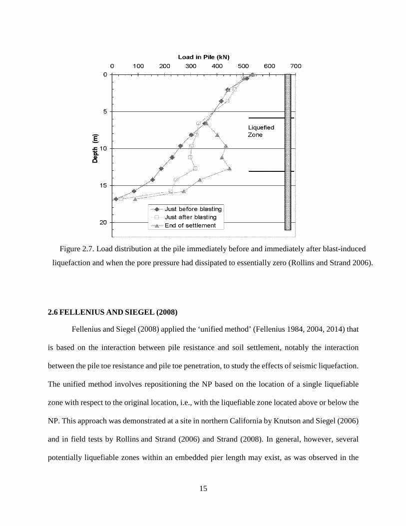
Figure 2.7 displays the axial load distribution on the pile immediately before and immediately after
blast-induced liquefaction and after the pore pressure had completely dissipated to zero. Figure 2.7
shows that the side resistance essentially reduced to zero around the liquefied zone as the excess
pore pressure ratio approached unity. As this layer settled due to the dissipation of the excess pore
pressure, negative side resistance developed with a unit value that was approximately half of the
positive side resistance prior to blasting. The soil settlement was about 270 mm. As a result of the
loss of the side resistance and then the downdrag load in the liquefied layer, the applied load was
transferred to the denser soil below the liquefied zone. The required displacement needed to
mobilize this additional side resistance was less than 10 mm (Rollins and Strand 2006). To the
author’s knowledge, this Rollins and Strand 2006 work is the only field test that has been
performed to date regarding liquefaction-induced downdrag and drag load.
14
Figure 2.5. Layout of test pile, instrumentation, and blast charges relative to the soil profile at the
Massey Tunnel test site south of Vancouver, Canada (Rollins and Strand 2006).
Figure 2.6. Build-up and dissipation of excess pore pressure ratio (ru) at a depth of 8.4 m below
the ground surface after detonation of explosive charges (Rollins and Strand 2006).
15
2.6 FELLENIUS AND SIEGEL (2008)
Fellenius and Siegel (2008) applied the ‘unified method’ (Fellenius 1984, 2004, 2014) that
is based on the interaction between pile resistance and soil settlement, notably the interaction
between the pile toe resistance and pile toe penetration, to study the effects of seismic liquefaction.
The unified method involves repositioning the NP based on the location of a single liquefiable
zone with respect to the original location, i.e., with the liquefiable zone located above or below the
NP. This approach was demonstrated at a site in northern California by Knutson and Siegel (2006)
and in field tests by Rollins and Strand (2006) and Strand (2008). In general, however, several
potentially liquefiable zones within an embedded pier length may exist, as was observed in the
Figure 2.7. Load distribution at the pile immediately before and immediately after blast-induced
liquefaction and when the pore pressure had dissipated to essentially zero (Rollins and Strand 2006).
16
case of the Maule, Chile earthquake. Such cases present the need to extend the recommendations
by Fellenius and Siegel (2008) to include multiple liquefiable zones, which forms the subject of
Chapter 3.
2.7 AASHTO METHOD
Methods that account for liquefaction effects on pile foundations are addressed in terms of
drag load development in a few design manuals, such as the AASHTO (2014) and WSDOT (2013)
specifications. The AASHTO (2014) specifications recommend adding the factored drag load from
the soil layers above the liquefiable zone to the factored loads from the superstructure. The AASHTO
(2014) specifications also contain simplified techniques to compute the drag load, recommending
the use of the non-liquefied side resistance in the layers within and above the liquefied zone and a
side resistance as low as the residual strength within the soil layers that do liquefy to estimate the
drag load for an extreme event limit state.
AASHTO (2014) also recommends using the ‘explicit method’ to calculate downdrag
instead of the NP method. Figure 2.8 describes the explicit method conceptually whereby the
negative side resistance is assumed to develop when the relative downward movement of the soil
is 0.4 inch or more. Hanningan et al. (2005) presented a step-by-step procedure for determining
the downdrag load; this procedure is based on the assumption that at least a 0.4-inch settlement
between the soil and the pile is needed to mobilize the negative side resistance. Along the shaft
where the settlement of the soil is more than 0.4 inch is assumed to have negative side resistance.
The drag load is applied as the top load after applying the appropriate load factor.
Siegal et al. (2014) compared the explicit and the NP analysis methods. The most important
difference between these two methods is the exclusion of the drag load at the geotechnical limit
17
state in the NP method. Siegal et al. (2014) also state that the NP method is a simplification of soil-
pile interaction and is more representative of actual pile conditions than the explicit method.
Figure 2.8. Conceptual illustration of explicit method (Siegel et al. 2014).
In summary, the experimental and field observation during the past decades urged the
geotechnical engineers to develop methods of downdrag analyses. These methods mostly involve
Ground settlement
0.4 in.
Positive side resistance
Negative side resistance
DD=Σ negative side resistance
18
the design at static loading conditions on piles in fine-grained soils (e.g. Boulanger and
Brandenberg 2004, and Fellenius 1972). Recently these methods are modified and applied for
liquefaction-induced downdrag analysis (e.g. Fellenius and Siegel 2008). Methods to account for
liquefaction-effects on deep foundations are also addressed in terms of drag load development in
a few design manuals, such as AASHTO (2014) and WSDOT (2015). In this study we further
modified the unified method by Fellenius and Siegel (2008) to be used for drilled shafts by
including their self-weight as well as the potential for the presence of multiple liquefiable layers.
This method is capable of predicting the downdrag settlement, drag load, and the axial load
distribution along the shaft, during and after the liquefaction, which gives a better understanding
of loads on the deep foundations compared to explicit methods addressed in design manuals.
19
CHAPTER 3: MODIFIED UNIFIED METHOD FOR LIQUEFACTION-INDUCED DOWNDRAG: APPLICATION TO JUAN PABLO II BRIDGE
3.1 INTRODUCTION
Fellenius and Siegel (2008) modified the original unified method (Fellenius 1984, 2004,
2014) for pile analysis to account for seismic liquefaction effects. The unified method is based on
the concept of the NP in piles and accounts for the interaction between pile resistance and soil
settlement, notably the interaction between the tip resistance and tip penetration. Fellenius and
Siegel’s modification for seismic liquefaction involves repositioning the NP based on the location
of a single liquefiable zone with respect to the original location, i.e., whether the liquefiable zone
is located above or below the NP. The validity of the approach has been demonstrated for a site in
northern California (Knutson and Siegel 2006) and in field tests by Rollins and Strand (2006) and
Strand (2008).
In the current study, this NP method has been extended further to include drilled shafts and
applied to the case of the pier performance at the Juan Pablo II Bridge during the Maule, Chile
earthquake in 2010 to verify its potential. Also in this study, numerical analyses were conducted
using OpenSees finite element software to examine some of the assumptions made in the study in
order to reinforce the study’s potential for applications to practice (see Appendix A).
3.2 THE MODIFIED UNIFIED ANALYSIS METHOD FOR PILES (FELLENIUS AND SIEGEL 2008)
Fellenius (1984, 1988, 2014) proposed the unified method to analyze the responses of deep
foundations to load and soil movement. This method makes use of the NP that relies on force and
settlement equilibria. The NP is located at the depth of the force equilibrium, i.e., where the load
and resistance curves intersect. The NP is also the plane where the soil and the pile both move
equally, i.e., the location of the settlement equilibrium.
20
Neutral Plane for Liquefied Soils
Figures 3.1 (a) and (b) show variations in the load and resistance curves and the pile and
settlement curves, respectively, in terms of depth along a pile before liquefaction. The NP is at the
intersection of the load and resistance curves.
The underlying principle of the load distribution curve is common for all conditions, i.e.,
before, during, and after liquefaction. The curve begins with the dead load, Qd, at the pile head and
increases with depth, assuming fully mobilized negative side resistance along the pile, with the
value Rs at the tip. The resistance curve initiates with the mobilized tip resistance, Rt, and increases
(b) SETTLEMENT
DEP
TH
(a) LOAD AND RESISTANCE
Potential liquefying layer
Neutral plane
Qd Qu
Rs Rt
Load curve
Pile settlement
Soil settlement
Figure 3.1. Schematic diagram of location of neutral plane before liquefaction: (a) load and
resistance curves and (b) soil and pile settlement curves.
Resistance curve
Axial force distribution
21
upward along the pile, thus corresponding to the fully mobilized positive side resistance and
attaining the value Qu. The load curve is not necessarily the actual load on the pile, but the potential
maximum load per depth if all the side resistance is dragging on the foundation. The resistance
curve is also the maximum available resistance distribution. The distribution of the axial force
along the pile (dashed line in Figure 3.1 (a)) follows the load distribution curve above the NP and
the resistance curve below the NP.
The liquefaction of a zone will result in (1) loss of effective stress, which indicates a
corresponding loss of side resistance, and (2) loss of volume, which indicates that the zone will
reduce in thickness and will potentially show up as settlement of the ground surface. Unless the
liquefiable portion of the soil profile is significant, the loss of the side resistance will be negligible.
The side resistance will be regained when the seismically imposed liquefaction effects have waned.
However, the loss of soil volume, i.e., settlement, may have a significant effect on the pile,
depending on whether or not the liquefiable zone is located above or below the NP, as explained
as follows.
a) If the liquefiable zone is located above the NP (Figure 3.2), then due to the unloading of
the pile, theoretically a small (hardly measurable) temporary elongation of the pile may
potentially appear as heave at the pile head. The load distribution curve will translate
downward, but the associated small unloading of the pile tip will show a similar upward
translation of the resistance curve. The combined effect is that the location of the NP will
not change appreciably.
b) When the liquefiable zone is located below the NP (Figure 3.3), the loss of volume in the
liquefiable soil zone will increase the amount of settlement at the NP. Therefore, in the
absence of supporting tip resistance, increased downdrag (settlement) on the pile by the
amount of the reduction in the height of the liquefied soil zone will result. The increase in
22
the pile tip penetration will increase the tip resistance, which will lower the NP and offset
some of the liquefaction settlement for the pile (Figure 3.3).
c) When the liquefiable zone is located below the pile tip, no change will occur with regard
to the side resistance and tip resistance and the location of the NP relative to the pile.
However, the loss of volume in the liquefied zone will result in a corresponding settlement
of the soil around the pile and, therefore, also of the pile.
SETTLEMENT
DEP
TH
LOAD AND RESISTANCE
Liquefying layer
Neutral plane
Qd Qu
Rs Rt
During liquefaction
Pile settlement before and after liquefaction
Soil settlement due to liquefaction
Before liquefaction
Soil settlement before liquefaction
Figure 3.2. Schematic diagram of typical responses when the liquefying zone is located
above the neutral plane.
23
3.3 THE MODIFIED UNIFIED METHOD FOR DRILLED SHAFTS
The unified method that was modified by Fellenius and Siegel (2008) and discussed in
Section 3.2, needed to be modified further in order for it to be applied for drilled shafts by including
their self-weight as well the potential for the presence of multiple liquefiable layers. In addition,
consideration must be given to the two different schools of thought that relate to the development
of negative side resistance before liquefaction. The first approach (Case I), which is preferred by
AASHTO, assumes that negative side resistance is not present prior to liquefaction, especially in
SETTLEMENT
DEP
TH
LOAD AND RESISTANCE
Liquefying layer
Qd
Before liquefaction
During liquefaction
Increased mobilized tip resistance
After liquefaction
Increased tip penetration
Settlement due to loss of volume
Soil settlement before liquefaction
Pile settlement before liquefaction
NP after liquefaction
NP before liquefaction
After liquefaction
After liquefaction
Qu
Rt Ru
Figure 3.3. Schematic diagram of typical responses when the liquefying zone is located below
the neutral plane.
24
sandy soils. The other school of thought (Case II), suggested by Fellenius (1984, 2004, 2014),
assumes that due to creep and other phenomena, a drilled shaft will experience some downdrag
settlement (typically 0.4 inch) before liquefaction.
The methodology that was used in this study to modify the unified method further is
presented and developed in a step-by-step manner in Section 3.3.1.
3.3.1 STEP-BY-STEP ANALYSIS PROCEDURE FOR FURTHER MODIFICATION OF UNIFIED METHOD
Step 1: Prepare input data.
(i) Properties of the soil: The input data for the soil properties include layer thickness, saturated
unit weight, groundwater location, and information about liquefaction characteristics. The
available Standard Penetration Test (SPT) data (N or N60) or any other similar test data can be used
to evaluate the tip resistance and side resistance of the shaft.
(ii) Properties of the shaft: The input data for the shaft properties include the length (L), diameter
(D), and dead load (DL).
Step 2: Estimate the shaft resistance and tip resistance and plot the load-resistance curves.
The primary method used to provide information about the distribution of the side
resistance and tip response is to obtain results from a static loading test. The second best method
is to obtain results from in situ cone penetrometer tests, and lastly, from SPT boreholes using N-
values. Such SPT N-values are affected significantly by several variables, and therefore, using
SPT N-values as inputs for calculations of any kind leads to a great variation in output.
Nonetheless, in the absence of a more reliable method, the obtained N-values can be applied to
pile response analysis.
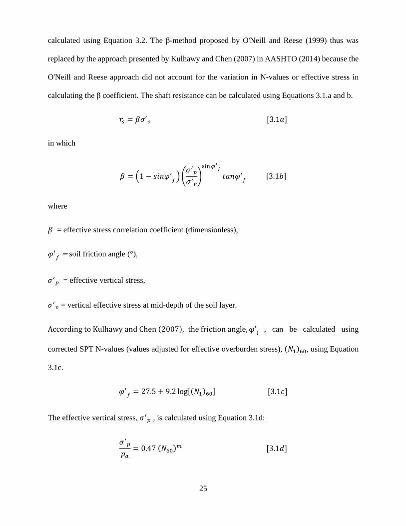
With regard to shaft resistance, Kulhawy and Chen (2007) proposed using the basic soil
parameter method by applying Equations 3.1a through 3.1d. Similarly, tip resistance can be
25
calculated using Equation 3.2. The β-method proposed by O'Neill and Reese (1999) thus was
replaced by the approach presented by Kulhawy and Chen (2007) in AASHTO (2014) because the
O'Neill and Reese approach did not account for the variation in N-values or effective stress in
calculating the β coefficient. The shaft resistance can be calculated using Equations 3.1.a and b.
Equation 4.4 implies that all the side resistance becomes negative and then is recovered by
half of the degraded side resistance in liquefiable layers. Higher values of �̅�𝑥 would result in lower
drag loads. The ultimate drag load corresponds to the case of �̅�𝑥 = 0, and �̅�𝑥 = 1 is the assumption
made in this study for analysis of the long-term after liquefaction cases. Appendix C justifies the
assumption of �̅�𝑥 = 1 for the unified method, showing that the unified method predicts the highest
values for drag load and downdrag settlement in case of �̅�𝑥 = 1. In the NP method, the liquefaction-
induced effects are reflected in both of load and resistance curves and considering the residual
strength would not lead to a more conservative analysis.
81
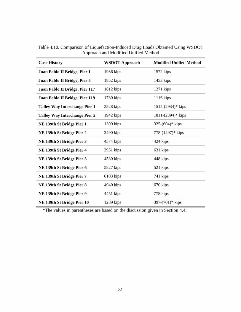
Table 4.10. Comparison of Liquefaction-Induced Drag Loads Obtained Using WSDOT Approach and Modified Unified Method
Case History WSDOT Approach Modified Unified Method
Juan Pablo II Bridge, Pier 1 1936 kips 1572 kips
Juan Pablo II Bridge, Pier 5 1852 kips 1453 kips
Juan Pablo II Bridge, Pier 117 1812 kips 1271 kips
Juan Pablo II Bridge, Pier 119 1730 kips 1116 kips
Talley Way Interchange Pier 1 2528 kips 1515-(2934)* kips
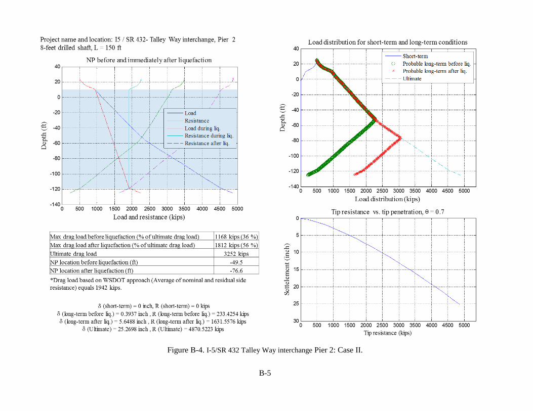
Talley Way Interchange Pier 2 1942 kips 1811-(2394)* kips
NE 139th St Bridge Pier 1 1309 kips 325-(604)* kips
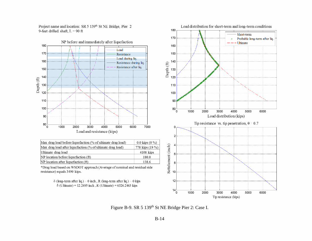
NE 139th St Bridge Pier 2 3490 kips 778-(1497)* kips
NE 139th St Bridge Pier 3 4374 kips 424 kips
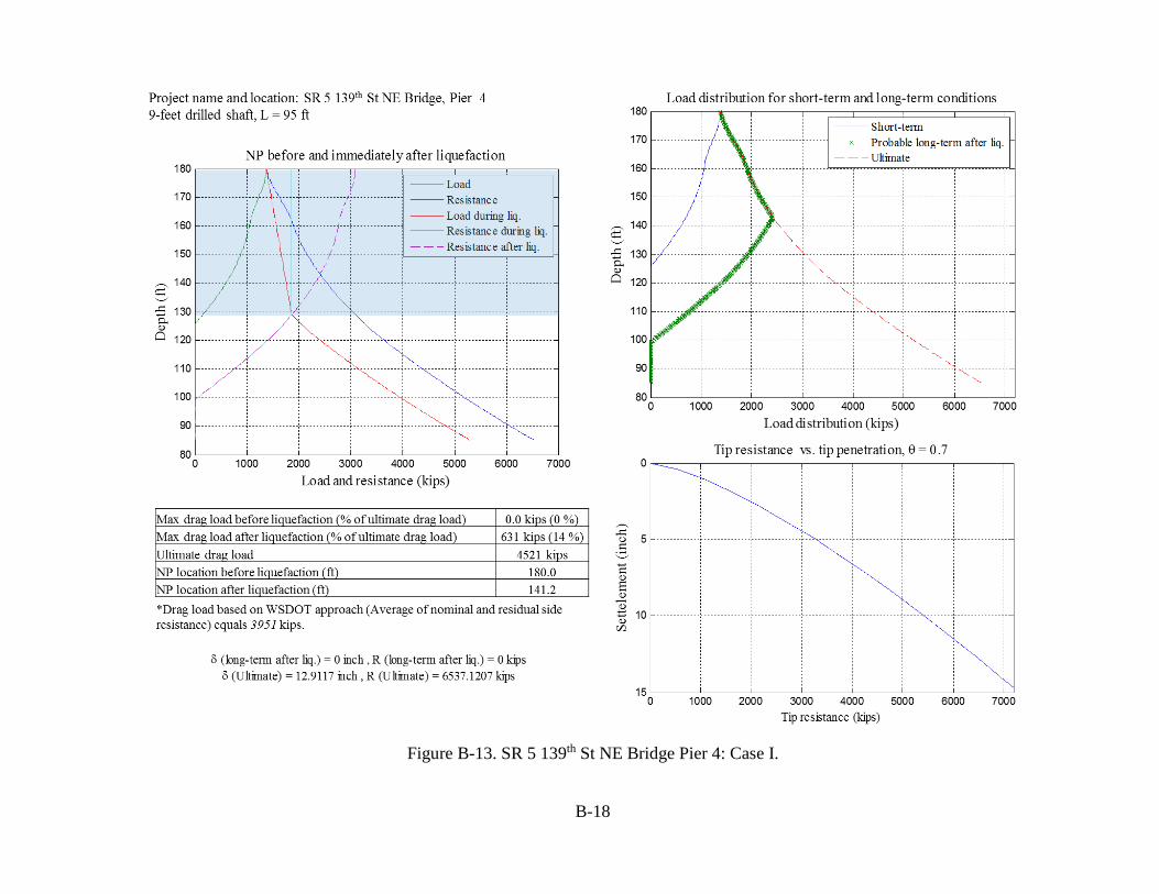
NE 139th St Bridge Pier 4 3951 kips 631 kips
NE 139th St Bridge Pier 5 4530 kips 448 kips
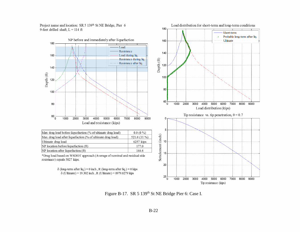
NE 139th St Bridge Pier 6 5827 kips 521 kips
NE 139th St Bridge Pier 7 6103 kips 741 kips
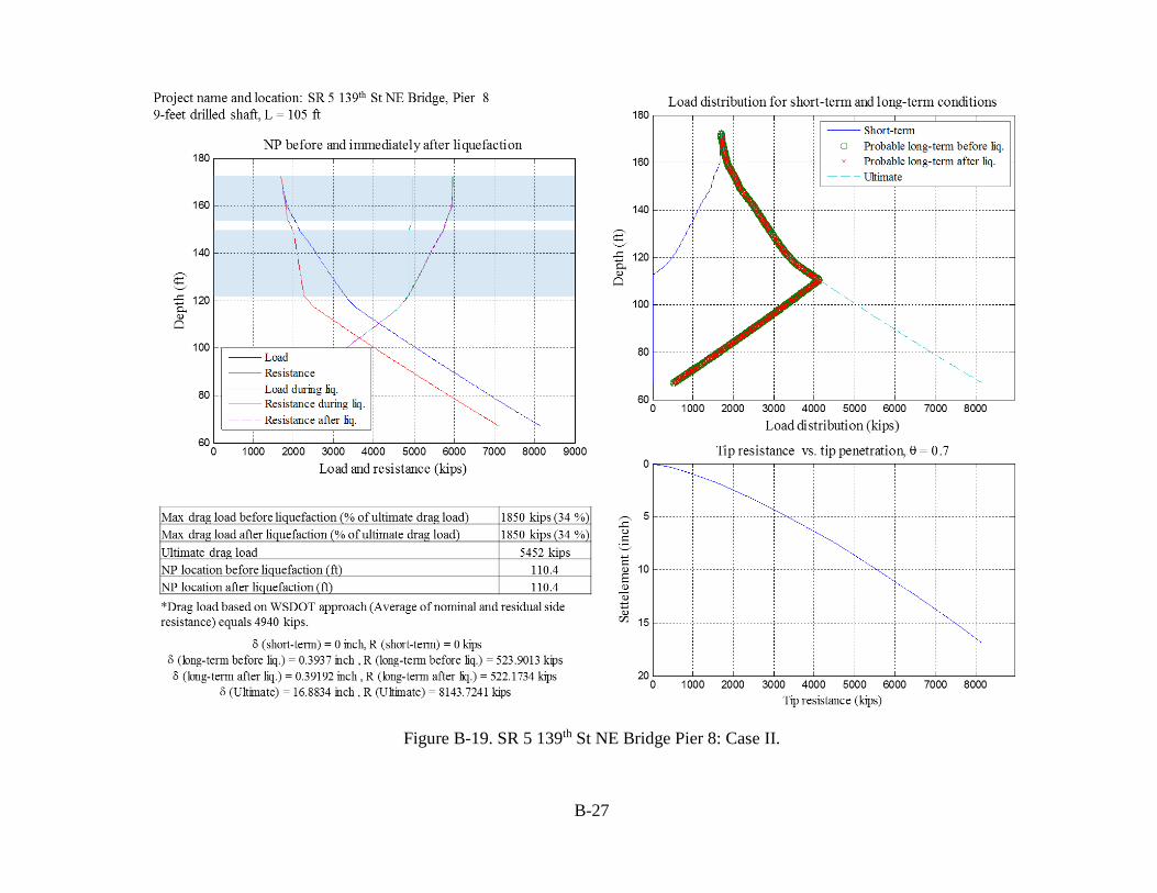
NE 139th St Bridge Pier 8 4940 kips 670 kips
NE 139th St Bridge Pier 9 4451 kips 778 kips
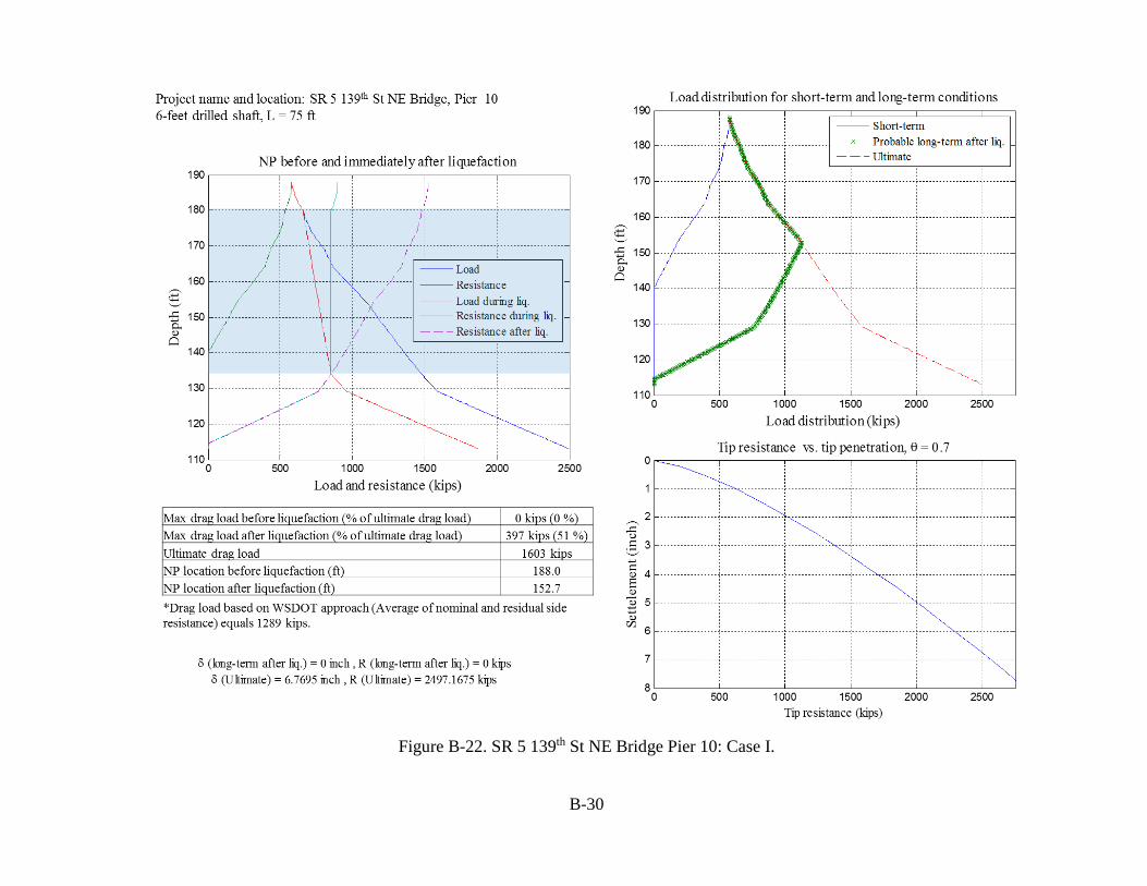
NE 139th St Bridge Pier 10 1289 kips 397-(701)* kips
*The values in parentheses are based on the discussion given in Section 4.4.
82
CHAPTER 5: CONCLUSIONS AND RECOMMENDATIONS
5.1. CONCLUSIONS
The downward relative movement of overlying soil layers around deep foundations induces
shear stress along drilled shafts and changes the axial load distribution on them. Depending on the
site conditions, the changes in the axial responses that result from liquefaction-induced settlement
can have a significant impact on the performance of drilled shafts and piles in seismic regions.
This study presents an analytical method to quantify the effects of liquefaction-induced downdrag
on piles and drilled shafts.
The analytical method is based on the NP method that was developed originally for clays
but has been modified to account for liquefaction-induced effects. This method assumes that the
soil settlement equals the pile settlement at the NP location and that the load transfer during
liquefaction within the liquefied layer during an earthquake is nearly zero. In this study, the NP
method was applied to an observed case of downdrag during the 8.8 magnitude earthquake in
Maule, Chile. The proposed unified method for drilled shafts was able to predict the downdrag
settlement observed at the site. Numerical simulations of the liquefaction-induced downdrag were
performed using OpenSees software to verify the key assumptions used in the analytical method.
The developed procedure also is illustrated for two field cases of drilled shafts in liquefiable soils
in Washington State.
Two different analysis methods are discussed in this report for comparative purposes (see
Section 3.3.1):
• Case I: No negative side resistance develops before liquefaction. This method is preferred
by AASHTO.
83
• Case II: Negative side resistance develops along the shaft. This study recommends 0.4 in.
downdrag settlement before liquefaction.
This study reached the following conclusions.
• The analysis results for a pier supporting the Juan Pablo II Bridge (Section 3.4) and for
both piers at the Talley Way interchange structure (Section 4.2) indicate that both Case I
and Case II analyses would result in practically the same downdrag settlements and drag
loads.
• The analysis results for the bridge piers at the NE 139th St. interchange (Section 4.3)
indicate that downdrag settlement was not significant at this site. However, the drag load
might be the controlling parameter in this case for liquefaction-induced downdrag analysis.
All the drag loads calculated using Case II analysis are larger than those calculated using
Case I analysis for this site. This finding indicates that Case II analysis is more conservative
in terms of drag loads calculated for shafts than Case I analysis.
• When a liquefiable layer is located below the shaft tip, the pile and soil systems above this
liquefiable layer will move together. In this case, the liquefaction-induced downdrag
settlement should be added to the settlement caused by compression of the liquefiable
zones below the shaft tip to find the total liquefaction-induced settlement. The drilled shafts
discussed in Chapter 3 for the Juan Pablo II Bridge are likely to experience such settlement
(see Section 3.4.3).
• Based on Case II analysis, the magnitude of the liquefaction-induced downdrag settlement
depends on the location of the liquefiable layers (above the NP, below the NP, and below
the pile tip).
o If a liquefiable layer is located above the NP, liquefaction-induced downdrag
settlements are negligible. In this case, however, very large drag loads could cause
84
structural failure of the shafts rather than settlement-induced failure of the structure.
All Case II analysis results for the drilled shafts in the NE 139th St. interchange,
except Piers 1, 2, and 10, are examples of this condition (see Appendix B).
o When a liquefiable layer is located below the NP, liquefaction-induced downdrag
effects occur as a result of changes to the NP location. The side resistance value of
the shaft during liquefaction will drop to zero momentarily throughout the
liquefiable layers. The lost positive side resistance (from layers below the NP)
transfers to the tip resistance, which causes downdrag settlement. After
liquefaction, with time, the drag load increases along with the development of
negative shaft resistance because of the relative settlement of the soil with respect
to the drilled shaft. The NP location after liquefaction would be lower than the case
before liquefaction that corresponds to higher values of negative side resistance or
drag load. All of the Case II analysis results for the drilled shafts at the Juan Pablo
II Bridge are examples of this condition (see Appendix B).
o If some layers are above the NP and some layers are below the NP, in order to have
a conservative liquefaction-induced downdrag design, the liquefiable layers above
the NP might not be considered liquefied during an earthquake (see Section 4.4).
• The need for using residual strength when pore pressure is not fully dissipated does not
arise when using the NP analysis (see Appendix C).
• The calculated drag loads on drilled shafts that are based on the modified unified method
are lower than the drag loads predicted using the current approach adopted by WSDOT
(see Section 4.5).
• If downdrag settlement before liquefaction is unlikely to happen, Case I analysis can be
performed with no further consideration. Although the results from the different case
85
studies reveal no significant difference in terms of downdrag settlement between Case I
and Case II analyses, the predicted drag loads are higher when using Case II analysis
compared to Case I analysis.
5.2. RECOMMENDATIONS
• This study focused on single piles, but most of the applications for pile foundations are for
pile groups. Extending this liquefaction-induced analysis for pile groups therefore is
recommended.
• This study’s approach assumes that tip resistance develops mainly after the side resistance
is fully mobilized to its capacity, and only the q-z function (tip resistance-vertical
movement of the shaft) is utilized. This assumption represents a simplified approach, but
it provides a very good estimation because the side resistance fully develops along the shaft
when only 10 percent of the tip resistance is mobilized (O'Neill and Reese 1999). Using
both the q-z and t-z functions (side resistance and vertical movement of the shaft) would
be more realistic to capture the load distribution along the shaft.
• This study considered liquefaction-induced downdrag, which is associated with earthquake
shaking. Pile movement involves not only vertical movement but also lateral movement.
This study recommends that p-y relationships that account for lateral movement should be
incorporated in future analysis. A complete model that accounts for vertical soil movement,
lateral soil movement, and inertial loads would give more insights about pile performance.
86
ACKNOWLEDGEMENTS
The authors would like to thank the Washington State Department of Transportation (WSDOT)
for its financial support of this research. We would also like to thank Dr. Bengt Fellenius for his
valuable remarks and guidance. Also, Tony Allen of WSDOT provided valuable comments and
input. Sincere thanks also are extended to Dr. Gonzalo Montalva at the University of Concepción,
Chile and Dr. Christian Ledezma Araya of the Pontificia Universidad Católica de Chile for
assisting in the collection and translation of relevant data.
87
REFERENCES
AASHTO (2014). LRFD Bridge Design Specifications. American Association of State Highway and Transportation Officials (4th ed.), Washington, DC.
Bjerrum, L. and I. J. Johannessen (1965). Measurements of the Compression of a Steel Pile to Rock Due to Settlement of the Surrounding Clay. Proceedings of the 6th International Conference on Soil Mechanics and Foundation Engineering, Montreal, Canada, September 8-15, University of Toronto Press, Vol. 2, 261-264.
Bjerrum, L., I. J. Johannessen, and O. Eide (1969). Reduction of Negative Skin Friction on Steel Piles to Rock. Proceedings of the 7th International Conference on Soil Mechanics and Foundation Engineering, Mexico City, Mexico, August 25-29, Mexico Geotechnical Society, Vol. 2, 27-34.
Boroschek, R. L., V. Contreras, D. Y. Kwak, and J. P. Stewart (2012). Strong Ground Motion Attributes of the 2010 M 8.8 Maule, Chile, Earthquake. Earthquake Spectra, S19-S38.
Boulanger, R. W. and S. J. Brandenberg (2004). Neutral Plane Solution for Liquefaction-Induced Down-Drag on Vertical Pile. (M. K. Yegian and E. Kavazanjian, eds.) Geotechnical Engineering for Transportation Projects, Proceedings of Geo-Trans 2004, Geotech, ASCE, Special Publication No. 126, 470-478.
Boulanger, R. W., B. L. Kutter, S. J. Brandenberg, et al. (2003). Pile Foundations in Liquefied and Laterally Spreading Ground during Earthquakes: Centrifuge Experiments and Analyses. Report No. UCD/CGM-03/01, Center for Geotechnical Modeling, Department of Civil Engineering, University of California, Davis, CA.
Bray, J. D. and J. D. Frost, eds. (2010). Geo-Engineering Reconnaissance of the 2010 Maule, Chile Earthquake. Report of the NSF-Sponsored GEER Association Team; primary authors: Arduino et al., <www.geerassociation.org>.
Canadian Geotechnical Society (1985). Canadian Foundation Engineering Manual (2nd ed.), Vancouver: BiTech Publishers,
Decourt, L. (1982). Prediction of Bearing Capacity of Piles Based Exclusively on N-values of the SPT. Proceedings of the ESOPT II, Amsterdam, 19-34.
Endo, M., A. Minou, T. Kawasaki, and T. Shibata (1969). Negative Skin Friction Acting on Steel Piles in Clay. Proceedings of the 8th International Conference on Soil Mechanics and Foundation Engineering, Mexico City, Mexico, August 25-29, Mexico Geotechnical Society, Vol. 2, 85-92.
Fellenius, B. H. and B. B. Broms (1969). Negative Skin Friction for Long Piles Driven in Clay. Proceedings of the 7th International Conference of Soil Mechanics and Foundation Engineering, Vol. 2, 93-98.
Fellenius, B. H. (1972). Downdrag on Long Piles in Clay Due to Negative Skin Friction. Canadian Geotechnical Journal, 9(4), 323-337.
Fellenius, B. H. (1984). Negative Skin Friction and Settlement of Piles. Proceedings of the 2nd International Seminar, Pile Foundations, Nanyang Technological Institute, Singapore,
88
Fellenius, B. H. (1988). Unified Design of Piles and Pile Groups Transportation Research Board Record, 1169, Transportation Research Board, Washington, DC, 75-82.
Fellenius, B. H. (1999). Bearing Capacity—A Delusion? Proceedings of the Annual Meeting of the Deep Foundation Institute, Hawthorne, NJ and Dearborn, MI, October 14-16,
Fellenius, B. H. (2004). Unified Design of Piled Foundations with Emphasis on Settlement Analysis. Honoring George G. Goble—Current Practice and Future Trends in Deep Foundations. Geo-Institute Geo TRANS Conference, Los Angeles, CA, July 27-30, 2004, edited by J. A. DiMaggio and M. H. Hussein. ASCE GSP 125, 253-275.
Fellenius, B. H. and T. C. Siegel (2008). Pile Design Consideration in a Liquefaction Event. Journal of Geotechnical and Environmental Engineering, ASCE, 132(9), 1412-1416.
Fellenius, B. H. (2014). Basics of Foundation Design. Electronic Ed., <www. Fellenius.net>.
Florin, V. A. and P. L. Ivanov (1961). Liquefaction of Saturated Sandy Soil. Proceedings of the 5th International Conference on Soil Mechanics and Foundation Engineering, Paris, France, 106.
Goudreault, P. A. and B. H. Fellenius. (2013). UniPile Version 5, Users and Examples Manual. UniSoft Geotechnical Solutions, Ltd. [www.UniSoftLtd.com],
Hanna, A. M. and A. Sharif (2006). Drag Force on Single Piles in Clay Subjected to Surcharge Loading. International Journal of Geomechanics, ASCE 6(2), 89-96.
Ishihara, K. and M. Yoshimine (1992). Evaluation of Settlements in Sand Deposits Following Liquefaction During Earthquakes. Soil Mechanics and Foundation Engineering 118(32), 173-188.
Jeong, S., J. Lee, and C. J. Lee. (2004). Slip Effect at the Pile-Soil Interface on Dragload. Computers and Geotechnics, 31, 115-126.
Johannessen, I. J. and L. Bjerrum (1965). Measurement of the Compression of a Steel Pile to Rock Due to Settlement of the Surrounding Clay. Proceedings of the 6th International Conference of Soil Mechanics and Foundation Engineering, Vol. 2, 261-264.
Knutson, L. and T. C. Siegel (2006). Consideration of Drilled Displacement Piles for Liquefaction Mitigation. Proceedings of DFI Augered Cast-in-Place Pile Committee Specialty Seminar, 129-132.
Kramer, S. L. (1996). Geotechnical Earthquake Engineering. Upper Saddle River, NJ: Prentice Hall.
Ledezma, C., T. Hutchinson, S. A. Ashford, et al. (2012). Effects of Ground Failure on Bridges, Roads, and Railroads. Earthquake Spectra 28(S1), S119-S143.
Lee, C. J. and W. W. Ng (2004). Development of Down-drag on Piles and Pile Groups in Consolidating Soil. Journal of Geotechnical and Geoenvironmental Engineering, ASCE, 130(9), 905-914.
Lee, K. L. and A. Albeisa (1974). Earthquake Induced Settlements in Saturated Sands. Journal of the Soil Mechanics and Foundation Division, ASCE, Vol. 100, No. GT4, April.
Lu, J., A. Elgamal, and Z. Yang (2011). OpenSeesPL: 3D Lateral Pile-Ground Interaction. User Manual (Beta 1.0). University of California, San Diego, CA.
89
Lysmer, J. and A. M. Kuhlemeyer (1969). Finite Dynamic Model for Infinite Media. Journal of the Engineering Mechanics Division, ASCE, 95, 859-877.
Matyas, E. L. and J. C. Santamarina (1994). Negative Skin Friction and the Neutral Plane. Canadian Geotechnical Journal 31(3), 591-597.
Meyerhof, G. G. (1976). Bearing Capacity and Settlement of Pile Foundations. The Eleventh Terzaghi Lecture, November 5, 1975. Journal of Geotechnical Engineering, ASCE, 102(GT3) 195-228.
O'Neill, M. W. and L. C. Reese (1999). Drilled Shafts. Construction Procedures and Design Methods. Federal Highway Administration, Report No. FHWA-IF99-025, Transportation Research Board, Washington, DC.
OpenSees (2014). Open System for Earthquake Engineering Simulation. Pacific Earthquake Engineering Research Center (PEER), University of California, Berkeley, CA. http://opensees.berkeley.edu.
Parra, E. (1996). Numerical Modeling of Liquefaction and Lateral Ground Deformation Including Cyclic Mobility and Dilation Response in Soil Systems. Ph.D. dissertation, Rensselaer Polytechnictechnic Institute, New York, NY.
Poulos, H. and E. H. Davis (1990). Pile Foundation Analysis and Design (reprint ed.). Robert E. Krieger Publishing Company, FL.
Prevost, J. H. (1985). A Simple Plasticity Theory for Frictional Cohesionless Soils. Soil Dynamics and Earthquake Engineering 4(1), 9-17.
Rollins, K. M. and S. R. Strand (2006). Downdrag Forces Due to Liquefaction Surrounding a Pile. Proceedings of the 8th U.S. National Conference on Earthquake Engineering. Paper No. 1646, San Francisco, CA, April 18-22.
Seed, H. B. et al. (1975). The Generation and Dissipation of Pore Water Pressures During Soil Liquefaction. Report No. UCB/EERC-75/26, University of California, Berkeley, CA.
Siegel, T. C. et al. (2014). Neutral Plane Method for Drag Force of Deep Foundations and the AASHTO LRFD Bridge Design Specifications.
Strand, S. R. (2008). Liquefaction Mitigation Using Vertical Composite Drains and Liquefaction-induced Downdrag on Piles: Implications for Deep Foundation Design. Ph.D. thesis, Department of Civil and Environmental Engineering, Brigham Young University, Provo, UT.
Tokimatsu, K. and H. B. Seed (1987) Evaluation of Settlements in Sands Due to Earthquake Shaking. Journal of Geotechnical Engineering, ASCE, 113(8), 861-879.
United States Geological Survey (USGS) (2012). USGS Earthquake Hazards Program, Chile Earthquake of 27 Feb 2010. http://www.strongmotioncenter.org/cgi-bin/CESMD/iqr_dist_DM2.pl?IQRID=Chile_27Feb2010_us2010tfan&SFlag=0&Flag=2. (last accessed 17 March 2014).
Verdugo, R. and G. Peters (2010). Informe Geotécnico Fase Anteproyecto Infraestructura Puente. Mecano Eje Chacabuco, Rev7, August.
90
Wang, R. and S. J. Brandenberg (2013). Beam on Nonlinear Winkler Foundation and Modified Neutral Plane Solution for Calculating Downdrag Settlement. Journal of Geotechnical and Geoenvironmental Engineering, ASCE, doi:10.1061/(ASCE)GT.1943-5606.0000888.
Washington State Department of Transportation (WSDOT) (2013). Geotechnical Design Manual M 46-03.09. < http://www.wsdot.wa.gov/publications/manuals/m46-03.htm>.
Yan, W. M., T. K. Sun, and L. G. Tham (2012). Coupled-Consolidation Modeling of a Pile in Consolidating Ground. Journal of Geotechnical and Geoenvironmental Engineering, ASCE, 138(7) 789-798.
Yen, W. P., G. Chen, I. Buckle, et al. (2011). Post-Earthquake Reconnaissance Report on Transportation Infrastructure: Impact of the February 27, 2010, Offshore Maule Earthquake in Chile. Federal Highway Administration, Report No. FWWA-HRT-11-030, 214.
Yang, Z. (2000). Numerical Modeling of Earthquake Site Response Including Dilation and Liquefaction. Ph.D. dissertation, Columbia University, New York, NY.
Yang, Z. and A. Elgamal (2002). Influence of Permeability on Liquefaction-Induced Shear Deformation. Journal of Engineering Mechanics, ASCE, 128(7), 720-729.
Yang, Z., A. Elgamal, and J. Parra (2003). Computational Model for Cyclic Mobility and Associated Shear Deformation. Journal of Geotechnical and Geoenvironmental Engineering, ASCE, 129(12), 1119-1127.
Yang, Z. and A. Elgamal (2008). OpenSees Soil Models and Solid-Fluid Fully Coupled Elements. User’s Manual, 2008 (Version 1.0). University of California, San Diego, CA.
Youd, T. L., I. M. Idriss, R. D. Andrus, et al. (2001). Liquefaction Resistance of Soils: Summary Report from the 1996 NCEER and 1998 NCEER/NSF Workshop on Evaluation of Liquefaction Resistance of Soils. Journal of Geotechnical and Geoenvironmental Engineering, ASCE, 127(10), 817-833.
A-1
APPENDIX A: NUMERICAL ANALYSIS OF STRESS AND SETTLEMENT SOIL RESPONSES
A.1 INTRODUCTION
The neutral plane (NP) analysis presented in Chapter 3 makes the assumption that the pile
settlement equals the soil settlement at the equilibrium location and that the load transfer during
liquefaction within the liquefied layer is nearly zero. This assumption is in contrast with that of
Wang and Brandenberg (2013) who assume that the relative velocity between the pile and the soil
is zero at the NP location. In order to examine the validity of the assumptions for liquefaction, a
numerical simulation of the downdrag problem was conducted for this study using finite element
analysis.
OpenSees (Open System for Earthquake Engineering Simulation) is a widely used finite
element software package in earthquake geotechnical engineering that has been made available as
an open source for users. Many solution procedures and algorithms are available in OpenSees to
solve linear and nonlinear structural and geotechnical problems under static or dynamic loading.
OpenSees uses a fully programmable scripting language, tcl (tool command language), to define
models, analysis steps, and output results (OpenSees 2014). OpenSees often is used by
geotechnical engineers to predict ground surface motions in order to develop design response
spectra, evaluate dynamic stresses and strains of liquefaction hazards, and determine earthquake-
induced forces (Kramer 1996). However, this study focused on the use of numerical analysis to
predict stress and settlement responses in order to verify the downdrag analysis method developed
in Chapter 3. A soil profile was idealized using a two-dimensional single column in OpenSees,
and then the profile was subjected to ground motion.
A-2
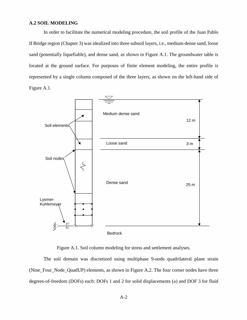
A.2 SOIL MODELING
In order to facilitate the numerical modeling procedure, the soil profile of the Juan Pablo
II Bridge region (Chapter 3) was idealized into three subsoil layers, i.e., medium-dense sand, loose
sand (potentially liquefiable), and dense sand, as shown in Figure A.1. The groundwater table is
located at the ground surface. For purposes of finite element modeling, the entire profile is
represented by a single column composed of the three layers, as shown on the left-hand side of
Figure A.1.
Figure A.1. Soil column modeling for stress and settlement analyses.
The soil domain was discretized using multiphase 9-node quadrilateral plane strain
(Nine_Four_Node_QuadUP) elements, as shown in Figure A.2. The four corner nodes have three
degrees-of-freedom (DOFs) each: DOFs 1 and 2 for solid displacements (u) and DOF 3 for fluid
Bedrock
Dense sand
Loose sand
Medium dense sand
3 m
25 m
12 m
Lysmer-Kuhlemeyer
Soil elements
Soil nodes
A-3
pressure (p). The other five nodes have two DOFs each for solid displacements. This element is
based on Biot’s theory of a porous medium that captures the dynamic response of solid-fluid fully
coupled material (Yang and Elgamal 2008). The soil profile was discretized into 0.2-m elements
Figure B-7. SR 5 139th St NE Bridge Pier 1: Case I.
B-13
Figure B-8. SR 5 139th St NE Bridge Pier 1: Case II.
B-14
Figure B-9. SR 5 139th St NE Bridge Pier 2: Case I.
B-15
Figure B-10. SR 5 139th St NE Bridge Pier 2: Case II.
B-16
Figure B-11. SR 5 139th St NE Bridge Pier 3: Case I.
B-17
Figure B-12. SR 5 139th St NE Bridge Pier 3: Case II.
B-18
Figure B-13. SR 5 139th St NE Bridge Pier 4: Case I.
B-19
Figure B-14. SR 5 139th St NE Bridge Pier 4: Case II.
B-20
Figure B-15. SR 5 139th St NE Bridge Pier 5: Case I.
B-21
Figure B-16. SR 5 139th St NE Bridge Pier 5: Case II.
B-22
Figure B-17. SR 5 139th St NE Bridge Pier 6: Case I.
B-23
Figure B-15. SR 5 139th St NE Bridge Pier 6: Case II.
B-24
Figure B-16. SR 5 139th St NE Bridge Pier 7: Case I.
B-25
Figure B-17. SR 5 139th St NE Bridge Pier 7: Case II.
B-26
Figure B-18. SR 5 139th St NE Bridge Pier 8: Case I.
B-27
Figure B-19. SR 5 139th St NE Bridge Pier 8: Case II.
B-28
Figure B-20. SR 5 139th St NE Bridge Pier 9: Case I.
B-29
Figure B-21. SR 5 139th St NE Bridge Pier 9: Case II.
B-30
Figure B-22. SR 5 139th St NE Bridge Pier 10: Case I.
B-31
Figure B-23. SR 5 139th St NE Bridge Pier 10: Case II.
B-32
Figure B-24. Juan Pablo II Bridge Piers 1 and 2: Case I.
B-33
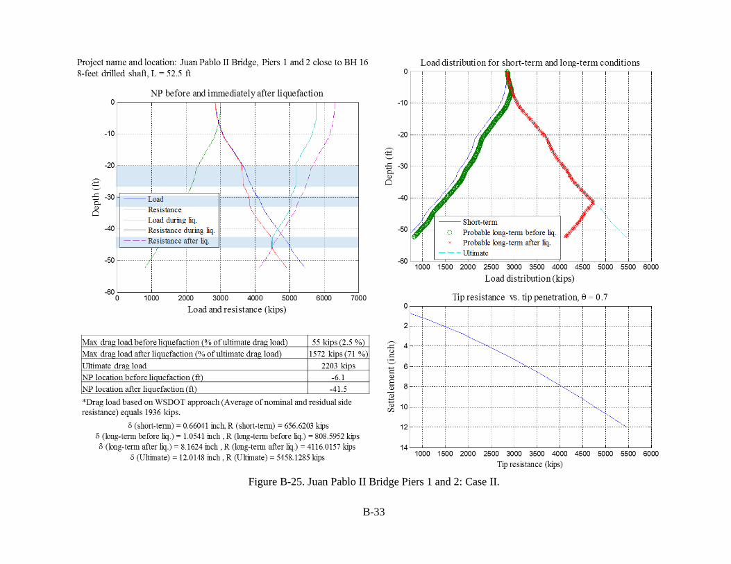
Figure B-25. Juan Pablo II Bridge Piers 1 and 2: Case II.
B-34
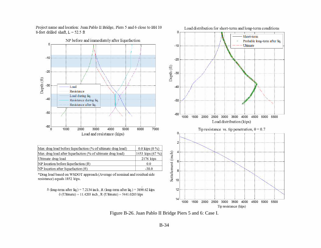
Figure B-26. Juan Pablo II Bridge Piers 5 and 6: Case I.
B-35
Figure B-27. Juan Pablo II Bridge Piers 5 and 6: Case II.
B-36
Figure B-28. Juan Pablo II Bridge Piers 117 and 118: Case I.
B-37
Figure B-29. Juan Pablo II Bridge Piers 117 and 118: Case II.
B-38
Figure B-30. Juan Pablo II Bridge Piers 119 and 120: Case I.
B-39
Figure B-31. Juan Pablo II Bridge Piers 119 and 120: Case II.
C-1
APPENDIX C: NEUTRAL PLANE METHOD AND THE POSSIBLE NEED TO USE RESIDUAL STRENGTH IN LIQUEFIED LAYERS
The American Association of State Highway and Transportation Officials (AASHTO)
(2014) recommends the use of residual strength in liquefiable layers for the explicit method of
design, as discussed in Chapter 2. Here we discusses the possible need for implications regarding
the use of residual strength on neutral plane (NP) method.
The side resistance of a drilled shaft is a function of the excess pore water pressure ratio, ru,
as shown in fs = σvo′ Ko tan(δ)(1− ru) (Boulanger and Brandenberg 2004). At the moment of
initial liquefaction ru equals 1; this value will gradually decrease to zero as the excess pore water
pressure dissipates. The corresponding effect on the shaft will be dependent on the location of the
liquefiable layer with respect to the NP.
Figure C.1 presents the variations in the load and resistance curves for the case when ru = 1
(Line 1), during pore pressure dissipation (Line 2), and after complete dissipation (Line 3) for the
case when the liquefiable layer is above the NP. Note that the dashed lines represent the load and
the solid lines represent resistance. Because tip resistance will not be affected when the liquefiable
layer is above the NP, no change in settlement will occur at any time. However, the drag load would
decrease during seismic action and as the excess pore pressure increases to ru = 1. Also, the drag
load would revert to the static condition, as shown schematically in Figure C1 (a). So, the maximum
drag load would remain the same as it is in the static condition.
C-2
Figure C.2 presents the variations in the load and resistance curves for the case when ru = 1
(Line 1), during pore pressure dissipation (Line 2), and after complete dissipation (Line 3) for the
case when the liquefiable layer is below the NP. As in Figure C1, the dashed lines represent the
load and the solid lines represent resistance. The tip resistance for this case will increase during
seismic action until ru = 1, but will remain constant at this value during excess pore pressure
dissipation and even after complete dissipation. The downdrag settlement would correspond to the
increased tip resistance. For this case, the drag load would increase and reach its maximum value
when ru = 0.
Clearly, this discussion suggests that the need for residual strength does not arise when the
pore pressure is not fully dissipated when using NP analysis. The most critical condition for
liquefaction-induced drag load and downdrag settlement on deep foundations is when the excess
pore pressure has fully dissipated.
The same discussion holds if the side resistance of shaft decrease because of the
liquefaction-induced effects and changes the soil properties after fully dissipation of pore water
pressure. In the NP method, the liquefaction-induced effects are reflected in both of load and
resistance curves and considering the residual strength would not lead to a more conservative
analysis.
C-3
Figure C.1. Comparison of drag loads (DLs) during and after liquefaction when the liquefiable
layer is above the neutral plane (NP).
C-4
Figure C.2. Comparison of drag loads (DLs) during and after liquefaction when the liquefiable
layer is below the neutral plane (NP).
Americans with Disabilities Act (ADA) Information: This material can be made available in an alternate format by emailing the Office of Equal Opportunity at [email protected] or by calling toll free, 855-362-4ADA(4232). Persons who are deaf or hard of hearing may make a request by calling the Washington State Relay at 711.
Title VI Statement to Public: It is the Washington State Department of Transportation’s (WSDOT) policy to assure that no person shall, on the grounds of race, color, national origin or sex, as provided by Title VI of the Civil Rights Act of 1964, be excluded from participation in, be denied the benefits of, or be otherwise discriminated against under any of its federally funded programs and activities. Any person who believes his/her Title VI protection has been violated, may file a complaint with WSDOT’s Office of Equal Opportunity (OEO). For additional information regarding Title VI complaint procedures and/or information regarding our non-discrimination obligations, please contact OEO’s Title VI Coordinator at (360) 705-7082.