16
•

Loughborough UniversityInstitutional Repository
Liquid drops on a surface:using density functionaltheory to calculate the
binding potential and dropprofiles and comparing withresults from mesoscopic
modelling
This item was submitted to Loughborough University's Institutional Repositoryby the/an author.
Citation: HUGHES, A.P., THIELE, U. and ARCHER, A.J., 2015. Liquiddrops on a surface: using density functional theory to calculate the binding po-tential and drop profiles and comparing with results from mesoscopic modelling.Journal of Chemical Physics, 142 (7), 074702.
Additional Information:
• Copyright 2014 American Institute of Physics. This article may be down-loaded for personal use only. Any other use requires prior permission ofthe author and the American Institute of Physics. The following articleappeared in Journal of Chemical Physics, 142 (7), 074702 and may befound at: http://dx.doi.org/10.1063/1.4907732
Metadata Record: https://dspace.lboro.ac.uk/2134/16889
Version: Published
Publisher: c© AIP Publishing LLC
Please cite the published version.
Liquid drops on a surface: Using density functional theory to calculate the bindingpotential and drop profiles and comparing with results from mesoscopic modellingAdam P. Hughes, Uwe Thiele, and Andrew J. Archer Citation: The Journal of Chemical Physics 142, 074702 (2015); doi: 10.1063/1.4907732 View online: http://dx.doi.org/10.1063/1.4907732 View Table of Contents: http://scitation.aip.org/content/aip/journal/jcp/142/7?ver=pdfcov Published by the AIP Publishing Articles you may be interested in An introduction to inhomogeneous liquids, density functional theory, and the wetting transition Am. J. Phys. 82, 1119 (2014); 10.1119/1.4890823 Understanding wetting of immiscible liquids near a solid surface using molecular simulation J. Chem. Phys. 139, 064110 (2013); 10.1063/1.4817535 Spectral methods for the equations of classical density-functional theory: Relaxation dynamics of microscopicfilms J. Chem. Phys. 136, 124113 (2012); 10.1063/1.3697471 Monte Carlo simulation strategies for computing the wetting properties of fluids at geometrically roughsurfaces J. Chem. Phys. 135, 184702 (2011); 10.1063/1.3655817 Nanodrop on a nanorough solid surface: Density functional theory considerations J. Chem. Phys. 129, 014708 (2008); 10.1063/1.2951453
This article is copyrighted as indicated in the article. Reuse of AIP content is subject to the terms at: http://scitation.aip.org/termsconditions. Downloaded to IP:
128.176.202.20 On: Tue, 17 Feb 2015 16:27:27

THE JOURNAL OF CHEMICAL PHYSICS 142, 074702 (2015)
Liquid drops on a surface: Using density functional theory to calculatethe binding potential and drop profiles and comparing with resultsfrom mesoscopic modelling
Adam P. Hughes,1,a) Uwe Thiele,2,3,4,b) and Andrew J. Archer1,c)1Department of Mathematical Sciences, Loughborough University, Loughborough LE11 3TU, United Kingdom2Westfälische Wilhelms-Universität Münster, Institut für Theorestische Physik, Wilhelm-Klemm-Str. 9,48149 Münster, Germany3Center of Nonlinear Science (CeNoS), Westfälische Wilhelms Universität Münster, Corrensstr. 2,48149 Münster, Germany4Center for Multiscale Theory and Computation (CMTC), University of Münster, Corrensstr. 40, 48149Münster, Germany
(Received 13 October 2014; accepted 27 January 2015; published online 17 February 2015)
The contribution to the free energy for a film of liquid of thickness h on a solid surface due tothe interactions between the solid-liquid and liquid-gas interfaces is given by the binding potential,g(h). The precise form of g(h) determines whether or not the liquid wets the surface. Note thatdifferentiating g(h) gives the Derjaguin or disjoining pressure. We develop a microscopic densityfunctional theory (DFT) based method for calculating g(h), allowing us to relate the form of g(h)to the nature of the molecular interactions in the system. We present results based on using a simplelattice gas model, to demonstrate the procedure. In order to describe the static and dynamic behaviourof non-uniform liquid films and drops on surfaces, a mesoscopic free energy based on g(h) is oftenused. We calculate such equilibrium film height profiles and also directly calculate using DFT thecorresponding density profiles for liquid drops on surfaces. Comparing quantities such as the contactangle and also the shape of the drops, we find good agreement between the two methods. Wealso study in detail the effect on g(h) of truncating the range of the dispersion forces, both thosebetween the fluid molecules and those between the fluid and wall. We find that truncating can havea significant effect on g(h) and the associated wetting behaviour of the fluid. C 2015 AIP PublishingLLC. [http://dx.doi.org/10.1063/1.4907732]
I. INTRODUCTION
The wetting of a substrate by a fluid is an important phys-ical process and understanding such behaviour is crucial in avariety of fields from industrial processes such as lubricationand painting to biological applications such as tear films in theeyes or mucus linings in the lungs. The wetting behaviour ofa fluid1,2 is determined by the manner in which the atoms ormolecules within the fluid interact with each other and withthose forming the substrate. Determining the macroscopic fluidproperties, wetting behaviour and thermodynamics, startingfrom an understanding of the (microscopic) molecular interac-tions is one of the cornerstone problems in liquid state science.2
On the macroscopic scale, the wetting behaviour of a fluidin contact with a solid substrate can be characterised by thecontact angle that a liquid drop makes with that substrate.Three regimes of wetting behaviour can be identified: completewetting, partial wetting, and non-wetting, these three statesare defined by contact angles of θ = 0, 0 < θ < 180, and θ= 180, respectively.1 Surface tension forces arise from inter-faces in the fluid and these can be related to the contact angleby Young’s equation2
a)Electronic address: [email protected])Electronic address: [email protected])Electronic address: [email protected]
cos θ =γwg − γwl
γlg, (1)
where γlg, γwl, and γwg are the liquid-gas, wall-liquid, and wall-gas surface tensions, respectively.
The effective interface Hamiltonian (IH) model,3–6 alsoreferred to as the interface free energy model, describes theheight profile of a mesoscopic liquid film on a substrate. Onecan find the equilibrium shape of a droplet by minimising thefree energy functional
F[h] =
g(h) + γlg
1 + (∇h)2
dx, (2)
where h(x) is the liquid film thickness at some point x onthe substrate and g(h) is the binding potential, which is alsoreferred to as the effective interface potential.3–8 g(h) is arestricted free energy, i.e., the free energy subject to the con-straint that the thickness of the liquid layer adsorbed on thesurfaces is h. A good discussion on the subject of restricted freeenergies can be found in Ref. 9. The binding potential describesthe interaction between two interfaces and is related to thedisjoining pressureΠ = −∂g/∂h. In the IH model, the bindingpotential is often approximated by simple expressions thatgive the qualitatively correct behaviour. A common exampleof such an approximation would be an asymptotic expansionwhich is valid only for larger film thicknesses (cf. Sec. II). This
0021-9606/2015/142(7)/074702/14/$30.00 142, 074702-1 © 2015 AIP Publishing LLC
This article is copyrighted as indicated in the article. Reuse of AIP content is subject to the terms at: http://scitation.aip.org/termsconditions. Downloaded to IP:
128.176.202.20 On: Tue, 17 Feb 2015 16:27:27

074702-2 Hughes, Thiele, and Archer J. Chem. Phys. 142, 074702 (2015)
paper sets out a method to directly calculate the binding poten-tial from a microscopic basis, namely, via density functionaltheory (DFT).2,10–15 As input, the method takes the interactionsbetween particles in the fluid and also the forces on the fluidparticles due to any external fields, for example, that due to thewall of a container or a surface on which the liquid is deposited.This calculation yields an expression for the binding potentialthat is valid for all film thicknesses. The term “particle” is usedhere generically to refer to the atoms/molecules/colloids in thefluid, depending on the exact system under study. Note that itis also possible to calculate g(h) from computer simulations—see Refs. 16–23.
The IH model is particularly useful due to its application indynamical studies. By making the assumption of small surfacegradients and contact angles, Eq. (2) reduces to
F[h] =
g(h) + γlg
2(∇h)2
dx, (3)
where we have omitted a constant contribution. Equation (3)can then be employed in the thin film (or long-wave) evolutionequation,24,25 which describes the time evolution of a thin filmof liquid on a flat solid substrate. In gradient dynamics form,it is written26,27
∂h∂t= ∇ ·
Q(h)∇ δF[h]
δh
, (4)
where Q(h) is a mobility factor that depends on the film thick-ness h(x, t). Equation (4) may be derived by making a longwave approximation in the governing Navier-Stokes equa-tion.25,28 There are many applications of this equation to modeldifferent situations. Steady state solutions, where ∂h/∂t = 0,such as drop profiles, are found by minimising the free energy,Eq. (3), with respect to the film height profile, subject to avolume constraint. More specifically, it amounts to solving
δFδh= α, (5)
where α is a Lagrange multiplier stemming from the constrainth(x) dx = V0, (6)
where V0 is a specified drop volume. A typical drop profileresulting from such a calculation can be seen in Fig. 1(a). Notethe very thin non-zero height “precursor” film that is presentto the left and right of the drop.
A fully microscopic description has statistical mechanicsas its basis. Statistical mechanics calculates an average over anensemble of all possible states of the system, i.e., it averagesover all possible configurations of the particles. This averageleads to determining the fluid one body density profile ρ(r),which represents the likelihood of finding a particle at a givenpoint r in the system.2 This statistical mechanical point of viewis the basis for DFT. From DFT, the grand potential, Ω, ofthe system is calculated and the equilibrium density profile,ρ(r), which minimises Ω, can be found. A typical equilibriumdensity profile of a liquid drop on a solid substrate is displayedin Fig. 1(b). Other examples of drop profiles calculated usingDFT can be found in Refs. 29–33. Note that by identifyingthe surface of the liquid as the surface where the densityequals a specified value, ρint, where ρl > ρint > ρg and where
FIG. 1. Two different descriptions of a liquid drop on a surface: (a) a heightprofile calculated via Eq. (7) from a mesoscopic free energy (cf. Eq. (2)) and(b) a density profile, which gives the fluid number density at a distance zabove the surface. These are both for a fluid with βϵ = 0.9 and βϵw = 0.6(see Sec. III for further details).
ρl and ρg are the coexisting liquid and gas densities of thefluid, the description can be further reduced to obtain a filmheight profile very similar to that displayed in Fig. 1(a). Onepossible choice is to choose ρint = (ρl + ρg)/2. Alternatively,by integrating in the z direction over such a density profile, wecan obtain a drop height profile. Here, we define the height ofthe liquid film on a substrate as the adsorption divided by theliquid-gas bulk density difference
h(x, y) = ∞
0
ρ(x, y, z) − ρg
dz
ρl − ρg. (7)
It is worth noting that using DFT it is just as easy to computethe profile for a liquid droplet that makes a contact angle withthe substrate that is greater than 90, than one with θ < 90. Itis significantly more difficult to find drop profiles for θ > 90
in the mesoscopic approach because for these contact angles,Eqs. (2) and (3) cannot be employed.
The remainder of this paper is set out as follows: in Sec. II,the binding potential and the procedure for calculating it arediscussed. A simple DFT, for the lattice-gas model, is pre-sented in Sec. III that is used to demonstrate the procedure. Thedependence of the fluid behaviour on the particle interactionsis discussed in Sec. IV. In particular, it is shown that truncatingthe range of the dispersion interactions between the particleshas a profound effect on the binding potential and interfacialphase behaviour. The method of fitting a function to the calcu-lated data is given in Sec. V, followed by the results of passingthe binding potential from the lattice-gas model to the thin filmIH model in Sec. VI. Finally, conclusions are drawn in Sec. VII.
II. THE BINDING POTENTIAL
For any fluid, coexistence between the liquid and gasphases occurs when the temperature T , chemical potential µ,and pressure p of the two phases are equal. It then follows, fora given volume V , that the bulk grand free energy, Ω = −pV ,of either phase occupying the same volume is also equal. For asystem where the liquid and gas phases of a fluid exist together
This article is copyrighted as indicated in the article. Reuse of AIP content is subject to the terms at: http://scitation.aip.org/termsconditions. Downloaded to IP:
128.176.202.20 On: Tue, 17 Feb 2015 16:27:27

074702-3 Hughes, Thiele, and Archer J. Chem. Phys. 142, 074702 (2015)
at the point of liquid-gas coexistence, any excess, over bulk,contributions to the free energy of the system must stem solelyfrom the interface that forms between the two phases. Thisexcess grand potential per unit area of the interface defines thesurface tension between those two phases. In this case, it isthe liquid-gas surface tension γlg. Now, consider a system withchemical potential µ = µcoex, the value at coexistence, where afilm of liquid separates the bulk gas from a solid surface (cf.Fig. 2). The excess free energy now consists of the sum of thetwo interfacial tensions and also the interaction between thetwo interfaces. The excess grand potential in such a system isgiven by Ωex(h) ≡ Ω + pV = ωex(h)A, where A is the area ofthe interface and
ωex(h) = γwl + γlg + g(h), (8)
h is the liquid film thickness, γwl and γlg are the wall-liquidand liquid-gas surface tensions, respectively.34 The final termg(h) is the binding potential, which gives the contribution tothe free energy from the interaction between the two interfaces.This has the property that as h → ∞, g(h) → 0. The absoluteminimum of the grand potential defines the equilibrium filmthickness h.
In the case of liquid droplets surrounded by their vapouron a solid substrate, the absolute minimum of the bindingpotential is directly related to the equilibrium contact angle ofthe drop,35,36
θ = cos−1(1 +
g(h0)γlg
), (9)
where g(h0) is the value at the minimum of the binding poten-tial. This corresponds directly to Young’s equation, Eq. (1);the absolute minimum of the binding potential corresponds tothe equilibrium state of the system and gives the equilibriumexcess grand potential, i.e., the wall-gas surface tension
ω(h0) = γwl + γlg + g(h0) = γwg. (10)
Replacing γwg in Eq. (1) with this expression leads to Eq. (9).Equation (8) is given above as a function of the film height
h. From a microscopic viewpoint, it is often more convenientto use the adsorption of the fluid as the order parameter charac-terising the fluid at the interface, instead of the film thickness.The total adsorption is readily calculated from the fluid densityprofile as
Γ =1A
(ρ(r) − ρb) dr. (11)
FIG. 2. A schematic of the system: a film of liquid of thickness h separatinga semi-infinite volume of gas from a solid surface.
ρb is the equilibrium bulk fluid density, which in the casesconsidered here is the gas density ρg . We may also define alocal adsorption [c.f. Eq. (7)] as follows:
Γ(x, y) = ∞
0
ρ(x, y, z) − ρg
dz, (12)
so that when the definition in Eq. (7) for the film height h isused, we have Γ = h(ρl − ρg). For other definitions of the filmheight h, then
Γ ≈ h(ρl − ρg). (13)
The dependence on how precisely h is defined becomes negli-gible, for large h. Thus, Eq. (8) and also the binding potentialg may be given as a function of the adsorption. Note, however,that negative adsorptions are possible, e.g., at a purely repulsivewall, and in such a situation, describing the liquid film at thewall via a film thickness h becomes meaningless, since thequantity h defined in Eq. (7) then becomes negative.
For a system with chemical potential µ = µcoex − δµ,i.e., off-coexistence, then there is an additional contributionΓδµ, that must be added to the right hand side of Eq. (8).4,37
Together with Eq. (13), this gives
ωex(h) ≈ γwl + γlg + (ρl − ρg)hδµ + g(h). (14)
Often, asymptotic forms of binding potentials are usedwhich are strictly valid only in the limit of a large film thick-ness.4 There are two main asymptotic forms of the bindingpotential that are considered, the choice of which dependson the assumed particle interactions and the range of thoseinteractions. For van der Waals’ (dispersion) interactions, thefollowing asymptotic form is appropriate:3,38–40
g(h) = ah2 +
bh3 + · · ·. (15)
The equivalent disjoining pressure is24,25
Π(h) = 2ah3 +
3bh4 + · · ·. (16)
Under certain approximations, the asymptotic behaviour shownin Eq. (15) can be calculated analytically including the valuesof the coefficients a and b, and how they depend on thetemperature.
With only short ranged interactions between particles, thebinding potential can be expressed asymptotically as3,7,8,41,42
g(h) = a exp(−h/ξ) + b exp(−2h/ξ) + · · ·. (17)
The length ξ is the bulk correlation length in the liquid phaseat the interface.
These asymptotic forms, truncated after a few terms, areused frequently throughout the literature (independently or ascombinations of the two forms1,25,43,44) even though they areonly strictly valid for thick liquid films and cannot describe thebinding potential as h → 0. To describe the small h behaviour,the full form of g(h) is required. A fully microscopic theory,that describes the fluid structure at the wall, is required toobtain this.
Fig. 3 shows binding potentials for various values of aparameter ϵw, which determines whether or not the fluid wetsthe wall. These binding potentials are calculated using the
This article is copyrighted as indicated in the article. Reuse of AIP content is subject to the terms at: http://scitation.aip.org/termsconditions. Downloaded to IP:
128.176.202.20 On: Tue, 17 Feb 2015 16:27:27

074702-4 Hughes, Thiele, and Archer J. Chem. Phys. 142, 074702 (2015)
FIG. 3. A series of binding potentials for a fluid with fixed inverse tem-perature βϵ = 0.9 against a solid substrate with varying attraction strengthβϵw. A change in wetting behaviour, from non-wetting to wetting occurs, asindicated by the change in the position of the minimum in g (Γ) from a lowfinite adsorption to a large (Γ→ ∞) adsorption, as βϵw increases.
microscopic DFT-based approach that is introduced below(cf. Sec. III). The parameter ϵw characterises the interactionstrength between the wall and the fluid particles. The full formof the long range (algebraic) dispersion interactions betweenthe particles is included and so for large Γ, g(Γ) has the asymp-totic form given in Eq. (15). In Fig. 3, we see that for smallvalues of ϵw (weakly attracting, solvophobic wall) the globalminimum in g is at a small value of Γ, i.e., the liquid does notwet the wall. As ϵw is increased, there is a first order wettingtransition when βϵw ≈ 0.74 and for βϵw > 0.74, the globalminimum in g(Γ) is at Γ → ∞, i.e., there is a macroscopicallythick film of liquid on the wall at coexistence µ = µcoex.
DFT gives a route by which the free energy may be calcu-lated, taking into account the microscopic structure of the fluidat the wall and the interactions of the particles within it. Theequilibrium state of the system is found by minimising thegrand potential functional2,10–15
Ω[ρ(r)] = F [ρ(r)] +
Vext(r)ρ(r) dr − µ
ρ(r) dr, (18)
where F is the intrinsic Helmholtz free energy functional, µ isthe chemical potential, and Vext is the external potential. Theequilibrium density profile, ρ(r), is that which satisfies theEuler-Lagrange equation
δΩ[ρ]δρ(r) = 0. (19)
Once an approximation for F is specified, this equation issolved numerically via a scheme in which an initial densityprofile is supplied and then iterated until a specified conver-gence criterion is reached.45,46
In order to calculate the binding potential as a functionof the adsorption using DFT, it is required to evaluate the freeenergy for any specified Γ, i.e., in addition to the equilibriumprofile, we require other non-equilibrium profiles for a range ofvalues of the adsorption Γ. By using the procedure developedand justified in Ref. 47 (see also Ref. 48), the excess density(ρ(r) − ρb) is normalised at each iterative step, which is equiv-alent to including an (fictitious) additional effective external
potential that stabilises a wetting film of the desired thicknesswith the specified value of Γ. Using this normalisation proce-dure, the excess grand potential can be obtained for a range ofvalues of Γ. The binding potential is then given via Eq. (8) bysubtracting the values of the solid-liquid and liquid-gas surfacetensions.
III. A MICROSCOPIC MODEL
The method outlined above for calculating the bindingpotential is valid for any DFT model. To illustrate the proce-dure, a simple approximate DFT for a lattice-gas, is used. Themodel is only briefly described here: a full description andderivation can be found in Ref. 45. The system is discretisedby a cubic lattice and the fluid particles, all assumed to beidentical and spherical, occupy only one cell each on the lattice.The diameter of each particle, and the width of each cell, isσ and there are M = MiMjMk lattice cells and N < M fluidparticles in the system. A point in the lattice is denoted i= (i, j, k) and Mi, Mj, and Mk are the number of cells in the i, j,and k directions, respectively. Note i, j, and k are integers. Anyconfiguration of particles in the system can then be describedby the set of occupation numbers, ni, where ni = 1 if thereis a particle in cell i and ni = 0 otherwise. The average of anensemble of all such systems may be taken and then the averageoccupation number of each cell is described by the density ρi= ⟨ni⟩. It may be assumed that the equilibrium density profileonly varies in one direction, or, as for the calculations below,it is assumed that the density profile is invariant in the thirddimension, so only a two-dimensional (2D) slice of the systemneeds to be studied. Here, the z-axis direction, indexed byk, is assumed to be invariant. The energy of the full three-dimensional system is given by the Hamiltonian
E = −12
Mi=1
j,i
ϵ i,jninj +
Mi=1
Vini, (20)
where Vi is the external potential and ϵ i,j is a Lennard-Jones-like pair potential between particles at lattice sites i and j
ϵ i,j = v(ri,j) =
−ϵ/ri,j6 for ri,j ≥ σ,
∞ for ri,j < σ,(21)
where ri,j is the distance between a pair of particles located atlattice sites i and j. If one assumes that the system is invariantalong the direction indexed by k, then a mean-field approxi-mation for the internal energy U is the following 2D sum:
U = ⟨E⟩ = −12
M2di0=1
j0,i0
ϵ i0,j0ρi0ρj0 +
M2di0=1
Vi0ρi0, (22)
whereM2d
i0=1 sums over the M2d = MiMj sites in the 2D lat-tice plane where k = 0 and i0 = (i, j,0). The third (invariant)dimension is now accounted for in the interaction weights ϵ i,jand Vi. The sums are written explicitly in Eqs. (B1)–(B5) inAppendix B, these equations also give the weights when therange of particle interactions is truncated. The grand potentialof this system can be approximated as follows:45
This article is copyrighted as indicated in the article. Reuse of AIP content is subject to the terms at: http://scitation.aip.org/termsconditions. Downloaded to IP:
128.176.202.20 On: Tue, 17 Feb 2015 16:27:27

074702-5 Hughes, Thiele, and Archer J. Chem. Phys. 142, 074702 (2015)
Ω(ρi0) =U − T S − µN,
= kBTM2di0=1
ρi0 ln(ρi0) + (1 − ρi0) ln(1 − ρi0)
− 12
M2di0=1
j0,i0
ϵ i0,j0ρi0ρj0 +
M2di0=1
ρi0(Vi0 − µ), (23)
where kB is Boltzmann’s constant and S is the entropy.65
Included implicitly in the above equation is the particle diam-eter σ = 1.
The set of lattice densities that describes the system atequilibrium is found by solving [c.f. Eq. (19)]
∂Ω
∂ρi= 0, (24)
for every lattice site i. From Eqs. (23) and (24), we obtain
kBT ln(
ρi
1 − ρi
)−
MiM jj=1
ϵ i,jρj + Vi − µ = 0. (25)
Solving this coupled set of Eqs. (25) gives the equilibrium fluidprofile ρi. However, in order to obtain the non-equilibriumprofile with specified adsorption Γd, the iterative method devel-oped in Ref. 47 must be used. This is equivalent to solving theset of coupled equations [c.f. Eq. (25)]
kBT ln(
ρi
1 − ρi
)−
MiM jj=1
ϵ i,jρj + Vi + V effi − µ = 0, (26)
where V effi is the fictitious additional potential mentioned at
the end of Sec. II. It has the property that V effi → 0 as i
→ ∞, far from the wall. This additional potential stabilises afilm of liquid with the specified adsorption against the wall.Note that V eff
i is a-priori unknown, it is calculated on-the-fly self-consistently as part of the minimisation algorithm.47
This is done by re-normalising the density profile during everyiteration of the algorithm by replacing the value of the densitywith
ρnewi =
Γd
Γold(ρold
i − ρb) + ρb, (27)
where Γd is the desired adsorption and Γold is the adsorptioncorresponding to the density profile ρold
i , obtained fromiterating Eq. (25). More details about this algorithm and itsproperties can be found in Ref. 47.
Note that this procedure does not require the bulk phase tobe at coexistence, although in all the results presented here itis at coexistence. As the bulk fluid state point (µ,T) is varied,the form of the restricted free energy g(Γ) also changes aswell as the bulk densities and, in consequence, the interfacetensions. Note also that one can vary the adsorption Γ by thestandard method of varying the value of the chemical poten-tial µ. Calculations (not presented here) show that the maindifference between results from our method for varying the filmthickness via a fictitious external potential, with results fromvarying it by changing µ are to be seen when the adsorptionis small. This is particularly so when the fluid wets the wall,because in this case, to obtain a small adsorbed film height byvarying the chemical potential requires a large shift in the valueaway from that at coexistence.
The bulk fluid phase diagram is displayed in Fig. 4. Fordetails about how this is calculated, see, e.g., Refs. 45 and 49.The binodal and spinodal are both displayed. The binodal givesthe densities of the coexisting gas and liquid states. Within thespinodal curve, the uniform fluid is unstable and spontaneousdemixing occurs. The bulk critical point is at density ρσ3 = 0.5and temperature kBT/ϵ = 1.5.
DFT is a statistical mechanical theory—i.e., in principle, itshould give the ensemble average density profile of the fluid. Astatistical description of a fluid confined in an external potentialshould yield a (ensemble average) density profile with the samesymmetry as that potential.10,50 Thus, for a planar wall, theequilibrium density profiles only vary with the distance fromthe wall. Fig. 5 shows typical examples of such profiles forthe lattice-gas model and of the corresponding points on thebinding potential that they represent. This series of densityprofiles range from small (including negative) values of theadsorption to large values, where the profiles indicate that thereis a thick film of liquid at the wall.
The corresponding fictitious potentials are also displayedin Fig. 5. At the minimum in g(Γ), the fictitious potentialV eff
i is, of course, zero, because this corresponds to the equi-librium state. Moving away to either side of this minimum,V eff
i increases rapidly and the largest magnitude potentials areobserved for low adsorptions Γ, for values of Γ where thegradient in g(Γ) is largest. In Fig. 5, the density profile (andassociated potential V eff
i ) corresponding to Γσ2 = 0.304 is veryclose to equilibrium and so V eff
i is very small everywhere. Incontrast, the fictitious potential for Γσ2 = 0.004 is much larger,as the gradient of g(Γ) at this point is also large. For largeradsorption values, in the tail of the binding potential, V eff
i canbe either weakly attractive or weakly repulsive. This is dueto the oscillations in g(Γ) stemming from the fact that we aredealing with a lattice model. In a continuum DFT model, theseoscillations decrease in amplitude as Γ increases or are entirelyabsent, depending on the fluid state point. In the subsectionbelow, we discuss this issue further.
Note that even when the typical microstates of the systemconsist of liquid drops on the surface, after performing a statis-
FIG. 4. The phase diagram for the lattice fluid in the temperature kBT /ϵversus density ρσ3 plane. The solid (red) line is the binodal curve and thedashed (blue) line is the spinodal curve.
This article is copyrighted as indicated in the article. Reuse of AIP content is subject to the terms at: http://scitation.aip.org/termsconditions. Downloaded to IP:
128.176.202.20 On: Tue, 17 Feb 2015 16:27:27

074702-6 Hughes, Thiele, and Archer J. Chem. Phys. 142, 074702 (2015)
FIG. 5. In (a), we display the binding potential g (Γ) for a fluid with bulk gas density ρσ3= 0.107 and temperature βϵ = 0.9 against a planar wall with attractionstrength βϵw = 0.6. In (d), we display a magnification of tail of g (Γ), for larger values of the adsorption Γ. Marked on g (Γ) are points that correspond to thedensity profiles displayed in (b), and the corresponding fictitious potentials V eff
i , which are displayed in (c) and (e). The marked points have adsorption valuesΓσ2= 0.004, 0.304, 0.6, 1.6, 3.6, 4.6, 5.6, 6.6, 7.6, 8.6, 9.6 (note that the density profiles for the final four values are not displayed in (a) and (b), for clarity).The fictitious potential is that which must be applied to stabilise a film of liquid with the given adsorption in an open (grand-canonical) system. We observe aclear relation between the gradient of g (Γ) and the magnitude and sign of the fictitious external potential.
tical average over all states, the resultant density profile shouldbe invariant in the direction parallel to the substrate.50 In orderto study liquid drops or liquid ridges (invariant in one directionalong the surface), one must break the translational symmetryand impose that the centre of mass be located at a particularpoint or line on the surface. By constraining the centre of mass,2D drop profiles (i.e., liquid ridges) can also be found for thesame system even though the external potential only varies inone direction.
Fig. 6 displays such 2D density profiles for external wallpotentials of varying attraction strengths. These are calculatedby solving Eq. (25). However, the value of µ is not at the outsetimposed, instead the total adsorption (11) is specified. Thisis done by renormalising the density profile at each iterationof the algorithm via Eq. (27). For more details about thisalgorithm, see Ref. 45.
Fig. 6 shows that for weakly attracting walls (small ϵw),it is energetically favourable for the liquid not to be in contactwith the wall and the contact angle is large. As ϵw is increased,the contact angle decreases as the fluid seeks to have greatercontact with the wall. As discussed below (see also Fig. 3),there is a wetting transition at βϵw ≈ 0.74 and for valuesof βϵw greater than this, the liquid spreads over the surface(θ = 0). Note that the lattice-gas DFT, with various differentchoices for ϵ i,j, has been used extensively to study wettingand also to calculate profiles for liquid drops on surfaces—seee.g., Refs. 51–53 for some recent example. As far as we areaware, in all previous studies, the adsorption on the surface isdetermined by the choice of µ, either explicitly, or by fixing thetotal number of particles in the system, N . Since the fictitiouspotential that we use in our method to stabilise the drops isalmost always rather small, the density profiles we obtain areactually rather similar to those found previously when theinteraction and wall potentials are the same.
A. The binding potential via the sharp-kinkapproximation
Some of the interfacial and wetting behaviour of thelattice-gas model can be elucidated in a particularly simplemanner by making the so-called sharp kink (SK) approxima-tion.3,4 Specifically, the lattice gas density profile is taken tobe
ρi =
0 for i ≤ 0,ρl for 0 < i ≤ h,ρg for i > h,
(28)
where h is the position of the liquid-gas interface and the sur-face of the solid wall is at the lattice site i = 0. No minimisationis necessary under this approximation and the binding potentialfor any given film thickness h can be calculated directly. Fora system with truncated fluid-fluid interactions, the bindingpotential can be calculated as
g(h) = (ρl − ρg)σ3∞
i=h+1
Vi, (29)
when h > L, the range of the fluid-fluid interactions. Anasymptotic expansion of this sum gives (see also Ref. 6)
g ∼ ϵwπ(ρl − ρg)σ3(σ2
12h2 +σ3
12h3 + · · ·). (30)
Truncating this series gives an approximation that is validfor large h. The coefficients given in Eq. (15) can thereforebe calculated explicitly for the lattice-gas model under thisapproximation. Figure 7 shows the binding potential for βϵ= 0.9 and βϵw = 0.55 on a log-log plot, calculated using thefull lattice-gas model and comparing with results from the SKapproximation. The analytically calculated asymptotic limit inEq. (30) is plotted to O(h−2), which agrees very well with a
This article is copyrighted as indicated in the article. Reuse of AIP content is subject to the terms at: http://scitation.aip.org/termsconditions. Downloaded to IP:
128.176.202.20 On: Tue, 17 Feb 2015 16:27:27

074702-7 Hughes, Thiele, and Archer J. Chem. Phys. 142, 074702 (2015)
FIG. 6. A series of 2D density profiles for a drop of the lattice-gas fluid withβϵ = 0.9, deposited on various solid substrates with attraction strength param-eters βϵw = 0.2, 0.5, 0.6, 0.72, and 0.74. The fluid-fluid particle interactionrange is truncated to L = 5.
numerical evaluation of the full SK approximation. The numer-ical and analytic SK results begin to slightly drift apart forlarger adsorptions. This is because in the numerical calculationthe external potential is truncated to a range of 100σ whereasthe analytic calculation assumes an infinite interaction range.This truncation results in the numerical result diverging fromthe ∼h−2 decay in Eq. (30) for large h.
The density profile obtained by minimising the DFT, incontrast to the SK approximation, incorporates a better approx-imation for the true shape of the liquid-gas interface and alsothe effect of this interface being close to the wall. Thus, forsmall values of Γ (i.e., small h), this approximation is far morereliable. Also, it includes the correct Γ−2 asymptotic decay forlarge Γ. Note that in Fig. 7, the oscillations in the tail of thebinding potential are present as a result of the system beingdiscretised on a lattice. The free energy is lower when theliquid-gas interface is between two lattice sites, rather than ona lattice site. Thus, as the specified adsorption is increased, theliquid-gas interface moves continuously away from the wallwhich leads to oscillations in g(Γ). These oscillations lie ontop of the correct ∼Γ−2 asymptotic decay; i.e., for large h, thebinding potential is of the form g ≈ ϵwπσ
5(ρl − ρg)/(12h2)− B cos(2πh/σ), where the amplitude of the oscillations B is
FIG. 7. The binding potential for βϵ = 0.9 and βϵw = 0.55 calculated for thelattice gas model and compared with results from the sharp kink approxima-tion, displayed on a log-log plot. The green dashed line corresponds to theleading order (∼h−2) term in Eq. (30) and the dotted blue line to a numericalevaluation of the sum in Eq. (29). The red solid line is the result from aconstrained minimisation of the full functional.
a small number that depends on the state point and manner inwhich the interactions are treated. As the range of the fluid-fluid interactions is increased, the amplitude of these oscilla-tions B decreases (c.f. Fig. 8). Thus, apart from these oscil-lations, the binding potential calculated from the full minimi-sation matches up well for large Γ with the results from theSK approximation. We attempted to extract the coefficientsfor the higher terms in the expansion in Eq. (15) from ournumerical results, since analytic expressions for these exist.54
However, the oscillations induced by the lattice in g(h) makethis problematic. Note too that the free energy contributionfrom the liquid-gas free interface γlg is a little different in
FIG. 8. The binding potential for the fluid with inverse temperature βϵ = 0.8at a wall with attraction strength βϵw = 0.5. The various different curvescorrespond to truncating the fluid-fluid pair interactions at different valuesof the truncation length L. The wall-fluid interactions remain fixed at atruncation of 100σ. Note that we vary L in a manner that does not change thebulk fluid phase diagram. We see that the fluid is predicted to be more wettingas L becomes shorter; in fact, the interfacial phase behaviour changes fromnon-wetting to wetting, purely as a result of truncating the interaction range.The inset shows the same curves plotted on a log-log scale which shows thatthe asymptotic decay form for large Γ is the same in all cases because of thelong-ranged wall-fluid interactions.
This article is copyrighted as indicated in the article. Reuse of AIP content is subject to the terms at: http://scitation.aip.org/termsconditions. Downloaded to IP:
128.176.202.20 On: Tue, 17 Feb 2015 16:27:27

074702-8 Hughes, Thiele, and Archer J. Chem. Phys. 142, 074702 (2015)
the SK approximation compared to that obtained from thefull minimisation. The respective values are subtracted whencalculating g(Γ) in the two methods.
For small values of the adsorption, large differences areseen between the SK results for g(Γ) and those from the fullminimisation. This demonstrates that the SK approximationshould only be used for thicker films and a microscopic theoryfor the fluid structure (DFT) is required to accurately calculatea binding potential that is valid for thin (h . 3σ) liquid films.
IV. THE INFLUENCE OF THE RANGE OF PARTICLEINTERACTIONS
In Sec. II, the manner in which the particle interactionsinfluence the (asymptotic) form of the binding potentials wasdiscussed; i.e., for long range dispersion interactions, the alge-braic decay form in Eq. (15) is appropriate, whereas for short-range forces, the exponential form in Eq. (17) is the cor-rect asymptotic form. In this section, the cross-over from oneregime to the other is explored as the interaction potentials inthe lattice-gas model are truncated at different ranges.
When comparing systems with different interactionranges, it is important that the truncation does not changethe bulk fluid phase diagram. Otherwise, even if comparingsystems at the same temperature T , the value of (T − Tc), whereTc is the bulk critical temperature, would not be the same forsystems with a different truncation range L. For the simplemean-field approximation to the free energy in Eq. (23), thebulk uniform fluid free energy is determined by the integratedinteraction strength of the pair potential
ϵ i,j, i.e., the total
potential that arises from the interaction of a single particlewith all others within the interaction range. As the interactionrange is adjusted, one must vary the value of ϵ , the parametergoverning the overall strength of the pair interactions, to ensurethat the integrated interaction strength remains constant so thatthe bulk fluid phase diagram remains unchanged. All values ofβϵ quoted here are the strength of the interaction when theinteraction range is truncated to only the nearest neighbourlattice sites (L = 1).
Truncating the range over which particles in the systeminteract changes the overall shape of the resulting bindingpotential. In particular, if all interaction potentials (both fluid-fluid and wall-fluid) are truncated, then the tail of the bindingpotential decays exponentially to zero. If there are any longranged (not truncated) interactions then, in three dimensions,the binding potential tail decays algebraically∼h−2. By varyingthe range of the particle interactions in the lattice-gas model,both of these regimes are seen and also there is a crossoverfrom one to the other as the truncation range L is varied. Theseresults are displayed in Figs. 8 and 9.
Fig. 8 shows the binding potential for βϵ = 0.8, βϵw= 0.5, and at different truncation ranges, L, of the fluid-fluidinteractions. Note, however, that the interactions between walland fluid particles extend over the entire domain in all cases(the domain size is Mk = 100σ). As the truncation range Lis increased, it becomes energetically favourable for the fluidnot to wet the substrate and so a minimum in g(Γ) at a finitevalue of the adsorption Γ appears; i.e., the interfacial phase
FIG. 9. The binding potential for the fluid with inverse temperature βϵ = 0.9at a wall with attraction strength βϵw = 0.7. For these values, the fluidwets the wall. In contrasts to the case in Fig. 8, here we truncate both thewall-fluid and fluid-fluid interactions at the same range, L. The differentcurves correspond to varying L from between 1 and 80 particle diameters.As L is decreased, the range of g (Γ) decreases. In the inset, the black dashedline is 0.001Γ−2. As L is increased, the binding potential approaches thislarge Γ asymptotic decay form.
behaviour changes purely as a result of how the fluid-fluidparticle interactions are modelled. Note that since the value ofg(Γ) at the minimum g(Γ0) ≡ g(h0) decreases as L increases,from Eq. (9), this indicates that increasing the interaction rangeL makes the fluid less wetting and increases the contact angle.This shows that care should always be taken when modellingthe interaction between two fluid particles: truncating the pairpotentials at too small a distance may result in significant errorsin predictions for the interfacial phase behaviour. Fig. 8 alsoshows the ∼Γ−2 decay of g(Γ) as Γ → ∞ that is present inall cases, due to the presence of the long ranged wall-fluidinteractions.
The effect of truncating the range of all interactions(including the wall-fluid potential) on the binding potential isshown in Fig. 9 for the case when βϵ = 0.8 and βϵw = 0.7.The binding potential for L = 80 is the longest ranged, havingthe slowest decay to zero as Γ increases. As L is decreased,the range of g(Γ) decreases. The inset of the figure showsthe same data on a log-log scale which enables one to clearlysee the form of the asymptotic decay of g(Γ) as Γ → ∞.As expected from the discussion above, as the range of theinteractions L is increased, an increasingly large portion ofalgebraic ∼Γ−2 decay is present. However, it should be pointedout that formally speaking, it is only when L → ∞ that theultimate asymptotic decay of g(Γ) as Γ → ∞ changes fromexponential to algebraic.
V. A FITTING FUNCTION FOR THE BINDINGPOTENTIAL
In order to take the binding potentials calculated via DFTin the previous section and use them with the mesoscale IHmodel, a suitable fit function is required. The fit functionshould have the same form as that observed in the DFT resultsso that it can accurately fit the data. Several aspects of the
This article is copyrighted as indicated in the article. Reuse of AIP content is subject to the terms at: http://scitation.aip.org/termsconditions. Downloaded to IP:
128.176.202.20 On: Tue, 17 Feb 2015 16:27:27

074702-9 Hughes, Thiele, and Archer J. Chem. Phys. 142, 074702 (2015)
binding potential curves are particularly important for the fitfunction to be correct: At small values of the adsorption Γ, thebinding potential exhibits a minimum and a maximum whenthe fluid is non-wetting or near to the wetting transition. Theseneed to be fitted well; in particular, the value at the minimumg(h0) needs to be the correct value [c.f. Eq. (9)]. Also, the truebinding potential is finite for Γ = 0 (unlike the approximationin Eq. (15) and other such power-series) and so the fit functionshould not diverge at Γ = 0. Finally, when dispersion inter-actions are present, the fit function should exhibit the correctΓ−2 decay as Γ → ∞. Therefore, the following form for the fitfunction is suggested:
g(Γ) = Aexp[−P(Γ)] − 1
Γ2 , (31)
with
P(Γ) = a0Γ2e−a1Γ + a2Γ
2 + a3Γ3 + a4Γ
4 + a5Γ5 + a6Γ
6. (32)
The rationale for this choice is as follows: For small x, exp(x)≈ 1 + x, and so at low adsorptions, this form gives g(Γ)≈ A(a0e−a1Γ + a2 + a3Γ + · · ·). For high adsorptions, this formgives g(Γ) ∼ −AΓ−2, which is the correct form for the asymp-totic Γ → ∞ decay. The coefficient of the highest order termin P(Γ) must be positive. The second exponential within theouter exponential function [i.e., the exponential term withcoefficient a0 in P(Γ)] helps to correctly fit the minimum at lowadsorptions, which is often asymmetric, being much steeperon the low adsorption side of the minimum, compared to theother side, as can seen in Fig. 10. The constant a1 in Eq. (31) isusually quite large and positive so that the inner exponentialterm has almost no effect on the form of g(Γ) on the largeadsorption side of the minimum.
An example of the fitting function is displayed in Fig. 10.The function is plotted with the original data and the SK resultsas a comparison. The SK results do not describe the behaviourat small Γ whereas the fit function gives a very good approx-imation to the data over the whole range. The leading order
FIG. 10. The binding potential for a fluid with βϵ = 0.9 and βϵw = 0.55 withtruncated interaction ranges of 5σ and 100σ, for the fluid-fluid and wall-fluidinteractions, respectively. The data calculated from the DFT model are shownwith the fitting function Eq. (31) (parameter values are given in Appendix A)and the sharp-kink binding potential for the same parameters. The inset showsthe same data on a log-log scale.
coefficient of the decay of the binding potential, A in Eq. (31),can either be calculated directly using the SK approximationor can be found by fitting the DFT data, both methods givesimilar results. The value for A from the SK approximation isused here. In Appendix A, we give the fit parameter values inEq. (31) for a range of values of βϵ , βϵw, and L.
VI. DROPLET PROFILES OBTAINED USING THEBINDING POTENTIAL
Using the binding potential calculated from the DFT, adrop thickness profile can be calculated from the IH model, byminimising the free energy in Eqs. (2) or (3). This drop profile,despite being the result of a mesoscale calculation, containsinformation about the nature of the microscopic interactionsbetween particles in the system via the binding potential. Ofcourse, a drop profile can also be calculated directly using DFT;the result of such a calculation is shown in Fig. 6. However, itis computationally easier to treat larger systems using the IHmodel. Also, non-equilibrium situations are much more easilymodelled via Eq. (4) than with a dynamical DFT model thatincludes all the hydrodynamics.55,56 However, since the twoapproaches are both based upon the same microscopic inter-actions, the resulting drop profiles from each method shouldbe the same at the mesoscopic scale. This section shows howthe two approaches compare. We find that overall, the dropshape profiles from the DFT and from the IH model are in goodagreement, a result which a-priori is not obvious, if bearingin mind the degree of coarse-graining in going from a densityprofile to a film height profile. The good agreement betweenthe two is thus more than a mere consistency test.
Performing the minimisation described in Sec. III for thelattice-gas DFT, constrained via Eq. (27), on a 2D domainyields density profiles such as those displayed in Fig. 6. These2D profiles correspond to the density profile of a cross sectionthrough a liquid ridge on a surface with centre of mass alongthe line x = 0. The location of the liquid-gas interface canbe calculated using Eq. (7). The alternative procedure, whichyields a very similar result, is to just plot the contour wherethe density ρi = (ρg + ρl)/2 = 0.5. Note that this treats the(strictly) discrete density profile as a continuous function. InFig. 11 are displayed drop profiles obtained from DFT andusing Eq. (7), compared with results obtained from minimisingEq. (2) together with the binding potential obtained from DFTfor various values of βϵw. These results show that drop profilesobtained via the two methods coincide well with each other, aswas also observed in Ref. 33. In Fig. 12 are comparisons of adroplet profile found via the DFT route with droplets calculatedfrom a minimisation of both the full curvature free energyEq. (2) and the long wavelength approximation free energy,Eq. (3). This shows that the full curvature free energy (2) givescloser agreement with the DFT results than the approximationin Eq. (3), as one would expect. Note too that when the contactangle is very small, then the drop shape is very sensitive tovariations in the parameters.
Determining the contact angle from drop profiles obtainedusing the IH model is not straight-forward because the profileshave a precursor film. The DFT calculations show (see, e.g.,
This article is copyrighted as indicated in the article. Reuse of AIP content is subject to the terms at: http://scitation.aip.org/termsconditions. Downloaded to IP:
128.176.202.20 On: Tue, 17 Feb 2015 16:27:27
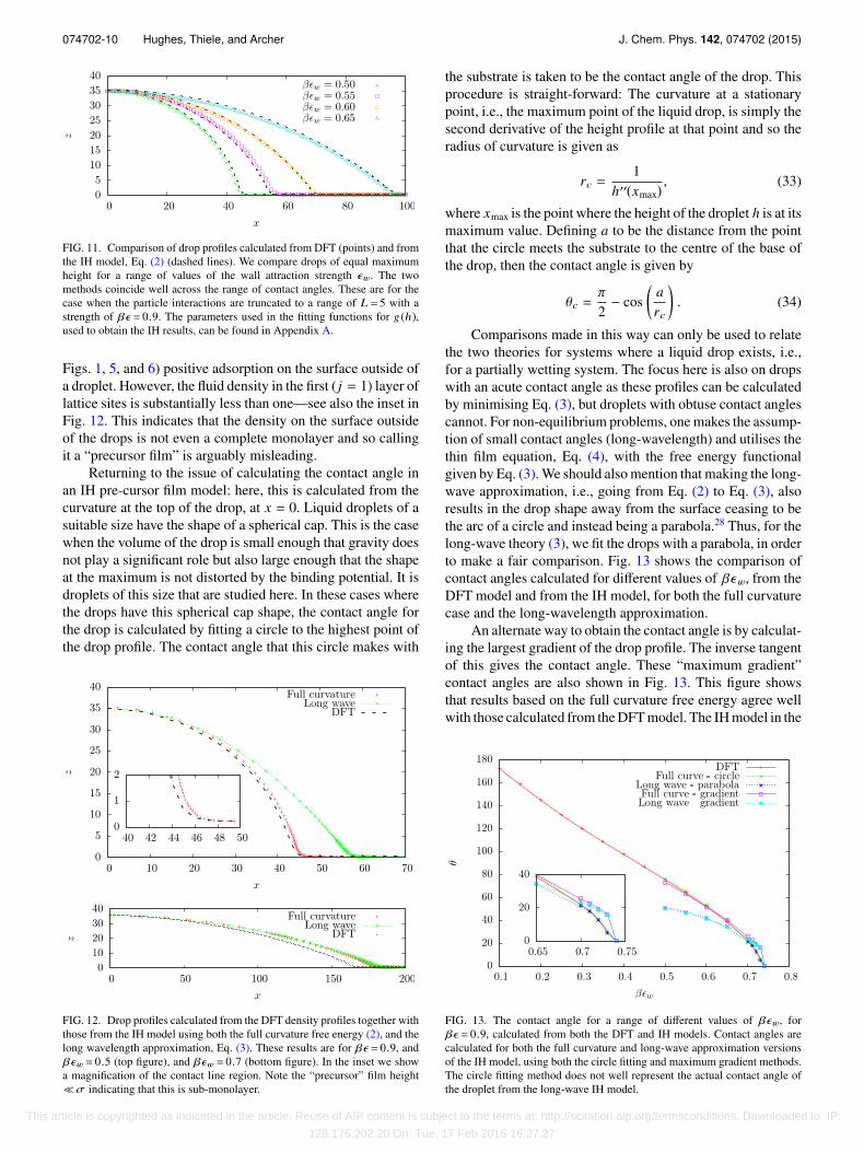
074702-10 Hughes, Thiele, and Archer J. Chem. Phys. 142, 074702 (2015)
FIG. 11. Comparison of drop profiles calculated from DFT (points) and fromthe IH model, Eq. (2) (dashed lines). We compare drops of equal maximumheight for a range of values of the wall attraction strength ϵw. The twomethods coincide well across the range of contact angles. These are for thecase when the particle interactions are truncated to a range of L = 5 with astrength of βϵ = 0.9. The parameters used in the fitting functions for g (h),used to obtain the IH results, can be found in Appendix A.
Figs. 1, 5, and 6) positive adsorption on the surface outside ofa droplet. However, the fluid density in the first ( j = 1) layer oflattice sites is substantially less than one—see also the inset inFig. 12. This indicates that the density on the surface outsideof the drops is not even a complete monolayer and so callingit a “precursor film” is arguably misleading.
Returning to the issue of calculating the contact angle inan IH pre-cursor film model: here, this is calculated from thecurvature at the top of the drop, at x = 0. Liquid droplets of asuitable size have the shape of a spherical cap. This is the casewhen the volume of the drop is small enough that gravity doesnot play a significant role but also large enough that the shapeat the maximum is not distorted by the binding potential. It isdroplets of this size that are studied here. In these cases wherethe drops have this spherical cap shape, the contact angle forthe drop is calculated by fitting a circle to the highest point ofthe drop profile. The contact angle that this circle makes with
FIG. 12. Drop profiles calculated from the DFT density profiles together withthose from the IH model using both the full curvature free energy (2), and thelong wavelength approximation, Eq. (3). These results are for βϵ = 0.9, andβϵw = 0.5 (top figure), and βϵw = 0.7 (bottom figure). In the inset we showa magnification of the contact line region. Note the “precursor” film height≪σ indicating that this is sub-monolayer.
the substrate is taken to be the contact angle of the drop. Thisprocedure is straight-forward: The curvature at a stationarypoint, i.e., the maximum point of the liquid drop, is simply thesecond derivative of the height profile at that point and so theradius of curvature is given as
rc =1
h′′(xmax) , (33)
where xmax is the point where the height of the droplet h is at itsmaximum value. Defining a to be the distance from the pointthat the circle meets the substrate to the centre of the base ofthe drop, then the contact angle is given by
θc =π
2− cos
(arc
). (34)
Comparisons made in this way can only be used to relatethe two theories for systems where a liquid drop exists, i.e.,for a partially wetting system. The focus here is also on dropswith an acute contact angle as these profiles can be calculatedby minimising Eq. (3), but droplets with obtuse contact anglescannot. For non-equilibrium problems, one makes the assump-tion of small contact angles (long-wavelength) and utilises thethin film equation, Eq. (4), with the free energy functionalgiven by Eq. (3). We should also mention that making the long-wave approximation, i.e., going from Eq. (2) to Eq. (3), alsoresults in the drop shape away from the surface ceasing to bethe arc of a circle and instead being a parabola.28 Thus, for thelong-wave theory (3), we fit the drops with a parabola, in orderto make a fair comparison. Fig. 13 shows the comparison ofcontact angles calculated for different values of βϵw, from theDFT model and from the IH model, for both the full curvaturecase and the long-wavelength approximation.
An alternate way to obtain the contact angle is by calculat-ing the largest gradient of the drop profile. The inverse tangentof this gives the contact angle. These “maximum gradient”contact angles are also shown in Fig. 13. This figure showsthat results based on the full curvature free energy agree wellwith those calculated from the DFT model. The IH model in the
FIG. 13. The contact angle for a range of different values of βϵw, forβϵ = 0.9, calculated from both the DFT and IH models. Contact angles arecalculated for both the full curvature and long-wave approximation versionsof the IH model, using both the circle fitting and maximum gradient methods.The circle fitting method does not well represent the actual contact angle ofthe droplet from the long-wave IH model.
This article is copyrighted as indicated in the article. Reuse of AIP content is subject to the terms at: http://scitation.aip.org/termsconditions. Downloaded to IP:
128.176.202.20 On: Tue, 17 Feb 2015 16:27:27

074702-11 Hughes, Thiele, and Archer J. Chem. Phys. 142, 074702 (2015)
long-wave approximation only agrees with the DFT results forvery small contact angles, as expected. For the full curvaturemodel, the contact angle found by fitting a circle to the profilematches the DFT results better than those from the maximumgradient method. The droplet shape calculated under the long-wavelength approximation is no longer that of a spherical cap,it is instead parabolic, and so a similar procedure to the circlefitting method is employed where a parabola is fitted to thedroplet profile. Results for the contact angle obtained via thesefits are shown in Fig. 13. Clearly, these results depend heavilyon the method used to find the contact angle of the droplets andalthough the circle/parabola fitting method gives better results,it is only applicable to specific drop shapes—see Ref. 22 for afurther discussion on extracting a contact angle from a dropprofile. Note also that the contact angles in Fig. 13 calculatedvia DFT are the only results to extend beyond 90; dropletprofiles cannot be found in this range using the IH model.
The calculated contact angles are weakly dependent onthe size of the drop. All contact angles extracted from the IHmodel are calculated from droplets that have a height of 35σ.Calculating contact angles from droplets of a specific height,rather than a specific volume, seems to give more consistentresults. The range at which particle interactions are truncateddoes not significantly affect how well the results from the twomodels (DFT an IH) agree with each other. Over the rangeof parameters studied, up to a truncation range of L = 40, thediscrepancy in the contact angle between the two models istypically a few percent.
VII. CONCLUSIONS
In this paper, we have developed a microscopic DFTbased method for calculating the binding potential g(Γ) atvarious different state points and interaction potentials ofvarious different strengths and ranges between the surfaceand the liquid. These were subsequently used as input to amesoscopic interface free energy model, which was then usedto calculate the height profile of liquid drops on surfaces. Theliquid height profiles are very similar in shape to the profilesobtained directly from the DFT, indicating that the coarse-graining procedure used to obtain g(Γ) is valid.
The binding potential is calculated as a function of theadsorption Γ, which can be related to the film height viaEq. (13). It is calculated using the method developed in Ref. 47for studying nucleation of the liquid from the gas phase. Thismethod constrains the fluid density profile to have a specifiedvalue of Γ, which is equivalent to imposing an additionalfictitious external potential that stabilises the adsorbed filmwith the given adsorption. Note that this fictitious potential isnot known a-priori and is calculated on-the-fly as part of theminimisation to obtain the fluid density profile.
The method presented for calculating the binding potentialis general and it should be possible to use if for any DFT. Here,it has been implemented using a simple DFT for a lattice-gas,that in Eq. (23). A better description of the free energy of alattice-gas is possible, we refer the interested reader to, e.g.,Ref. 57 for a more sophisticated and accurate approximationfor the lattice-gas free energy. The lattice-gas approximationwas used in order to more easily test the results for a range
of different drop sizes. Note that to calculate the 2D densityprofiles for drops of the size in Fig. 6 (or even larger) witha more sophisticated continuum DFT can be computationallytime consuming—e.g., using the commonly used approxima-tion F [ρ(r)] = FFMT[ρ(r)] + Fatt[ρ(r)], where FFMT[ρ(r)] isthe fundamental-measure theory approximation of the free en-ergy of a fluid of hard-spheres and Fatt[ρ(r)] is a simple mean-field approximation for the contribution to the free energy dueto the attractive interactions between the fluid particles.2,11–15
However, one of the draw-backs of the lattice-gas model is thatthe discretization onto a lattice leads to unrealistic small ampli-tude oscillations in g(Γ), particularly for larger values of βϵ(i.e., for lower temperatures)—see, e.g., Fig. 7. A more realisticcontinuum DFT model will not exhibit such oscillations thatdo not decay in amplitude with distance from the wall. Note,however, that oscillations may be present in the true bindingpotential. These, if present, stem from the packing of the parti-cles, rather than from the discretization onto a lattice and areto be expected whenever the fluid exhibits layering transitions.
Another drawback of the lattice-gas is that the mappingof the continuum fluid onto the lattice constitutes a signifi-cant approximation. This prevents a quantitative comparisonbetween our results with existing simulation results for con-tinuum models, such as those in Refs. 16–23. However, sincewe do find good qualitative agreement, we are currently apply-ing the method using continuum (FMT) DFT. Results fromthis follow-on study will be published elsewhere, includingcomparison with simulation results.
It should also be emphasised that it remains straight-forward to calculate droplet profiles using DFT rather thanusing the mesoscale model over the full range of contactangles, i.e., including when the contact angle >90. However,the IH model is particularly advantageous when consideringthe non-equilibrium situation, which can be described usingEq. (4), albeit this equation is derived under the assumption ofsmall contact angles and only accounts for convective transportwith no slip at the substrate. It is shown in Fig. 13 how theaccuracy rapidly breaks down for larger contact angles. Non-equilibrium phenomena can also be studied using dynamicalDFT, see, e.g., Refs. 58–61 for more on this approach.
One of the striking results of the present work is the obser-vation of the degree to which the binding potential changeswhen the range at which particle interactions are truncated ischanged—see in particular Figs. 8 and 9. Crucially, the valueof g(Γ) at the minimum that can be present at low values of theadsorption depends very sensitively on the truncation range.This minimum can change from being just a local minimum(a metastable equilibrium point) to become the global ener-getic minimum which represents a shift in the phase behaviourfrom wetting to non-wetting. In fact, for very short truncationranges, the minimum can be completely removed. The conclu-sion from this part of our study is that to determine accuratelythe location of a wetting transition in theory or simulations, onemust ensure that the truncation is not so severe as to induce sucherrors. The tails of the potentials matter!
This is important in the context of (coarse-grained) Molec-ular Dynamics simulations where dispersion forces are oftencut off at distances of a few particle diameters. Ref. 22, forinstance, employs a cut-off length for the Lenard Jones inter-
This article is copyrighted as indicated in the article. Reuse of AIP content is subject to the terms at: http://scitation.aip.org/termsconditions. Downloaded to IP:
128.176.202.20 On: Tue, 17 Feb 2015 16:27:27

074702-12 Hughes, Thiele, and Archer J. Chem. Phys. 142, 074702 (2015)
actions of two times the equilibrium bead distance and finds, inconsequence, that the extracted binding potential is well fittedby a sum of exponentials as in Eq. (17), similarly to our resultswhen only short-range interactions are considered.
Note also that for weakly attracting (solvophobic) walls,the minimum in g(Γ) is at very small, or potentially even nega-tive, values of Γ. In this regime, describing the sub-monolayeradsorption via a film-thickness h is a somewhat misleadingconcept. In this regime, the minimum in the binding potential isvery asymmetric, rising very sharply on the small Γ side of theminimum, but rising far less steeply as Γ is increased from thevalue at the minimum. To incorporate this behaviour in the fit-function for g(Γ), we had to use the exponential in the functionP(Γ) in Eq. (31). This also means that the minimum in g(Γ) isnot well-approximated by a quadratic function when the mini-mum is at a small value of Γ and so, of course, capillary-wavetheory also does not apply in this regime, since capillary-wavetheory assumes Gaussian fluctuations in a harmonic potential.Also, when the adsorption at the surface is sub-monolayer,then a non-equilibrium situation can no longer be describedby Eq. (4); it can instead be described via a gradient dynamicsmodel with a diffusive dynamics.
Finally, it should also be pointed out that although in thepresent work we have developed a method for calculating abetter approximation for the binding potential, our approach isstill a mean-field theory and therefore does not include all fluc-tuation effects, because our theory is based on Eq. (2). Some
effects of fluctuations at wetting transitions can be includedby replacing γlg in Eq. (2) with a function γ(h). However,as Parry and co-workers have showed, the effective interfaceHamiltonian is in fact non-local.62–64 Non-locality and fluc-tuation effects are particularly important at wetting transi-tions.
ACKNOWLEDGMENTS
A.P.H. acknowledges support through a LoughboroughUniversity Graduate School Studentship. All authors thank theCenter of Nonlinear Science (CeNoS) of the University ofMünster for recent support of the authors collaboration.
APPENDIX A: FIT FUNCTION PARAMETERS
Table I contains the parameters to the fitted binding poten-tials that have been used throughout this paper and also for aselection of other state points. For ease of reference, the fittingfunction is repeated here
g(Γ) = Aexp[−P(Γ)] − 1
Γ2 , (A1)
with
P(Γ) = a0Γ2e−a1Γ + a2Γ
2 + a3Γ3 + a4Γ
4 + a5Γ5 + a6Γ
6.
TABLE I. This table lists the parameters used in the fitting function to generate the results shown in the figures within the main text. The parameters areidentified by the figure in which the binding potential is used, the title of that curve in the figure, and some additional identification where applicable. Valuesare rounded to three decimal places and the value of a1 is enforced. For L = 5, the corresponding liquid gas surface tension values are βγlg = 0.111, 0.228 and0.351, for βϵ = 0.8, 0.9 and 1.0, respectively.
Figure βϵ βϵw L A a0 a1 a2 a3 a4 a5 a6
11 and 12 0.9 0.5 5 −0.073 1.142 8 −3.078 3.283 −1.272 0.173 0.00011 and 10 0.9 0.55 5 −0.081 1.080 8 −2.153 2.074 −0.705 0.084 0.00011 0.9 0.6 5 −0.088 0.964 8 −1.325 0.930 −0.036 −0.097 0.01911 0.9 0.65 5 −0.096 0.770 8 −0.534 −0.245 0.762 −0.358 0.05112 0.9 0.7 5 −0.103 0.609 8 0.138 −1.037 1.158 −0.451 0.060. . . 0.8 0.5 2 −0.062 0.431 8 0.431 −1.448 1.562 −0.649 0.097. . . 0.8 0.5 3 −0.062 0.562 8 −0.203 −0.900 1.175 −0.468 0.062. . . 0.8 0.5 4 −0.062 0.669 8 −0.473 −0.548 0.903 −0.363 0.047. . . 0.8 0.5 5 −0.062 0.776 8 −0.679 −0.222 0.634 −0.262 0.033. . . 0.8 0.5 10 −0.062 0.998 8 −1.035 0.415 0.107 −0.074 0.009. . . 0.8 0.5 20 −0.062 1.125 8 −1.194 0.752 −0.162 0.011 0.0001. . . 0.8 0.5 40 −0.062 1.104 8 −1.179 0.678 −0.100 −0.007 0.002. . . 0.9 0.6 2 −0.081 0.620 8 −0.108 −0.902 1.878 −1.093 0.228. . . 0.9 0.6 3 −0.088 0.786 8 −0.851 0.177 0.670 −0.405 0.068. . . 0.9 0.6 4 −0.096 0.824 8 −1.049 0.573 0.211 −0.182 0.030. . . 0.9 0.6 5 −0.102 0.823 8 −1.133 0.766 −0.019 −0.078 0.014. . . 0.9 0.6 10 −0.110 0.851 8 −1.273 1.023 −0.280 0.026 0.000. . . 0.9 0.6 20 −0.118 0.797 8 −1.234 0.965 −0.258 0.023 0.000. . . 0.9 0.6 40 −0.125 0.748 8 −1.170 0.898 −0.236 0.021 0.000. . . 1.0 0.65 2 −0.104 0.830 8 −1.186 1.224 0.172 −0.420 0.112. . . 1.0 0.65 3 −0.104 1.000 8 −1.961 2.217 −0.720 0.008 0.026. . . 1.0 0.65 4 −0.104 1.060 8 −2.232 2.584 −1.036 0.148 0.000. . . 1.0 0.65 5 −0.104 1.072 8 −2.385 2.718 −1.088 0.153 0.000. . . 1.0 0.65 10 −0.104 1.057 8 −2.594 2.863 −1.120 0.150 0.000. . . 1.0 0.65 20 −0.104 1.037 8 −2.646 2.882 −1.111 0.146 0.000. . . 1.0 0.65 40 −0.104 1.026 8 −2.658 2.880 −1.105 0.144 0.000
This article is copyrighted as indicated in the article. Reuse of AIP content is subject to the terms at: http://scitation.aip.org/termsconditions. Downloaded to IP:
128.176.202.20 On: Tue, 17 Feb 2015 16:27:27

074702-13 Hughes, Thiele, and Archer J. Chem. Phys. 142, 074702 (2015)
APPENDIX B: PARTICLE INTERACTION POTENTIALS
The net interaction potential between a fluid particle and aplanar wall made of particles interacting with the fluid particlevia a Lennard-Jones-like potential, with the same form as inEq. (21) is
Vi = ϵw f
0i′=−∞
∞j′=−∞
∞k′=−∞
((i − i′)2 + j ′2 + k ′2)−3, (B1)
where we assume the surface of the wall is located in theplane i = 0. The parameter ϵw f characterises the strength of theinteraction between a single wall particle and a fluid particle.The triple sum above spans all of the particles in the wall; i.e.,the wall is modelled as being discretised on a lattice just as thefluid is and that a wall particle is present on every lattice sitewhere i ≤ 0. The sums in Eq. (B1) can be simplified to obtain
Vi =
−ϵw/i3 for i ≥ 1∞ for i < 1
, (B2)
where the parameter ϵw determines the net strength of attrac-tion to the wall.
The (2D) effective fluid-fluid particle interactions are gov-erned in a similar manner by the potential
ϵ i,j = ϵ
(i′2 + j ′2)−3 + 2
∞k′=1
(i′2 + j ′2 + k ′2)−3. (B3)
The parameter ϵ is the strength of a single Lennard-Jones pairinteraction between two fluid particles and ϵ i,j is the weightedinteraction between two particles taking into account all of theinteractions in the invariant k dimension. In the right hand sideof Eq. (B3), i′, j ′, and k ′ are the distances between a pair oflattice sites in the i, j, and k directions, respectively.
Due to the fact that calculating long ranged particle inter-actions can be time consuming, making computer calculationsrather slow, it is often necessary to truncate the interactionsto some interaction range Lσ. When particle interactions aretruncated at a range of Lσ, the external potential Eq. (B1)becomes
Vi = ϵw f
0i′=−L
Lj′=−L
Lk′=−L
((i − i′)2 + j ′2 + k ′2)−3 for ((i − i′)2 + j ′2 + k ′2) ≤ L2
0 otherwise, (B4)
and the fluid-fluid particle interaction weights (B3) are then given as
ϵ i,j =
ϵ
(i′2 + j ′2)−3 + 2
k′≤√
L2−i′2− j′2k′=1
(i′2 + j ′2 + k ′2)−3
for |i − j| ≤ L
0 otherwise.
(B5)
1P. G. de Gennes, Rev. Mod. Phys 57, 827 (1985).2J.-P. Hansen and I. R. McDonald, Theory of Simple Liquids, 4th ed. (Elsevier,Warsaw, 2013).
3S. Dietrich, in Phase Transitions and Critical Phenemona, edited by C.Domb and J. Lebowitz (Academic Press, London, 1988), Vol. 12.
4M. Schick, Liquids at Interfaces, Proceedings of the Les Houches 1988Session XLVIII (Elsevier, 1988).
5L. MacDowell, J. Benet, and N. Katcho, Phys. Rev. Lett. 111, 047802 (2013).6L. MacDowell, J. Benet, N. Katcho, and J. Palanco, Adv. Colloid InterfaceSci. 206, 150 (2014).
7L. G. MacDowell, M. Müller, and K. Binder, Colloids Surf., A 206, 277(2002).
8J. R. Henderson, Phys. Rev. E 72, 051602 (2005).9M. Doi, Soft Matter Physics (Oxford University Press, 2013).
10R. Evans, Adv. Phys. 28, 143 (1979).11R. Evans, in Fundamentals of Inhomogeneous Fluids, edited by D.
Henderson (Taylor & Francis, 1992), Chap. 3, pp. 85–175.12J. Lutsko, in Adv. Chem. Phys., edited by S. Rice (John Wiley & Sons, Inc.,
Hoboken, NJ, USA, 2010).13P. Tarazona, J. Cuesta, and Y. Martínez-Ratón, in Lect. Notes Phys., edited
by A. Mulero (Springer, Berlin, Heidelberg, 2008), Vol. 753, Chap. 7,pp. 247–341.
14R. Evans, Lecture Notes, 3rd Warsaw School of Statistical Physics (WarsawUniversity Press, 2010).
15H. Löwen, Lecture Notes, 3rd Warsaw School of Statistical Physics (WarsawUniversity Press, 2010), pp. 87–121.
16L. G. MacDowell and M. Müller, J. Phys.: Condens. Matter 17, S3523(2005).
17L. G. MacDowell and M. Müller, J. Chem. Phys. 124, 084907 (2006).18A. Herring and J. Henderson, J. Chem. Phys. 132, 084702 (2010).19L. MacDowell, Eur. Phys. J.: Spec. Top. 197, 149 (2011).
20K. S. Rane, V. Kumar, and J. R. Errington, J. Chem. Phys. 135, 234102(2011).
21R. de Gregorio, J. Benet, N. A. Katcho, F. J. Blas, and L. G. MacDowell, J.Chem. Phys. 136, 104703 (2012).
22N. Tretyakov, M. Müller, D. Todorova, and U. Thiele, J. Chem. Phys. 138,064905 (2013).
23J. Benet, J. G. Palanco, E. Sanz, and L. G. MacDowell, J. Phys. Chem. C118, 22079 (2014).
24A. Oron, S. H. Davis, and S. G. Bankoff, Rev. Mod. Phys 69, 931 (1997).25U. Thiele, in Thin films of soft matter, edited by S. Kalliadasis and U.
Thiele (Springer, Wien, New York, 2007), pp. 25–94.26V. S. Mitlin, J. Colloid Interface Sci. 156, 491 (1993).27U. Thiele, J. Phys.: Condens. Matter 22, 084019 (2010).28S. A. Safran, Statistical Thermodynamics of Surfaces, Interfaces and Maem-
branes (Addison-Wesley, Reading, MA, 1994).29G. Berim and E. Ruckenstein, J. Chem. Phys. 129, 014708 (2008).30E. Ruckenstein and G. Berim, Adv. Colloid Interface Sci. 157, 1 (2010).31A. Pereira and S. Kalliadasis, J. Fluid Mech. 692, 53 (2011).32A. Nold, A. Malijevský, and S. Kalliadasis, Eur. Phys. J.: Spec. Top. 197,
185 (2011).33A. Nold, D. Sibley, B. Goddard, and S. Kalliadasis, Phys. Fluids 26, 072001
(2014).34A. Marchand, J. H. Weijs, J. H. Snoeijer, and B. Andreotti, Am. J. Phys. 79,
999 (2011).35N. Churaev, Adv. Colloid Interface Sci. 58, 87 (1995).36M. Rauscher and S. Dietrich, Annu. Rev. Mater. Res. 38, 143 (2008).37R. Evans, Proceedings of the Les Houches 1988 Session XLVIII (Elsevier,
1989).38I. Ibagon, M. Bier, and S. Dietrich, J. Chem. Phys. 138, 214703 (2013).39I. Ibagon, M. Bier, and S. Dietrich, J. Chem. Phys. 140, 174713 (2014).40M. C. Stewart and R. Evans, J. Phys.: Condens. Matter 17, S3499 (2005).
This article is copyrighted as indicated in the article. Reuse of AIP content is subject to the terms at: http://scitation.aip.org/termsconditions. Downloaded to IP:
128.176.202.20 On: Tue, 17 Feb 2015 16:27:27

074702-14 Hughes, Thiele, and Archer J. Chem. Phys. 142, 074702 (2015)
41E. M. Fernández, E. Chacón, and P. Tarazona, Phys. Rev. B 85, 205435(2011).
42E. Brézin, B. I. Halperin, and S. Leibler, J. Physique 44, 775 (1983).43R. Evans and J. Henderson, J. Phys.: Condens. Matter 21, 474220
(2009).44L. Frastia, A. J. Archer, and U. Thiele, Soft Matter 8, 11363 (2012).45A. P. Hughes, U. Thiele, and A. J. Archer, Am. J. Phys. 82, 1119 (2014).46R. Roth, J. Phys.: Condens. Matter 22, 063102 (2010).47A. Archer and R. Evans, Mol. Phys. 109, 2711 (2011).48A. J. Archer and R. Evans, J. Chem. Phys. 138, 014502 (2013).49M. J. Robbins, A. J. Archer, and U. Thiele, J. Phys.: Condens. Matter 23,
415102 (2011).50A. Malijevský and A. Archer, J. Chem. Phys. 139, 144901 (2013).51F. Detcheverry, E. Kierlik, M. L. Rosinberg, and G. Tarjus, Phys. Rev. E 68,
061504 (2003).52F. Porcheron and P. A. Monson, Langmuir 22, 1595 (2006).53P. A. Monson, J. Chem. Phys. 128, 084701 (2008).54S. Dietrich and M. Napiórkowski, Phys. Rev. A 43, 1861 (1991).55A. J. Archer, J. Phys.: Condens. Matter 18, 5617 (2006).56A. J. Archer, J. Chem. Phys. 130, 014509 (2009).57J. R. Edison and P. A. Monson, J. Chem. Phys. 141, 024706 (2014).58U. M. B. Marconi and P. Tarazona, J. Chem. Phys. 110, 8032 (1999).59U. M. B. Marconi and P. Tarazona, J. Phys.: Condens. Matter 12, A413
(2000).60A. Archer and R. Evans, J. Chem. Phys 121, 4246 (2004).
61A. Archer and M. Rauscher, J. Phys. A: Math. Gen. 37, 9325 (2004).62A. O. Parry, C. Rascón, N. R. Bernardino, and J. M. Romero-Enrique, J.
Phys.: Condens. Matter 18, 6433 (2006).63A. O. Parry, C. Rascón, N. R. Bernardino, and J. M. Romero-Enrique, J.
Phys.: Condens. Matter 19, 416105 (2007).64N. R. Bernardino, A. O. Parry, C. Rascón, and J. M. Romero-Enrique, J.
Phys.: Condens. Matter 21, 465105 (2009).65Note that the contribution to the lattice gas free energy densityβ f = ρ ln ρ − (1 − ρ) ln(1 − ρ) in Eq. (23) contains both the ideal gasβ fid = ρ ln ρ − ρ and an excess contribution β fex = ρ + (1 − ρ) ln(1− ρ); i.e., f = fid + fex. The origin of this form arises from the hole-particle ni↔ 1 − ni symmetry in the lattice model (see, e.g., Ref. 45). Thesecond term, fex, stems from the particles having a hard-core interaction,preventing multiple occupancy of a cell. It is instructive to compare thiswith the free energy of a binary mixture. The ideal-gas contribution tothe free energy of a mixture is β f = ρ1 ln ρ1 − ρ1 + ρ2 ln ρ2 − ρ2, whereρ1 is the density of species 1 and ρ2 the density of species 2. Re-writing this in terms of the total density ρ = ρ1 + ρ2 and concentrationx = ρ1/ρ, we obtain β f = ρ ln ρ − ρ + ρ[x ln x + (1 − x) ln(1 − x)]. Thefinal term is the ideal-gas contribution to the entropy of mixing and it isinteresting to note the similarity in form to the lattice-gas free energy. Foran incompressible binary mixture, ρ is a constant and so the first twoterms are often neglected. As a consequence of this, the free energy of anincompressible binary fluid can have a very similar mathematical form tothe lattice-gas free energy considered here.
This article is copyrighted as indicated in the article. Reuse of AIP content is subject to the terms at: http://scitation.aip.org/termsconditions. Downloaded to IP:
128.176.202.20 On: Tue, 17 Feb 2015 16:27:27


