“Liquidation” Cycles and the Great Depression * J. Bradford De Long Harvard University and NBER first draft March 1989; this draft June 1991 The Federal Reserve took almost no steps to halt the slide into the Great Depression over 1929–33. Instead, the Federal Reserve acted as if appropriate policy was not to try to avoid the oncoming Great Depression, but to allow it to run its course and “liquidate” the unprofitable portions of the private economy. In adopting such “liquidationist” policies, the Federal Reserve was merely following the recommendations provided by an economic theory of depressions that was in fact common before the Keynesian Revolution and was held by economists like Friedrich Hayek, Lionel Robbins, and Joseph Schumpeter. This paper reconstructs the logic of this “liquidationist” view, and argues that the perspective was carefully thought out (although not adequate to the Depression) and may have held some truth as applied to business cycles that came before the Great Depression. The inaction of the United States government during the 1929–33 slide into the Great Depression is both astonishing and puzzling when viewed from any of the perpectives held today. All points of view today hold that governments should strive to provide a stable environment in which the private economy can operate, and should do this by keeping some broad nominal aggregate measure of spending or liquidity on a stable growth path. For monetarist economists, the measure to be stabilized is some definition of the nominal money supply. 1 For Keynesians, the appropriate aggregate is total nominal demand itself. 2 As the conduct of economic policy while a depression is pending is concerned, these differences of opinion are relatively minor, for they all teach one central lesson: the central bank should pour reserves and liquidity into the banking system as fast as * I wish to thank John Leahy, Murray Milgate, Robert Waldmann, and especially Barry Eichengreen and Randy Kroszner for helpful discussions, and Hoang Quan Vu for enthusiastic research assistance. 1 See Milton Friedman (1984). 2 See Robert Hall and John Taylor, Macroeconomics
Transcript
“Liquidation” Cycles and the Great Depression*
J. Bradford De LongHarvard University and NBER
first draft March 1989;this draft June 1991
The Federal Reserve took almost no steps to halt the slide into the GreatDepression over 1929–33. Instead, the Federal Reserve acted as if appropriatepolicy was not to try to avoid the oncoming Great Depression, but to allow it torun its course and “liquidate” the unprofitable portions of the private economy.In adopting such “liquidationist” policies, the Federal Reserve was merelyfollowing the recommendations provided by an economic theory of depressionsthat was in fact common before the Keynesian Revolution and was held byeconomists like Friedrich Hayek, Lionel Robbins, and Joseph Schumpeter. Thispaper reconstructs the logic of this “liquidationist” view, and argues that theperspective was carefully thought out (although not adequate to the Depression)and may have held some truth as applied to business cycles that came before theGreat Depression.
The inaction of the United States government during the 1929–33 slide into the
Great Depression is both astonishing and puzzling when viewed from any of the
perpectives held today. All points of view today hold that governments should strive to
provide a stable environment in which the private economy can operate, and should do
this by keeping some broad nominal aggregate measure of spending or liquidity on a
stable growth path. For monetarist economists, the measure to be stabilized is some
definition of the nominal money supply.1 For Keynesians, the appropriate aggregate is
total nominal demand itself.2
As the conduct of economic policy while a depression is pending is concerned,
these differences of opinion are relatively minor, for they all teach one central lesson:
the central bank should pour reserves and liquidity into the banking system as fast as
*I wish to thank John Leahy, Murray Milgate, Robert Waldmann, and especially Barry Eichengreen andRandy Kroszner for helpful discussions, and Hoang Quan Vu for enthusiastic research assistance.1See Milton Friedman (1984).2See Robert Hall and John Taylor, Macroeconomics
Wednesday, August 5, 1998 2 “Liquidation” Cycles and the Great Depression
possible3 in order to keep the money stock and demand from collapsing during
depressions. Above all, the central bank should not aggravate depressions by
unexpectedly imposing contractionary policy on an already weakening economy.
This, however, was not the policy followed during the Great Depression.4 The
Federal Reserve did not push reserves into the banking system during the 1929–33
decline. It passively stood by while the nominal money stock fell by a third. The federal
govenment did not increase its spending while allowing its tax revenues to fall. Instead,
strenuous efforts were made to balance the budget and keep it balanced.
These policies were disastrous. They certainly did not stop the contraction in
economic activity. They may well have severely aggravated it, and presumably played
an important role in making the 1929–41 depression into the Great Depression.
Alternatives were considered. Factions within the Federal Reserve system did argue for
expanding liquidity during the downslide.5 They were overruled by those who thought
that the economy needed to go through a period of “liquidation” in order to lay the
groundwork for renewed expansion. “Liquidationists” pointed to the short (but sharp)
1921 recession, argued that it had laid the groundwork for prosperity in the 1920’s, and
pushed for similar deflationary policies—which they mistakenly hoped would assist the
release of capital and labor from unproductive activities, and lay the groundwork for a
similar boom in the 1930’s.6
The current of mind that underlay “liquidationism” was not a freak belief held
by central bankers and makers of policy alone. Such a “liquidationist” theory of the
function of depressions was in fact a common position for economists to take before the
Keynesian Revolution, and was held and advanced by economists as eminent as Hayek,
3And the fiscal authorities should cut taxes and accelerate spending as much as necessary.4See among others Milton Friedman and Anna Schwartz, A Monetary History of the United States, LesterChandler, America’s Greatest Depression, Peter Temin, Did Monetary Forces Cause the Great Depression? andLessons from the Great Depression, Barry Eichengreen, Golden Fetters: The Gold Standard and the GreatDepression, and Charles Kindleberger, The World in Depression 1929–1939.5Friedman and Schwartz, Monetary History, Epstein and Ferguson, “Loan Liquidation…“ Temin, Lessonsfrom the Great Depression.6Barry Eichengreen, Golden Fetters: The Gold Standard and the Great Depression.
Wednesday, August 5, 1998 3 “Liquidation” Cycles and the Great Depression
Robbins, and Schumpeter. In squeezing an already-weak economy, the makers of
American economic policy were to some degree acting as John Maynard Keynes
believed that policy makers always act: they were “madmen in authority” obeying
voices in the air which were to some degree echoes of academic debates.7 Academic
economics gave central bankers a warrant for their contractionary depression-era
policies.
In the aftermath of the Great Depression, the intellectual rout of the
liquidationists and the victory of the Keynesians was complete. Pre-Keynesian business
cycle theory receives less than a footnote in post-World War II macroeconomic texts.8
This paper reconstructs the logic of the “liquidationist” view. Its first substantive
section sets out their main articles of belief. Its second section presents a simple model
in the tradition of their vision—in which depressions are unpleasant but unavoidable
episodes in the growth of a dynamic economy facing an uncertain future, in which
attempts to use expansionary policies to keep investment high in a depression are
positively destructive and inimical to the general welfare, and in which high
unemployment in a depression is really a sign that the market economy is doing its job
and is the best conceivable social mechanism for controlling production and
distribution. And a third section speculates on the origins of “liquidationism.”
These tasks are worth carrying out for at least reasons. First, it is worthwhile to
do the history of economic thought right. Previous generations of economists were as
smart and keen sighted as the present generation. To understand what they believed,
and why they believed it, sheds light on the actual workings of economies and on
economists’ present beliefs.
Second, the existence of “liquidationism” played a key part in motivating public
policy decisions not to fight the gathering Great Depression. The history of economic
policy and economic activity in the Great Depression cannot be done right unless done
7John Maynard Keynes, The General Theory of Employment, Interest and Money (London: Macmillan, 1936).8One of the few exceptions is Salant (1989).
Wednesday, August 5, 1998 4 “Liquidation” Cycles and the Great Depression
against the background of the “liquidationist” perspective that so many influential
people—cabinet officers, central bankers, academics, and so on—held.
I. The Great Depression and the “Liquidationist” Perspective
From late summer 1929 up to the inauguration of Roosevelt, all macroeconomic
indicators in the United States signalled what modern economists would see as a grave
and immediate need for expansion. The stock market declined in nominal terms at 35
percent, and in real terms at 25 percent per year. The price level and the nominal money
stock both fell at about 8 percent per year. A flight to quality pushed interest rates on
government securities and on short-run paper issued by the most credit-worthy firms
down, while the nominal interest rates at which corporations could borrow for the long
term rose.9
Economic Policy Under Hoover
Throughout this decline—which carried real GNP per worker down to a level 40
percent below that which it had attained in 1929, and which saw the unemployment rise
to take in more than a quarter of the labor force—the government did not try to prop up
aggregate demand. The only expansionary fiscal policy action undertaken was the
Veterans’ Bonus, passed over President Hoover’s veto.10 That aside, the full-
employment budget surplus did not fall over 1929–33.11
9Peter Temin, Did Monetary Forces Cause the Great Depression?10Chandler, America’s Greatest Depression.11E. Cary Brown, “Fiscal Policy in the Thirties: A Reappraisal,” American Economic Review 46 (December1956), pp. 857–79.
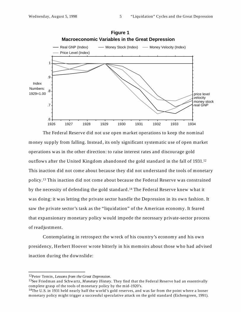
Wednesday, August 5, 1998 5 “Liquidation” Cycles and the Great Depression
.6
.7
.8
.9
1
1926 1927 1928 1929 1930 1931 1932 1933 1934
Real GNP (Index)
Price Level (Index)
Money Stock (Index) Money Velocity (Index)
IndexNumbers:1929=1.00
Figure 1Macroeconomic Variables in the Great Depression
price levelvelocitymoney stockreal GNP
The Federal Reserve did not use open market operations to keep the nominal
money supply from falling. Instead, its only significant systematic use of open market
operations was in the other direction: to raise interest rates and discourage gold
outflows after the United Kingdom abandoned the gold standard in the fall of 1931.12
This inaction did not come about because they did not understand the tools of monetary
policy.13 This inaction did not come about because the Federal Reserve was constrained
by the necessity of defending the gold standard.14 The Federal Reserve knew what it
was doing: it was letting the private sector handle the Depression in its own fashion. It
saw the private sector’s task as the “liquidation” of the American economy. It feared
that expansionary monetary policy would impede the necessary private-sector process
of readjustment.
Contemplating in retrospect the wreck of his country’s economy and his own
presidency, Herbert Hoover wrote bitterly in his memoirs about those who had advised
inaction during the downslide:
12Peter Temin, Lessons from the Great Depression.13See Friedman and Schwartz, Monetary History. They find that the Federal Reserve had an essentivallycomplete grasp of the tools of monetary policy by the mid-1920’s.14The U.S. in 1931 held nearly half the world’s gold reserves, and was far from the point where a loosermonetary policy might trigger a successful speculative attack on the gold standard (Eichengreen, 1991).
Wednesday, August 5, 1998 6 “Liquidation” Cycles and the Great Depression
The ‘leave-it-alone liquidationists’ headed by Secretary of theTreasury Mellon…felt that government must keep its hands off andlet the slump liquidate itself. Mr. Mellon had only one formula:‘Liquidate labor, liquidate stocks, liquidate the farmers, liquidatereal estate’.…He held that even panic was not altogether a badthing. He said: ‘It will purge the rottenness out of the system. Highcosts of living and high living will come down. People will workharder, live a more moral life. Values will be adjusted, andenterprising people will pick up the wrecks from less competentpeople’.15
But “liquidationism” was not the creation and responsibility of a cabal of cabinet
members headed by Andrew Mellon. The Hoover administration’s and the Federal
Reserve’s unwillingness to use policy to prop up aggregate demand during the slide
into the Depression was approved by eminent economists of the day. From Harvard,
Seymour Harris argued that just because the banking system was near collapse was no
reason for the Federal Reserve to buy bonds for cash: “Open market operations are not
the most effective method of dealing with… bank failures, any more than the proper
way of filling numerous small holes on the surface of the earth is to flood the earth with
water.”16 Also from Harvard, Joseph Schumpeter argued that there was a “presumption
against remedial measures which work through money and credit.… policies of this
class are particularly apt to…produce additional trouble for the future.”17 Similar calls
to avoid attempts to use economic policy to ameliorate the depression came from many
other eminent economists: Robertson, Hayek, Robbins, and others. “Liquidationism”
saw itself, in Robbins’ words, as “a point of view…[that was] the heritage of generations
of subtle and disinterested thought” and that saw much further to the core of what was
going on in the economy than other perspectives.18
Where to look to find the economists’ argument? It is an old principle that to
15Hoover, 1952, vol. 3, p. 30. Quoted in Wiseley (1977), p. 118, and then requoted in Kindleberger (1978),pp. 139–40.16Seymour Harris, 1934, p. 104.17Schumpeter, 1934; p. 20.18Lionel Robbins, The Great Depression (London: Macmillan, 1935), p. vii.
Wednesday, August 5, 1998 7 “Liquidation” Cycles and the Great Depression
ascertain the underlying theoretical vision it is best to avoid writings on theory and to
instead examine writings on policy. Writings on theory are discursive. They are hedged
with qualifications, exemptions, and elaborations. Writings on policy are compact. The
intended audience is made up not of academics with time to think and read but of busy
men of affairs. Such writings are much more disciplined. The author fears that those
reading his message may soon flip the page, and so he strains every nerve to make sure
that the points that are made are the central and important points and that they are
made clearly and convincingly.19
In 1934 a group of the Harvard Economics faculty wrote and published a short
book, edited by Douglass Brown, entitled The Economics of the Recovery Program.20 These
academic economists saw their book as an attempt to intervene in politics. They, who
had long studied the economy, would try to convey in a brief space what had gone
wrong to land the economy in its Great Depression, and how the recovery should be
managed.
Joseph Schumpeter took on the task of writing the chapter on what business
cycles and depressions really were. Thus he wrote Schumpeter (1934), which gives the
clearest exposition of the “liquidationist” line of argument that was believed by Mellon,
other makers of policy, and other economists like Hayek (1931, 1935),21 Harris (1934),
and Robbins (1935).
19For example, Friedrich Hayek’s business cycle theory is almost impossible to grasp from his theoreticalworks, like Prices and Production. Hayek uses an “Austrian” analytical apparatus that was built as a toolfor anti-Marxist capital theory. But when he is trying to reach a larger audience, and to compress hismessage into a small space, it comes through clearly. Consider the passage from The Road to Serfdom(Chicago: University of Chicago Press, 1947) infra.20I owe my knowledge of this source to Charles Kindleberger.21“Austrian” economists were not the only source, even though they were one source, of liquidationistdoctrines. “Austrian” attempts to develop formal business cycle theories, however, did not mesh wellwith their approach to capital theory and the determination of the rate of interest. The businessmen’spoint of view as laid out by Mellon, and the frameworks sketched out by Robbins and Schumpeter areflawlessly transparent compared to the opaque theoretical writings of Hayek. The same holds true, to alesser degree, for Schumpeter: it is more difficult to determine why Schumpeter believes the GreatDepression happened by reading his two-volume, seven-hundred page 1939 Business Cycles than byreading his thirty page 1934 “Depressions.”
Wednesday, August 5, 1998 8 “Liquidation” Cycles and the Great Depression
The Liquidationist Argument
Schumpeter begins from the observation that the course of economic
development is never smooth. Investments and enterprises are gambles on the future,
made by innovative entrepreneurs who see new things to be done or new ways to
produce old commodities. Sometimes these gambles will fail. The actual future that
comes to pass is one in which ex post certain investments should not have been made, or
in which ex post certain enterprises should not have been undertaken because they are
not producing the requisite profits. The economy is left with “too much” capital given
what the state of technology factor supplies, and demand turned out to be, or is perhaps
left with the “wrong kinds” of capital.
The best that can be done in such a situation is to shut down those production
processes and enterprises that were based on guesses about the way the future would
look that did not come to pass. The liquidation of investments and businesses releases
factors from unprofitable uses; they can then be redeployed to other sectors, used to
produce socially useful current services (in the “too much” capital case) or alternative
investment goods (in the “wrong kinds” case), and used by further waves of
entrepreneurs in new gambles on a still-uncertain future. But without the initial
liquidation, the redeployment and the subsequent wave of innovation and
entrepreneuship cannot take place.
It follows, says Schumpeter, that depressions are this process of liquidation and
preparation for the redeployment of resources. From Schumpeter’s perspective,
“depressions are not simply evils, which we might attempt to suppress, but…forms of
something which has to be done, namely, adjustment to…change.” This socially
productive function of depressions creates “the chief difficulty” faced by economic
policy makers. For “most of what would be effective in remedying a depression would
be equally effective in preventing this adjustment” (Schumpeter, 1934; p. 16). The
process of dynamic economic growth requires that underutilized factors register their
availability on markets. Policies that stimulate demand in recessions keep factors
Wednesday, August 5, 1998 9 “Liquidation” Cycles and the Great Depression
engaged in activities that do not produce value in excess of social cost. Such policies
keep factor markets from registering the potential availability of productive resources
for redeployment.
Is it possible to iron out the cycles, leaving an economy growing steadily on some
equilibrium path rather than irregularly with rapid booms and slumps? Schumpeter
thinks not. The preface to his Business Cycles(New York: McGraw-Hill, 1939) stresses
that business cycles are not “…like tonsils, separable things that might be treated by
themselves.” It asserts that business cycles are “…like the beat of the heart, of the
essence of the organism that displays them” (p. v). In order for one wave of
entrepreneurship to be followed by another, prospective entrepreneurs must know
where and in what quantities resources available for recombination and redeployment
are available. Until they can learn this, they face “the imposibility of calculating costs
and receipts in a satisfactory way…[T]he diffculty of planning new things and the risk
of failure are greatly increased.…[I]t is necessary to wait until things settle
down…before embarking on [new] innovation” (pp. 135–6).
Schumpeter argues that monetary policy does not allow policy makers to choose
between depression and no depression, but between depression now and a worse
depression later. “Inflation…pushed far enough [would] undoubtedly turn depression
into the sham prosperity so familiar from European postwar experience,” claims
Schumpeter. But, he goes on to say, it “would, in the end, lead to a collapse worse than
the one it was called in to remedy” (Schumpeter, 1934; p. 16).
Hence his “…analysis leads us to believe that recovery is sound only if it does
come of itself. For any revival which is merely due to artificial stimulus leaves part of
the work of depressions undone and adds, to an undigested remnant of maladjustment,
new maladjustment of its own which has to be liquidated in turn, thus threatening
business with another [worse] crisis ahead” (Schumpeter, 1934; p. 20).
Since the basic maladjustment is past investments and lines of business that have
turned out to be socially unproductive and in need of liquidation, the “trouble is
Wednesday, August 5, 1998 10 “Liquidation” Cycles and the Great Depression
fundamentally not with money and credit,” but with past overinvestment. Stimulative
monetary policies, therefore, “are particulary apt to keep up, and add to,
maladjustment, and to produce additional trouble for the future” (Schumpeter, 1934; p.
20). Moreover, words like “stimulative” carry a special meaning in this context: if
private sector actions would lead to a fall in, say, the nominal money stock, then a
public sector attempt to counteract the consequences of such private-sector actions by
injecting sufficient reserves to hold the nominal money stock constant would be
“stimulative.”
Hayek’s (1931) rejection of expansionary policies is the same argument: the belief
“that a general crisis can be averted by extension of credit” is a “popular fallacy.”
Moreover, “the great expectations attached to…public works in times of depression
[are]…fallacious,” for public works also “bring about all those evil effects which…arise
when [the] money [supply] is increased.” His conclusion, expressed most clearly in his
1944 Road to Serfdom, is that even if the economy could be stabilized at full employment
this would not be good policy:
This problem [of unemployment]…is one which will always bewith us so long as the economic system has to adopt itself tocontinuous changes. There will always be a possible maximum ofemployment in the short run which can be achieved by giving allpeople employment where they happen to be and which can beachieved by monetary expansion…but…with the effect of holdingup those redistributions of labor between industries madenecessary by…changed cicumstances.…[T]o aim always at themaximum of employment achievable by monetary means is apolicy which is certain in the end to defeat its own purposes… andlower productivity (p. 208).
In some ways, Hayek was a moderate. Lionel Robbins (1934) went so far as to
attribute the extraordinary depth and length of the Great Depression to excessive
expansionary monetary policy. He wrote that: “The moment the boom broke…Central
Banks of the world… set to work to create a condition of easy money.…The process of
liquidation was arrested.” This was a mistake. For:
Wednesday, August 5, 1998 11 “Liquidation” Cycles and the Great Depression
[i]n…a boom many bad business commitments are undertaken.…[Goods] are produced…which it is impossible to sell at a profit.Loans are made which it is impossible to recover.…[W]hen theboom breaks, these …commitments are revealed.…Nobodywishes… bankruptcies. Nobody likes liquidation as such.… [But]when the extent of mal-investment and over-indebtedness haspassed a certain limit, measures which postpone liquidation onlymake matters worse (Robbins, 1935, pp. 72–5).
Robbins’ diagnosis was that the world economy in the 1930’s needed more, not less
deflation: “In the present depression we eschew the sharp purge. We prefer the
lingering disease.” He thought that a significant opportunity had been lost because of
governmental unwillingness to impose a real deflation in 1930. He thought it a pity that
“a more astringent policy in 1930” had not been followed. For he thought it would have
quickly liquidated the backlog of excess investment and unsound enterprise, and would
have been unlikely “to cause more disturbance and dislocation than…have actually
been caused by [liquidation’s] postponement.”
In abstract theory there is no a priori reason for the redistributions of labor and
machines from socially unproductive to socially productive lines of enterprise to
require prolonged unemployment and idle capacity. Frictions in markets—labor unions,
relocation costs, imperfect information, and so forth—mean that this process of
reallocation entails unemployment, slack capacity, and temporarily reduced
production. Before entrepreneurs in lines of business that should expand become aware
of the availability of additional factors, such factors must be released from their past
uses. They spend time in “inventory” while their availability for redeployment registers
on the supply side of the marketplace. Thus Robbins and Schumpeter argued that
appropriate policy was not to try to pump up aggregate demand and so stop the
process of liquidation and reallocation: that process would have to be carried through
eventually; postponing it simply magnified the social costs.22
22Note that the Schumpeterian argument can look with favor on welfare state policies likeunemployment insurance. Since all benefit from the redeployments that take place as a result ofunemployment, it is inefficient for workers rendered unemployed to bear the entire cost of lost incomesince they do not reap the subsequent benefits.
Wednesday, August 5, 1998 12 “Liquidation” Cycles and the Great Depression
Dissent from Liquidationism
This doctrine—that in the long run the Great Depression would turn out to have
been “good medicine” for the economy, and that proponents of stimulative policies
were shortsighted enemies of the public welfare—drew anguished cries of dissent from
others. The British economist Ralph Hawtrey scorned those who, like Robbins, wrote at
the nadir of the Great Depression that the greatest danger the economy faced was
inflation. To call for more liquidation and deflation was, Hawtrey said, “to cry, ‘Fire!
Fire!’ in Noah’s flood.”23 Milton Friedman (1974) recalled that at Knight, Simons, and
Viner’s Chicago such dangerous nonsense was not taught, but he understood why at
Harvard—where such nonsense was taught—bright young graduate student
economists might rebel, reject their teachers’ macroeconomics, and become
Keynesians.24 Keynesianism might be false but it was not insane, and it was not as false
as what graduate students were being taught by Schumpeter.
John Maynard Keynes himself (1931) tried to discredit the “liquidationist view”
with the rhetoric of ridicule. He called it an “imbecility” to argue that the “wonderful
outburst of productive energy” during the boom of 1924–29 had made the Great
Depression inevitable. He spoke of Hayek, Robbins, Schumpeter, and their fellow
travelers as:
…austere and puritanical souls [who] regard [the GreatDepression] …as an inevitable and a desirable nemesis on…“overexpansion” as they call it.…It would, they feel, be a victoryfor the mammon of unrighteousness if so much prosperity was notsubsequently balanced by universal bankruptcy. We need, they say,what they politely call a ‘prolonged liquidation’ to put us right. Theliquidation, they tell us, is not yet complete. But in time it will be.And when sufficient time has elapsed for the completion of theliquidation, all will be well with us again… (Keynes, 1972; vol. XIII,pt. 1, p. 349)
23I owe this quotation to Peter Temin.24Friedman’s report on the state of Chicago thought during the early stages of the Depression issupported by Davis (1971); it is challenged by Patinkin (1978) and by Johnson (1969).
Wednesday, August 5, 1998 13 “Liquidation” Cycles and the Great Depression
In spite of some opposition, the “liquidationist” view carried the day over
virtually the entire world during 1929–33, and over much of the world during 1933–39.
Even governments that had unrestricted international freedom of action—like France
and the United States with their massive gold reserves, and like Britain after its
departure from the gold standard—tended not to pursue expansionary monetary and
fiscal policies on the grounds that such would reduce investor “confidence” and hinder
the process of liquidation, reallocation, and the resumption of private investment (see
Temin, 1989; Eichengreen, 1991; Hall, ed., 1989).
The Eclipse of the “Liquidationist” View
After the Great Depression and World War II the victory of the Keynesians was
complete. Nothing was left of the doctrines of “liquidationists”—it was not easy to learn
what the doctrines had been.25 Post-World War II courses in macroeconomics did not
teach how modern theories were better than, or even what the theories of their
predecessors had been.26 They proceeded in logical sequence, not in historical sequence,
from a model of full-employment Walrasian equilibrium to one with Keynesian (or
monetarist) cycles (Patinkin, 1982).
The business cycle theories that had held sway before the Keynesian revolution
were dealt with only in asides. Miton Friedman (1974) speaks of how outside of
Chicago interwar macroeconomics was dominated an “atrophied and rigid caricature of
the quantity theory” that could not guide economic policy. Keynesians like Galbraith
25Salant (1989) is one of the few chroniclers of the Keynesian revolution who refers to “liquidationism,”calling it the “‘crime and punishment’ theory of business cycles.26Dim echos of some “liquidationist” concerns can be heard in some of the internal debate withinmonetarism over which monetary aggregate to stabilize. For the early Friedman (1974), this was anempirical question: which monetary aggregate is the best leading indicator of total nominal demand? Forothers like Brunner and Meltzer (1974), or like the later Friedman (1984), this was a theoretical question:stabilizing which monetary aggregate corresponds to the government’s not distorting private-sectorincentives?
Pre-Keynesian debates over just what a “neutral” monetary policy was could become highlyscholastic. Hayek (1931), for example, sees a world of difference between a policy that stabilizes thenominal stock of outside money and one that maintains a stable price level. The second, he believes,distorts private-sector incentives and inevitably paves the way for crises and depressions—he saw one ofhis major intellectual tasks as the overthrow of “the dogma of the stable price level” (Hayek, 1931).
Wednesday, August 5, 1998 14 “Liquidation” Cycles and the Great Depression
(1965) and Samuelson agree. Paul Samuelson (1988) speaks of his teachers’ belief in
Say’s law, which gave no theoretical room for Depressions because supply created its
own demand. The impression left is that before Keynes economists had a theory of full
employment equilibrium, but that they had no theory of substantial business cycle
fluctuations. fluctuations—they did not have a theory of “underemployment
equilibrium” to account for the years that the economy spent at the bottom of the cycle.
The apparent implication is that such economists could not provide reasoned
theoretical support for the policies needed to counteract depressions. But in fact things
were much worse. Liquidationists did have a theory of the business cycle. They argued
loudly and vociferously for its application. Their theory of the business cycle ruled out
as destructive just those policies that monetarists and Keynesians today believe might
have been effective at countering or at least mitigating the Great Depression.
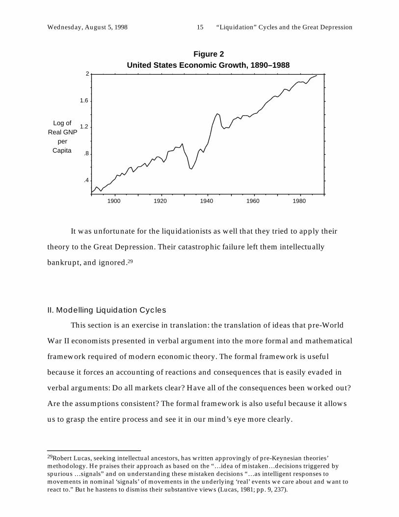
It was unfortunate for the economy that liquidationists were influential, and tried
to apply their theory to the Great Depression. It does not fit. Figure 2 plots the course of
real GNP per capita in the United States since 1890. Other recessions and depressions in
the figure might perhaps27 be interpreted as the process of liquidation of mistaken
investments that will inevitably take place in a dynamic economy under uncertainty,
The Great Depression is too large for such an interpretation to pass a minimal
plausibility test. During the Great Depression real national product per capita fell back
to its level of a quarter century before.28 The measured U.S. net real capita stock was the
same at the start of World War II as it had been in 1929.
27But I believe in most cases erroneously.28Note, however, that the extraordinary greatness of the Depression is a feature that became clear onlyafter World War II. Analysts in the middle of the Depression lacked the statistical information necessaryto accurately guage its quantitative pulse.
Wednesday, August 5, 1998 15 “Liquidation” Cycles and the Great Depression
.4
.8
1.2
1.6
2
1900 1920 1940 1960 1980
Log ofReal GNP
perCapita
Figure 2United States Economic Growth, 1890–1988
It was unfortunate for the liquidationists as well that they tried to apply their
theory to the Great Depression. Their catastrophic failure left them intellectually
bankrupt, and ignored.29
II. Modelling Liquidation Cycles
This section is an exercise in translation: the translation of ideas that pre-World
War II economists presented in verbal argument into the more formal and mathematical
framework required of modern economic theory. The formal framework is useful
because it forces an accounting of reactions and consequences that is easily evaded in
verbal arguments: Do all markets clear? Have all of the consequences been worked out?
Are the assumptions consistent? The formal framework is also useful because it allows
us to grasp the entire process and see it in our mind’s eye more clearly.
29Robert Lucas, seeking intellectual ancestors, has written approvingly of pre-Keynesian theories’methodology. He praises their approach as based on the “…idea of mistaken…decisions triggered byspurious …signals” and on understanding these mistaken decisions “…as intelligent responses tomovements in nominal ‘signals’ of movements in the underlying ‘real’ events we care about and want toreact to.” But he hastens to dismiss their substantive views (Lucas, 1981; pp. 9, 237).
Wednesday, August 5, 1998 16 “Liquidation” Cycles and the Great Depression
But Schumpeter was no model builder. Gaps must be filled in to raise the story as
told by Schumpeter to the level of consistency and formalization required of arguments
made by macroeconomists today. Translation inevitably produces shifts in meaning.
Translation into the language of modern economic theory is especially likely to do so.
Theory enforces a high degree of consistency and explicit formalization on arguments
made in it.
This section of this paper sketches a simple formal model of a “liquidationist”
cycle, in which an economy solving a dynamic social maximization problem—that is, an
economy that is doing the best that can be done at allocating scarce resources among
alternative uses—under uncertainty does at times find it optimal to “liquidate” capital,
enterprises, and sunk investments. Recessions do not arise because of avoidable
mistakes or ineffective policies, but because the future is uncertain and investors cannot
fully “pierce the veil of time and ignorance.” In this model business cycles cannot—as
Schumpeter said—be removed short of removing the dynamic element from economic
growth itself.
Note that the formal model presented below gives only a slice, and only a partial
slice, of liquidationist thought. It has only one sector, and so only one type of capital:
that portion of the “liquidationist” argument that hinges on the wrong kinds and not
just on too much capital being installed during boom years is suppressed. In addition,
modern economics frowns on interpretations that present groups of investors or
workers as making repeated patterns of mistakes.
Economists in the 1920’s were perfectly willing to argue that a given recession
had been generated by excessive and irrational overspeculation and overinvestment
during the previous boom: speculation had been irrational, and a recession was
required to work through the consequences. The recession cannot be avoided ex post,
given the excesses of the previous boom, even though it could have been avoided ex
ante, if the boom had been choked off when it began to be driven by irrational
overspeculation. But such an argument does not pass the standards required of
Wednesday, August 5, 1998 17 “Liquidation” Cycles and the Great Depression
economics today, and so the model presented below contains recessions that cannot be
avoided ex post and could not have been avoided ex ante because there was no reason at
the time to think that “overspeculation” was in progress. These are some of the shifts
produced by the process of translation.30
The model constructed here is by no means complete. It does not account for
why, released from the investment sector, productive resources are not employed in the
next day in the consumption goods sector, but instead remain idle and in “inventory”
for a time—that is presumably due to various market “frictions.”31 This section
presents only the accelerator portion of a liquidationist business cycle.
The Model
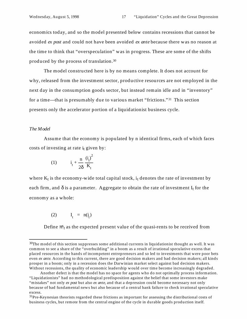
Assume that the economy is populated by n identical firms, each of which faces
costs of investing at rate it given by:
(1) it + 2δ
n
Kt
(it)2
where Kt is the economy-wide total capital stock, it denotes the rate of investment by
each firm, and δ is a parameter. Aggregate to obtain the rate of investment It for the
economy as a whole:
(2) It = n(it)
Define πst as the expected present value of the quasi-rents to be received from
30The model of this section suppresses some additional currents in liquidationist thought as well. It wascommon to see a share of the “overbuilding” in a boom as a result of irrational speculative excess thatplaced resources in the hands of incompetent entrepreneurs and so led to investments that were poor betseven ex ante. According to this current, there are good decision makers and bad decision makers; all kindsprosper in a boom; only in a recession does the Darwinian market select against bad decision makers.Without recessions, the quality of economic leadership would over time become increasingly degraded.
Another defect is that the model has no space for agents who do not optimally process information.“Liquidationists” had no methodological predisposition against the belief that some investors make“mistakes” not only ex post but also ex ante, and that a depression could become necessary not onlybecause of bad fundamental news but also because of a central bank failure to check irrational speculativeexcess.31Pre-Keynesian theorists regarded these frictions as important for assessing the distributional costs ofbusiness cycles, but remote from the central engine of the cycle in durable goods production itself.
Wednesday, August 5, 1998 18 “Liquidation” Cycles and the Great Depression
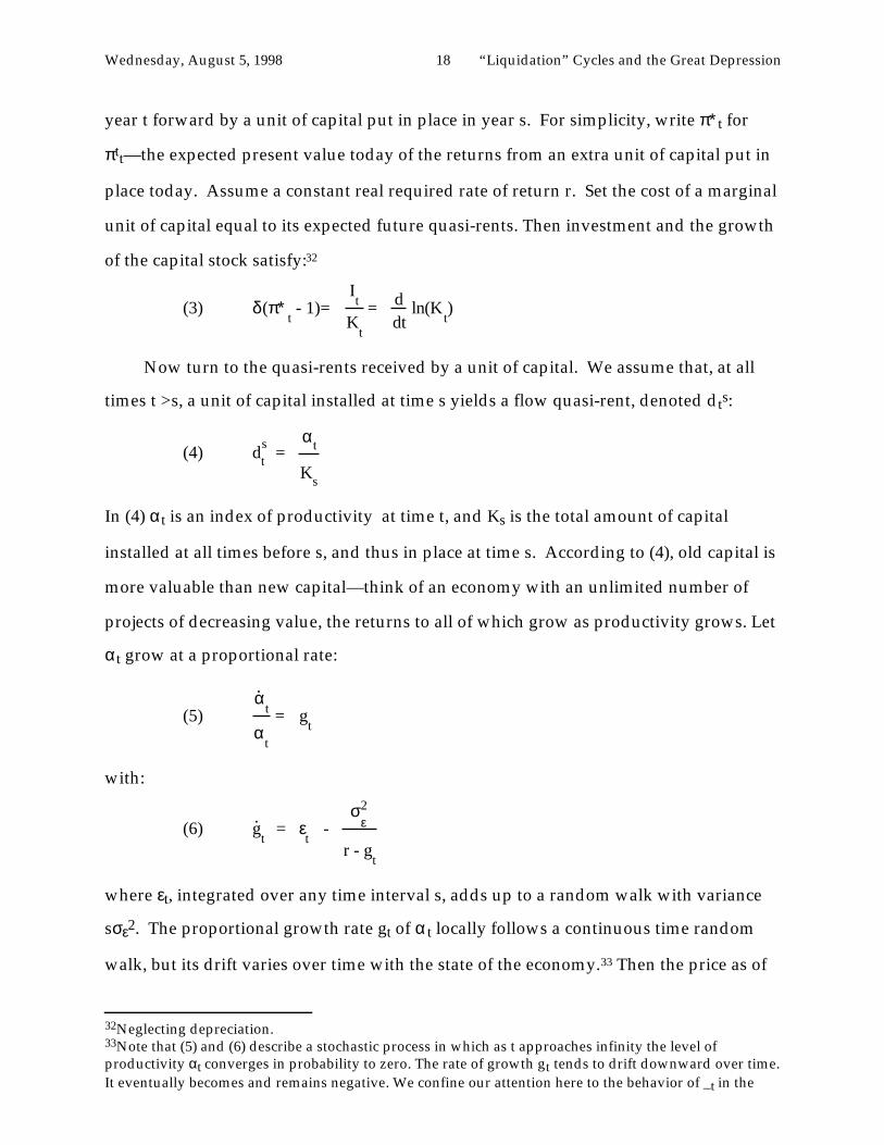
year t forward by a unit of capital put in place in year s. For simplicity, write π∗t for
πtt—the expected present value today of the returns from an extra unit of capital put in
place today. Assume a constant real required rate of return r. Set the cost of a marginal
unit of capital equal to its expected future quasi-rents. Then investment and the growth
of the capital stock satisfy:32
(3) δ(π∗t - 1)=
Kt
It =
dtd ln(K
t)
Now turn to the quasi-rents received by a unit of capital. We assume that, at all
times t >s, a unit of capital installed at time s yields a flow quasi-rent, denoted dts:
(4) dts
=Ks
αt
In (4) αt is an index of productivity at time t, and Ks is the total amount of capital
installed at all times before s, and thus in place at time s. According to (4), old capital is
more valuable than new capital—think of an economy with an unlimited number of
projects of decreasing value, the returns to all of which grow as productivity grows. Let
αt grow at a proportional rate:
(5)α
t
αt
= gt
.
with:
(6) gt
= εt -
r - gt
σε2
.
where εt, integrated over any time interval s, adds up to a random walk with variance
sσε2. The proportional growth rate gt of αt locally follows a continuous time random
walk, but its drift varies over time with the state of the economy.33 Then the price as of
32Neglecting depreciation.33Note that (5) and (6) describe a stochastic process in which as t approaches infinity the level ofproductivity αt converges in probability to zero. The rate of growth gt tends to drift downward over time.It eventually becomes and remains negative. We confine our attention here to the behavior of _t in the
Wednesday, August 5, 1998 19 “Liquidation” Cycles and the Great Depression
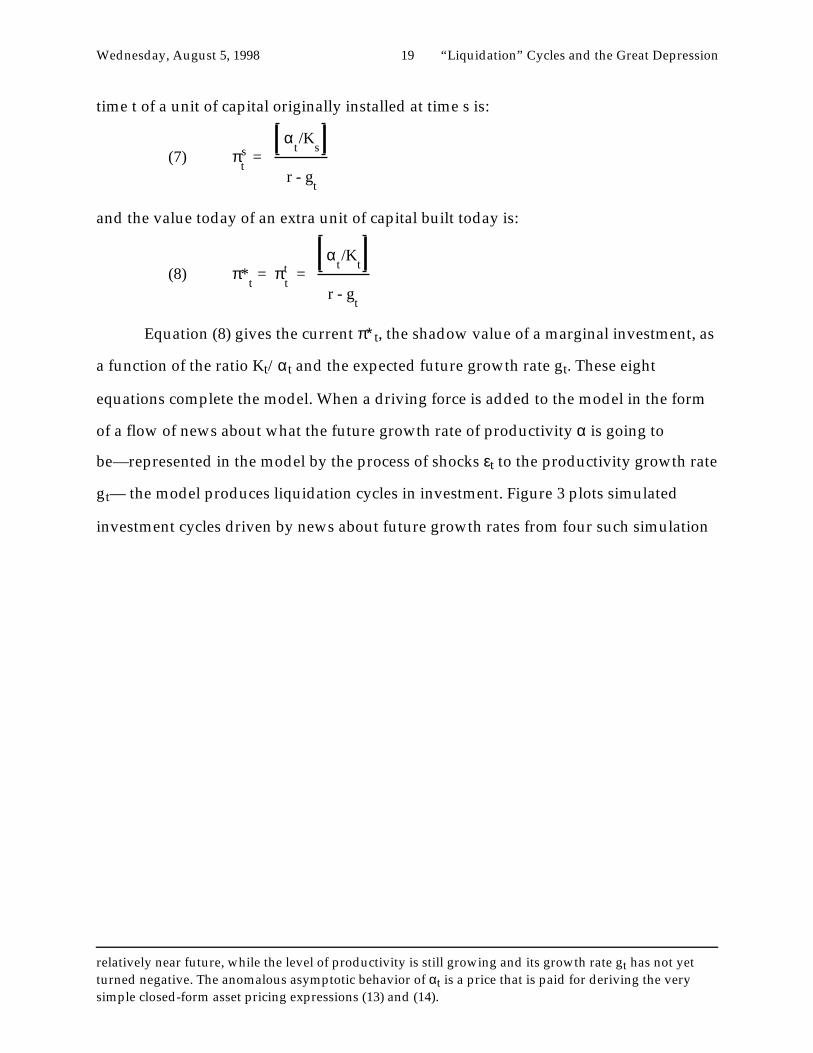
time t of a unit of capital originally installed at time s is:
(7) πts =
r - gt
αt/K
s
and the value today of an extra unit of capital built today is:
(8) π*t = π
tt =
r - gt
αt/K
t
Equation (8) gives the current π∗t, the shadow value of a marginal investment, as
a function of the ratio Kt/αt and the expected future growth rate gt. These eight
equations complete the model. When a driving force is added to the model in the form
of a flow of news about what the future growth rate of productivity α is going to
be—represented in the model by the process of shocks εt to the productivity growth rate
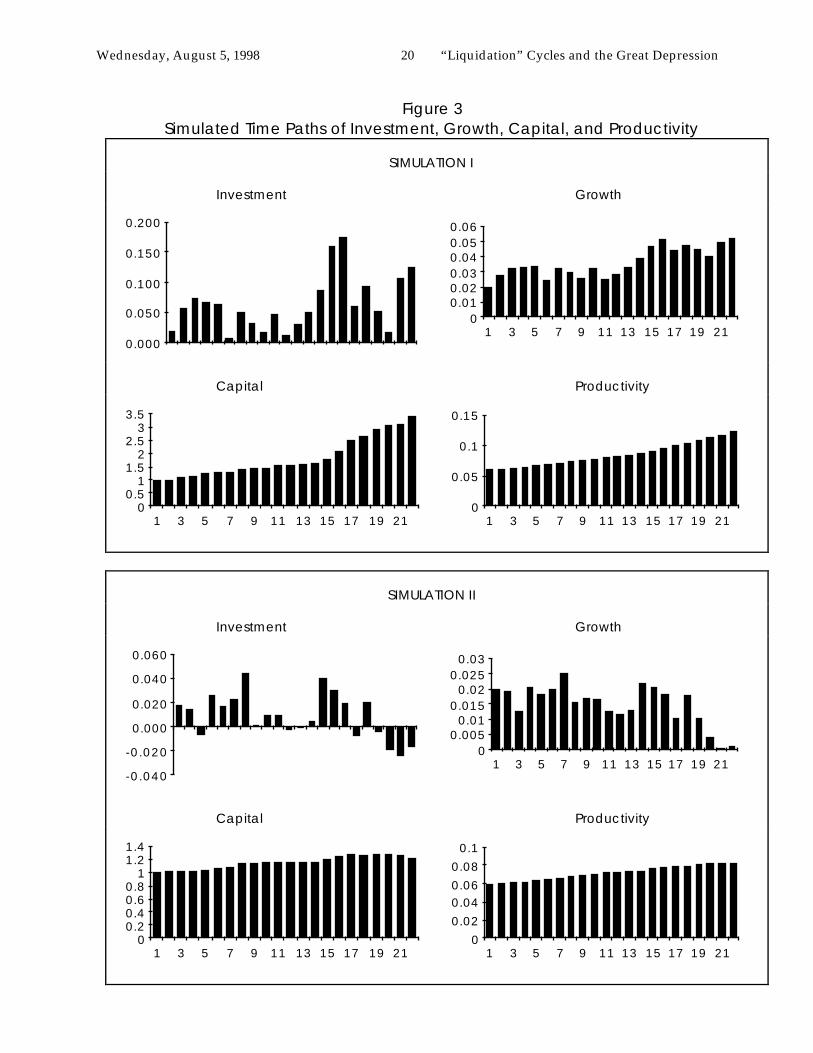
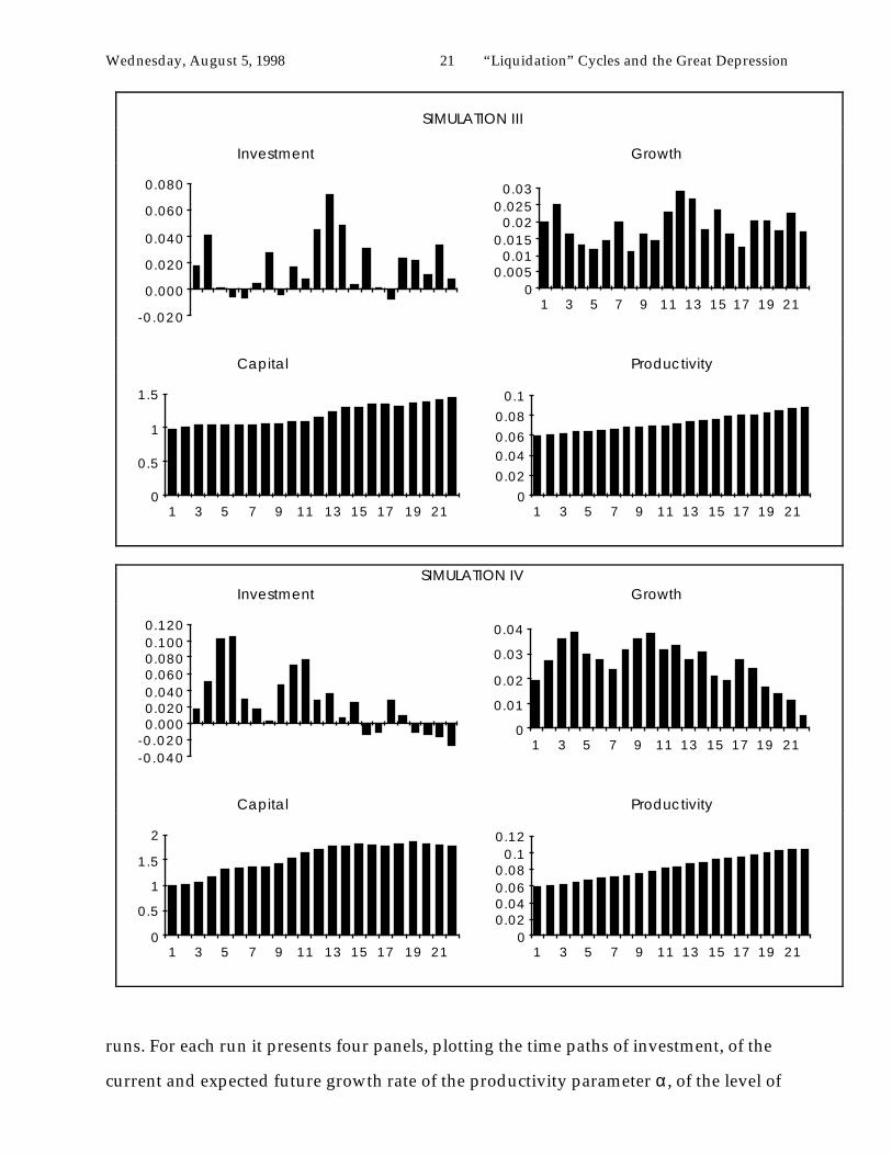
gt— the model produces liquidation cycles in investment. Figure 3 plots simulated
investment cycles driven by news about future growth rates from four such simulation
relatively near future, while the level of productivity is still growing and its growth rate gt has not yetturned negative. The anomalous asymptotic behavior of αt is a price that is paid for deriving the verysimple closed-form asset pricing expressions (13) and (14).
Wednesday, August 5, 1998 20 “Liquidation” Cycles and the Great Depression
Figure 3Simulated Time Paths of Investment, Growth, Capital, and Productivity
SIMULATION I
Investment Growth
0.000
0.050
0.100
0.150
0.200
00.010.020.030.040.050.06
1 3 5 7 9 11 13 15 17 19 21
Capital Productivity
00.5
11.5
22.5
33.5
1 3 5 7 9 11 13 15 17 19 210
0.05
0.1
0.15
1 3 5 7 9 11 13 15 17 19 21
SIMULATION II
Investment Growth
-0.040
-0.020
0.000
0.020
0.040
0.060
00.005
0.010.015
0.020.025
0.03
1 3 5 7 9 11 13 15 17 19 21
Capital Productivity
00.20.40.60.8
11.21.4
1 3 5 7 9 11 13 15 17 19 210
0.02
0.040.06
0.08
0.1
1 3 5 7 9 11 13 15 17 19 21
Wednesday, August 5, 1998 21 “Liquidation” Cycles and the Great Depression
SIMULATION III
Investment Growth
-0.020
0.000
0.020
0.040
0.060
0.080
00.005
0.010.015
0.020.025
0.03
1 3 5 7 9 11 13 15 17 19 21
Capital Productivity
0
0.5
1
1.5
1 3 5 7 9 11 13 15 17 19 210
0.02
0.040.06
0.08
0.1
1 3 5 7 9 11 13 15 17 19 21
SIMULATION IVInvestment Growth
-0.040-0.0200.0000.0200.0400.0600.0800.1000.120
0
0.01
0.02
0.03
0.04
1 3 5 7 9 11 13 15 17 19 21
Capital Productivity
0
0.5
1
1.5
2
1 3 5 7 9 11 13 15 17 19 210
0.020.040.060.08
0.10.12
1 3 5 7 9 11 13 15 17 19 21
runs. For each run it presents four panels, plotting the time paths of investment, of the
current and expected future growth rate of the productivity parameter α, of the level of
Wednesday, August 5, 1998 22 “Liquidation” Cycles and the Great Depression
the capital stock K, and of the level of the productivity parameter α.34
Figure 4 presents a schematic picture of why figure 3 shows times when
investment leaps ahead at a rapid pace, and times when investment stagnates or even
disinvestment occurs. Figure 4 graphs the K/α ratio on the horizontal axis, and the
current rate of new investment π on the vertical axis. The curve Π−Π shows, conditional
on the current expected rate of growth g, the relationship between the value of new
investment π and the K/α ratio given the expected growth rate g. The higher is K/α, the
higher the prospective profits from new investment and the higher is π., and so the Π−Π
curve slopes downward. The higher is g, the higher are the profits from new investment
and the higher is the Π−Π curve.
Let the economy begin at point A. Given the current growth rate g, the level of
the stock market is just high enough to keep the capital stock also growing at rate g and
so the ratio K/α constant. If there were no shocks to the rate of productivity growth, the
economy would remain at point A—with capital K and productivity α growing in
synchronization at a constant rate g—indefinitely.
Now suppose that there is bad news about future growth: g falls. Because of the
new, slower growth rate, the Π−Π curve shifts downward as well, to Π’−Π’. It is not that
present profits from new investments fall, but future profits are no longer expected to
grow as fast. The value of π drops instantly as the bad news spreads throughout
financial markets; the economy jumps instantly to point B in figure 4. If point B is
associated with a value of π less than one—if the fall to the Π’-Π’ curve is far
enough—absolute disinvestment will take place. In any event, a period of stagnant
investment or disinvestment and of a falling K/α ratio will follow as the economy
slowly moves up the Π’-Π’ curve to its new equilibrium at point C, at which the (lower)
pace of investment is just sufficient to keep the growth of capital K in step with the
(slower) growth of productivity α. A boom—a surge in investment following good
34Parameter values in the simulation runs are illustrative only: the discount rate r is set at 7.5%, theresponsiveness __of investment to shifts in π is set at 0.2, the initial rate of growth _0 of productivity is set
at 2% per period, and each period _ is subject to a random shock εt with standard deviation 0.6%.
Wednesday, August 5, 1998 23 “Liquidation” Cycles and the Great Depression
news about future productivity growth—would see the same process in reverse: a jump
upwards in π, a surge in investment, and then a move down the Π-Π curve to a new,
higher equilibrium value of K/α associated with the higher rate of productivity growth.
K/α
A
Figure 4 Response to Bad News About Future Productivity Growth
π
1C B
Π−ΠΠ’−Π’
old equilibrium value of πlower-growth equilibrium value of π
Figure 4 shows schematically the response to a single, once-and-for-all shock. But
actual economies see not one shock but a whole process as mixed good and bad news of
small and large magnitudes arrives in a constant flow. At times a flow of good news
about future growth—a series of positive ε shocks—leads to an investment boom, as
entrepreneurs hasten to put in place a large chunk of new capital that is expected to be
profitable given the future path of productivity that they forecast. And at times the
economy goes into depressions: the cumulative flow of news reveals that future growth
rates will be lower than expected—a series of ε shocks that add up to a negative
quantity—that capital has been overbuilt, and a substantial period of time will pass
during which it will be optimal for there to be no investment or disinvestment.
The underlying “fundamental” to which the capital stock is being adjusted in the
simulations of figure 3 is the level of the productive parameter α, which follows a
smooth path over time. There are substantial costs of adjusting the capital stock. Too
high a rate of investment or disinvestment in the short run quickly becomes very
expensive. Thus there are strong incentives to smooth out the path of investment over
Wednesday, August 5, 1998 24 “Liquidation” Cycles and the Great Depression
time. Yet even with all these sources of “smoothness” and gradual adjustment assumed
in the model, the time paths of investment generated in the simulation runs are sharp,
jagged, and variable.
These jagged paths are the best that can be done, given the rate at which news
about future productivity arrives.35 Because the future evolution of productivity is
unknown and the current capital stock is expensive to adjust means that the economy
will sometimes find that capital accumulation has fallen behind the ex post optimal pace,
and hasten to catch up by means of a boom, and will sometimes find that capital
accumulation has raced ahead of the pace that it turns out ex post would have been best,
and then hasten to liquidate and redeploy. If the future were known then investment
would follow a smooth and balanced-growth path. But in the environment of
uncertainty and lack of foresight assumed in the model, investment follows the jagged
path with irregular cycles simulated in figure 3.
Properly augmented by “frictions” that cause factors of production released from
the capital goods sector to spend time in “inventory” before they are reemployed in
other sectors, it could serve as a model of the business cycle.36 The “accelerator” above
provides a rationale for why reallocation of resources from consumption to investment
goods sectors and back again is a pervasive feature of business cycles. The economy,
maximizing a suitable objective function, must determine how much of its resources to
devote to capital accumulation without knowing what the long run productivity
growth rate will turn out to be ex post. The economy must guess; inevitably there will be
times it discovers that it has overestimated future growth. The subsequent process of
adjustment fis one of disinvestment and “liquidation.” Recognition that the future rate
of growth of technology will be slower carries with it a realization that there is an
35In a sense, this is the same point as that made by Kleidon (1986). Investment responds not tomovements in _ but to movements in the expected discounted value of all future α’s. Even though _ shiftsonly a small amount from period to period, the unstable nature of future productivity growth means thatthe expected discounted value of all future _’s shifts substantially.36One such account of how the reallocation of productive resources across sectors could lead tounemployment is given by Lilien (1982).
Wednesday, August 5, 1998 25 “Liquidation” Cycles and the Great Depression
“overhang” of capital, that old capital should be scrapped, and that new investment
projects should be postponed until this capital overhang has been absorbed.
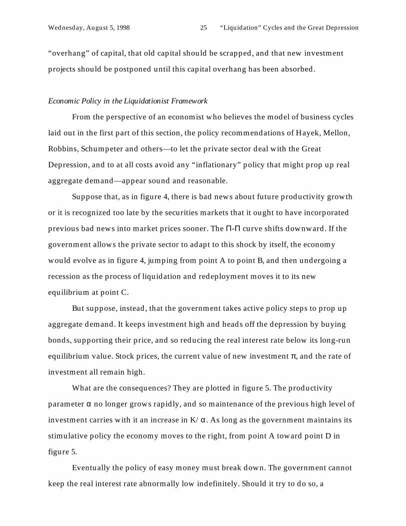
Economic Policy in the Liquidationist Framework
From the perspective of an economist who believes the model of business cycles
laid out in the first part of this section, the policy recommendations of Hayek, Mellon,
Robbins, Schumpeter and others—to let the private sector deal with the Great
Depression, and to at all costs avoid any “inflationary” policy that might prop up real
aggregate demand—appear sound and reasonable.
Suppose that, as in figure 4, there is bad news about future productivity growth
or it is recognized too late by the securities markets that it ought to have incorporated
previous bad news into market prices sooner. The Π-Π curve shifts downward. If the
government allows the private sector to adapt to this shock by itself, the economy
would evolve as in figure 4, jumping from point A to point B, and then undergoing a
recession as the process of liquidation and redeployment moves it to its new
equilibrium at point C.
But suppose, instead, that the government takes active policy steps to prop up
aggregate demand. It keeps investment high and heads off the depression by buying
bonds, supporting their price, and so reducing the real interest rate below its long-run
equilibrium value. Stock prices, the current value of new investment π , and the rate of
investment all remain high.
What are the consequences? They are plotted in figure 5. The productivity
parameter α no longer grows rapidly, and so maintenance of the previous high level of
investment carries with it an increase in K/α. As long as the government maintains its
stimulative policy the economy moves to the right, from point A toward point D in
figure 5.
Eventually the policy of easy money must break down. The government cannot
keep the real interest rate abnormally low indefinitely. Should it try to do so, a
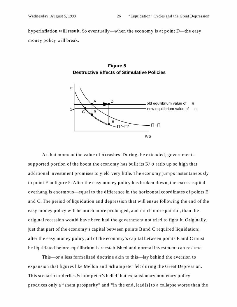
Wednesday, August 5, 1998 26 “Liquidation” Cycles and the Great Depression
hyperinflation will result. So eventually—when the economy is at point D—the easy
money policy will break.
K/α
A
Figure 5 Destructive Effects of Stimulative Policies
π
1C B
D
EΠ−ΠΠ’−Π’
old equilibrium value of πnew equilibrium value of π
At that moment the value of π crashes. During the extended, government-
supported portion of the boom the economy has built its K/α ratio up so high that
additional investment promises to yield very little. The economy jumps instantaneously
to point E in figure 5. After the easy money policy has broken down, the excess capital
overhang is enormous—equal to the difference in the horizontal coordinates of points E
and C. The period of liquidation and depression that will ensue following the end of the
easy money policy will be much more prolonged, and much more painful, than the
original recession would have been had the government not tried to fight it. Originally,
just that part of the economy’s capital between points B and C required liquidation;
after the easy money policy, all of the economy’s capital between points E and C must
be liquidated before equilibrium is reestablished and normal investment can resume.
This—or a less formalized doctrine akin to this—lay behind the aversion to
expansion that figures like Mellon and Schumpeter felt during the Great Depression.
This scenario underlies Schumpeter’s belief that expansionary monetary policy
produces only a “sham prosperity” and “in the end, lead[s] to a collapse worse than the
Wednesday, August 5, 1998 27 “Liquidation” Cycles and the Great Depression
one it was called in to remedy.”
The argument is logically consistent, once the premise about the nature of
depressions is accepted. But why were so many willing to accept the premise? Certainly
Keynes was not. He (1931; pp. 347–8) strongly argued that the boom of 1925–29 had not
produced an economy with an unsustainable or unbalanced capital structure:
While some part of the investment…was doubtless ill judged andunfruitful, there can…be no doubt that the world was enormouslyenriched by the constructions of …1925 to 1929; its wealthincreased in these five years by as much as in any other ten ortwenty years of its history.… [O]n the whole, I see little sign of anyserious want of balance such as is alleged by some authorities. Therates of growth [of different sectors]…seem to me…to have been inas good a balance as one could have expected.…A few morequinquennia of equal activity might, indeed, have brought us nearto the economic Eldorado where all our reasonable economic needswould be satisfied.
III. Sources of “Liquidationism”
Late-Nineteenth Century Railroad Cycles
One possible answer is that the “liquidationist” point of view had in fact been
correct in the past, or at least that it had not been grossly inconsistent with the business
cycles which Schumpeter and his colleagues had experienced in the generations before
World War I.
In countries that are undergoing rapid industrial revolutions and seeing rapid
increases in their capital/output ratios, swings in investment driven by news about
future growth may well be more important than in countries that have already
undergone industrial revolutions and attained relatively stable capital/output ratios. In
the U.S., the half century before World War II saw non-agricultural capital/output
ratios nearly double (Abramovitz and David, 1973). For half a century the pace,
direction, and completeness of U.S. industrialization was up for grabs: no one could
know ex ante how many railroad lines it would be worth building west of the
Wednesday, August 5, 1998 28 “Liquidation” Cycles and the Great Depression
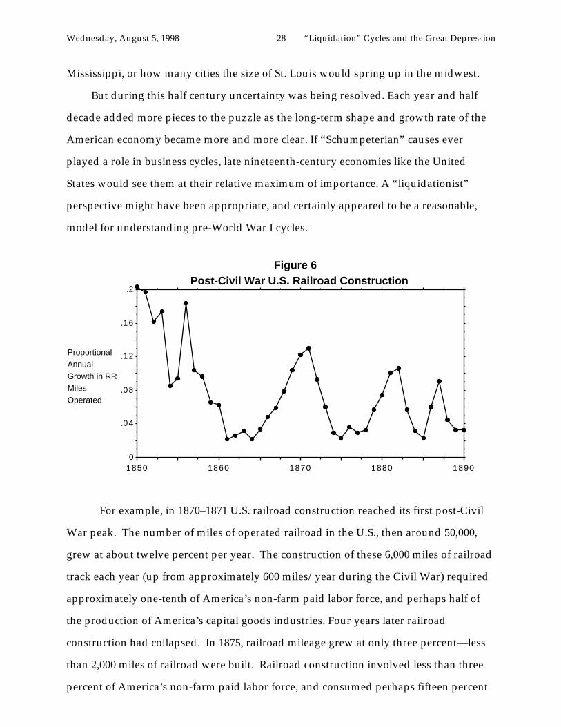
Mississippi, or how many cities the size of St. Louis would spring up in the midwest.
But during this half century uncertainty was being resolved. Each year and half
decade added more pieces to the puzzle as the long-term shape and growth rate of the
American economy became more and more clear. If “Schumpeterian” causes ever
played a role in business cycles, late nineteenth-century economies like the United
States would see them at their relative maximum of importance. A “liquidationist”
perspective might have been appropriate, and certainly appeared to be a reasonable,
model for understanding pre-World War I cycles.
0
.04
.08
.12
.16
.2
1850 1860 1870 1880 1890
Proportional Annual Growth in RR Miles Operated
Figure 6Post-Civil War U.S. Railroad Construction
For example, in 1870–1871 U.S. railroad construction reached its first post-Civil
War peak. The number of miles of operated railroad in the U.S., then around 50,000,
grew at about twelve percent per year. The construction of these 6,000 miles of railroad
track each year (up from approximately 600 miles/year during the Civil War) required
approximately one-tenth of America’s non-farm paid labor force, and perhaps half of
the production of America’s capital goods industries. Four years later railroad
construction had collapsed. In 1875, railroad mileage grew at only three percent—less
than 2,000 miles of railroad were built. Railroad construction involved less than three
percent of America’s non-farm paid labor force, and consumed perhaps fifteen percent
Wednesday, August 5, 1998 29 “Liquidation” Cycles and the Great Depression
of the potential production of America’s capital goods industries.
As figure 6 shows, two more substantial irregular waves of railroad building, one
peaking in 1881-1882 and a second peaking in 1887, passed through the economy before
1890. Each required an expansion of capacity in the railroad construction sector’s
suppliers—iron and steel for rails, timber for ties, mechanical equipment for
locomotives and cars, furniture to equip the Pullman Co. cars to carry passengers on the
new lines, and so forth—and a redirection of capacity from other industries and from
idle status to the production of railroad lines. Each wave also required the redirection
of perhaps one million workers to construction, and as the wave passed their
reallocation into other sectors or into relative idleness. These swings in railroad
construction, and the associated swings in total product, are what the pre-World War I
world saw as “business cycles.”
It is hard to interpret such late nineteenth-century railroad cycles as caused by
the forces to which business cycles are often attributed today. The small government
did not serve as a source of more than trivial fiscal shocks. There was no central bank to
mistakenly squeeze off economic activity by keeping the money supply from growing
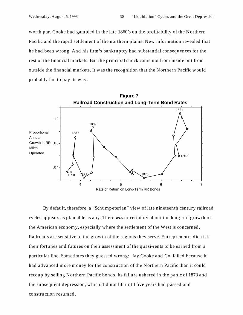
sufficiently rapidly.37 Indeed, the typical correlation over the 1870–1890 period goes the
wrong way: the post-1871 fall in railroad construction is associated not with rising but
with falling interest rates, as figure 7 shows.
It is difficult to attribute the railroad cycles to disturbances in financial markets.
The financing of railroads was the predominant business of financial markets, and
financial crises tended to result from downturns in railroad construction, not to cause
such downturns. In 1873 Jay Cooke and Co. went bankrupt because bond buyers no
longer believed that the northern tier of the great plains would be settled fast enough to
make the Northern Pacific Railroad a money-making bonanza and to make its bonds
37The international gold standard almost surely did play a role in causing some of U.S. business cycles.1893 and 1907 are prime candidates. But as Lewis (1978) shows, the business cycles in the industrial coreof the world economy did not move in synchronization in the half century before World War I. Eachcountry had its own internally-generated business cycle that was as if not more important in determiningoutput than the international transmission mechanism of the gold standard.
Wednesday, August 5, 1998 30 “Liquidation” Cycles and the Great Depression
worth par. Cooke had gambled in the late 1860’s on the profitability of the Northern
Pacific and the rapid settlement of the northern plains. New information revealed that
he had been wrong. And his firm’s bankruptcy had substantial consequences for the
rest of the financial markets. But the principal shock came not from inside but from
outside the financial markets. It was the recognition that the Northern Pacific would
probably fail to pay its way.
.04
.08
.12
4 5 6 7Rate of Return on Long-Term RR Bonds
Proportional Annual Growth in RR Miles Operated
1867
1871
1875
1882
1885
1887
1890
Figure 7Railroad Construction and Long-Term Bond Rates
By default, therefore, a “Schumpeterian” view of late nineteenth century railroad
cycles appears as plausible as any. There was uncertainty about the long run growth of
the American economy, especially where the settlement of the West is concerned.
Railroads are sensitive to the growth of the regions they serve. Entrepreneurs did risk
their fortunes and futures on their assessment of the quasi-rents to be earned from a
particular line. Sometimes they guessed wrong: Jay Cooke and Co. failed because it
had advanced more money for the construction of the Northern Pacific than it could
recoup by selling Northern Pacific bonds. Its failure ushered in the panic of 1873 and
the subsequent depression, which did not lift until five years had passed and
construction resumed.
Wednesday, August 5, 1998 31 “Liquidation” Cycles and the Great Depression
Thus railroad booms and busts of the late nineteenth century are not inconsistent
with a “liquidationist” perspective. When long run rates of growth are unstable,
investment for the future ought to be jagged, and ought to see periods of rapid
expansion coupled with periods of quiescence and disinvestment. This was
Schumpeter’s insight.38 It is a defensible view to take of the determinants of large
investment cycles in rapidly-growing economies like the United States in the second
half of the nineteenth century.
The claim made here is very limited. It is not that the “liquidationist” perspective
provides the correct interpretation of late nineteenth century railroad cycles. I would, in
fact, be somewhat surprised if this turned out to be the case. The claim is only that the
liquidationist perspective was not prima facie inconsistent with and could in fact provide
a natural explanation for nineteenth century railroad cycles.
In this context, it does not seem surprising that liquidationist theories became
popular around and after the turn of the twentieth century. They made apparent sense
of relatively recent historical experience. When the Great Depression came, theorists
like Robbins and Schumpeter tried to make sense of it in the same framework. With
hindsight we can see that the Depression was an order of magnitude larger than
previous depressions, that it was not a period of accelerated structural change, and that
as a result it is difficult to sustain an interpretation that sees it as necessary economic
housecleaning. Schumpeter and his school were working within a macroeconomic
framework that had once been reasonable, but had become inappropriate and proved
unhelpful in understanding and guiding policy during the Great Depression.
Implications
Getting the history of economic policy during the Great Depression right
38Blanchard, Rhee, and Summers (1990) find a strong relationship between the stock market andinvestment over the twentieth century. To the extent that the stock market and investment are respondingto the same factors and that large stock market swings are driven by shifting expectations of futuregrowth, there appears to be a possibility that “Schumpeterian” investment dynamics have played a rolein shaping the strength of business cycles, even if they have not determined their timing.
Wednesday, August 5, 1998 32 “Liquidation” Cycles and the Great Depression
requires an understanding of the hold exercised by the “liquidationist” perspective. The
Great Depression is a principal axis of twentieth century history. An astonishing feature
of the Depression, from our perspective, is the unwillingness of governments to take
steps to stimulate their economies during the slide of 1929–33. Advocates of the
“liquidationist” perspective argued that the Depression had come about because the
boom of the 1920’s had led to a capital overhang, and that investment could not proceed
until the productivity growth and depreciation had removed this excess past
investment. The policy recommendations of “liquidationists” were followed for much
of the Depression.
A large proportion of the capital stock was indeed liquidated. According to
Blanchard, Rhee, and Summers (1990), by 1936 all net capital accumulation over
1924–29 had been erased. Yet the years between 1936 and World War II did not see a
restoration of normal levels of activity and unemployment. This is a decisive
experiment: whatever caused the Depression and no matter how applicable
“liquidationist” theory may be to other episodes, the Depression was not caused by an
overhang of unproductive capital, for it outlasted any plausible such overhang.
It was, therefore, bad advice that academic economists like Robbins and
Schumpeter gave central banks and treasuries during the Depression. It is disturbing
that so many smart economists could give such destructive policy advice.
It is also disturbing that the advice they gave was not unreasonable, given the
business cycles that they had experienced. The market economy’s allocation of
resources between consumption and investment does involve the market’s solving a
dynamic problem in a stochastic environment. The arrival of news about future
productivities and opportunities does imply that there will be times at which new
information reveals that recent investments will not repay their costs. In such situations,
the correct policy is indeed to help the process of structural readjustment and
reallocation along, and not to delay reallocation by pumping up demand to freeze
production in its old pattern. To the extent that late nineteenth-century railroad cycles
Wednesday, August 5, 1998 33 “Liquidation” Cycles and the Great Depression
fit this pattern of speculation and overbuilding, it would have been counterproductive
from a long-run perspective for the government to try to keep railroad construction at a
high pace in a recession.
The advocates of the “liquidationist” point of view during the Great Depression
were mistaken, but not crazy. In many histories (Chandler, 1973; Galbraith, 1965), the
pronouncements of liquidationists appear to be incoherent barbarisms that were,
inexplicably, believed. Such interpretations get the history of economic thought wrong.
It is one thing to compare past barbarism to present enlightenment. It is another to
reflect that Robbins and Schumpeter were as smart and as hard working as anyone in
more recent generations—and were as sure that they knew the key to managing a fast-
growing market economy.
Wednesday, August 5, 1998 34 “Liquidation” Cycles and the Great Depression
References
Moses Abramovitz and Paul David (1973), “Reinterpreting American EconomicGrowth: Parables and Realities,” American Economic Review Papers and Proceedings 63(May), pp. 428–39.
Olivier Blanchard, Changyong Rhee, and Lawrence Summers (1990), “The Stock Marketand Investment.”
Douglass Brown et al. (1934), Economics of the Recovery Program (New York: McGraw-Hill).
E. Cary Brown (1956), “Fiscal Policy in the Thirties: A Reappraisal,” American EconomicReview 46 (December), pp. 857–79.
Karl Brunner and Allan Meltzer (1974) “Friedman’s Monetary Theory,” in Robert J.Gordon, ed., Milton Friedman’s Monetary Framework (Chicago, Il.: University ofChicago Press, 1974).
Lester Chandler (1970), America’s Greatest Depression (New York: Harper and Row).
J. Ronnie Davis (1971), The New Economics and the Old Economists (Ames, IO: Universityof Iowa Press).
Barry Eichengreen (1991), Golden Fetters: The Gold Standard and the Great Depression(forthcoming).
Gerald Epstein and Thomas Ferguson (1986), “Loan Liquidation…”
Milton Friedman and Anna J. Schwartz (1963), A Monetary History of the United States(Princeton, NJ: Princeton University Press).
Milton Friedman (1974), “Comments on the Critics,” in Robert J. Gordon, ed., MiltonFriedman’s Monetary Framework (Chicago, Il.: University of Chicago Press, 1974).
Milton Friedman (1984), “Monetary Policy for the 1980’s,” in John Moore, ed., ToPromote Prosperity (Palo Alto, CA: Hoover Institution).
John Kenneth Galbraith (1965), “How Keynes Came to America,” in John KennethGalbraith, Economics, Peace, and Laughter (Boston, Mass.: Houghton Mifflin, 1971).
Robert J. Gordon, ed. (1974), Milton Friedman’s Monetary Framework (Chicago, Il.:University of Chicago Press).
Peter A. Hall, ed. (1989), The Political Power of Economic Ideas: Keynesianism Across Nations(Princeton, N.J.: Princeton University Press).
Wednesday, August 5, 1998 35 “Liquidation” Cycles and the Great Depression
Robert Hall and John Taylor (????), Macroeconomics
Seymour Harris (1934), “Higher Prices,” in Douglass Brown et al., Economics of theRecovery Program (New York: McGraw-Hill, 1934).
Friedrich A. von Hayek (1944), The Road to Serfdom
Friedrich A. von Hayek (1935), Prices and Production (London: Routledge).
Friedrich A. von Hayek (1931), “The ‘Paradox’ of Saving,” Economica 32 (May), pp.125–69.
Herbert Hoover (1952), The Memoirs of Herbert Hoover (New York: Macmillan and Co.).
Harry Johnson (1969), “The Keynesian Revolution and the Monetarist Counter-Revolution,” in Harry Johnson and Elizabeth Johnson, In the Shadow of Keynes(Oxford: Basil Blackwell, 1978).
John Maynard Keynes (1931), “An Economic Analysis of Unemployment” (Universityof Chicago: 1931 Harris Foundation lectures); reprinted in John Maynard Keynes, TheGeneral Theory and After: Part I, Preparation, vol. XIII, pt. 1 of The Collected Writings ofJohn Maynard Keynes, Donald Moggridge, ed., (Cambridge, U.K.: CambridgeUniversity Press, 1972).
John Maynard Keynes (1936), The General Theory of Employment, Interest and Money(Cambridge, UK: Cambridge University Press).
Charles P. Kindleberger (1978), Manias, Panics, and Crashes (New York: Basic Books).
Allen Kleidon (1986), “Variance Bounds Tests and Stock Price Valuation Models,”Journal of Political Economy 94, pp. 953–1001.
W. Arthur Lewis (1978), Growth and Fluctuations (London: Allen and Unwin).
David Lilien (1982), “Sectoral Shifts and Unemployment,” Journal of Political Economy
Robert E. Lucas (1981), Studies in Business Cycle Theory (Cambridge, MA: M.I.T. Press).
Donald Patinkin (1982), Anticipations of the General Theory, and Other Essays on Keynes(Chicago, Il: University of Chicago Press).
Lionel Robbins (1935), The Great Depression (London: Macmillan).
Walter S. Salant (1989), “The Spread of Keynesian Doctrines and Practices in the UnitedStates,” in Peter A. Hall, ed., The Political Power of Economic Ideas: Keynesianism AcrossNations (Princeton, N.J.: Princeton University Press, 1989).
Paul Samuelson (1988), “The Role of Alvin Hansen in the Keynesian Revolution”
Wednesday, August 5, 1998 36 “Liquidation” Cycles and the Great Depression
(Cambridge, MA: M.I.T. xerox).
Joseph Schumpeter (1939), Business Cycles (New York: McGraw-Hill).
Joseph Schumpeter (1934), “Depressions,” in Douglass Brown et al., Economics of theRecovery Program (New York: McGraw-Hill, 1934).
Peter Temin (1989), Lessons from the Great Depression (Cambridge, MA: M.I.T. Press).
Peter Temin (1974), Did Monetary Forces Cause the Great Depression? (New York: W.W.Norton).
William Wiseley (1977), A Tool of Power: The Political History of Money (New York: JohnWiley).