Liquidity and Leverage

Hyun Song Shin (Princeton University) and Tobias Adrian (Federal Reserve Bank of New York)

Paper presented at the Financial Cycles, Liquidity, and Securitization Conference Hosted by the International Monetary Fund Washington, DC─April 18, 2008 The views expressed in this paper are those of the author(s) only, and the presence

of them, or of links to them, on the IMF website does not imply that the IMF, its Executive Board, or its management endorses or shares the views expressed in the paper.

FFIINNAANNCCIIAALL CCYYCCLLEESS,, LLIIQQUUIIDDIITTYY,, AANNDD SSEECCUURRIITTIIZZAATTIIOONNCCOONNFFEERREENNCCEE AAPPRRIILL 1188,, 22000088

Liquidity and Leverage�

Tobias Adrian

Federal Reserve Bank of New York

tobias.adrian@ny.frb.org

Hyun Song Shin

Princeton University

hsshin@princeton.edu

September 2007

Abstract

In a �nancial system where balance sheets are continuously marked tomarket, asset price changes show up immediately in changes in net worth,and elicit responses from �nancial intermediaries who adjust the size oftheir balance sheets. We document evidence that marked-to-market lever-age is strongly procyclical. Such behavior has aggregate consequences.Changes in aggregate balance sheets for intermediaries forecast changes inrisk appetite in �nancial markets, as measured by the innovations in theVIX index. Aggregate liquidity can be seen as the rate of change of theaggregate balance sheet of the �nancial intermediaries.

�A previous version of this paper was presented at the 6th BIS Annual Conference, \Finan-cial System and Macroeconomic Resilience", 18-19 June 2007 under its former title \Liquidityand Financial Cycles". We thank conference participants at the BIS conference, and seminarparticipants at the Federal Reserve Bank of New York, the Federal Reserve Bank of Chicago,and Princeton University for their comments. The views expressed in this paper are those ofthe authors and do not necessarily represent those of the Federal Reserve Bank of New York orthe Federal Reserve System.

1. Introduction

In a �nancial system where balance sheets are continuously marked to market,

changes in asset prices show up immediately on the balance sheet, and so have

an immediate impact on the net worth of all constituents of the �nancial system.

The net worth of �nancial intermediaries are especially sensitive to uctuations

in asset prices given the highly leveraged nature of such intermediaries' balance

sheets.

Our focus in this paper is on the reactions of the �nancial intermediaries to

changes in their net worth, and the market-wide consequences of such reactions.

If the �nancial intermediaries were passive and do not adjust their balance sheets

to changes in net worth, then leverage would fall when total assets rise. Change

in leverage and change in balance sheet size would then be negatively related.

However, as we will see below, the evidence points to a strongly positive re-

lationship between changes in leverage and changes in balance sheet size. Far

from being passive, the evidence points to �nancial intermediaries adjusting their

balance sheets actively, and doing so in such a way that leverage is high during

booms and low during busts. That is, leverage is procyclical.

Procyclical leverage can be seen as a consequence of the active management of

balance sheets by �nancial intermediaries who respond to changes in prices and

measured risk. For �nancial intermediaries, their models of risk and economic

capital dictate active management of their overall value at risk (VaR) through

adjustments of their balance sheets.

From the point of view of each �nancial intermediary, decision rules that result

in procyclical leverage are readily understandable. However, there are aggregate

consequences of such behavior for the �nancial system as a whole that are not

taken into consideration by an individual �nancial institution. We exhibit evidence

2

that procyclical leverage has spillover e�ects at the aggregate level through shifts

in risk appetite and funding liquidity. In particular, balance sheet uctuations

forecast shifts in risk appetite, as measured by the VIX index.

Our paper has two main objectives. Our �rst objective is to document the

determinants of balance sheet size and leverage for the group of �nancial interme-

diaries (including the major Wall Street investment banks) that operate primarily

through the capital markets. We show that leverage is strongly procyclical for

these intermediaries, and that the margin of adjustment on the balance sheet is

through repos and reverse repos (and other collateralized borrowing and lending).

In turn, procyclical leverage can be attributed to the bank's capital allocation

decision that rests on measured risks ruling at the time. We �nd that the value-

at-risk (VaR) disclosed by the banks is an important determinant of balance sheet

stance, but we also �nd evidence of an additional procyclical element in leverage

that operates over and above that implied by their disclosed value-at-risk.

Our second objective is to pursue the aggregate consequences of such procycli-

cal leverage, and document evidence that expansions and contractions of balance

sheets have important asset pricing consequences through shifts in market-wide

risk appetite. In particular, we show that changes in aggregate intermediary

balance sheet size can forecast innovations in market-wide risk premiums as mea-

sured by the VIX index of implied volatility in the stock market. We see this

as an important empirical �nding. Previous work in asset pricing has shown

that innovations in the VIX index capture key components of asset pricing that

conventional empirical models have been unable to address fully. By being able

to forecast shifts in risk appetite, we hope to inject a new element in thinking

about risk appetite and asset prices. The shift in risk appetite is closely related

to other notions of liquidity, such as the notion of \funding liquidity" used by

3

Brunnermeier and Pedersen (2005b)1. One of our contributions is to explain the

origins of funding liquidity in terms of �nancial intermediary behavior.

Our �ndings also shed light on the concept of \liquidity" as used in common

discourse about �nancial market conditions. In the �nancial press and other mar-

ket commentary, asset price booms are sometimes attributed to \excess liquidity"

in the �nancial system. Financial commentators are fond of using the associated

metaphors, such as the �nancial markets being \awash with liquidity", or liquidity

\sloshing around". However, the precise sense in which \liquidity" is being used

in such contexts is often left unspeci�ed.

Our empirical �ndings suggest that funding liquidity can be understood as the

rate of growth of aggregate balance sheets. When �nancial intermediaries' balance

sheets are generally strong, their leverage is too low. The �nancial intermediaries

hold surplus capital, and they will attempt to �nd ways in which they can employ

their surplus capital. In a loose analogy with manufacturing �rms, we may see

the �nancial system as having \surplus capacity". For such surplus capacity to be

utilized, the intermediaries must expand their balance sheets. On the liabilities

side, they take on more short-term debt. On the asset side, they search for

potential borrowers that they can lend to. Funding liquidity is intimately tied to

how hard the �nancial intermediaries search for borrowers.

The outline of our paper is as follows. We begin with a review of some very ba-

sic balance sheet arithmetic on the relationship between leverage and total assets.

The purpose of this initial exercise is to motivate our empirical investigation of the

balance sheet changes of �nancial intermediaries in section 3. Having outlined the

facts, in section 4, we show that changes in aggregate repo positions of the major

�nancial intermediaries can forecast innovations in the volatility risk-premium,

where the volatility risk premium is de�ned as the di�erence between the VIX

1See also Gromb and Vayanos (2002).

4

index and realized volatility. We conclude with discussions of the implications

of our �ndings for funding liquidity.

2. Some Basic Balance Sheet Arithmetic

What is the relationship between leverage and balance sheet size? We begin with

some very elementary balance sheet arithmetic, so as to focus ideas. Before look-

ing at the evidence for �nancial intermediaries, let us think about the relationship

between balance sheet size and leverage for a household. The household owns a

house �nanced with a mortgage. For concreteness, suppose the house is worth

100, the mortgage value is 90, and so the household has net worth (equity) of 10.

The initial balance sheet then is given by:

Assets Liabilities

100 1090

Leverage is de�ned as the ratio of total assets to equity, hence is 100=10 = 10.

What happens to leverage as total assets uctuate? Denote by A the market

value of total assets and E is the market value of equity. We make the simplifying

assumption that the market value of debt stays roughly constant at 90 for small

shifts in the value of total assets. Total leverage is then

L ' A

A� 90

Leverage is inversely related to total assets. When the price of my house goes up,

my net worth increases, and so my leverage goes down. Figure 2.1 illustrates the

negative relationship between total assets and leverage. Indeed, for households,

the negative relationship between total assets and leverage is clearly borne out

in the aggregate data. Figure 2.2 plots the quarterly changes in total assets to

quarterly changes in leverage as given in the Flow of Funds account for the United

5

Figure 2.1: Leverage for passive investor

States. The data are from 1963 to 2006. The scatter chart shows a strongly

negative relationship, as suggested by Figure 2.1.

Figure 2.2: Total Assets and Leverage of Household.

We can ask the same question for �rms, and we will address this question for

three di�erent types of �rms.

� Non-�nancial �rms

6

� Commercial banks

� Security brokers and dealers (including investment banks).

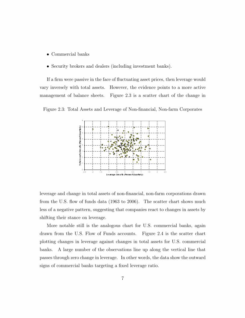
If a �rm were passive in the face of uctuating asset prices, then leverage would

vary inversely with total assets. However, the evidence points to a more active

management of balance sheets. Figure 2.3 is a scatter chart of the change in

Figure 2.3: Total Assets and Leverage of Non-�nancial, Non-farm Corporates

leverage and change in total assets of non-�nancial, non-farm corporations drawn

from the U.S. ow of funds data (1963 to 2006). The scatter chart shows much

less of a negative pattern, suggesting that companies react to changes in assets by

shifting their stance on leverage.

More notable still is the analogous chart for U.S. commercial banks, again

drawn from the U.S. Flow of Funds accounts. Figure 2.4 is the scatter chart

plotting changes in leverage against changes in total assets for U.S. commercial

banks. A large number of the observations line up along the vertical line that

passes through zero change in leverage. In other words, the data show the outward

signs of commercial banks targeting a �xed leverage ratio.

7

Figure 2.4: Total Assets and Leverage of Commercial Banks

However, even more striking than the scatter chart for commercial banks is that

for security dealers and brokers, that include the major Wall Street investment

banks. Figure 2.5 is the scatter chart for U.S. security dealers and brokers,

again drawn from the Flow of Funds accounts (1963 - 2006). The alignment of

the observations is now the reverse of that for households. There is a strongly

positive relationship between changes in total assets and changes in leverage. In

this sense, leverage is pro-cyclical.

In order to appreciate the aggregate consequences of pro-cyclical leverage, let

us �rst consider the behavior of a �nancial intermediary that manages its balance

sheet actively to as to maintain a constant leverage ratio of 10. Suppose the

initial balance sheet is as follows. The �nancial intermediary holds 100 worth of

securities, and has funded this holding with debt worth 90.

Assets Liabilities

Securities, 100 Equity, 10Debt, 90

8

Figure 2.5: Total Assets and Leverage of Security Brokers and Dealers

Assume that the price of debt is approximately constant for small changes in

total assets. Suppose the price of securities increases by 1% to 101.

Assets Liabilities

Securities, 101 Equity, 11Debt, 90

Leverage then falls to 101=11 = 9:18. If the bank targets leverage of 10, then

it must take on additional debt of D to purchase D worth of securities on the

asset side so thatassets

equity=101 +D

11= 10

The solution is D = 9. The bank takes on additional debt worth 9, and

with this money purchases securities worth 9. Thus, an increase in the price of

the security of 1 leads to an increased holding worth 9. The demand curve is

upward-sloping. After the purchase, leverage is now back up to 10.

9

Assets Liabilities

Securities, 110 Equity, 11Debt, 99

The mechanism works in reverse, too. Suppose there is shock to the securities

price so that the value of security holdings falls to 109. On the liabilities side,

it is equity that bears the burden of adjustment, since the value of debt stays

approximately constant.

Assets Liabilities

Securities, 109 Equity, 10Debt, 99

Leverage is now too high (109=10 = 10:9). The bank can adjust down its

leverage by selling securities worth 9, and paying down 9 worth of debt. Thus, a

fall in the price of securities of leads to sales of securities. The supply curve is

downward -sloping. The new balance sheet then looks as follows.

Assets Liabilities

Securities, 100 Equity, 10Debt, 90

The balance sheet is now back to where it started before the price changes.

Leverage is back down to the target level of 10.

Leverage targeting entails upward-sloping demands and downward-sloping sup-

plies. The perverse nature of the demand and supply curves are even stronger

when the leverage of the �nancial intermediary is pro-cyclical - that is, when

leverage is high during booms and low during busts. When the securities price

10

Figure 2.6: Adjustment of Leverage in Booms

goes up, the upward adjustment of leverage entails purchases of securities that

are even larger than that for the case of constant leverage. If, in addition, there

is the possibility of feedback, then the adjustment of leverage and price changes

will reinforce each other in an ampli�cation of the �nancial cycle.

If we hypothesize that greater demand for the asset tends to put upward pres-

sure on its price (a plausible hypothesis, it would seem), then there is the potential

for a feedback e�ect in which stronger balance sheets feed greater demand for the

asset, which in turn raises the asset's price and lead to stronger balance sheets.

Figure 2.6 illustrates the feedback during a boom. The mechanism works exactly

in reverse in downturns. If we hypothesize that greater supply of the asset tends

to put downward pressure on its price, then there is the potential for a feedback

e�ect in which weaker balance sheets lead to greater sales of the asset, which

depresses the asset's price and lead to even weaker balance sheets. Figure 2.7

illustrates the feedback during a downturn.

In section 4, we return to the issue of feedback by exhibiting evidence that

is consistent with the ampli�cation e�ects sketched above. We will see that

11

Figure 2.7: Leverage Adjustment in Downturn

changes in key balance sheet components forecast changes in the VIX index of

implied volatility in the stock market.

3. A First Look at the Evidence

3.1. Investment Bank Balance Sheets

To set the stage for our empirical study, we begin by examining the quarterly

changes in the balance sheets of �ve large investment banks, as listed below in

Table 1. The data are drawn from the Mergent database, which in turn are based

on the regulatory �lings with the U.S. Securities and Exchange Commission (SEC)

on their 10-K and 10-Q forms.

Table 1: Investment Banks

12

Name SampleBear Stearns 1997 Q1 { 2007 Q1

Goldman Sachs 1999 Q2 { 2007 Q1Lehman Brothers 1993 Q2 { 2007 Q1

Merrill Lynch 1991 Q1 { 2007 Q1Morgan Stanley 1997 Q2 { 2007 Q1

Our choice of these �ve banks is motivated by our concern to examine \pure

play" investment banks that are not part of a larger commercial banking group so

as to focus attention on their behavior with respect to the capital markets2. Cit-

igroup reported its investment banking operations separately from its commercial

banking operations until 2004 as \Citigroup Global Markets", and we have data

for the period 1998Q1 to 2004Q4. In some of our charts below, we will report

Citigroup Global Markets for comparison for reference. The stylized balance

sheet of an investment bank is as follows.

Assets Liabilities

Trading assets Short positionsReverse repos ReposOther assets Long term debt

Shareholder equity

On the asset side, traded assets are valued at market prices or are short term

collateralized loans (such as reverse repos) for which the discrepancy between face

value and market value are very small due to the very short term nature of the

loans. On the liabilities side, short positions are at market values, and repos

are very short term borrowing. We will return to a more detailed descriptions

of repos and reverse repos below. Long-term debt is typically a very small frac-

tion of the balance sheet.3 For these reasons, investment banks provide a good

2Hence, we do not include JP Morgan Chase, Credit Suisse, Deutsche Bank, and otherbrokerage operations that are part of a larger commercial bank.

3The balance sheet of Lehman Brothers as of November 2005 shows that short positions arearound a quarter of total assets, and long term debt is an even smaller fraction. Shareholder

13

approximation of the balance sheet that is continuously marked to market, and

hence provide insights into how leverage changes with balance sheet size.

The second reason for our study of investment banks lies in their continuously

increasing signi�cance for the �nancial system.

Figure 3.1:

Figure 3.1 plots the size of securities �rms' balance sheets relative to that

of commercial banks. We also plot the assets under management for hedge

funds, although we should be mindful that \assets under management" refers to

total shareholder equity, rather than the size of the balance sheet. To obtain

total balance sheet size, we should multiply by leverage. Figure 3.1 shows that

when expressed as a proportion of commercial banks' balance sheets, securities

�rms have been increasing their balance sheets at a very rapid rate. Note that

when hedge funds' assets under management is converted to balance sheet size by

multiplying by a conservative leverage factor of 2, the combined balance sheets

equity is around 4% of total assets (implying leverage of around 25). Short-term borrowing interms of repurchase agreements and other collateralized borrowing takes up the remainder.

14

of investment banks and hedge funds is over 50% of commercial banks balance

sheets.

Size is not the only issue. When balance sheets are marked to market, the

responses to price changes may entail responses that may be disproportionately

large. LTCM's balance sheet was small relative to the total �nancial sector,

but its impact would have been underestimated if only size had been taken into

account. Similarly, the size of the sub-prime mortgage exposures was small

relative to the liabilities of the �nancial system as a whole, but the credit crisis

of 2007 demonstrates that its impact can be large. Table 2 gives the summary

statistics of the investment banks over the sample period.

[Table 2]

We begin with the key question left hanging from the previous section. What

is the relationship between leverage and total assets? The answer is provided in

the scatter charts in �gure 3.3. We have included the scatter chart for Citigroup

Global Markets (1998Q1 - 2004Q4) for comparison, although Citigroup does not

�gure in the panel regressions reported below. The scatter chart shows the growth

in assets and leverage at a quarterly frequency. In all cases, leverage is large when

total assets are large. Leverage is pro-cyclical.

There are some notable common patterns in the scatter charts, but also some

notable di�erences. The events of 1998 are clearly evident in the scatter charts.

The early part of the year saw strong growth in total assets, with the attendant

increase in leverage. However, the third and fourth quarters of 1998 shows all

the hallmarks of �nancial distress and the attendant retrenchment in the balance

sheet. For most banks, there were very large contractions in balance sheet size in

1998Q4, accompanied by large falls in leverage. These points are on the bottom

left hand corners of the respective scatter charts, showing large contractions in

15

Figure 3.2:

Figure 3.3:

16

the balance sheet and decrease in leverage. Lehman Brothers and Merrill Lynch

seem especially hard hit in 1998Q4.

However, there are also some notable di�erences. It is notable, for instance,

that for Citigroup Global Markets, the large retrenchment seems to have happened

in the third quarter of 1998, rather than in the �nal quarter of 1998. Such a

retrenchment would be consistent with the closing down of the former Salomon

Brothers �xed income arbitrage desk on July 6th 1998 following the acquisition

of the operation by Travelers Group (later, Citigroup). Many commentators see

this event as the catalyst for the sequence of events that eventually led to the

demise of Long Term Capital Management (LTCM) and the associated �nancial

distress in the summer and early autumn of 1998.4

[Table 3]

Table 3 shows the results of a panel regression for change in leverage. The

negative relationship between the change in leverage and change in total assets is

con�rmed in the �nal column (column (v)) of Table 3. The coe�cient on lagged

leverage (i.e. previous quarter's leverage) is negative, suggesting that there is

mean-reversion in the leverage ratio for the banks. Leverage is positively related

to repos.

More interestingly, the regressions reveal which items on the balance sheet are

adjusting when balance sheets expand and contract. In particular, the regressions

show that the margin of adjustment in the expansion and contraction of balance

sheets is through repos. In a repurchase agreement (repo), an institution sells a

security while simultaneously agreeing to buy it back at a pre-agreed price on a

�xed future date. Such an agreement is tantamount to a collateralized loan, with

4The o�cial account (BIS, 1999) is given in the report of the CGFS of the Bank for Inter-national Settlements (the so-called \Johnson Report"). Popular accounts, such as Lowenstein(2000) give a description of the background and personalities.

17

the interest on the loan being the excess of the repurchase price over the sale price.

From the perspective of the funds lender { the party who buys the security with

the undertaking to re-sell it later { such agreements are called reverse repos. For

the buyer, the transaction is equivalent to granting a loan, secured on collateral.

Repos and reverse repos are important �nancing activities that provide the

funds and securities needed by investment banks to take positions in �nancial

markets. For example, a bank taking a long position by buying a security needs

to deliver funds to the seller when the security is received on settlement day. If

the dealer does not fully �nance the security out of its own capital, then it needs

to borrow funds. The purchased security is typically used as collateral for the

cash borrowing. When the bank sells the security, the sale proceeds can be used

to repay the lender.

Reverse repos are loans made by the investment bank against collateral. The

bank's prime brokerage business vis-�a-vis hedge funds will �gure prominently in

the reverse repo numbers. The scatter chart gives a glimpse into the way in

which changes in leverage are achieved through expansions and contractions in

the collateralized borrowing and lending. We saw in our illustrative section on

the elementary balance sheet arithmetic that when a bank wishes to expand its

balance sheet, it takes on additional debt, and with the proceeds of this borrowing

takes on more assets.

Figure 3.4 plots the change in assets against change in collateralized borrowing.

The positive relationship in the scatter plot con�rms our panel regression �nding

that balance sheet changes are accompanied by changes in short term borrowing.

Figure 3.5 plots the change in repos against the change in reverse repos. A

dealer taking a short position by selling a security it does not own needs to deliver

the security to the buyer on the settlement date. This can be done by borrowing

18

Figure 3.4:

19

Figure 3.5:

20

the needed security, and providing cash or other securities as collateral. When the

dealer closes out the short position by buying the security, the borrowed security

can be returned to the securities lender. The scatter plot in �gure 3.5 suggests

that repos and reverse repos play such a role as counterparts in the balance sheet.

3.2. Value at Risk

Procyclical leverage is not a term that the banks themselves are likely to use in

describing what they do, although this is in fact what they are doing. To get a

better handle on what motivates the banks in their actions, we explore the role of

value at risk (VaR) in explaining the banks' balance sheet decisions.

For a random variable A, the value at risk at con�dence level c relative to

some base level A0 is de�ned as the smallest non-negative number V aR such that

Prob (A < A0 � V aR) � 1� c

For instance, A could be the total marked-to-market assets of the �rm at some

given time horizon. Then the value at risk is the equity capital that the �rm must

hold in order to stay solvent with probability c. Financial intermediaries publish

their value at risk numbers as part of their regulatory �lings, and also regularly

disclose such numbers through their annual reports. Their economic capital is

tied to the overall value at risk of the whole �rm, where the con�dence level is set

at a level high enough to target a given credit rating (typically A or AA).

If �nancial intermediaries adjust their balance sheets to target a ratio of Value-

at-Risk to economic capital, then we may conjecture that their disclosed Value-

at-Risk �gures would be informative in reconstructing their actions. If the bank

maintains capital K to meet total value at risk, then we have

K = �� V aR (3.1)

21

where � is the proportion of capital that the intermediary holds per unit of V aR.

The proportionality � is potentially time varying. Hence, leverage L satis�es

L =A

K=1

�� A

V aR

Procyclical leverage then translates directly to counter -cyclical nature of unit

value-at-risk (i.e. value-at-risk per dollar of assets). Measured risk is low during

booms and high during busts. We can indeed see this counter-cyclical relationship

in the data. In Figure 3.6, we plot the VaR to total asset ratio against total assets

and see that it is downwardsloping (we have removed �xed e�ects to produce this

plot).

We explore the way in which the ratio of total value at risk to equity varies

over time. Equation (3.1) suggests that it would be informative to track the ratio

of value at risk to shareholder equity over time. The naive hypothesis would

be that this ratio is kept constant over time by the bank. The naive hypothesis

also ties in neatly the regulatory capital requirements under the 1996 Market Risk

Amendment of the Basel capital accord. Under this rule, the regulatory capital

is 3 times the 10 day, 99% value at risk. If total value risk is homogenous of

degree 1, then (3.1) also describes the required capital for the bank, also.

In Figure 3.7 we plot the evolution of the VaR/equity ratio and leverage over

time. We can see that both ratio are fairly constant. Only Goldman Sachs exhibits

a marked increase in leverage (and a corresponding increase in VaR/Equity) over

time. On average, both leverage and VaR/equity appear stationary, which is in

accordance with the risk management and regulatory constraints.

Table 4 presents the regressions for the quarterly change in the ratio of value at

risk to equity. Value at risk numbers are those numbers that the banks themselves

have reported in their 10-K and 10-Q �lings. For the reasons outlined already,

the �rm's self-assessed value at risk is closely tied to its assessment of economic

22

Figure 3.6:

23

Figure 3.7:

24

capital, and we would expect behavior to be heavily in uenced by changes in value

at risk.

[Table 4]

We focus on the ratio of value at risk to equity. In the panel regressions, the

lagged value at risk to equity ratio is strongly negative, with coe�cients in the

range of �0:5 to �0:6, suggesting rapid reversion to the mean. We take this as

evidence that the banks use VaR as a cue for how they adjust their balance sheets.

However, the naive hypothesis that banks maintain a �xed ratio of value at risk to

equity does not seem to be supported in the data. Column (ii) of Table 4 suggests

that an increase in the value at risk to equity ratio coincides with periods when the

bank increases its leverage. Value at risk to equity is procyclical, when measured

relative to leverage. However, total assets have a negative sign in column (v). It

appears that value at risk to equity is procyclical, but total assets adjust down

some of the e�ects captured in leverage. The evidence points to an additional,

procyclical risk appetite component to banks' exposures that goes beyond the

simple hypothesis of targeting a normalized value at risk measure.

4. Forecasting Risk Appetite

We now present the main results of our paper. We show the asset pricing conse-

quences of balance sheet expansion and contraction. We have already noted how

the demand and supply responses to price changes can become perverse when

�nancial intermediaries' actions result leverage that co-vary positively with the

�nancial cycle. We exhibit empirical evidence that the waxing and waning of

balance sheets have a direct impact on asset prices through the ease with which

traders, hedge funds and other users of credit can obtain funding for trades.

25

So far, we have used quarterly data drawn either from the balance sheets

of individual �nancial intermediaries or the aggregate balance sheet items from

the Flow of Funds accounts. However, for the purpose of tracking the �nancial

market consequences of balance sheet adjustments, data at a higher frequency is

more likely to be useful. For this reason, we use the weekly data on the primary

dealer repo and reverse repo positions compiled by the Federal Reserve Bank of

New York.

Primary dealers are the dealers with whom the Federal Reserve has an on-going

trading relationship in the course of daily business. The Federal Reserve collects

data that cover transactions, positions, �nancing, and settlement activities in U.S.

Treasury securities, agency debt securities, mortgage-backed securities (MBS),

and corporate debt securities for the primary dealers. The data are used by the Fed

to monitor dealer performance and market conditions, and are also consolidated

and released publicly on the Federal Reserve Bank of New York website5. The

dealers supply market information to the Fed as one of several responsibilities to

maintain their primary dealer designation and hence their trading relationship

with the Fed. It is worth noting that the dealers comprise an important but

limited subset of the overall market. Moreover, dealer reporting entities may not

re ect all positions of the larger organizations. Nevertheless, the primary dealer

data provide a valuable window on the overall market, at a frequency (every week)

that is much higher than the usual quarterly reporting cycle.

Dealers gather information at the close of business each Wednesday, on their

transactions, positions, �nancing, and settlement activities over the previous week.

They report on U.S. Treasury securities, agency debt securities, mortgage backed

securities, and corporate debt securities. Data are then submitted on the following

day (that is, Thursday) via the Federal Reserve System's Internet Electronic Sub-

5www.newyorkfed.org/markets/primarydealers.html

26

mission System. Summary data are released publicly by the Fed each Thursday,

one week after they are collected. The data are aggregated across all dealers, and

are only available by asset class (that is, Treasuries, agencies, etc.). Individual

issue data, and individual dealer data, are not released publicly.

Repos and reverse repos are an important subset of the security �nancing data.

The �nancing is reported on a gross basis, distinguishing between \securities in"

and \securities out" for each asset class. \Securities in" refer to securities received

by a dealer in a �nancing arrangement (be it against other securities or cash),

whereas \securities out" refer to securities delivered by a dealer in a �nancing

arrangement (be it against securities or cash). For example, if a dealer enters into

a repo, in which it borrows funds and provides securities as collateral, it would

report securities out. Repos and reverse repos are reported across all sectors. The

actual �nancing numbers reported are the funds paid or received. In the case of a

repo, for example, a dealer reports the actual funds received on the settlement of

the starting leg of the repo, and not the value of the pledged securities. In cases

where only securities are exchanged, the market value of the pledged securities is

reported.

[Table 5]

We use the weekly repo and reverse repo data to forecast �nancial market

conditions in the following week. Summary statistics are in Table 5. Our

measure of �nancial market conditions is the VIX index of the weighted average

of the implied volatility in the S&P500 index options. The VIX index has found

widespread application in empirical work as a proxy for market risk appetite.

Ang, Hodrick, Xing, and Zhang (2006) show that VIX innovations are signi�cant

pricing factors for the cross section of equity returns, and Bollerslev and Zhou

(2007) show that the volatility risk premium |the di�erence between the VIX

27

and realized volatility of the S&P500 index | forecasts equity returns better

than other commonly used forecasting variables (such as the P/E ratio or the

term spread).

We use the daily VIX data from the website of the Chicago Board Options

Exchange (www.cboe.com/micro/vix), and compute the S&P500 volatility from

daily data over weekly windows. We compute the volatility risk premium as

the di�erence between implied volatility and realized volatility. This risk pre-

mium is closely linked to the payo� to volatility swaps, which are zero investment

derivatives that return the di�erence between realized future volatility and implied

volatility over the maturity of the swap (see Carr and Wu (2007) for an analysis

of variance and volatility swaps). We then compute averages of the VIX and the

variance risk premium over each week (from the close of Wednesday to the close

of the following Tuesday).

We are able to forecast innovations in the VIX. This can be seen in columns

(ii)-(vi) of Table 6. We report forecasting regressions for VIX changes over the

next week, as well as the Wednesday-Thursday and Wednesday-Friday changes.

All of the forecasting results are signi�cant at the 1% level. The forecasting R2

increases from 8.9% when only the past VIX level is used, column (i) to 11.6%

when Repo changes are included in the forecast. We believe the latter result (the

ability to forecast the innovation in implied volatility) to be a very signi�cant

result. The forecasting result also holds for reverse repos, consistent with the

notion that it is the total size of the balance sheet that matters for aggregate

liquidity.

[Table 6]

In order to gain a better understanding what is determining the forecasting

result, we also run the forecasting regressions for S&P500 volatility and the volatil-

28

Figure 4.1:

ity risk premium (columns vii-x). We see that it is the volatility risk premium

that is being forecast, not actual equity volatility. Adjustments to the size of

�nancial intermediary balance sheets via repos thus forecasts the price of risk of

aggregate volatility, rather than aggregate volatility itself. We provide a graphical

illustration of the forecasting power of repos in Figure 4.1.

We can put forward the following economic rationale for the forecasting re-

gressions presented here. When balance sheets expand through the increased

collateralized lending and borrowing by �nancial intermediaries, the newly re-

29

leased funding resources then chase available assets for purchase. More capital

is deployed in increasing trading positions through the chasing of yield, and the

selling of the \tails", as in the selling of out of the money puts. If the increased

funding for asset purchases result in the generalized increase in prices and risk

appetite in the �nancial system, then the expansion of balance sheets will even-

tually be re ected in the asset price changes in the �nancial system - hence, the

ability of changes in repo positions to forecast future risk appetite.

5. Related Literature

The targeting of leverage seems closely to the bank's attempt to target a particular

credit rating. To the extent that the \passive" credit rating should uctuate

with the �nancial cycle, the fact that a bank's credit rating remains constant

through the cycle suggests that banks manage their leverage actively, so as to shed

exposures during downturns. Kashyap and Stein (2003) draw implications from

such behavior for the pro-cyclical impact of the Basel II bank capital requirements.

To the extent that balance sheets play a central role in our paper, our discussion

here is related to the large literature on the ampli�cation of �nancial shocks. The

literature has distinguished two distinct channels. The �rst is the increased credit

that operates through the borrower's balance sheet, where increased lending comes

from the greater creditworthiness of the borrower (Bernanke and Gertler (1989),

Kiyotaki and Moore (1998, 2001)). The second is the channel that operates

through the banks' balance sheets, either through the liquidity structure of the

banks' balance sheets (Bernanke and Blinder (1988), Kashyap and Stein (2000)),

or the cushioning e�ect of the banks' capital (Van den Heuvel (2002)). Our

discussion is closer to the latter group in that we also focus on the intermediaries'

balance sheets. However, the added insight from our discussions is on the way

that marking to market enhances the role of market prices, and the responses that

30

price changes elicit from intermediaries.

Our results also related to the developing theoretical literature on the role

of liquidity in asset pricing (Gromb and Vayanos (2002), Allen and Gale (2004),

Acharya and Pedersen (2005), Brunnermeier and Pedersen (2005a, 2005b), Morris

and Shin (2004), Acharya, Shin and Yorulmazer (2007a, 2007b)). The common

thread is the relationship between funding conditions and the resulting market

prices of assets. The theme of �nancial distress examined here is also closely

related to the literature on liquidity drains that deal with events such as the stock

market crash of 1987 and the LTCM crisis in the summer of 1998. Gennotte

and Leland (1990) and Geanakoplos (2003) provide analyses that are based on

competitive equilibrium.

The impact of remuneration schemes on the ampli�cations of the �nancial cycle

have been addressed recently by Rajan (2005). The agency problems within a

�nancial institution holds important clues on how we may explain procyclical

behavior. Stein (1997) and Scharfstein and Stein (2000) present analyses of the

capital budgeting problem within banks in the presence of agency problems.

The possibility that a market populated with value at risk (VaR) constrained

traders may have more pronounced uctuations has been examined by Danielsson,

Shin and Zigrand (2004). Mark-to-market accounting may at �rst appear to be

an esoteric question on measurement, but we have seen that it has potentially

important implications for �nancial cycles. Plantin, Sapra and Shin (2005) present

a microeconomic model that compares the performance of marking to market and

historical cost accounting systems.

6. Concluding Remarks

Aggregate liquidity can be understood as the rate of growth of aggregate balance

sheets. When �nancial intermediaries' balance sheets are generally strong, their

31

leverage is too low. The �nancial intermediaries hold surplus capital, and they

will attempt to �nd ways in which they can employ their surplus capital. In a

loose analogy with manufacturing �rms, we may see the �nancial system as having

\surplus capacity". For such surplus capacity to be utilized, the intermediaries

must expand their balance sheets. On the liabilities side, they take on more

short-term debt. On the asset side, they search for potential borrowers that they

can lend to. Aggregate liquidity is intimately tied to how hard the �nancial

intermediaries search for borrowers. In the sub-prime mortgage market in the

United States we have seen that when balance sheets are expanding fast enough,

even borrowers that do not have the means to repay are granted credit - so intense

is the urge to employ surplus capital. The seeds of the subsequent downturn in

the credit cycle are thus sown.

References

Adrian, T. and H. S. Shin (2006) \Money, Liquidity and Financial Cycles" paper

prepared for the Fourth ECB Central Banking Conference, \The Role of Money:

Money and Monetary Policy in the Twenty-First Century", Frankfurt, November

9-10, 2006.

Allen, F. and D. Gale (2004) \Financial Intermediaries and Markets," Economet-

rica 72, 1023-1061.

Acharya, Viral and Lasse Pedersen (2005) \Asset Pricing with Liquidity Risk"

Journal of Financial Economics 77, 375-410.

Ang, A., R. Hodrick, Y Xing, and X. Zhang (2006), \The Cross-Section of Volatil-

ity and Expected Returns," Journal of Finance 61, pp. 259-299.

32

Bank for International Settlements (1999): \A Review of Financial Market Events

in Autumn 1998," CGFS Publication Number 12, Bank for International Settle-

ments, http://www.bis.org/publ/cgfs12.htm.

Bernanke, B. and A. Blinder (1988) \Credit, Money and Aggregate Demand"

American Economic Review, 78, 435-39.

Bernanke, B. and M. Gertler (1989) \Agency Costs, Net Worth, and Business

Fluctuations" American Economic Review, 79, 14 - 31.

Bollerslev, T. and H. Zhou (2007) "Expected Stock Returns and Variance Risk

Premia," Federal Reserve Board Finance and Discussion Series 2007-11.

Brunnermeier, Markus and Lasse Heje Pedersen (2005a) \Predatory Trading",

Journal of Finance, 60, 1825-1863

Brunnermeier, Markus and Lasse Heje Pedersen (2005b) \Market Liquidity and

Funding Liquidity", working paper, Princeton University and NYU Stern School.

Jon Danielsson, Hyun Song Shin and Jean-Pierre Zigrand, (2004) \The Impact

of Risk Regulation on Price Dynamics", Journal of Banking and Finance, 28,

1069-1087

Diamond, Douglas and Raghuram Rajan (2005) \Liquidity Shortages and Banking

Crises" Journal of Finance, 60, pp. 615

Geanakoplos, J. (2003) \Liquidity, Default, and Crashes: Endogenous Contracts

in General Equilibrium" Advances in Economics and Econometrics: Theory and

Applications, Eighth World Conference, Volume II, Cambridge University Press

Gennotte, Gerard and Hayne Leland (1990) \Hedging and Crashes", American

Economic Review, 999{1021.

33

Gromb, Denis and Dimitri Vayanos (2002) \Equilibrium and Welfare in Mar-

kets with Financially Constrained Arbitrageurs", Journal of Financial Economics,

2002, 66, 361-407

Kashyap, A. and J. Stein (2000) \What Do a Million Observations on Banks Say

about the Transmission of Monetary Policy?" American Economic Review, 90,

407-428.

Anil Kashyap and Jeremy Stein, 2003, \Cyclical Implications of the Basel II Cap-

ital Standard", University of Chicago, Graduate School of Business and Harvard

University, http://faculty.chicagogsb.edu/anil.kashyap/research/basel-�nal.pdf

Kiyotaki, N. and J. Moore (1998) \Credit Chains" LSE working paper,

http://econ.lse.ac.uk/sta�/kiyotaki/creditchains.pdf.

Kiyotaki, N. and J. Moore (2001) \Liquidity and Asset Prices" LSE working

paper, http://econ.lse.ac.uk/sta�/kiyotaki/ liquidityandassetprices.pdf.

Carr, P. and Wu, L., (2007) "Variance Risk Premia," Review of Financial Studies,

forthcoming.

Lowenstein, R. (2000) When Genius Failed, Random House, New York.

Plantin, G., H. Sapra and H. S. Shin (2005) \Marking to Market: Panacea or

Pandora's Box" working paper, Princeton University

Rajan, R. (2005) \Has Financial Development Made the World Riskier?" paper

presented at the Federal Reserve Bank of Kansas City Economic Symposium at

Jackson Hole,

http://www.kc.frb.org/publicat/sympos/2005/sym05prg.htm

34

Scharfstein, David and Jeremy Stein (2000) \The Dark Side of Internal Capital

Markets: Divisional Rent-Seeking and Ine�cient Investment" Journal of Finance,

55, 2537-2564.

Stein, Jeremy (1997) \Internal Capital Markets and the Competition for Corpo-

rate Resources" Journal of Finance, 52, 111-133.

Van den Heuvel, S. (2002) \The Bank Capital Channel of Monetary Policy,"

working paper, Wharton School, University of Pennsylvania,

http://�nance.wharton.upenn.edu/~vdheuvel/BCC.pdf

35

Panel A: US$ Millions Mean Std Dev Min Median Max ObsTotal Assets 301460 163696 97302 265079 730825 60

Total Liabilities 288739 157018 93111 254984 702510 60Equity 11908 7172 3426 9246 28302 60

Reverse Repos and other Collateralized Lending 94222 46691 29423 86515 217254 60

Reverse Repos 58612 24191 19097 54028 125601 60Repos and other Collateralized

Borrowing 120139 64681 34216 114162 282272 60 Repos 88899 31491 54682 80030 169110 48

Trading VaR 49 13 29 47 82 24

Panel B: Quarterly Growth Mean Std Dev Min Median Max ObsTotal Assets 4% 5% -15% 4% 16% 59

Total Liabilities 4% 6% -15% 4% 17% 59Equity 3% 2% -2% 4% 10% 59

Reverse Repos and other Collateralized Lending 3% 9% -26% 4% 21% 59

Reverse Repos 3% 9% -16% 2% 28% 59Repos and other Collateralized

Borrowing 4% 7% -19% 3% 21% 59 Repos 2% 9% -19% 1% 19% 48

Trading VaR 3% 8% -17% 3% 19% 23

This Table reports aggregate balance sheet items for the five investment banks of Table 1. In Panel A, we report time seriessummary statistics for the cross sectional average of the balance sheet items. In Panel B, we report the summary statistics ofquarterly grwoth rates which are weighted by the Total Assets cross sectionally.

Table 2: Investment Bank Summary Statistics

(i) (ii) (iv) (v)Leverage (log lag) coef -0.09 -0.10 -0.04 -0.04

p-value 0.00 0.01 0.03 0.00Trading VaR (quarterly growth) coef 0.07

p-value 0.02Repos (quarterly growth) coef 0.37

p-value 0.00Total Assets (quarterly growth) coef 0.90

p-value 0.00Constant coef 0.28 0.32 0.12 0.10

p-value 0.00 0.01 0.04 0.01

Observations 211 108 211 211Number of Banks 5 5 5 5R-squared 5% 12% 43% 66%Fixed Effects yes yes yes yes

Leverage (quarterly growth)

Table 3: Explaining LeverageThis table reports panel regressions of quarterly leverage growth rates on the lagged level ofleverage, the growth rates of trading VaRs, the growth rates of repos, and the growth rates oftotal assets. Leverage is computed from the balance sheets of the five investment banks fromTable 1 whose summary statistics are reported in Table 2. Leverage is defined as the ratio oftotal assets to book equity. All of the balance sheet data is from the 10-K and 10-Q filings ofthe banks with the Security and Exchange Commission, and is taken from the MergentDatabase.

(i) (ii) (iii) (iv)Trading VaR / Equity (log lag) coef -0.61 -0.56 -0.62 -0.54

p-value 0.00 0.00 0.00 0.00Leverage (quarterly growth) coef 0.91 1.65

p-value 0.00 0.00Total Assets (quarterly growth) coef -0.04 -1.29

p-value 0.90 0.00Constant coef -3.67 -3.32 -3.68 -3.20

p-value 0.00 0.00 0.00 0.00

Observations 107 107 107 107Number of i 5 5 5 5R-squared 33% 39% 33% 44%Fixed Effects yes yes yes yes

Trading VaR / Equity (quarterly growth)

Table 4: Explaining the VaR/Equity RatioThis table reports panel regressions of quarterly growth rates of the ratio of VaR to equity on thelagged level of leverage, the growth rates of trading VaRs, and the growth rates of total assets. Thedata is for the five investment banks from Table 1 whose summary statistics are reported in Table 2.All of the balance sheet data is from the 10-K and 10-Q filings of the banks with the Security andExchange Commission, and is taken from the Mergent Database.

Panel A: US$ Billions Mean Std Dev Min Max ObsReverse Repos and other Collateralized Lending 1712 1010 382 4076 896

Reverse Repos 1655 1008 369 4040 896Repos and other Collateralized Borrowing 1636 961 397 3896 896

Repos 1204 663 332 2636 896Net Repos 451 357 21 1456 896

Panel B: Weekly Growth Mean Std Dev Min Max ObsReverse Repos and other Collateralized Lending 18% 217% -1092% 1360% 895

Reverse Repos 19% 223% -1162% 1344% 895Repos and other Collateralized Borrowing 17% 209% -1097% 1266% 895

Repos 19% 264% -1388% 1471% 895Net Repos 40% 443% -2429% 5356% 895

Table 5: Primary Dealer Financing Summary StatisticsThis Table reports summary statistics of collateralized financing by the Federal Reserve's Primary Dealers from form FR2004 forJanuary 3, 1990 - August 29, 2007.

Volatility Risk PremiumWed-Thur Wed-Fri Thur-Fri

(i) (ii) (iii) (iv) (v) (vi) (vi) (vii) (viii) (ix) (x)Implied Volatility coef -0.12 -0.11 -0.11 -0.12 -0.01 -0.03 -0.03 -0.45 -0.45 0.22 0.21

(lag) p-value 0.00 0.00 0.00 0.00 0.15 0.00 0.00 0.00 0.00 0.00 0.00Repos coef -0.20 -0.05 -0.05 -0.05 0.05 -0.16

(lagged growth) p-value 0.00 0.01 0.04 0.04 0.52 0.03Reverse Repos coef -0.14

(lagged growth) p-value 0.00Net Repos coef -0.06

(lagged growth) p-value 0.00Constant coef 2.16 2.09 2.09 2.14 0.16 0.38 0.38 4.93 4.90 6.23 6.30

p-value 0.00 0.00 0.00 0.00 0.19 0.03 0.03 0.00 0.00 0.00 0.00Observations 903 878 878 878 878 878 878 878 878 878 878R-squared 8.9% 11.6% 10.9% 10.1% 1.1% 1.6% 1.6% 22.8% 22.0% 40.2% 40.9%

One week average Implied Volatility (Change) Volatility (Change)

Table 6: Forecasting VolatilityThis table reports forecasting regressions of VIX implied volatility changes, S&P500 volatility changes, and the volatility risk premium on lagged growthrates of repo, reverse repo, and net repo positions of U.S. Primary Dealers. The VIX is computed from the cross section of S&P500 index option prices bythe Chicago Board of Options Exchange. We compute weekly volatility from S&P500 returns. the volatility risk premium is the difference between theaverage VIX over the week and S&P500 volatility for the same week. Summary statistics of the Primary Dealer financing data are given in Table 5. Thedata is weekly from January 3, 1990 - August 29, 2007. P-values are adjusted for autocorrelation and heteroskedasticity.