Two problems exist in standard limited-participation models: (1) the liquidity effect is not as persistent as in the data; and (2) some nominal variables are unrealistically volatile. To address these problems, we introduce nominal wage, price, and portfolio adjustment costs, to better understand how each cost affects the size and length of the liquidity effect and the volatility of inflation following a central-bank policy action. Quantitative an@is shows that each of the adjustment costs has a very different effect on the nominal interest rate, inflation and output. The impulse response functions are more realistic in the case with all three adjustment costs than with any other combination.
1. Introduction Some economists argue that money plays a role in the economy clue
to its asymmetric distribution to economic agents. That is, money is first distributed to financial intermediaries and then to firms before it finally reaches consumers' hands. This is the basic idea embedded in a standard limited-participation model. However, there are still some limitations with the basic version of this model. First, the liquidity effect is not as persistent as that observed in the data. Most empirical estimates (see Figure 1) find that the interest rate should fall for a few quarters following an expansionary money-growth shock. Second, stochastic simulations of limited-participation models generally find too much volatility in inflation and other nominal variables.
As we know, monetary policy shocks are transmitted through agents' dec i s ion -mak ing processes via dynamic mechan i sms , such as ad ju s tmen t
costs. I f marke t s o p e r a t e d wi thou t any frictions, m o n e t a r y pol icies w o u l d
*We gratefully acknowledge the comments of Charles Carlstrom, Walter Engert, Miehiel Keyzer, Jack Selody, two anonymous referees, and the seminar participants at the Bank of Canada, the University of Guelph, the University of Quebec at Montreal, the 1997 Annual Meeting of the Society of Economic Dynamics held in Oxford, England, the 1998 North Amer- ican Summer Meeting of the Econometric Society in Montreal, and the 1998 Conference on General Equilibrium and Monetary Transmission at De Nederlandsehe Bank in Amsterdam. The views expressed in this paper are those of the authors. No responsibility for them should be attributed to the Bank of Canada.
have no (persistent) effect on interest rates or any real variables. In addition, some economists have conjectured that priee and wage rigidities may be a primary cause of the persistent liquidity effect of a monetary shock)
In this vein, Christiano, Eiehenbaum, and Evans (1996) compare sticky-price models with limited-participation models. They conclude that any model equipped with only one type of friction cannot successfully ac- count for the basic stylized facts unless unrealistic parameter values are as- sumed. Aiyagari and Braun (1997) speculate that a eombination of the lim- ited-participation model and a price-adjustment cost will lead to useful insights into business fluctuations. In this paper, we pursue our research along this avenue. More precisely, we attempt to determine the relative importance of three major frictions--price, wage and portfolio adjustment costs--in understanding the monetary transmission meehanism. Our model is based on the basic limited-participation model developed by Christiano and Eiehenbaum (1992).
This paper introduces different types of adjustment costs to investigate whether they improve the model's ability to replicate some of the major stylized facts of empirical impulse response functions and higher moments. First, portfolio-adjustment costs are introduced to prolong the interest-rate effects of a monetary policy shock. Second, nominal price and wage adjust- ment costs are also added to the model to dampen the volatility of the nom- inal side of the economy. 2
In general, the adjustment costs we introduce do improve the model, to some extent at least, in the expected manner. Portfolio adjustment costs are able to lengthen the interest rate liquidity effect while price costs and wage eosts, in particular, are able to reduee inflation volatility following a monetary policy action.
Wage adjustment costs, which can be thought of as wage negotiation costs or possibly information accumulation eosts, are particularly effective in lowering the volatility of inflation because these costs reduce workers' will- ingness to increase wage rates following a positive money shock. Given lower wages, firms will increase hours worked and output compared to an economy with no wage adjustment costs.
Portfolio adjustment costs reduce the incentives for households to ehange the level of their cash holdings thereby limiting the adjustment of deposits and creating a more persistent liquidity effect. The extended de-
1Aiyagari (1997) points out that a modeling approach that considers frictions can be expected to have a significant impaet on answers to questions of interest to maeroeeonomists and poli- cymakers. See also Williamson (1996).
2Dow (1995) has looked at the liquidity effects of monetary shocks by considering frictions in both commodity and credit markets. Untbrtunately, his model does not lead to more persis- tent liquidity effects,
154
Liquidity Effects and Market Frictions
v~iation of tile interest rate from steady state induces a persistent deviation of inflation and output as well.
In contrast to the other costs, price adjustment costs are less effective, having only a minimal effect on inflation and output when wage and portfolio adjustment costs have already been introduced into the model. In examples with only price adjustment costs, there were reductions of inflation volatility, but mostly in expected future volatility, not the contemporary response. For small price adjustment costs there is a deepening of the interest-rate liquidity effect. However, as the costs are increased, the liquidity effect is reversed as firms try to avoid the costs by increasing hours and output and hence loan demand and the interest rate. In general, the firms' attempt to avoid the price adjustment costs leads to excessive interest-rate volatility in the model.
The rest of this paper is organized as follows: Section 2 provides a detailed description of the economic environment and the dynamic general equilibrium problem of money. Section 3 calibrates the model while the quantitative analysis is presented in Section 4. Finally, Section 5 summarizes the findings of the paper.
2. The Model Economic Environment
Households. The preferences for a typical household, i (i = 1 . . . . . I), are given by
Eo a t U(C~t, 1 - L~t - A C , (1)
where 0 < [3 < 1 and,
1 v(q , 1 - G - AC ) = [ C . ( 1 - G - (2 ) q)
where 7 > 0 and ~) < 1. Cit, L~t, and AC~ are the period t consumption, labor supply, and time cost of portfolio adjustment, respectively. Households have monopoly power over the supply of their labor. We assume that house- holds must take time to adjust their financial portfolios between periods. The portfolio adjustment cost is assumed to be a convex function of the following form:
155
Scott Hendry and Guang-Jia Zhang
where qOq >-- 0. In deterministic steady state, the adjustment cost will be zero since all nominal variables will grow at the money growth rate, 1 + x. As the growth rate of cash holdings deviates from its steady-state level, the adjustment cost increases quadratically.
We assume that money is introduced into the economy by a cash-in- advance (CIA) constraint. That is, households make their consumption and investment purchases out of the sum of the nominal cash balances trans- ferred from the last period and the labor income earned in the current period. This constraint is described in (4). The periodic budget constraint given by (5), which says that cash and deposits carried forward to period t + 1 is the sum of interest payments, dividends, capital income, and unspent cash from the goods market,
5 c . + 5 I . + P m c # < - q . + W . L . , (4)
g . + , + Ni,+, = R~-%i + D . + <~ + R~,<, + [Qit + W, t L i t - PtC~t - Ptlit - P,AC~[], (5)
where Iit is period t investment; Qit is the amount of cash that household i has at the beginning of period t; N~ is the household's level of demand deposits (which earn interest Rt d) for period t determined in period t - 1; 3 D , and Fit are the dividends received from the firm and the financial inter- mediaries, respectively, at the end of period t; Wit is the wage rate of house- hold i; Pt is the price of the final consumption good; and AC w is the wage adjustment cost. The rental price of capital is given by Rkt so that households earn BktKi.t from their capital stock in period t.
We assume that a worker has to bear a real cost to propose and realize a change in their nominal wages; we can think of this as a negotiating cost. Even though the magnitude of the cost can be small, the impact of the cost on aggregate labor supply may be significant. In contrast to long-term con- tracts between workers and firms which fix the wage for a certain period (See Cho, Cooley and Phaneuf 1997), the wage adjustment cost of our model allows wages to be changed at any time but only after a cost is paid.
During period t, households take as given from period t - 1 their capital stock holdings (Kit) and their distribution of money holdings between deposits (Nit) and cash (Qit). Assume that households must choose their period t + 1 split of financial assets between cash (Qit+1) and deposits (Nit+ 1) before the end of period t.
The law of motion for the physical capital stock is given in Equation (6).
3The sum of cash and deposit holdings is equal to the money supply so that E(Qit + Nit)
= M t.
156
Liquidity Effects and Market Frictions
Kit+~ = (1 - 8)Kit + I~t, (6)
where 0 < 8 < 1 is the depreciation rate. Wage adjustment costs are assumed to have the following functional
form:
{¢( ;I Wt Wit (1 + x) , (7)
where q0,v -> 0. Since households have monopoly power over their differ- entiated labor, they recognize that their wage rate, Wit, is a function of their labor supply as shown below in (11) and account for this when maximizing their utility. Consequently, the wage adjustment cost function can be written as a function of Lit by combining (7) and (11).
A household's decision problem is to maximize utility given by (1) and (2) by selecting decision variables Qit+ 1, Nit+ > Cit, Kit+ 1, and L~t subject to the constraints in (3) to (7) and (11).
The Final Goods Firm. The final goods producer in this economy is simply an aggregator which buys inputs from the intermediate goods pro- dueers and combines them into the final good. Also, the aggregator hires labor from the differentiated households to generate a composite labor com- modity which is used by intermediate goods firms in their production pro- eess. The final good can either be consumed or invested. The production technology for the final good is summarized by the following constant returns to scale function
Yt : j l--Oy ~ "15,,(00:1)~(Oy~I) , (8) =1
where Yt is the output of the final good, Yjt is the amount of input acquired from intermediate producer j, and j is the number of intermediate firms. The parameter Oy is the elasticity of substitution between any two different intermediate goods.
The final goods producer's profit maximization problem is given as
J Ma~ n , = e ,r , - E e j , ~ , . (o)
j=l
From its first-order condition for Yjt, we can easily derive the following
157
Scott Hendry and Guang-Jia Zhang
simple relation between the price, Pt, for the final good and the price, Pjt, charged by the producer of the intermediate goodj.
e. = \-g-/ .
Following the same logic, we can assume this final good producer also buys heterogeneous labor, L~t, from household i and sells a composite labor input to the intermediate goods producers. 4 Therefore, the relationship be- tween the competitive wage rate, W~, faced by the firms and the individual wage rate, W~t, set by household i is given by
s
\ L t / '
where 0c is the elasticity of substitution between any two types of labor. The Intermediate Goods' Firms. Each intermediate good producer
j ( j = 1, 2 . . . . . J) hires the aggregate labor commodity available from the aggregator, Lj~, in a perfectly competitive market at wage rate Wt. The firm also rents capital goods (Kit) from the households, in a competitive market, at a rental price of Bkt. The firm must borrow cash from the financial inter- mediary each period, at interest rate R~, to have the funds to hire labor and begin production. The entire wage bill of WtLjt must be borrowed before production occurs. The capital rental cost is assumed to be financed through internally generated revenue, Capital and labor inputs are combined in an increasing returns to scale production function to produce a differentiated product, Y~t-
The firm sells its output in a monopolistically competitive market in which it has the power to set its own price, ~t. However, we assume it is costly for a firm to change the price of its product. These real costs can be thought of as menu, advertising, or marketing costs for the setting of new prices.
Firmj's objective is to maximize the present value of its lifetime stream of dividend payments to its shareholders, Djt. These dividends are dis-
~The composite labor is produced by the aggregator with constant return to scale technology,
= /:, o, ] .
158
Liquidity Effects and Market Frictions
counted by a factor, 13, as well as by a term representing the marginal utility value of the dividends, )~2~, for the households, which own the firms.
{% } max Eo ~Y" ~'s~" Djtl~u , (is)
where
D j , = - R , . W , . L J , - - e , . A C y , . ( 1 3 )
Let AC~ represent a price adjustment cost which the firm must pay whenever it changes its priee level at a rate different from the steady-state growth rate. The price-adjustment eost function is described in Equation (14):
\eJ t 1 exp (g)] J ' (14)
where q0 e >- 0. The presence of the Yt term will ensure tile real cost will grow with rest of the economy.
The production technology exhibits increasing returns to scale with labor-augmented technological progress; that is,
(15)
where 0 < a < 1, do >_ 1. The variable z~ represents labor-augmenting technological progress following the process
z~ = exp (qt + 0t). (16)
The parameter q is the steady-state growth rate of the technology level in the economy and the technology shock, 0t, is assumed to follow tile ran- dom process,
0t = (1 - p0)0 + p00t-1 + So t • (17)
This is a simple AR(1) process for which 0 < P0 < 1 and a0t is i.i.d, with zero mean and standard deviation G0.
Firmj's dividend-maximization problem can be characterized by a set of marginal conditions for labor and capital which are described in detail in Hendry and Zhang (1999).
Financial Intermediary. At the beginning of period t, the financial
159
Scott Hendry and Guang-Jia Zhang
intermediary has demand deposits of N, that it received from the households in the previous period. The financial intermediary uses these funds, along with any transfer from the government, Xt, to make loans to the intermediate firms, B f.
s (= N, + x , . ( i s )
At the end of each period, tile financial intermediary pays back the household deposits, with interest, using the debt repayments collected from firms. The objective of the financial intermediary is to choose the optimal amount of loans made to firms and the optimal level of demand deposits to maximize the expected present value of its dividend:
[,8o / T t a x o 2 t ,
where the dividend is given by,
F, = (1 + R~)B( - (1 + R~)N, . (20)
Financial intermediation is assumed to be a costless activity. With no barriers to entry, competitive forces will ensure that the equilibrium interest rate on loans equals the rate paid on deposits, that is/~ = R~ = Bt. Conse- quently, in equilibrium, the financial intermediary will pay G = (1 + Rt)Xt in dividends to the households.
The Central Bank and Government. We assume that the government neither collects taxes nor issues debt. However, the government makes a transfer, Xt, to the financial intermediaries through the central bank. In this ease, new money is distributed directly by the central bank to only financial institutions. 5 This restriction on how money is distributed and the portfolio restrictions on households motivate the non-neutrality of money in the short run in this model.
Assume that the central bank follows a money growth rate rule as described in Equation (21):
xt = (1 - O~)x + O~xt-1 + s~ , (21)
where x~ is the money growth rate, Xt/Mt.
5Given that our focus is to analyze how market frictions affect the pattern of output response, we adopt a simple money growth process here. The more detailed discussion on the plausible monetary policy rules can be found in Christiano, Eichenbaum, and Evans (1998).
160
Liquidity Effects and Market Frictions
An exogenous positive monetary shock, ext > O, increases the funds available to the financial intermediary in period t. Consequently, the financial intermediary responds by lending more to firms for the employment of labor. To ensure that firms will borrow these excess fund, the banks lower the equilibrium interest rate, thereby creating the liquidity effect.
Market Clearing. Assuming a unit mass of households and firms, the following equations describe the market-clearing conditions which must hold for an equilibrium to exist:
(1) Goods:
Ct + It + AC~ + ACPt = Yt ; (22)
(2) Loans:
WtL~ = N, + Xt; (23)
(3) Money:
M,+~ = M, + Xt; (24)
(4) Labor:
L~ = L ¢ . (9,5)
Equilibrium A stationary competitive equilibrium is defined to be a sequence of
allocations {Cit, L~t, Nit+> Qit+> lit} for households and {Kit, L~} for firms, a set of prices {Pit, Pt; Wit, Wt; Rt; rkt}, and a central bank's money supply function {xt} such that, given the equilibrium prices and other parties' actions.
(i) households choose {Cit, L~t, Nit+> Qit+l, lit, wit} to maximize (1) subject to constraints (2) to (7) and (11);
(ii) firms choose {K)t, L~, Pjt} to maximize (12) subject to constraints (13) to (17);
(iii) financial intermediaries solve the maximization problem in (19); (iv) prices adjust to ensure that market-clearing conditions hold: Pt clears
the final-goods market, Wt clears the composite labor market, Rt clears the loan (or credit) market.
161
Scott Hendr~j and Guang-Jia Zhang
3. Calibration The balanced growth path of the model is calibrated to quarterly Ca-
nadian data for the 1955 to 1996 period. The mean annual growth rate of per capita output during this period was 1.83%, so we set g = 0.004563 (1.83% = (exp(p) - 1)'4). The discount factor ]3 was assumed to be 0.993, so the annual real rate of return on investment is about 2.8%. The annualized depreciation rate, 8, was set at 10% to approximately match the capital- output ratio observed in the Canadian data.
The parameters 0,j and 0l represent tile market power that a firm and a household have to adjust their price and wage, respectively. Smaller 0 values represent stronger market power. A constant-return-to-scale (CRS) economy would set these 0 values to infinity so that firms and households would be price and wage takers. However, with an increasing-return-to-scale (IRS) economy we choose values closer to those used in Kim (1996) and set 0y = 5.0 and 0~ = 10.0. Tile increasing returns to scale parameter, ~, is set at a moderate value of only 1.25. Finn (1995) has suggested that q) should not be too large because the volatility of real variables is decreasing in the degree of IllS. The value of ~x = 0.3369 is chosen such that the steady-state labor share of ineome is 0.65, which is found in the data.
The preference parameters 7 = 3.8068 and ~b = -0.4213 are cali- brated such that the steady-state employment and consumption-output ratio are equal to 0.65 and 0.745, respectively, as observed in the Canadian data.
As described in Equation (17), the technology shock is assumed to follow an AR(1) process. The autocorrelation parameter, P0, is set to be 0.95 based on the assumption that the technology shock is fairly persistent. The standard deviation of the teehnology shock is set so that the standard devi- ation of output from the model is close to that from the data (0.0166)
The monetary policy parameters describing the money growth rate process from Equation (21) are calibrated to match the quarterly mean growth rate and autocorrelation coefficient of the Canadian money base. This implies x = 0.011 and p, = 0.18. The standard deviation of the mon- etary policy shock is set such that the variance of money growth rate from the model is close to that from the data (0.0096).
For the adjustment-cost parameters, which do not affect the steady state, we use qbp = 1, qb~ = 10, and ~bq = 1 during our computation. If the model's time endowment of one unit per period represents 1460 hours per quarter in real time, then q~q = i indicates that a household spends an extra 4.38 minutes on portfolio adjustment when the desired change in cash hold- ings deviates by 1% from the steady-state change. A value of~b~ = 10 implies that a worker pays 0.05% of his/her quarterly real wage rate to change the nominal wage rate by 1%. Similarly, if a firm wants to increase its price level by 1% above the steady inflation rate, it has to pay a cost equivalent to
16g
Liquidity Effects and Market Frictions
1.2 1.0
0.8
0 . 6
P 0.4
0.2
0.0 -0.2
0.1
o.0
" -0. I
= -0.2
-0.3
0.35 0.30
0.25 ,~ 0.20
'~ 0.15
0.10
0.05 0.00
0.15 0.I0
0.05 ,, 0 .00 r~
-0.05
-0.10
-0.15
, . . ~ . . . I . L , I , ' ' ' , , ' ~ ' ' ' ~ ' ' ' l ' ' I ' ' ' ~ ' '
/
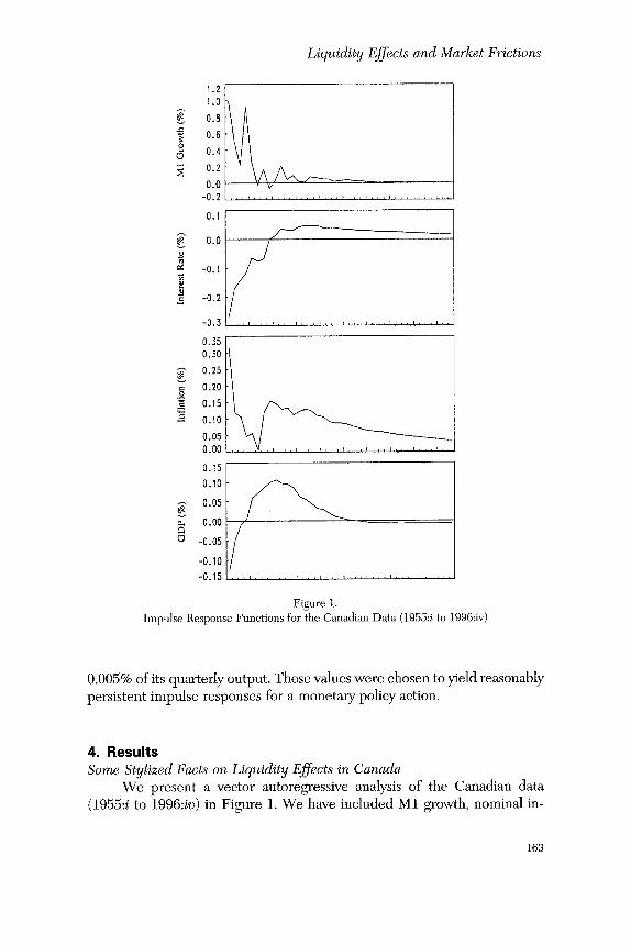
/ Figure 1.
Impulse Response Functions [br the Canadian Data (1955:i to 1996:iv)
0.005% of its quarterly output. These values were chosen to yield reasonably persistent impulse responses for a monetary policy action.
4. Results Some Stylized Facts on Liquidity Effects in Canada
We present a vector autoregressive analysis of the Canadian data (1955:i to 1996:iv) in Figure 1. We have included M1 growth, nominal in-
163
Scott Hendry and Guang-Jia Zhang
terest rate, inflation and output in the VAR in tile order as shown in the Figure. In addition, we impose a Choleski decomposition on VAt/ to help identify the assumptions, s Doing so implies that the poliey action is purely exogenous to the economic system in our VAIl analysis. Following a one- standard deviation shock to MI growth, the short-term nominal interest rate falls immediately by about 30 basis points. In the subsequent quarters, this liquidity effect beeomes dominated by the expected inflation effect and the interest rate starts to increase gradually. After about six quarters, the interest rate moves above steady state. The various poliey shock identification tech- niques usually estimate liquidity effects that last between three and six quar- ters for Canada.
The low interest rate leads to an extended expansion of output lasting for three to four years, The policy shock has an immediate impaet on inflation in tile first quarter. The inflation responds immediately then falls back to- ward steady state before jumping up again to another peak about six to eight quarters following the shock. The peak impact on inflation is only about 30 basis points but the deviation of inflation from control persists for much longer than output.
hnpacts of an Expansionary Policy Shock: Impulse Ilesponses This section analyzes the model through a discussion of the model's
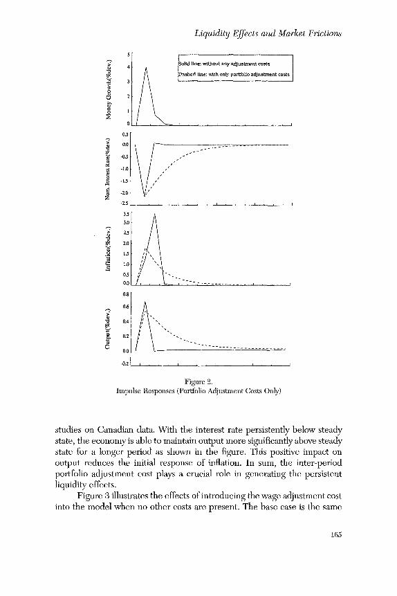
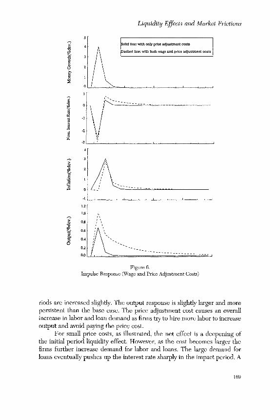
impulse responses to a one-period moneta~ 7 poliey action. The innovation, a~t, in Equation (91) is set to 0.01, representing a 4% annualized money growth rate shoek. The impulse response functions for the interest rate, inflation rate, and output are plotted in each of Figures 2 to 6 for different adjustment cost assumptions. Figures 9., 3, and 4 show the impulse responses when portfolio, wage, and price adjustment costs, respectively, are added to the basic limited-participation model. Figure 5 shows the model responses when all of the costs are eombined. To illustrate that the model can respond differently depending on the combination of costs assumed, Figure 6 shows the effects of adding wage costs when there are also price costs present.
The base case in Figure 2 is a model with the limited-participation assumption. As expected, this model generates too much liquidity effect compared with the Canadian data. In addition, the effects of a policy action on all variables are short-lived.
However, the presenee of tile inter-period portfolio adjustment cost slows down the flows of funds between households (savers) and banks (initial borrowers), Consequently, banks are flush with cash longer so the liquidity effect becomes much more persistent, which is eonsistent with empirical
6The readers can find the more detailed VAIl analysis of the Canadian data in Fung and Kasumovieh (1998) which yields similar results to those shown here.
164
g
O.S
0.0
-0.5
-I.0 .o o -1.5 _=
-z.0
-2.5
3.5 3.0
~ z5
~ 2.0
.~ 1.5 N
1.0
0.5 0.0
0.8
0.6
"~ 0.4-
~ 0.2
0.0
-0.2
Liquidity Effects and Market Frictions
~ oltd line: without any adjustment costs i I ~ ~ashed llne: with only portfolio adjustment costs
studies on Canadian data. With the interest rate persistently below steady state, the economy is able to maintain output more significantly above steady state for a longer period as shown in the figure. This positive impact on output reduces the initial response of inflation. In sum, the inter-period portfolio adjustment cost plays a crucial role in generating the persistent liquidity effects.
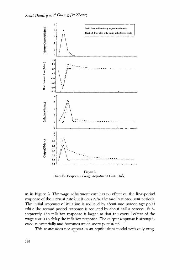
Figure 3 illustrates the effects of introducing the wage adjustment cost into the model when no other costs are present. The base case is the same
as in Figure 2. The wage adjustment cost has no effect on the first-period response of the interest rate but it does raise the rate in subsequent periods. The initial response of inflation is redueed by about one percentage point while the second period response is reduced by about half a pereent. Sub- sequently, the inflation response is larger so that the overall effect of the wage cost is to delay the inflation response. The output response is strength- ened substantially and beeomes much more persistent.
This result does not appear in an equilibrium model with only exog-
enous price rigidities, such as the model by Chari, Kehoe, and McGrattan (1996). In their model, a certain fraction of firms cannot change their prices in a short period of time. However, these firms can always adjust their pro- duction to meet the market demand in equilibrium. That is, the market supply can always meet the market demand spurred by the shock. In con- trast, in our model an expansionary policy shock increases equilibrium em- ployment and wages. The wage adjustment cost prolongs the wage adjust- ment process, thereby causing households to increase their labor supply
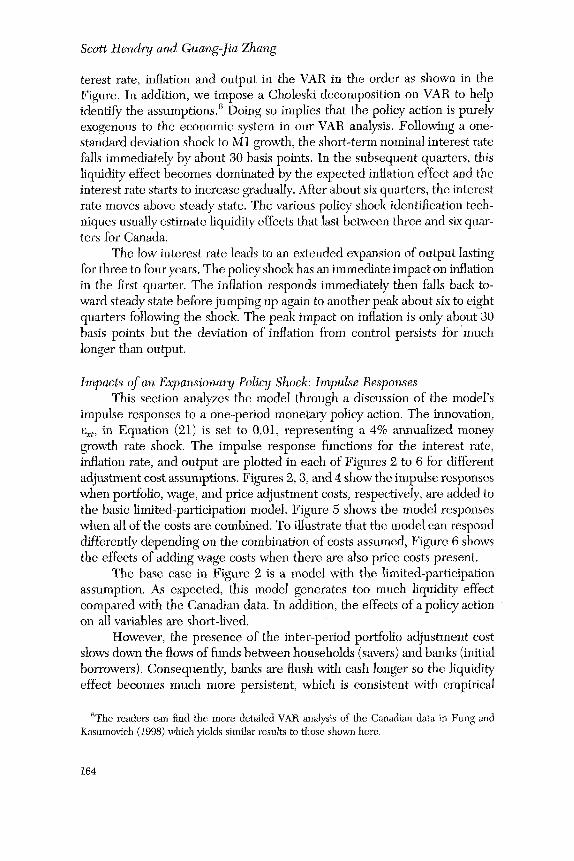
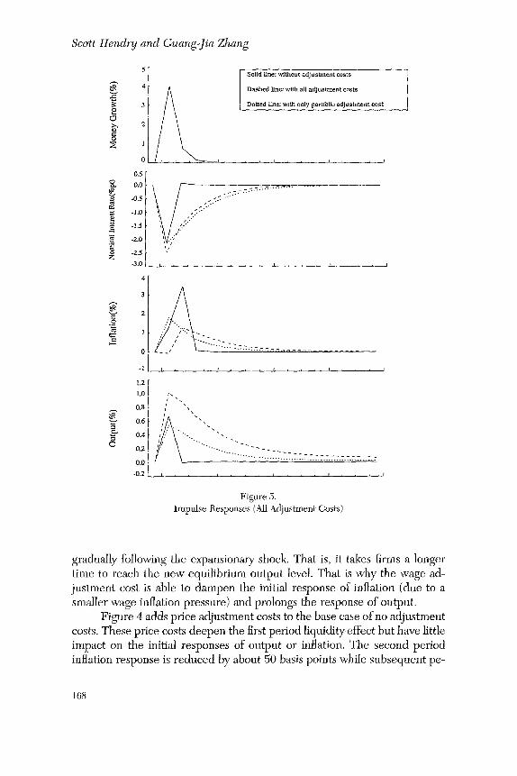
I m p u l s e R e s p o n s e s (All A d j u s t m e n t C o s t s )
gradually fbllowing the expansionary shock. That is, it takes firms a longer time to reach the new equilibrium output level. That is why the wage ad- justment cost is able to dampen tile initial response of inflation (due to a smaller wage inflation pressure) and prolongs the response of output.
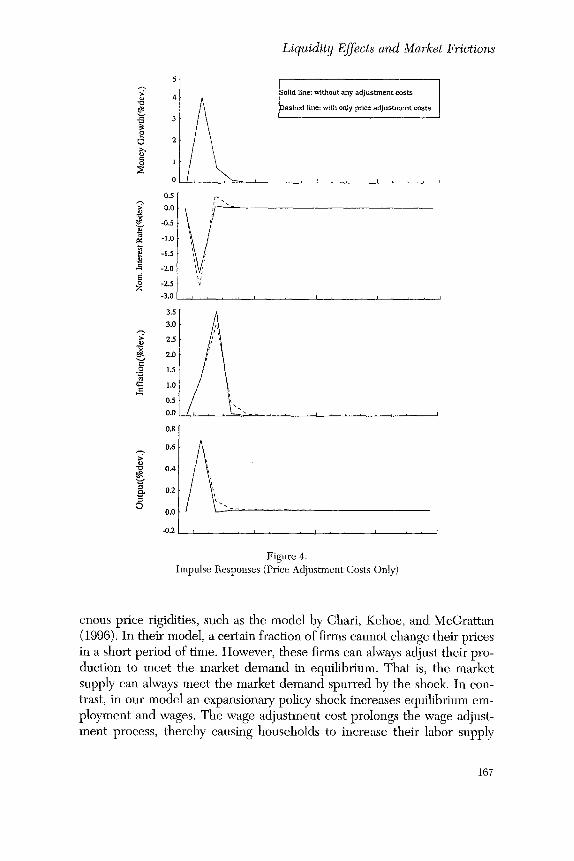
Figure 4 adds priee adjustment costs to the base case of no adjustment costs. These price costs deepen the first period liquidityeffect but have little impact on the initial responses of output or inflation. Tile second period inflation response is reduced by about 50 basis points while subsequent pe-
J 6 8
5
4
.¢: 3
p 2
0
1
e~
_=
Z -3
4
,~. 3
*¢j
g
o
-1
1.2 1.0 0.8
~, 0.6 ~¢~ 0.4
02 011
Liquidity Effects and Market Frictions
~ llne: w i t h l l d line: with only pflce adjustment costs [ i
both wage and price adjustment c o s t s
I * , , , r i , I L I
I I I
i s ~
I , , - T - - - r
Figure 6. Impulse Response (Wage and Price Adjustment Costs)
riods are increased slightly. The output response is slightly larger and more persistent than the base case. The price adjustment cost causes an overall increase in labor and loan demand as firms try to hire more labor to increase output and avoid paying the price cost.
For small price costs, as illustrated, the net effect is a deepening of the initial period liquidity effect. However, as the cost becomes larger the firms further increase demand for labor and loans. The large demand for loans eventually pushes up the interest rate sharply in the impact period. A
169
Scott Hendry and Guang-Jia Zhang
sensitivity analysis reveals that the interest rate becomes unrealistically vol- atile long before the inflation response is dampened in any substantial manner.
Figure 5 shows the combined effect of all three adjustment costs on the model. The liquidity effect is deepened such that the interest rate is at least one percentage point below steady state for several quarters. The in- flation response is reduced substantially over the first two periods and sub- sequently becomes much more persistent. The output response is much larger and more persistent than in the base case. Note that the persistent liquidity effect is the result of the portfolio adjustment cost while the wage and price costs reduce and delay the inflation response. All three costs add persistence to the output response, but it is the wage cost which increases its magnitude the most.
To illustrate that there can be important interactions between the ad- justment costs. Figure 6 shows the effects of adding a wage cost to a model that already has a price adjustment cost. In comparison to the results shown in Figure 3, where the wage cost had no effect on the first period interest rate, we see that the wage cost now deepens the initial liquidity effect. This will only occur if there is a price cost present. The larger is the price cost, the more effective is the wage cost at deepening the initial period liquidity effect.
Higher Moments' This section analyzes the higher moments of a number of different
versions of the model to illustrate some of the relative contributions of each of the adjustment costs.
Table 1 contains some summary statistics for Canada from 1955 to 1996 for the primary real and nominal variables. The stylized facts are: (1) interest rate is quite smooth; (2) price is as volatile as output; (3) inflation is more variable than output.
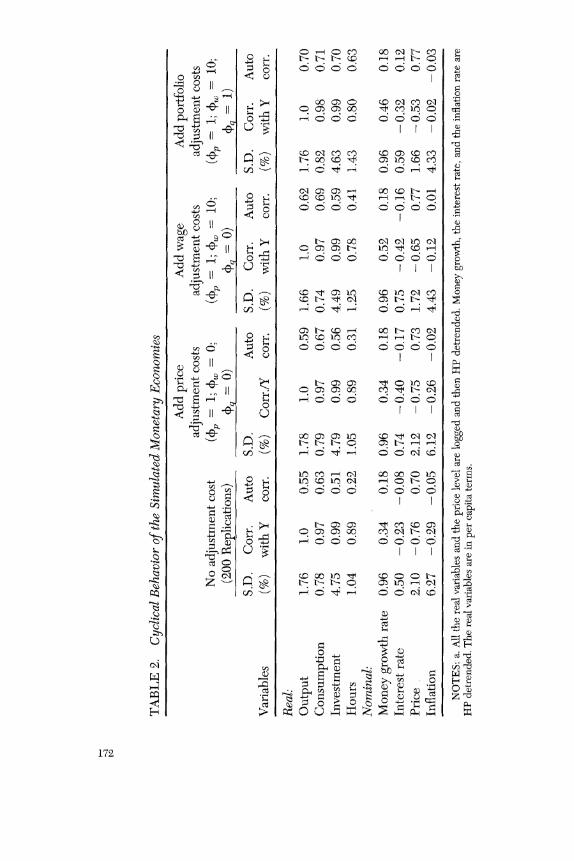
A 42-year sample was replicated 200 times assuming G 0 = 0.01 and ¢r x = 0.0096. Tile model's trend was reintroduced into the simulated data before it was logged and HP detrended. The summary statistics for certain variables of interest are given in Table 2. The first set of columns in Table 2 shows the results of the model when there are no adjustment costs. The next three sets of columns add price adjustment costs, followed by wage adjustment costs, and, finally portfolio adjustment costs.
On the real side, comparing Tables 1 and 2 shows that the standard deviations of output and consumption are quite close to that found in the Canadian data although the simulated investment series are not as volatile as they should be. In general, our model, like other dynamic general equi-
170
TABLE 1. 1996:iv
Liquidity Effects and Market Frictions
Cyclical Behavior of the Canadian Economy: 1955:i to
Standard Correlation Variables Deviation (%) with real GDP Autocorrelation
NOTES: a. All the real variables and the price level are logged and then HP detrended. Money growth, the interest rate and the inflation rate are HP detrended. The real variables are in per capita terms. The data on hours worked spans the 1976 to 1996 period only. We also apply this same procedure to the time series generated from the model.
librium models, can mimic reasonably well the cyclical behavior of the real economy.
On the nominal side, all nominal variables are more volatile than in the actual data. All three adjustment costs reduce the volatility of inflation but not by enough to replicate the variance observed in the Canadian data. The price adjustment costs greatly increase the volatility of the nominal interest rate. This implies that the real interest rate also becomes more volatile given that price adjustment costs reduce the inflation volatility. That is why the real variables also fluctuate more with the addition of price ad- justment costs. The portfolio adjustment costs offset some of the volatility of the interest rate, but not enough to allow the price adjustment costs to be increased until the model's inflation volatility matched the Canadian data.
All versions of the model exhibit negative correlations of the interest rate, price level, and inflation rate with output while the actual data has a negative correlation between only output and the price level. The negative interest rate-output correlation is the result of the central bank following a money growth rate rule instead of a more counter cyclical rule, as has been true over history. The negative inflation-output correlation, while reduced by the adjustment costs, is probably due to an excessive reliance on tech- nology shocks instead of demand shocks to obtain the proper output vari- ance. As well, the wage adjustment costs are most useful for trying to reverse
the negative correlations of the inflation rate with output. The basic version of the model also has a negatively autoeorrelated interest rate, contrary to the Canadian data, which only the portfolio adjustment cost is capable of reversing. Our findings imply that the market adjustment costs can help generate the persistence in output fluctuations, but still cannot successfully replicate the variation of the nominal side of the Canadian economy.
5. Concluding Remarks This paper examines how different types of market frictions can affect
the transmission of monetary policy. It is shown that different types of real and nominal side adjustment costs earl be used to improve the impulse re- sponse functions and higher moment characteristics of limited-participation models.
The price adjustment cost could not effectively reduce inflation vola- tility without first introducing excessive interest rate volatility. In contrast, wage and portfolio adjustment costs are relatively more effective than the price rigidity at reducing the nominal volatility in the economy. For modest levels of price adjustment costs, this relative inability to lower inflation occurs because the changes in the firm's behavior caused by the price cost create subsequent effects that offset the firm's desire to minimize the price cost. For instance, higher price adjustment costs increase labor demand, which pushes up wages and hence consumer demand and prices. These offsetting effects limit the price cost's ability to reduce inflation volatility in this model.
The model also reveals some important interactions between the ad- justment costs. Price adjustment costs were even less effective at reducing inflation volatility when there were portfolio costs present in the model. Also, in contrast to results found in the sticky wage literature, the wage adjustment costs could deepen the liquidity effect in this model but only if there were price adjustment costs already present.
Received: August 1999 Final version: April 2000
References Aiyagari, S. Rao. "Macroeconomics with Frictions." Federal Reserve Bank
of Minneapolis Quarter Review (Summer 1997): 28-41. Aiyagari, S. Rao, and R. Anton Braun. "Some Models to Guide the Fed."
Carnegie-Rochester Public Policy Conference Series 48(0) (June 1998): 1-42.
Andolfatto, David, and Paul Gomme. "Monetary Policy Regimes and Be-
173
Scott Hendry and Guang-Jia Zhang
liefs." Federal Reserve Bank of Cleveland, Working Paper No. 9905, July 1999.
Armstrong, John, Richard Black, Douglas Laxton, and David Rose. "The Balk of Canada's New Quarterly Projection Model, Part 2: A Robust Method for Simulating Forward-Looking Models." Bank of Canada, Technical Report No, 73, February 1995.
Basu, Susanto. "Intermediate Goods and Business Cycles: Implications of Productivity and Welfare.'" American Economic Review 85 (June 1995): 512-30.
Beaudry, Paul, and Michael Devereux. "Towards an Endogenous Propaga- tion Theory of Business Cycles." Manuscript, University of British Co- lumbia, 1996.
Carlstrom, Charles, and Tim Fuerst. "The Benefits of interest Rate Target- ing: A Partial and a General Equilibrium Analysis." Federal Reserve Bank of Cleveland Economic Review (Quarter 2 1996): 2-14.
Chari, V. V., Larry Christiano, and Martin Eiehenbaum. "Inside Money, Outside Money and Short-Term Interest Rates." NBER Working Paper #5269, September 1995.
Chaff, V. V., Patrick J. Kehoe, and Ellen R. MeGrattan. "'Sticky Price Models of the Business Cycle: Can the Contract Multiplier Solve the Persistence Problem?" Federal Reserve Bank of Minneapolis Staff Report 217 De- cember 1996.
Cho, J-O, T. Cooley, and L. Phaneuf. "Tile Welfare Cost of Nominal Wage Contracting." Review of Economic Studies 64 (1997): 465-84.
Christiano, Larry. "Modelling the Liquidity Effect of a Money Shock." Fed- eral Reserve Bank of Minneapolis Quarterly Review (Winter 1991): 3-34.
Christiano, Larry, and Martin Eichenbaum. "Identification and the Liquidity Effect of a Monetary Policy Shock." In Business Cycles, Growth and Political Economy, edited by L. Hercowitz and L. Leiderman, Can> bridge, Mass.: MIT Press, 1992.
- - . "Liquidity Effects, Monetary Policy, and tile Business Cycle." Fed- eral Reserve Bank of Minneapolis, Institute for Empirical Macroeconom- ics, Discussion Paper 70, 1992a.
- - . "Liquidity Effects and the Monetary Transmission Mechanism." American Economic Review 82, no. 2 (May 1992b): 346-53.
Christiano, Larry, Martin Eichenbaum and Charles Evans. "The Effects of Monetary Policy Shocks: Evidence from the Flow of Funds." The Review of Economics and Statistics 78, no. 1 (February 1996): 16-34.
- - . "Modeling Money." NBER Working Paper #6371, January 1998, Coleman II, W. John. "Equilibrium in a Production Economy with an In-
come Tax." Econometrica 59, no. 4 (July 1991): 1091-1104.
174
Liquidity Effects and Market Frictions
Cooley, Tom F., and Gary D. Hansen. "The Inflation Tax in a Real Business Cycle Model." American Economic Review 79, no. 4 (September 1989): 733-48.
- - . "Tile Welfare Costs of Moderate Inflations." Jourr~al of Money, Credit, and Banking 23, no. 3 (August 1991): 183-503.
Dow, James P., Jr. "The Demand and Liquidity Effects of Monetary Shocks." Journal of Monetary Economics 36, no. 1 (August 1995): 91-115.
Finn, Mary. "The Increasing-Returns-to-Seale/Sticky-Price Approach to Monetary Analysis." Federal Reserve Bank of Richmond Economic Quar- terly 81, no. 4 (1995): 79-93.
Fuerst, Tim. "Liquidity, Loanable Funds, and Real Activity."Journal of Mon- etary Economics 29 (1992): 3-24.
Fung, Ben, and Marcel Kasumovich. "Monetary Shocks in the G-6 Coun- tries: Is There a Puzzle?" Journal of Monetary Economics 42, no. 3 (De- cember 1998): 575-92.
Gomme, Paul, and Jeremy Greenwood. "On the Cyclical Allocation of Risk." Journal of Economic Dynamics and Control 19, nos. 1, 2 (January 1995): 91-124
Goodfriend, Marvin, and Robert King. "The New Neoclassical Synthesis and the Role of Monetary Policy." NBER Macroeconomics Annual (1997): 231-95.
Hamilton, James. Time Series Analysis. New Jersey: Princeton University Press. 1994.
Hendry, Scott, and Guang-Jia Zhang. "Liquidity Effects and Market Fric- tions." De Nederlandsehe Bank, Staff Reports No. 29, 1999.
Kim, Jinill. "Monetary Policy in a Stochastic Equilibrium Model with Real and Nominal Rigidities." Manuscript, Yale University, 1996.
Kimball, Miles. "The Quantitative Analytics of the Basic Neomonetarist Model." Journal of Money, Credit, and Banking 27(4) (November 1995): 1241-77.
Lncas, Robert E., Jr. "'Liquidity and Interest Rates." Journal of Economic Theory 50, no. 2 (April 1990): 237-64.
Rotemberg, Julio. "Prices, Output and Hours: an Empirical Analysis Based on a Sticky Price Model." Journal of Monetary Economics 37, no. 3 (June 1996): 505-33.
Taylor, John. "Aggregate Dynamics and Staggered Contracts." Journal of Political Economy 88, no. i (February 1980): 1-23.
• "Temporary Price and Wage Rigidities in Macroeconomics: A Twenty-Five Year Review." Manuscript, Stanford University. 1997.
Williamson, Steve. "Real Business Cycle Research Comes of Age: A Review Essay." Journal of Monetary Economics 38, no. 1 (August 1996): 161-70.
175
Scott Hendry and Guang-Jia Zhang
Appendix: Model Details Model Solution Technique
The model is solved using a technique which "stacks" the first-order conditions and market clearing conditions, one for each endogenous variable at each period of a proposed horizon, and then solves the complete system simultaneously using a Newton procedure. A more complete description of this "stacked time" methodology and a comparison to similar techniques can be found in Armstrong et al. (1995). Two of the primary benefits of this technique are that it does not involve a linear approximation so that the model's important nonlinearities are not lost, and that it converges on a solution relatively easily and quickly.
The derivation of the stationary representation of tile equilibrium is available upon request. It is also given in Hendry and Zhang (1999).