Working Paper/Document de travail2007-39

Liquidity, Redistribution, and theWelfare Cost of Inflation

by Jonathan Chiu and Miguel Molico

www.bankofcanada.ca

Bank of Canada Working Paper 2007-39

July 2007

Liquidity, Redistribution, and theWelfare Cost of Inflation

by

Jonathan Chiu and Miguel Molico

Monetary and Financial Analysis DepartmentBank of Canada

Ottawa, Ontario, Canada K1A 0G9jchiu@bankofcanada.ca

mmolico@bankofcanada.ca

Bank of Canada working papers are theoretical or empirical works-in-progress on subjects ineconomics and finance. The views expressed in this paper are those of the authors.

No responsibility for them should be attributed to the Bank of Canada.

ISSN 1701-9397 © 2007 Bank of Canada

ii

Acknowledgements

We have benefited from the comments and suggestions of participants at the CEA meetings in

Montreal, the Money, Banking and Payments Workshops at the Cleveland Fed, Midwest

Macroeconomics conference in St. Louis, the SED conference in Vancouver, and the Dynamic

Models Useful for Policy Making conference at the Bank of Canada. Special thanks are due to

Jeannie Kottaras for her assistance with Canadian monetary aggregates’ data and to Steve Ambler,

Walter Engert, Cesaire Meh, and Randall Wright for their comments on an earlier draft of this

paper.

iii

Abstract

This paper studies the long run welfare costs of inflation in a micro-founded model with trading

frictions and costly liquidity management. Agents face uninsurable idiosyncratic uncertainty

regarding trading opportunities in a decentralized goods market and must pay a fixed cost to re-

balance their liquidity holdings in a centralized liquidity market. By endogenizing the

participation decision in the liquidity market, this model endogenizes the responses of velocity,

output, the degree of market segmentation, as well as the distribution of money. We find that,

compared to the traditional estimates based on a representative agent model, the welfare costs of

inflation are significantly smaller due to distributional effects of inflation. The welfare cost of

increasing inflation from 0% to 10% is 0.62% of income for the U.S. economy and 0.20% of

income for the Canadian economy. Furthermore, the welfare cost is generally non-linear in the

rate of inflation, depending on the endogenous responses of the liquidity market participation to

inflation and liquidity management costs.

JEL classification: E40, E50Bank classification: Inflation: costs and benefits

Résumé

Les auteurs étudient les coûts à long terme de l’inflation au plan du bien-être dans un modèle avec

fondements microéconomiques où les échanges s’accompagnent de frictions et d’une gestion des

liquidités coûteuse. Les agents sont confrontés à une incertitude idiosyncratique inassurable qui

touche les occasions d’échange sur un marché décentralisé des biens, et ils doivent rééquilibrer

leurs avoirs liquides à coût fixe sur un marché centralisé des liquidités. En conférant un caractère

endogène à la décision des agents de participer au marché des liquidités, les auteurs permettent au

modèle d’endogénéiser les réactions obtenues pour la vitesse de circulation, la production, le

degré de segmentation des marchés et la distribution de la monnaie. Ils constatent que, par rapport

aux estimations conventionnelles des modèles à agent représentatif, les coûts de l’inflation sur le

bien-être se trouvent nettement réduits par les effets de répartition de l’inflation. Ainsi, la hausse

du taux d’inflation de 0 à 10 % se solde, en termes de bien-être, par une perte de revenus de

0,62 % pour l’économie américaine et de 0,20 % pour l’économie canadienne. De plus, la perte

de bien-être n’évolue souvent pas dans les mêmes proportions que le taux d’inflation, mais

dépend de l’effet endogène qu’a l’inflation sur la participation au marché des liquidités ainsi que

des frais de gestion des liquidités.

Classification JEL : E40, E50Classification de la Banque : Inflation : coûts et avantages

1 Introduction

The adoption of formal inflation targets by Canada and other countries during the last

decades and the generalized move towards lower inflation by most countries has stimulated a

considerable interest in the welfare gains from price stability. In this paper, we contribute to

this debate by evaluating the long-run welfare costs of inflation in a micro-founded monetary

model with trading frictions, modeled as uninsurable idiosyncratic uncertainty regarding

trading opportunities, and costly liquidity management.

The measurement of the welfare costs of inflation is one of the classic questions in mon-

etary economics and has been addressed in a long line of research starting with the con-

tributions of Bailey (1956) and Friedman (1969). In his seminal paper, Bailey proposed

quantifying the welfare cost of inflation by measuring the “welfare triangle,” the area un-

der the money demand curve representing the consumers’ surplus that could be gained by

reducing the nominal interest rate from r to zero. In a recent paper, Lucas (2000) surveys

research on the welfare cost of inflation and provides new estimates for the U.S. economy.

Lucas estimates the welfare gain of going from 10% to 0% inflation to be slightly below 1

percent of income. The magnitude of the estimate of such costs is not without controversy

and, in particular, depends critically on the interest and transaction sensitivity of the money

demand.1 Given that there are few historical episodes of very low and very high nominal

interest rates for which data is available, the robust estimation of such critical parameters

as the interest elasticity of the money demand becomes particularly challenging. Guidance

from solid micro-founded monetary theory becomes essential to understand how individuals

manage their liquidity. In Lucas’ own words, “[...] theory at the level of the models I re-

viewed [...] is not adequate to let us see how people would manage their cash holdings at very

low interest rates. Perhaps for this purpose theories that take us farther on the search for

foundations, such as the matching models introduced by Kiyotaki and Wright, are needed.”

1Lucas’ estimate is double the estimates of Bailey’s and others. The reason for these higher costs is thatLucas uses a double log schedule for the money demand, as opposed to the semi-log schedule utilized byBailey and Friedman, arguing that it provides a better fit to twentieth-century U.S. data.

2

In this paper we pursue exactly this challenge.

A recent paper by Lagos and Wright (2005) proposes a new framework for monetary and

policy analysis based on a micro-founded search theoretical model of money and provides

new measures of the welfare costs of inflation. They calibrate their model to match the U.S.

empirical money demand curve and find a much higher welfare cost than standard estimates.

Their model predicts that going from 10% to 0% inflation can be worth between 3% and

5% of consumption. The reason for these higher welfare costs are the distortions (hold-

up problems) introduced by the non-competitive pricing mechanism assumed - generalized

Nash-bargaining. In the absence of these distortions, e.g., when buyers get to make take-it-

or-leave-it offers to sellers, their estimates are similar to those of Lucas.2

One limitation of the analysis conducted by Lagos-Wright is that, for the sake of an-

alytical tractability, they make restrictive assumptions that eliminate some of the most

interesting features of standard search models of money, features that could have important

implications for the measurement of the welfare costs of inflation. In particular, in standard

search models uninsurable idiosyncratic uncertainty regarding trading opportunities, and

thus the timing and amounts of receipts and disbursements of money (an empirically plau-

sible feature), leads to a non-trivial liquidity management problem and, in equilibrium, to

a non-degenerate distribution of money across agents. In such an environment, agents hold

money for both transactions and precautionary motives and an expansionary redistributive

monetary policy can potentially be welfare improving by providing “insurance” against an

agent’s idiosyncratic trading history.3 On the other hand, Lagos and Wright allow agents

2In their model agents must make an irreversible decision, while in a centralized market, on how muchmoney to bring into the bargaining table in the decentralized market. The more money an agents bringsthe bigger the surplus of trade to be had at a bilateral meeting. Yet, unless the buyer has all the bargainingpower, he will only get part of that additional surplus. As such, agents will generally bring too little moneyinto the decentralized market. Inflation, by decreasing the amount of real money balances agents want tocarry in equilibrium, further accentuates this distortion leading to the higher welfare costs of inflation.

3For example, see Deviatov and Wallace (2001) and Molico (2006). Similar results are found in Levine(1991), in a distinct environment. In contrast, Imrohoroglu (1992) finds that, in an endowment economywhere agents hold money in order to smooth consumption in the face of income variability for which thereis no insurance, the welfare costs of inflation are significantly higher than previous estimates since inflationhinders the ability of agents to smooth consumption.

3

to costlessly re-balance their money holdings without limit by producing and trading “gen-

eral goods” in a centralized market after each round of decentralized trade. By assuming

agents have quasilinear preferences over such goods they effectively provide a mechanism

through which agents can perfectly “insure” against their idiosyncratic trading histories. By

construction, this assumption eliminates any redistributive gains from inflation making it

impossible to determine if these effects are quantitatively significant. As mentioned above,

these assumptions are made for the sake of analytical tractability and not for their empirical

plausibility.

Our paper relaxes these assumptions by considering an environment in which the par-

ticipation in a centralized liquidity market is both costly and endogenous. In particular, we

assume that agents have to pay a fixed cost to participate in such a market.4 This assump-

tion is meant to capture the idea that participation in organized trading, intermediation and

financial market is costly. These costs include not only financial costs of participation but

also time spent in such activities. Moreover, it is motivated by the fact that not all house-

holds actively and frequently participate in these activities, and that the participation rate

depends on the state of the economy (e.g., inflation and financial development). Because

of this market participation friction, agents choose to attend the centralized market only

infrequently and to keep an inventory of money for trading in the decentralized market. In

this sense, our model provides micro-foundations for a class of inventory theoretic monetary

models in the tradition of Baumol (1952) and Tobin (1956).5 In our model, the centralized

market provides only limited “insurance” against idiosyncratic uncertainty. By endogenizing

the decision of participation, this model also endogenizes the responses of velocity, output,

the degree of market segmentation as well as the monetary distribution. We calibrate the

4We interpret this market as a “pure liquidity market” in the sense that we assume agents have linearpreferences over the goods traded in such market. As such, the only reason an agent would participate inthis market would be to re-balance his or her money holdings, given that market participation is costly andthere is no other gains of trade to be had. This market is meant to proxy for a number of markets in theactual economy in which agents can obtain insurance against liquidity risk, for example, financial markets.

5For general equilibrium versions of inventory theoretic models of money see, for example, Jovanovic(1982) and Romer (1986).

4

model to match both the U.S. and Canadian empirical money demands and use a numerical

algorithm to study the long-run effects of inflation on welfare for both economies.

The costs and benefits of inflation in our model are threefold. First, as is common in

most monetary models, inflation serves as a distortionary tax reducing welfare. Second, infla-

tion generates deadweight loss associated with the liquidity management activities. Finally,

mildly expansionary redistributive monetary policy can potentially be welfare improving by

relaxing the liquidity constraint of some agents. In this way, inflation works as an “insurance”

mechanism against an agents’s liquidity risk.

Our findings confirm that the consideration of costly liquidity management and distribu-

tional effects quantitatively matter for the welfare cost of inflation. First, we find that the

welfare cost differs significantly from that of a representative agent model and is not well

captured by the area under the aggregate money demand. In particular, abstracting from

the hold-up problem mentioned above, the welfare cost is generally lower than the traditional

estimates due to the distributional effects of inflation. Namely, for example, we find that

the welfare gain of reducing inflation from 10% to 0% to be 0.62% of income for the U.S.

economy and 0.20% of income for the Canadian economy. The corresponding areas under

the aggregate money demand curves (which are approximately equal to the welfare cost in

a representative agent model) are, respectively, 0.85% and 0.34%. It is worthwhile noticing

that the welfare costs of a 10% inflation for the Canadian economy is one third of that of

the U.S. economy. This finding is consistent with previous estimates of the welfare costs of

inflation for both economies using a representative agent models and is a reflection of the

lower interest-elasticity of the Canadian money demand implied by the data. Furthermore,

as is the case for the U.S. economy, our estimate is lower than previous estimates in the

literature.6

Second, the welfare cost is generally non-linear in the rate of inflation. The welfare

6For example, Serletis and Yavari (2004) redo the estimates of Lucas for the Canadian economy usingrecent advances in the field of econometrics to estimate the interest elasticity of money demand and reporta welfare cost of 0.35% from reducing the nominal interest rate from 14% to 3%, similar to the area underthe demand curve that we estimate.

5

cost of small rates of inflation might be proportionally smaller or larger than that of higher

rates depending on how the participation rate in the liquidity market and associated costs

responds to inflation. This implies that the welfare costs of 10% inflation might not be too

informative if one is interested in evaluating the welfare gains of reducing inflation, say, from

2% to 1%. Moreover, the effect of a decrease in the costs of participation in the liquidity

market, say due to financial development, on the welfare cost of different rates of inflation

might vary both quantitatively and qualitatively.

This paper is related to other papers in the search-theoretical literature that extend the

Lagos and Wright framework by assuming that agents can trade in the centralized market

only infrequently. Berentsen, Camera and Waller (2005), Ennis (2005), Williamson (2006),

and Telyukova and Wright (2005) study an environment in which agents participate in the

centralized market at an exogenous rate. This paper takes a further step to fully endogenize

the participation in the centralized market because the participation decision should not be

taken as invariant to policy intervention. This paper also generalizes the existing search

literature by developing a framework that nests several existing search models as special

cases. When the fixed cost is zero, the model reduces to Lagos and Wright (2005) in which

the Friedman rule is optimal. When the cost is infinite, the model reduces to Molico (2006)

in which positive inflation can be welfare improving. Finally, this paper also contributes to

the literature by integrating an endogenous market segmentation model (focusing on market

participation frictions)7 with a search-theoretic model (focusing on goods trading frictions).

The rest of the paper is organized as follows. Section 2 describes the environment. Section

3 defines an equilibrium. Section 4 discusses the numerical algorithm used to compute the

stationary equilibria of the model. In section 5, to facilitate the comparison of our results

to the existing literature, we calibrate the model to match the empirical money demand for

the U.S. economy and study the welfare cost of inflation. In section 6 we redo the exercise

7Models with exogenous market segmentation include Grossman and Weiss (1983), Alvarez and Atkeson(1997), and Alvarez, Atkeson and Edmond (2003). Models with endogenous market segmentation includeAlvarez, Atkeson and Kehoe (1999), Chiu (2005) and Khan and Thomas (2005). All these models imposean exogenous cash-in-advance constraint.

6

for the Canadian economy. Section 7 concludes the paper.

2 The Model

Time is discrete and denoted by t = 0, 1, 2, .... There are two types of non-storable com-

modities: general and special goods. The economy consists of a continuum [0, 1] of agents.

The per-period utility of an agent is given by

U(Xt)− C(Yt) + u(xt)− c(yt),

where U(X) denotes the utility of consuming X units of the general good, C(Y ) denotes the

disutility of producing Y units of the general good, u(x) denotes the utility of consuming x

units of the special good, and c(y) denotes the disutility of producing y units of the special

good. We assume that U(X) = X and C(Y ) = Y .8 Also, we assume that u(·) is twice

continuously differentiable, strictly increasing, concave (with u strictly concave), and satisfy

u(0) = 0 with u′(x) = 1 for some x > 0. Also, c(y) = y. Agents discount the future at

discount factor β ∈ (0, 1).

In this economy, there is an additional, perfectly divisible, and costlessly storable object

which cannot be produced or consumed by any private individual, called fiat money. Agents

can hold any non-negative amount of money m ∈ R+. The money stock at the beginning of

period t is denoted Mt. In what follows we express all nominal variables as fractions of the

beginning of the period money supply (before the current period’s money transfers which we

will describe below), m ≡ mM

. Let νt : BR+ → [0, 1] denote the probability measure associated

with the money (as a fraction of the beginning of period money supply) distribution at the

8The assumption of linear utility will allow us to interpret the general goods market as a “pure liquiditymarket” in the sense that there is no surplus of trade to be had in such market. As will be shown, theonly reason agents participate in that market is to re-balance their money holdings. Under appropriateassumptions to preclude their circulation in the decentralized market, one could introduce nominal bondsin this market and interpret the trades as financial asset trades. In that world, in equilibrium, agentsare indifferent between using bonds or trading the general good. In Lagos and Wright, U(X) − C(Y ) isquasi-linear.

7

DAY NIGHT

Money injection

Agents tradespecial goods

Decentralized Market

Centralized Markett t+1

MoneyInjection

Agents makeparticipation

decision

Agents tradegeneral goods

Figure 1: Time line

beginning of period t, where BR+ denotes the Borel subsets of R+.

Each period is divided into two subperiods: day and night. In the day time, there is

a decentralized market for trading special goods. In the night time, there is a centralized

market for trading general goods (see Figure 1).

As in standard search-theoretical models of money, in the decentralized market, agents

are subject to trading frictions modeled as pairwise random matching. To generate the need

for trade, we assume that agents cannot consume their own production of special goods. To

generate the use of money, we assume that the probability of having a double coincidence of

wants meeting is zero and that all trading histories are private information.9 The probability

that an agent consumes something his/her match partner produces is σ ∈ [0, 12]. Similarly,

the probability that an agent produces something that his/her match partner consumes is

σ. Therefore, with a probability 1 − 2σ, trading partners do not want each other’s goods.

9For money to be valued it is only required that in some meetings there is no double coincident of wants.For simplicity, we focus on purely monetary trades and, by assumption, preclude the possibility of barter inthe decentralized market.

8

When two individuals meet and one consumes the good the other produces, they bargain

over the amount of output and the amount of money to be traded. Let qt(mb,ms; νt) ≥ 0

be the amount of output and dt(mb,ms; νt) ≥ 0 the amount of money determined by the

bargaining process at date t between a buyer with money holdings mb and a seller with

ms, when the probability measure at the beginning of the period is νt. In particular, the

terms-of-trade are assumed to be determined by take-it-or-leave-it offers by the buyers.10

Let ωt : BR+ → [0, 1] denote the probability measure over money holdings at the entrance

of the centralized market (after trade in the decentralized market).

At night after the decentralized market closes, there is a Walrasian market for the general

good that opens. Participation in that market is costly. It is assumed that, at the beginning

of each night, each agent i draws a random fixed cost κit (in units of the general good).

The cost κ is assumed to be i.i.d. across time and agents with uniform distribution over

the support [0, κ]. Given the individual’s realization of the fixed cost, an agent must decide

whether or not to participate in the market. Agents take the price of money in terms of

the general good in that market, φt, as given. If an agent chooses not to participate in the

centralized market, he/she consumes zero amount of the general good in autarky. If the

agent decides to participate he/she must decide how much of the general good to consume

and produce, and how much money holdings to carry into the decentralized market the next

day.

Given the environment, the only feasible trades during the day are the exchange of special

goods for money and at night barter in general goods or the exchange of general goods for

money.

The money stock is assumed to grow at a constant growth rate µ = Mt

Mt−1for all t. Money

growth is accomplished via money transfers at the entrance of the decentralized market.

Given the distribution νt, an agent with money holdings m receives a monetary transfer at

10More generally, we could consider that the terms of trade were determined by the solution of a generalizedNash-bargaining problem as in Lagos-Wright. As shown in that paper if the seller has some bargaining poweradditional distortions exist that would imply higher welfare costs of inflation. The same would be true here.In that sense, we provide a lower bound for the welfare costs of inflation.

9

the beginning of the period t decentralized market, τ(m, νt) (as in Lagos-Wright or Molico).11

We assume that the monetary transfers (monetary policy rule) are such that rate of monetary

growth is constant over time.

µ ≡∫ ∞

0

[m + τ(m, νt)] νt(m)dm. (1)

This concludes the description of the environment. In what follows, we will gradually

build towards the definition of equilibrium.

3 Equilibrium

In this section we define a recursive equilibrium for this economy. We begin by describing the

individual and aggregate state variables. An individual’s state variable consists of his/her

money holdings (as a fraction of the beginning of the period money supply). The aggregate

state variable is, in turn, defined as the current probability measure over money holdings.

Thus, at the beginning of the period an individual’s state is described by the pair (m, ν),

and at the entrance of the centralized market by (m,ω). Agents take as given the law of

motion of the aggregate state variable defined by ν ′ = Hν(ω) and ω = Hω(ν) which we will

describe in detail below, where prime denotes the future period.12 Also, agents take as given

the price of money in units of the general good in the centralized market, φ, as a function

of the current aggregate state, φ : Λ → R+ \ {0}, where Λ denotes the space of probability

measures over BR+ .13 Finally, agents take as given the monetary policy rule (transfers)

τ : R+ × Λ → R.

11In principle, money could also be injected by transfers to participants in the centralized market. Thiswould generate an additional “limited participation” effect by redistributing wealth from non-participantsto participants. We study this case in a separate note.

12Equivalently, define the law of motion of by ν′ = H(ν) ≡ Hν(Hω(ν)).13Note that by restricting φ to be strictly positive, we focus on only monetary equilibrium in which money

has value.

10

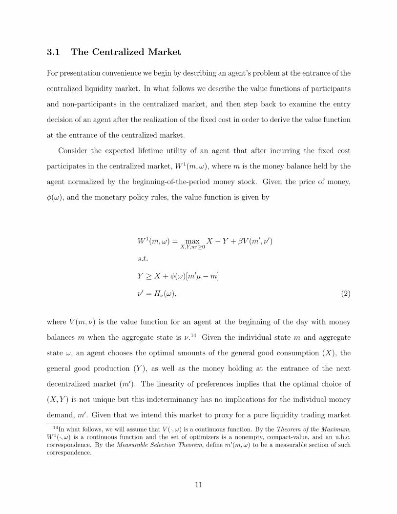
3.1 The Centralized Market

For presentation convenience we begin by describing an agent’s problem at the entrance of the

centralized liquidity market. In what follows we describe the value functions of participants

and non-participants in the centralized market, and then step back to examine the entry

decision of an agent after the realization of the fixed cost in order to derive the value function

at the entrance of the centralized market.

Consider the expected lifetime utility of an agent that after incurring the fixed cost

participates in the centralized market, W 1(m,ω), where m is the money balance held by the

agent normalized by the beginning-of-the-period money stock. Given the price of money,

φ(ω), and the monetary policy rules, the value function is given by

W 1(m,ω) = maxX,Y,m′≥0

X − Y + βV (m′, ν ′)

s.t.

Y ≥ X + φ(ω)[m′µ−m]

ν ′ = Hν(ω), (2)

where V (m, ν) is the value function for an agent at the beginning of the day with money

balances m when the aggregate state is ν.14 Given the individual state m and aggregate

state ω, an agent chooses the optimal amounts of the general good consumption (X), the

general good production (Y ), as well as the money holding at the entrance of the next

decentralized market (m′). The linearity of preferences implies that the optimal choice of

(X,Y ) is not unique but this indeterminancy has no implications for the individual money

demand, m′. Given that we intend this market to proxy for a pure liquidity trading market

14In what follows, we will assume that V (·, ω) is a continuous function. By the Theorem of the Maximum,W 1(·, ω) is a continuous function and the set of optimizers is a nonempty, compact-value, and an u.h.c.correspondence. By the Measurable Selection Theorem, define m′(m,ω) to be a measurable section of suchcorrespondence.

11

(with no value added), we ignore the production and consumption of the general goods in our

measure of aggregate output.15 The budget constraint simply states that the expenditure

on consumption and on net money purchase is no greater than the income from production.

We can show that (see Lagos and Wright for details),

W 1(m,ω) = φ(ω)m + maxm′

[−φ(ω)m′µ + βV (m′, ν ′)].

The expected lifetime utility of an agent not participating in the centralized market with

money holding m is given by

W 0(m,ω) = βV

(m

µ,Hν(ω)

). (3)

Non-participants consume and produce nothing and their money balance (as a fraction

of the beginning of the period money supply) declines at the rate of money growth.

We now consider the decision of whether or not to participate in the centralized market.

Consider the case of an agent at the entrance of the centralized market with money holdings

m when the aggregate state is ω and who draws a fixed cost κ. The agent will participate

in the centralized market as long as

W 1(m,ω)− κ > W 0(m,ω).

Define κ(m,ω) to be the threshold value such that any agent with state (m,ω) that draws

a cost κ chooses to participate if κ < κ(m,ω). The threshold function κ : R+ × Λ → [0, κ]

is defined as

κ(m,ω) = min{max{0,W 1(m,ω)−W 0(m,ω)}, κ}. (4)

Given this threshold function we can define the value function for an agent at the entrance

15We also considered the alternative assumption of measuring as part of GDP the minimum amount ofproduction and trade required for agents to be able to adjust their money holdings to the optimal amount.This did not change any of our results qualitatively and only affected minimally our quantitative results.

12

of the centralized market (before drawing the fixed cost) as

W (m,ω) =

∫ κ(m,ω)

0

[W 1(m,ω)− κ

] 1

κdκ +

∫ κ

κ(m,ω)

W 0(m,ω)1

κdκ,

or simplifying,

W (m,ω) =

[W 1(m,ω)− κ(m, ω)

2

]κ(m,ω)

κ+ W 0(m,ω)

[1− κ(m,ω)

κ

]. (5)

The fraction of agents participating in the centralized market is given by

f(ω) =

∫ ∞

0

κ(m,ω)

κω(dm).

Also, in equilibrium, choices of money holdings, m′(m,ω), satisfy the money market

clearing condition, ∫ ∞

0

κ(m,ω)

κ[m′(m,ω)−m] ω(dm) = 0. (6)

Consider a simple example in which V is concave to illustrate how the centralized market

works. Concavity of V implies that W0 is a concave function as shown in Figure 2(a). In this

example, agents with low money holdings will always choose to pay the fixed cost to sell the

general good for liquidity in the centralized market. Also, agents with high money holdings

will always choose to pay the fixed cost to purchase the general good in the centralized

market. The threshold function is given by the κ(m) curve in Figure 2(b).

3.2 The Decentralized Market

We now consider the bargaining problem of an agent in the decentralized market. Consider

a single coincidence meeting when a buyer holds a money balance mb and a seller holds a

balance ms, after the decentralized market’s money injection, when the aggregate state is

ν. We assume that the buyer makes a take-it-or-leave-it offer to the seller. That is, he/she

13

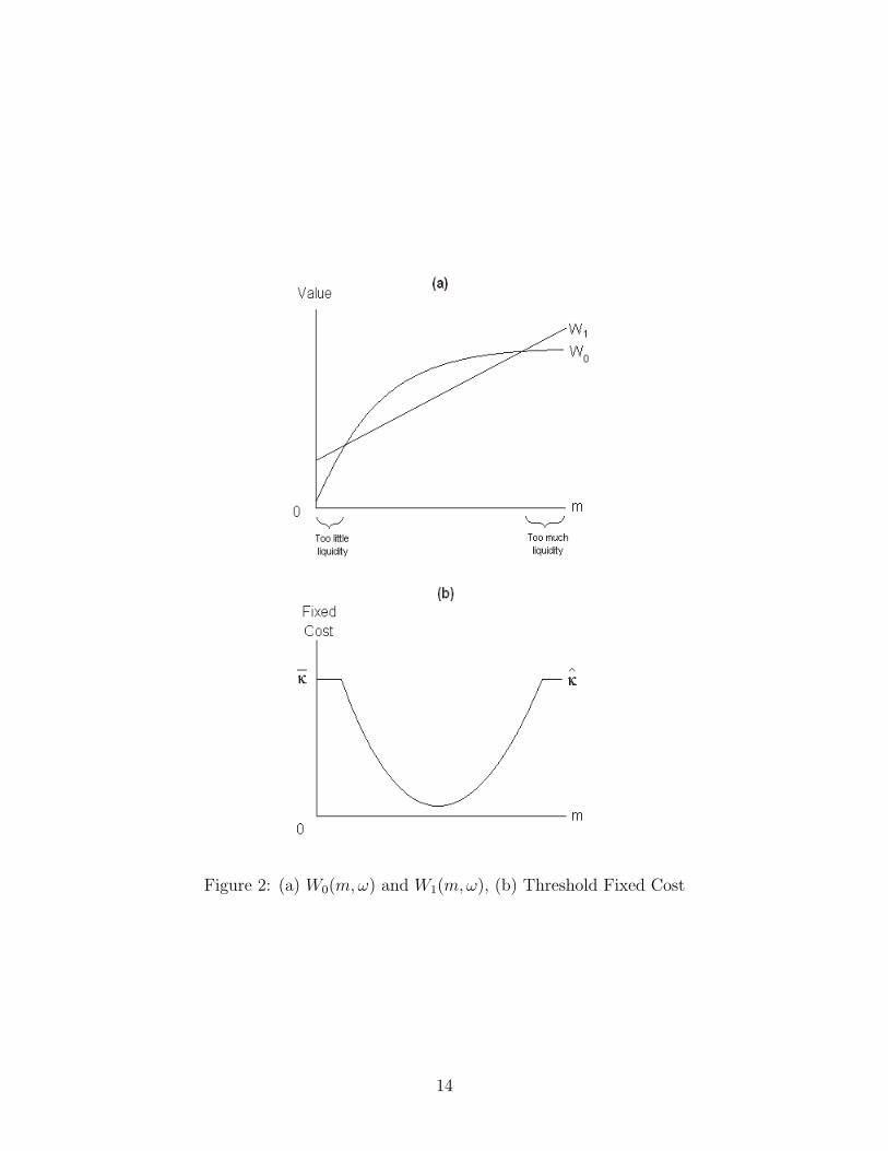
Figure 2: (a) W0(m,ω) and W1(m,ω), (b) Threshold Fixed Cost

14

proposes a trade of an amount of money, d, for a quantity of special good, q, that solve the

following problem:

maxq≥0, 0≤d≤mb

u(q) + W (mb − d,Hω(ν)) (7)

subject to

−q + W (ms + d,Hω(ν)) = W (ms, Hω(ν)).

Or, equivalently, by substituting the latter constraint into the objective function,

max0≤d≤mb

u[W (ms + d,Hω(ν))−W (ms, Hω(ν))] + W (mb − d,Hω(ν)).

The buyer makes an offer to maximize his/her surplus subject to making the seller indifferent

between trading and not trading. Note that, given that W (·, Hω(ν)) is a continuous func-

tion, the objective function of the bargaining problem is continuous. Also, the set d ∈ [0,mb]

is non-empty and compact. Thus, by the Theorem of the Maximum and the Measurable

Selection Theorem, the set of optimizers is a non-empty, compact-valued, and u.h.c. corre-

spondence and admits a measurable selection. Define d(mb,ms, ν) to be such a selection.

The function q(mb,ms, ν) can then be obtained from the seller’s participation constraint.

The expected lifetime utility of an agent that enters the period with money balance m

(before the decentralized market money injection) is given by

V (m, ν) = (1− σ)W [m + τ(m, ν), Hω(ν)] + σ

∫ ∞

0

{u[q(m + τ(m, ν),ms, ν)]

+ W {m + τ(m, ν)− d[m + τ(m, ν),ms, ν], Hω(ν)}} ν(dms). (8)

The first term is the value for an agent that either is a seller, with probability σ, and thus

has a zero net surplus from trade, or meets no one, with probability 1 − 2σ. The second

term is the expected value of being a buyer.

15

3.3 Laws of Motions

Before defining a recursive equilibrium for this economy, we describe the laws of motion

ν ′ = Hν(ω) and ω = Hω(ν). We begin by describing the evolution of the aggregate state

from the beginning of the centralized market to the beginning of the next decentralized

market, Hν . Define the function Π : R+ ×BR+ → [0, 1] to be

Π(m,B; ω) =

1− κ(m,ω)κ

, if mµ∈ B and m′(m, ω) /∈ B;

κ(m,ω)κ

, if mµ

/∈ B and m′(m, ω) ∈ B;

1, if mµ∈ B and m′(m, ω) ∈ B;

0, otherwise.

(9)

Given that, for each m, Π(m, ·; ω) is a probability measure on (R+,BR+), and, for each

B ∈ BR+ , Π(·, B; ω) is a BR+-measurable function, Π is a well defined transition function.

Then, the law of motion Hν(·) can be defined as

ν ′(B) = Hν(ω)(B) ≡∫ ∞

0

Π(m,B; ω) ω(dm) ∀B ∈ BR+ .

We now describe the evolution of the aggregate state from the beginning of the decen-

tralized market to the beginning of the centralized market. Let T = {buyer, seller, neither}and define the space (T, T), where T is the σ-algebra. Define the probability measure

ψ : T → [0, 1], with ψ(buyer) = ψ(seller) = σ, and ψ(neither) = 1− 2σ. Then, (T, T, ψ) is

a measure space. Define an event to be a pair e = (t,m), where t ∈ T and m ∈ R+. Intu-

itively, t denotes an agent’s trading status and m the money holdings of his current trading

partner. Let (E, E) be the space of such events, where E = T × R+ and E = T × BR+ .

Furthermore, let ξ : E → [0, 1] be the product probability measure. Define the mapping

16

γ(m, e) : R+ × E → R+, where

γ(m, e) =

m + τ(m, ν)− d[m + τ(m, ν), ·, Hω(ν)], if e = (buyer, · );m + τ(m, ν) + d[·,m + τ(m, ν), Hω(ν)], if e = (seller, · );m + τ(m, ν), otherwise.

We can now define P : R+ ×BR+ → [0, 1] to be

P (m,B; ν) ≡ ξ({e ∈ E|γ(m, e) ∈ B}).

Again, P is a well defined transition function.16 Then,

ω(B) = Hω(ν)(B) ≡∫ ∞

0

P (m,B; ν) ν(dm) ∀B ∈ BR+

Finally, we can describe the law of motion of the aggregate state over the two markets as

ν ′(B) = H(ν)(B) ≡∫ ∞

0

∫ ∞

0

Π[m, B; Hω(ν)] P (m, dm; ν)] ν(dm) ∀B ∈ BR+ . (10)

3.4 Recursive Equilibrium

We are finally ready to define a recursive equilibrium for this economy.

Definition 1 (Recursive Equilibrium) A recursive equilibrium is a list of:

Pricing function: φ : Λ → R+\{0};Monetary Policy Function: τ : R+ × Λ → R;

Law of motion: H : Λ → Λ;

Value functions: V : R+ × Λ → R and W : R+ × Λ → R;

Policy functions: X : R+ × Λ → R+, Y : R+ × Λ → R+, and m′ : R+ × Λ → R+;

Terms of Trade: q : R+ × R+ × Λ → R+ and d : R+ × R+ × Λ → R+;

16By construction, for each m, P (m, · ; ν) is a probability measure on (R+, BR+). Furthermore, given themeasurability of d(· , · ; ν), P (· , B; ν) is a BR+ -measurable function.

17

such that:

1. given the pricing function, the monetary policy functions, the law of motion, the terms

of trade, and the policy functions, the value functions satisfy the functional equations (2-5)

and (8);

2. given the value functions, the pricing function, the monetary policy functions, and the

law of motion of the aggregate state, the policy functions solve (2);

3. given the value functions, the terms of trade solve (7);

4. given the terms of trade and the monetary policy functions, the law of motion of the

aggregate state is defined by (10);

5. given the value functions, the monetary policy functions satisfy (1);

6. the centralized market clearing condition, (6), is satisfied.

In the remainder of the paper we will only focus on stationary equilibria, where, ν = H(ν).

4 Numerical Algorithm

In this section we briefly present the numerical algorithm developed for finding stationary

monetary equilibria of the model and discuss some computational considerations. The basic

strategy of the algorithm is to iterate on a mapping defined by the value function equations

(5) and (8) and the law of motion of the aggregate state given by equation (10). Special care

is taken in keeping track of the distribution of wealth and its composition across iterations. In

particular, we keep track of a large sample of agent’s money balance and use non-parametric

density estimation methods. A Fortran 90 version of the code is available from the authors

by request. We begin the algorithm at the entrance of the centralized market.

A brief description of the algorithm follows:

Step 1. Given an initial guess for the distribution of money holding at the entrance of

the centralized market, draw a large sample of agent’s money balance.17

17In all the numerical exercises we use a sample of 10,000 agents.

18

Step 2. Define a grid on the state space of money holdings and an initial guess for the

value function at the entrance of the decentralized market, V 0(m), by defining the value of

the function at the gridpoints and using interpolation methods to evaluate the function at

any other point.18

Step 3. Given the sample of money holding at the entrance of the centralized market

and the value function at the entrance of the decentralized market, find the market clearing

price and participation rate by solving the centralized market problem (4) for all agents in

the sample and iterating on φ and f , given an initial guess, until the market clears.

Step 4. Given these, the function W (.) is given by (5) .

Step 5. Given the market clearing price, update the money holding of the agents by

solving their optimization problem. The distribution of money holding at the decentralized

market is estimated using Gaussian kernel non-parametric density estimation methods.19

Step 6. Given the value function W(.) and the distribution of money holdings at the

entrance of the decentralized market, update the value function V (m) by using the mapping

defined by equation (8) to compute its value at the new gridpoints and re-estimating the

interpolant coefficients.

Step 7. For each individual on the sample, update their money holding by simulating

their meetings to derive the distribution at the entrance of the centralized market.

Repeat steps 3 to 7 until convergence is achieved.

18We use a grid of 30 gridpoints unevenly spread so as to capture well the change in concavity of the valuefunction. We experimented with increasing the number and location of the gridpoints without significantquantitative or qualitative implications for our results. An Akima interpolation method from the IMSLfortran routines was used to keep track of all functions.

19To deal with the fact that the money holdings choices of the centralized market participants might implythe existence of mass points in the distribution we introduce a very small perturbation (a find-a-penny-lose-a-penny assumption) in their optimal choice to smooth the distribution allowing the usage of the Gaussiankernel estimation method.

19

5 Numerical Results: The U.S. Economy

In what follows we use the numerical algorithm presented in the last section to find and

characterize stationary equilibria of the model. In particular, we characterize the typical

features of a stationary equilibrium of the model and illustrate the effects of inflation.

We adopt the following functional form for the utility of consumption in the decentralized

market:

u(q) =(q + b)1−η − b1−η

1− η.

Our objective is to parameterize the model in order to match the velocity of money (or

alternatively, the demand for money) implied by the data. Note however that, in the model,

the velocity of money is affected by several parameters. In particular, it is affected by the

utility function’s curvature parameter η, by the arrival rate σ, the choice of the length of a

period (or equivalently, β), and the fraction of agents that participate in the liquidity market

(and thus on the fixed cost). Furthermore, most of these parameters are not observable. In

the absence of other clear targets, the parameters are not perfectly identifiable from the data.

As such, in the exercises that follow we fix some of the parameters. For the exercises below

we set b ' 0 and η = 0.99, and thus the utility function is close to log. We define the length

of a period to be two weeks and set the discount factor to β = 0.9983 implying an annual real

interest rate of 4 percent. Given the length of the period, we choose σ and κ such that the

money demand function matches the U.S. historical data of average M1-GDP ratio. These

two parameters allows us to match the average velocity of money and the interest-elasticity

of the money demand implied by the data. Table 1 summarizes the parameter values used

and Figure 3 shows the data and the model fit.

Per-period velocity is measured by

σ

∫ ∞

0

∫ ∞

0

d(m, m, ν) ν(dm) ν(dm).

We begin by characterizing a stationary equilibrium. Figure (4) shows the participation

20

Table 1: Parameter ValuesParameter Value

σ 0.4β 0.9983b 0.0001η 0.99κ 0.02

0.1

0.15

0.2

0.25

0.3

0.35

0.4

0.45

0.5

0 5 10 15 20 25

Nominal Interest Rate

M1/

GD

P

Data (1914-1994)

Model

Figure 3: Model vs. US Data

21

function and money distribution for the case of zero inflation. The participation function

gives the probability with which an agent, with a given money holdings after trade in the

decentralized market, will participate in the centralized market. First, note that agents

who are poor enough will always choose to participate in the centralized market. Also, for

high enough money holdings the probability will converge to one. Given the assumption

of linear utility in the centralized market, every agent who participates in the centralized

market will choose to bring the same amount of money into the decentralized market. This

feature generates the spikes (mass points) of the distribution. Given that not all agents

will participate in the centralized market in a given period and the randomness in trading

opportunities in the decentralized market, the distribution of money will, in general, be

non-degenerate. The discreteness in the choice of whether or not to participate in the

centralized market will, in general, imply that the value functions will not be concave, which

generates the “wiggles” in the participation function. It is interesting to note that, unlike in

Molico(2006), poor agents will choose to spend all their money in the decentralized market.

This is due to the fact that in the presence of the liquidity market they do not need to self-

insure by keeping some positive money holdings. In general, in our model the willingness

of relatively poor agents to spend money is higher and they will hold less money balances

for precautionary motives. This allows us to match the velocity of money in the data which

was not possible in Molico since in that environment the only way of insuring was to carry

large precautionary money balances. Note also that, for 0% inflation, agents that re-balance

their portfolios will bring into the decentralized market approximately enough liquidity for

two purchases.

We now consider the effects of inflation on the stationary monetary equilibrium. Table

2 reports the outcome of the stationary equilibrium for annualized inflation rates of −2%,

0%, 2%, 10%, and 20%. With higher inflation, the price of money in terms of the general

good in the centralized market, in general, goes down. Agents choose to economize on

their money holdings by participating in the liquidity market more frequently, leading to a

22

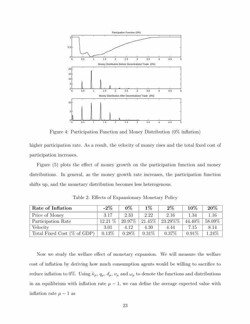
0 0.5 1 1.5 2 2.5 3 3.5 4 4.5 50

0.5

1

Paricipation Function (0%)

0 0.5 1 1.5 2 2.5 3 3.5 4 4.5 50

5

10

15

20

Money Distribution Before Decentralized Trade (0%)

0 0.5 1 1.5 2 2.5 3 3.5 4 4.5 50

5

10

Money Distribution After Decentralized Trade (0%)

Figure 4: Participation Function and Money Distribution (0% inflation)

higher participation rate. As a result, the velocity of money rises and the total fixed cost of

participation increases.

Figure (5) plots the effect of money growth on the participation function and money

distributions. In general, as the money growth rate increases, the participation function

shifts up, and the monetary distribution becomes less heterogenous.

Table 2: Effects of Expansionary Monetary Policy

Rate of Inflation -2% 0% 1% 2% 10% 20%

Price of Money 3.17 2.33 2.22 2.16 1.34 1.16Participation Rate 12.21 % 20.97% 21.45% 23.29%% 44.40% 58.09%Velocity 3.01 4.12 4.30 4.44 7.15 8.14Total Fixed Cost (% of GDP) 0.13% 0.28% 0.31% 0.37% 0.91% 1.24%

Now we study the welfare effect of monetary expansion. We will measure the welfare

cost of inflation by deriving how much consumption agents would be willing to sacrifice to

reduce inflation to 0%. Using κµ, qµ, dµ, νµ and ωµ to denote the functions and distributions

in an equilibrium with inflation rate µ − 1, we can define the average expected value with

inflation rate µ− 1 as

23

0 2 40

0.5

1

Participation Function (0%)

0 2 40

5

10

15

20

ν (0%)

0 2 40

5

10

ω (0%)

0 2 40

0.5

1

Participation Function (2%)

0 2 40

10

20

ν (2%)

0 2 40

5

10

ω (2%)

0 2 40

0.5

1

Participation Function (20%)

0 2 40

10

20

30

40

ν (20%)

0 2 40

10

20

30

ω (20%)

Figure 5: Participation and Distribution for Different Inflation Rates

24

U(µ) = (1− β)−1{σ∫ ∞

0

∫ ∞

0

[u(qµ(m, m, νµ))− qµ(m, m, νµ)] νµ(dm) νµ(dm)

−∫ ∞

0

κµ(m,ωµ)2

2κωµ(dm)}.

Then the welfare cost of having money growth rate µ relative to zero inflation is given

by 1−∆0(µ) where ∆0(µ) solves

U(µ) = (1− β)−1{σ∫ ∞

0

∫ ∞

0

[u[q0(m, m, ν0)∆0(µ)]− q0(m, m, ν0)] ν0(dm) ν0(dm)

−∫ ∞

0

κ0(m,ω0)2

2κω0(dm)}.

Distribution and welfare cost of inflation

First, to focus on a single number, given the parameter values, we find that the wel-

fare cost of 10% inflation is 1 − ∆0(10%) = 0.62% of output, as reported in Table 3. This

number is lower than the estimates of Lucas (around 1%) and Lagos and Wright (1.3%) for

the same pricing mechanism as we use in this paper. In these representative agent mod-

els, the welfare triangle provides an accurate estimate of the true welfare cost. However,

in our model, the welfare triangle over-estimates the welfare cost. The reason is that in

a heterogenous agent model an expansionary money injection by lump sum transfers re-

distributes real money balances from the rich to the poor and decreases the dispersion of

the monetary distribution. This redistribution effect may raise the average welfare in the

economy. Since the aggregate money demand curve captures only the average behavior in

an economy, the area under the money demand cannot capture this distributional effect of

inflation. Therefore, even abstracting from the hold-up problem pointed out by Lagos and

Wright, the traditional approach of estimating welfare cost using aggregate money demand

can be misleading. Note however that, inflation also affects the value of money, the terms of

trade and the participation in the centralized market, and thus in equilibrium will, generally,

25

be welfare decreasing.

Table 3: Gain from reducing inflation from 10% to 0%Model Welfare Triangle

This Model 0.62% 0.85%

Lucas (2000) 1% 1%

Lagos and Wright (2005) 1.3% 1.3%(No hold-up)

Furthermore, in our model, the welfare cost is non-linear in the size of the inflation rate,

as illustrated in Figure 6 and Table 4. The welfare cost of a one percent inflation is 0.03%

which is smaller than one-tenth of the welfare cost of a ten percent inflation. Similarly, the

welfare cost of a two percent inflation is smaller than one-fifth of a ten percent inflation.

The non-linearity in welfare cost reflects the non-linear response of participation to inflation

illustrated in Table 2. For example, a one percent inflation raises the participation rate by

1.5% and the total fixed cost by 0.03%, less than one-tenth of the corresponding numbers

for a ten percent inflation (which are 23% and 0.63% respectively). In turn, the non-linear

response of participation reflects the non-linearity of the distributional wealth effects of

inflation. As can be seen from Figure 5, as inflation increases the heterogeneity across

agents (dispersion of the money distribution) decreases, leading to smaller distributional

wealth effects of inflation. In Lagos and Wright, in the absence of such wealth effects, the

welfare cost is linear in the size of inflation. In Lucas, the welfare cost is concave in the size

of inflation.

Fixed cost and welfare cost of inflation

The non-linearity of the welfare cost depends on the size of the fixed cost, κ. Table 5

reports the welfare costs and participation rates for two percent and ten percent inflation for

different values of κ. First, the participation rate is decreasing in the size of the fixed cost

and increasing in the rate of inflation. Second, the welfare cost of a ten percent inflation

is increasing in the fixed cost while the welfare cost of a two percent inflation is decreasing

26

-0.3

-0.2

-0.1

0

0.1

0.2

0.3

0.4

0.5

0.6

0.7

-3 -2 -1 0 1 2 3 4 5 6 7 8 9 10

Inflation (%)

Wel

fare

Co

st

Figure 6: Inflation Rate and Welfare Cost

Table 4: Small inflation less costly in proportional termsWelfare Cost (WC) 1% 2% 10% WC1

WC10

WC2

WC10

This Model 0.03% 0.09% 0.62% 0.05 0.15

Lucas (2000) 0.12% 0.23% 0.87% 0.14 0.26

Lagos and Wright (2005) 0.13% 0.26% 1.32% 0.10 0.20(No hold-up)

in the fixed cost. The relative size of the welfare costs for different inflation rates depend

critically on the sensitivity of the participation rate to inflation. When the fixed cost is

relatively small (κ = 0.01), the participation rate is high and responds strongly to a two

percent inflation (from 27% to 39%), leading to a relatively large welfare cost (0.14%). When

the fixed cost is relatively large (κ = 0.1), the participation rate is low and responds less

strongly to a two percent inflation (from 7.5% to 9.0%), leading to a relatively small welfare

cost (0.06%). Again, this can be understood by the variation in the strength of the wealth

effects. As Figure 7 illustrates for the case of zero inflation, as the fixed cost increases, fewer

agents will participate in the centralized market and consequently the higher the dispersion

of the money distribution. This implies that for a higher fixed cost the distributional wealth

effects will be stronger for any given rate of inflation.

27

Table 5: Fixed cost and welfare cost of inflationµ Welfare Cost Part. Rate

κ=0.01 0% 0 27%2% 0.1404 39%10% 0.4089 64%

( WC2

WC10= 0.34)

κ=0.02 0% 0 21%2% 0.0854 23%10% 0.6226 44%

( WC2

WC10= 0.14)

κ=0.1 0% 0 8%2% 0.0610 9%10% 0.7324 15%

( WC2

WC10= 0.08)

0 2 40

0.5

1

Part. Fn. ( κ = 0.01)

0 2 40

5

10

15

20

ν ( κ = 0.01)

0 2 40

0.5

1

Part. Fn. ( κ = 0.1)

0 2 40

5

10

ν ( κ = 0.1)

Figure 7: Fixed Cost, Participation Function, and Heterogeneity (µ = 0)

A policy implication is that, as the fixed cost decreases overtime (due to financial devel-

opment, for example), the welfare cost of inflation will be affected. However, the impact on

welfare costs of different inflation rates can be completely different both quantitatively and

28

qualitatively. In these examples, the welfare cost goes down for high inflation but goes up

for low inflation. It would be misleading to use the welfare cost of a ten percent inflation

to extrapolate that of a smaller inflation. This considerations are particularly important

given that the data suggest there might have been important structural changes to the U.S.

aggregate money demand in recent decades. In particular, because such changes might be

associated with financial development. Figure 8 illustrates breaks the data points by decade.

As can be seen, the aggregate money demand has become flatter overtime, implying a lower

interest-elasticity of money demand. This implies that the welfare costs of say, 10% inflation,

for the U.S. economy might actually be smaller than our estimate.

0

0.1

0.2

0.3

0.4

0.5

0.6

0 0.05 0.1 0.15 0.2

Nominal Interest Rate

M1/

GD

P

1900-19601961-19801981-2000

Figure 8: U.S. Money Demand Overtime

6 The Canadian Economy

In this section, we redo the above exercise for the Canadian economy. We pick the parameter

values to match the empirical money demand for Canada: σ = 0.5, β = 0.9992, η = 0.99,

29

0

0.05

0.1

0.15

0.2

0.25

0.3

0 5 10 15 20 25 30

Nominal Interest Rate

M1/

GD

P

Model

Data (1934-59)

Data (1960-99)

Figure 9: Model vs. Canadian Data

b = 0.0001, κ = 0.04.20 Figure 9 plots the Canadian time-series data (1933-99) and the

money demand curve implied by the model. The model fits the data points after 1960 better

than those before 1960. This might be due to the revision of the Nominal GDP series starting

in 1961. But we do not discount the possibility that there was structural shifts of the money

demand curve over time. However, for the inflation region of our interest (that is, interest

rate over four percent), the demand curve implied by the model does fit the data well.

Table 6 reports the effects of expansionary monetary policy in this economy. The qual-

itative results are similar to those in the previous section: inflation increases the price of

money, the participation rate, the velocity and the total fixed cost. The welfare cost of a

ten percent inflation is 0.2%. Again, this is lower than the welfare triangle which is 0.34%.

It is worthwhile noticing that the welfare costs of a 10% inflation for the Canadian economy

is one third of that of the U.S. economy. This finding is consistent with previous estimates

20We use M1 plus bank non-personal notice chequable deposit (post 1968) as the monetary aggregate andthe 90 days T-bill auction average yield as the nominal interest rate. M1 estimates prior to 1953 are takenfrom Metcalf, Redish et al. (1998), post 1953 are taken from CANSIM series V372000. Nominal GDP isobtained from CANSIM series V500633(34-60) and V646937(after 61). The definitions used in the latterseries are not consistent and might explain the difficulty of the model in matching the period pre-1961.

30

Table 6: Effects of Expansionary Monetary PolicyRate of Inflation 0% 2% 10%

Price of Money 3.62 3.15 2.23Participation Rate 13% 17% 26%Velocity 7.25 8.50 11.61Total Fixed Cost (% of GDP) 0.12% 0.17% 0.32%Welfare Cost (% of C) 0% 0.08% 0.20%Welfare Triangle 0% 0.05% 0.34%

of the welfare costs of inflation for both economies using a representative agent models and

is a reflection of the lower interest-elasticity of the Canadian money demand implied by the

data. If one takes into account the recent possible structural changes to the U.S. aggregate

money demand such difference might decrease or vanish. Also, the welfare cost is a non-

linear function of the inflation rate. In this case, the welfare cost of a two percent inflation

is larger than one-fifth of a ten percent inflation.

7 Discussion and Conclusion

This paper develops a micro-founded model to study the effect of inflation on distribution

and welfare. By modeling inflation and liquidity market working as alternative insurance

mechanisms, this paper illustrates the following findings.

First, distributional effects matter for the welfare. Even without the hold-up problem,

measuring welfare cost by aggregate demand function can be misleading. This finding sug-

gests that, knowing the aggregate money demand curve is not sufficient, we need to have the

information on the distribution to have an accurate estimate of the welfare effects of infla-

tion. Second, the welfare effect of inflation is nonlinear in the inflation rate. Measuring the

welfare cost of inflation by extrapolating high inflation data to unobservable low inflation re-

gion can be misleading. Third, the welfare cost of inflation depends on the participation cost

of liquidity market. Financial development can affect the welfare cost of different inflation

rates differently.

31

In terms of policy implications for Canada, our findings suggest that the welfare cost

of low inflation (e.g., 2%) is relatively small. If transition costs are non-trivial, then there

might be no welfare gains of reducing the current inflation target further. Also, if there are

additional costs of reducing inflation not captured by the model, there might be no gains of

reducing the current inflation target.

By focusing on the steady state analysis, we cannot capture the full welfare effect of

adjusting inflation rates. To be able to properly measure the potential gain/loss of changing

inflation targets one needs to take into consideration the transitional effects and to explicitly

solve for the short-run dynamics out of steady state. This interesting but challenging task

will be delegated to future research.

32

References

Alvarez, Fernando, Andrew Atkeson and Chris Edmond. (2003). “On the Sluggish

Response of Prices to Money in an Inventory-Theoretic Model of Money Demand,” NBER

Working Paper No. w10016.

Alvarez, Fernando, Andrew Atkeson and Patrick J. Kehoe.(2002). “Money, Interest

Rates, and Exchange Rate, with Endogeneously Segmented Markets”, Journal of Political

Economy 110, 73-112.

Bailey, Martin J. (1956). “The Welfare Cost of Inflationary Finance,” Journal of Political

Economy 64, 93-110.

Baumol, William J. (1952). “The Transactions Demand for Cash: An Inventory Theo-

retical Approach,” Quarterly Journal of Economics 66, 545-56.

Berentsen, Aleksander, Gabriele Camera and Christopher Waller. (2005). “The Dis-

tribution Of Money Balances And The Nonneutrality Of Money”, International Economic

Review 46, 465-87.

Chiu, Jonathan. (2005). “Endogenously Segmented Asset Market in an Inventory The-

oretic Model of Money Demand”, mimeo, The University of Western Ontario.

Chiu, Jonathan and Miguel Molico. (2006). “Endogenous Asset Market Participation

and Random Matching in an Inventory Model of Money Demand”, manuscript.

Deviatov, Alexei and Neil Wallace. (2001). “Another Example in Which Lump-sum

Money Creation Is Beneficial,” Advances in Macroeconomics 1, Article 1.

Ennis, Huberto. (2005). “Avoiding the Inflation Tax”, Working Paper, Federal Reserve

Bank of Richmond Working Paper 05-10.

Friedman, Milton. (1969). ‘The Optimum Quantity of Money and Other Essays. Chicago:

Aldine.

Grossman, Sanford J, and Weiss, Laurence. (1983). “A Transactions-Based Model of the

Monetary Transmission Mechanism”, American Economic Review 73, 871-80.

Imrohoroglu, Ayse. (1992). “The Welfare Cost of Inflation Under Imperfect Insurance,”

33

Journal of Economic Dynamics and Control 16, 79-91.

Jovanovic, Boyan. (1982). “Inflation and Welfare in the Steady State,” Journal of

Political Economy 90, 561-77.

Khan, Aubhik and Julia Thomas. (2005). “Inflation and Interest Rates with Endogenous

Market Segmentation”, manuscript.

Lagos, Ricardo and Randall Wright. (2005). “A United Framework for Monetary Theory

and Policy Analysis”, Journal of Political Economy 113, 463-484.

Levine, David. (1991). “Asset Trading Mechanisms and Expansionary Policy,” Journal

of Economic Theory 54, 148-64.

Lucas, Robert. (2000). “Inflation and Welfare”, Econometrica 68, p. 247-274.

Metcalf, Cherie, Angela Redish, and Ronald Shearer. (1998). “New Estimates of the

Canadian Money Stock, 1987-1967,” The Canadian Journal of Economics 31, 104-124.

Molico, Miguel. (2006). “The Distribution of Money and Prices in Search Equilibrium”,

International Economic Review 47, 701-722.

Romer, David. (1986). “A Simple General Equilibrium Version of the Baumol-TobinModel,”

Quarterly Journal of Economics 101, 66385.

Serletis, Apostolos, and Kazem Yavari. (2004). “The Welfare Cost of Inflation in Canada

and the United States,” Economic Letters 84, 199-204.

Tobin, James. (1956). “The Interest-Elasticity of Transactions Demand for Money,”

Review of Economics and Statistics 38, 241-47.

Telyukova, I. and R. Wright. (2005). “A Model of Money and Credit, with Application

to the Credit Card Debt Puzzle ”, University of Pennsylvania working paper.

Williamson, Stephen. (2006). “Search, Limited Participation, and Monetary Policy”,

International Economic Review 47, 107-128.

34