1

Literature Review and Assessment of theEnvironmental Risks Associated With the

Use of ACQ Treated Wood Productsin Aquatic Environments

Prepared for:

Western Wood Preservers Institute7017 NE Highway 99, Suite 108

Vancouver, WA 98665

Prepared by:

Kenneth M. Brooks, Ph.D.

Aquatic Environmental Sciences644 Old Eaglemount RoadPort Townsend, WA 98368

December 5, 2001

Table of Contents Page

Introduction 1

Background levels and sources of DDAC and copper in aquatic environments. 1

Cycling and fate of DDAC and copper in aquatic environments. 3

Bioaccumulation of DDAC and copper in aquatic environments. 6

Toxicity of DDAC and copper dissolved in the water column to aquatic fauna and flora. 8

Regulatory levels defining water quality criteria 14

Toxicity to aquatic organisms associated with sedimented copper 15

Regulatory standards for copper with respect to marine and freshwater sediments. 23

Toxicity to aquatic fauna and flora associated with didecyldimethylammonium chloride(DDAC) dissolved in the water column 27

Recommended water column benchmarks for DDAC 30

Toxicity to aquatic fauna and flora associated with sedimented DDAC 31

Recommended sediment benchmark for DDAC 32

Summary statement regarding recommended benchmarks for dissolved and sedimented Copper and DDAC for use in this risk assessment. 32

Anticipated environmental impacts resulting from the use of 0.4 pcf ACQ treated wood in aquatic environments. 34

Leaching of DDAC and copper from ACQ treated wood. 34

Factors affecting ACQ-B copper leaching rates 35

Environmental factor affecting the loss of DDAC from ACQ-B preserved wood 39

Preservative loss from overhead structures. 42

Table of contents - continued

Risk Assessment Part I. Anticipated environmental levels of copper and DDAC Resulting from the use of 0.4 pcf ACQ-B treated wood in freshwater environments Dominated by steady state currents (streams and rivers) 43

Water column concentrations of DDAC and copper lost from piling in fresh or Brackish water dominated by steady state currents. 44

2

Deposition rates of copper and DDAC to sediments in freshwater streams and rivers 44

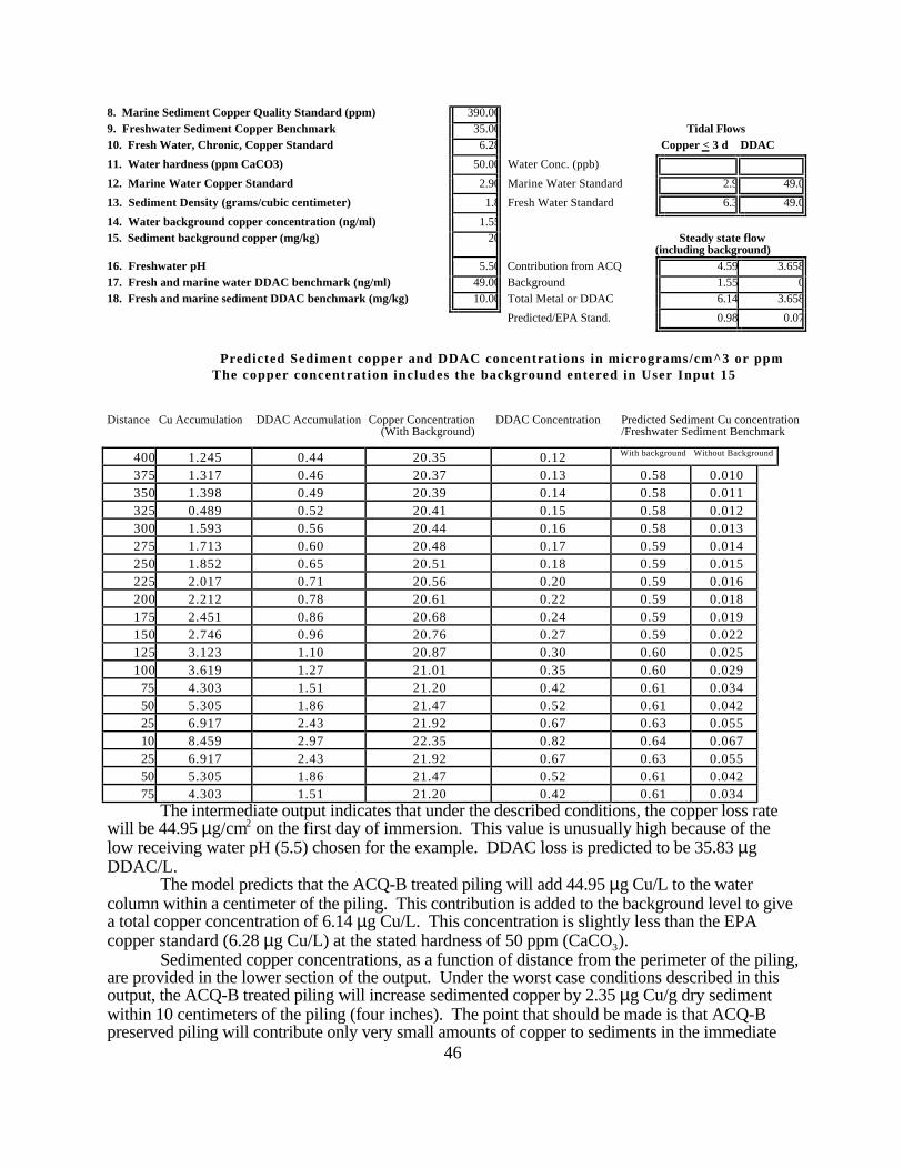
Accumulation of copper in freshwater sediments 46

Accumulation of DDAC in sediments 47

Predictive computer model for 0.4 pcf ACQ-B preserved wood used in Freshwater environments with steady state current speeds. 47

ACQ-B projects proposed for small, closed, bodies of water such as ponds 52

Summary for the use of 0.4 pcf ACQ-B preserved southern yellow pine inFreshwater and evaluation of generalized risks. 53

Risk Assessment Part II. Anticipated environmental levels of copper resulting from the use of 0.4 pcf ACQ-B treated piling used in constructing large surface area projects, such as bulkheads (ACQbrisk.xls) 56

Water column concentrations of copper associated with large surface areaprojects such as bulkheads treated with ACQ preservative. 58

Sediment concentration of copper associated with the use of 0.4 pcf ACQ-BTreated lumber in bulkheads. 59

Predicted concentration of copper in the water column and sediments associatedwith the use of 0.4 pcf ACQ-B treated lumber used to construct bulkheadsand other large surface area structures in freshwater environmentsincluding those influenced by tidal currents 60

Generalized risks associated with the use of ACQ-B treated wood used in theconstruction of freshwater bulkheads 61

Table of contents - continued

Risk Assessment Part III. Environmental risks associated with the use of 0.4 pcf ACQ-B preserved piling in environments influenced by tidal currents(ACQprisk.xls) 63

Sedimentation of adsorbed metals 63

Risk assessment model for piling used in freshwater areas influenced bytidal currents. 66

Model output. Water column copper concentrations associated with ACQ-BTreated piling installed in areas influenced by tidal currents. 69

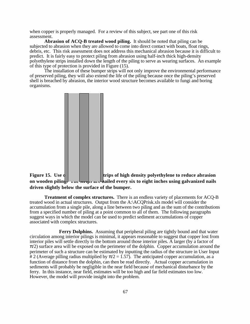
Abrasion of ACQ-B treated wood piling 74

Treatment of complex structures 74

3

General recommendations for the use of 0.4 pcf ACQ-B preserved southern yellowPine or hem-fir piling used in freshwater environments influenced by tidalCurrents. 75

Summary and Conclusions 76

References 78

List of Tables

Table Page

1. Summary of environmental fate properties of DDAC. 5

2. Metal concentration factors (dimensionless) for submerged aquatic plants. From Rai et al. (1995). 7

3. Mean number of total macroinvertebrates per sample (M), mean percentage contribution of selected major taxa to the total macroinvertebrate fauna (P), and

number of species (S) observed by Gower et al. (1994) as a function of water columnlevels of copper expressed as proportional increases in the U.S. EPA freshwatercopper criteria at the observed level of hardness. 10

4. Water chemistry at sample stations 1 (upstream), 3 (in roast pits) and 4 (immediately downstream from roast pits) in the study of Rutherford and Mellow (1994). 11

5. Selected macro-invertebrate taxa with significant sensitivity or tolerance to high copperlevels at sample stations 1 (upstream), 3 (in roast pits) and 4 (immediately

downstream from roast pits) in the study of Rutherford and Mellow (1994). Taxa exhibiting moderate to strong copper tolerance are bolded. Dissolved

4

copper concentrations are provided in parentheses after each stationnumber (µg/L) 12

6. Total Copper Toxicity Measured in Controlled Bioassays. Values are EC50 or LC50 in ppb 14

7. Summary of copper concentrations in the water column and sediments of reference Loken Lake (LOK) and impacted Manitouwadge Lake (MAN). Significant macro-invertebrate data are included to indicated faunal response. All values are in mg/kg. Data are taken from Munkittrick et al. (1991). 18

8. Comparison of metal levels and infauna at four lakes downstream from the Con Minein the Canadian subarctic. All metal concentrations are in mg/kg (dry sedimentweight). 19

9. Heavy metal contents of sediments and of larvae of Baetis rhodani collected from six rivers in the German Federal Republic. Sediment Bioconcentration Factors are calculated for each river. All values are in mg Cu/kg dry sediment. 20

List of Tables – continued

10. Summary of sediment types, test conditions and results of copper spiked sediment bioassays reported by Cairns et al. (1984). 21

11. Background freshwater sediment copper levels reviewed in this assessment. All values are presented in mg Cu/g dry sediment. 21

12. Summary of the tolerance of various freshwater taxa to sedimented copper 22

13. Summary of jurisdictional screening level benchmarks for screening hazardous wastesites for contaminants of concern 25

14. Recommended benchmarks for assessing the environmental risks associated with sedimented copper lost from pressure treated wood. 26

15. Summary of conventional benchmarks for copper in freshwater (µg/L). The data are from Suter and Tsao (1996). The Environmental Protection Agency National Water Quality Criteria for copper was computed at a hardness of 100 mg (CaCO3) /L. 27

16. Summary of DDAC LC50 data for aquatic species from Brooks et al. (1996). All values are in µg active ingredient/L 28

5

17. Summary of no-observed effect levels (NOEL) measured for DDAC 29

18. The effect of DOC on toxicity of the antisapstain chemical, DDAC, to fathead minnows in a 96 hr. static renewal acute toxicity test (from Brooks et al., 1996) 30

19. Water and sediment copper and DDAC benchmarks against which to assess the environmentalsuitability of ACQ-B preserved wood used in aquatic environments 33

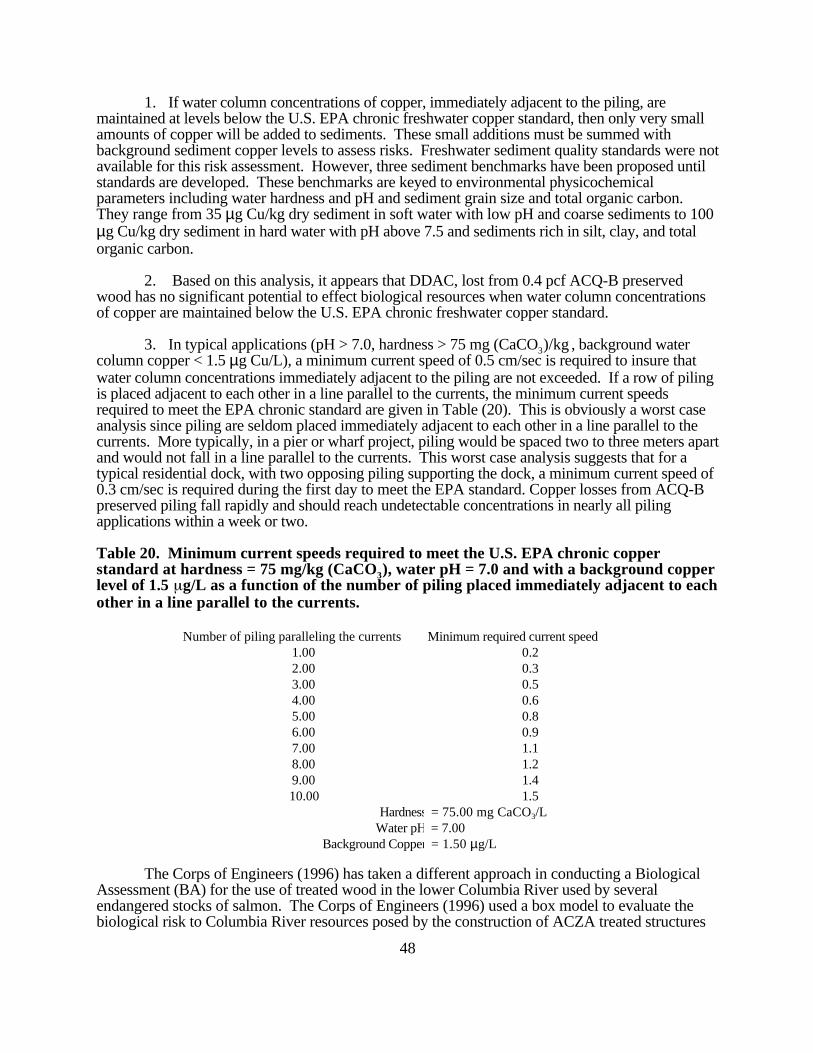
20. Minimum current speeds required to meet the U.S. EPA chronic copper standard at hardness = 75 mg/kg (CaCO3), water pH = 7.0 and with a background copper level of 1.5 µg/L as a function of the number of piling placed immediately adjacent to each other in a line parallel to the currents 54

List of Tables – continued

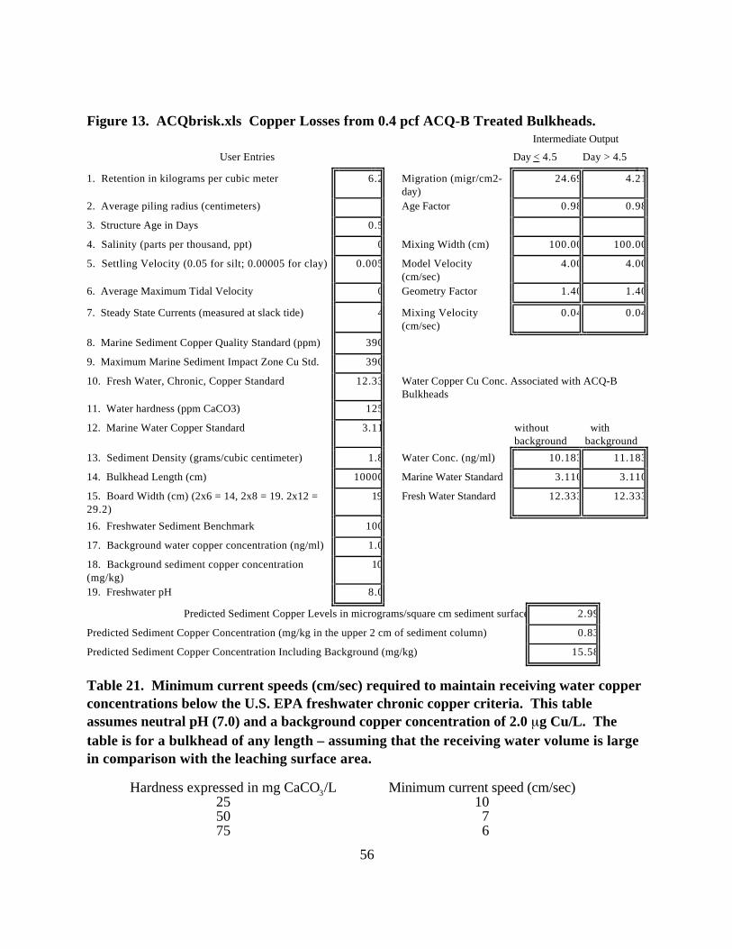
21. Minimum current speeds (cm/sec) required to maintain receiving water copper concentrations below the U.S. EPA freshwater chronic copper criteria. Thistable assumes neutral pH (7.0) and a background copper concentration of 2.0 µg Cu/L. The table is for a bulkhead of any length – assuming that thereceiving water volume is large in comparison with the leaching surface area. 62

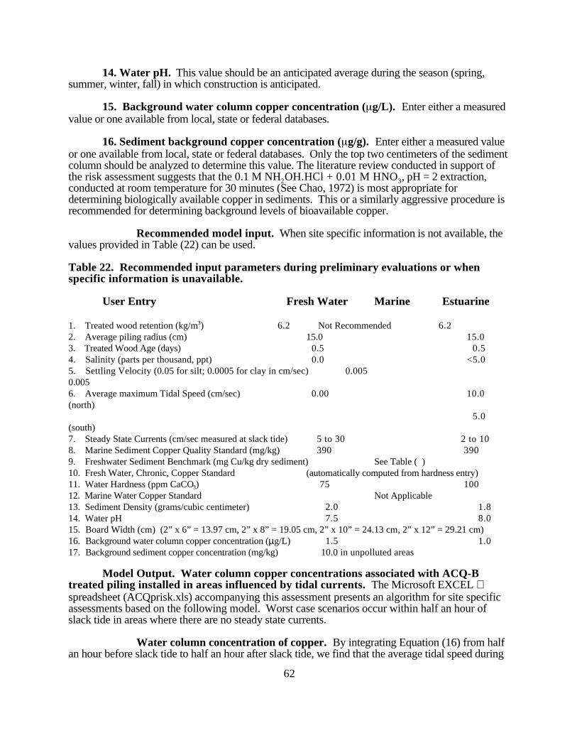
22. Recommended input parameters during preliminary evaluations or when specific information is unavailable 69

23. Minimum required values of the model velocity required at a range of hardness values(mg CaCO3/L) to maintain copper concentrations less than the U.S. EPA chronicfreshwater copper criterion. These values are appropriate for a single piling, placedin water with pH = 7.0 and a background copper concentration of 1.0 µg/L

75

6

7

List of FiguresPage

1. U.S. EPA chronic and acute copper criteria for freshwater. The copper standard is presented in µg/L and hardness values in mg (CaCO3)/L. 15

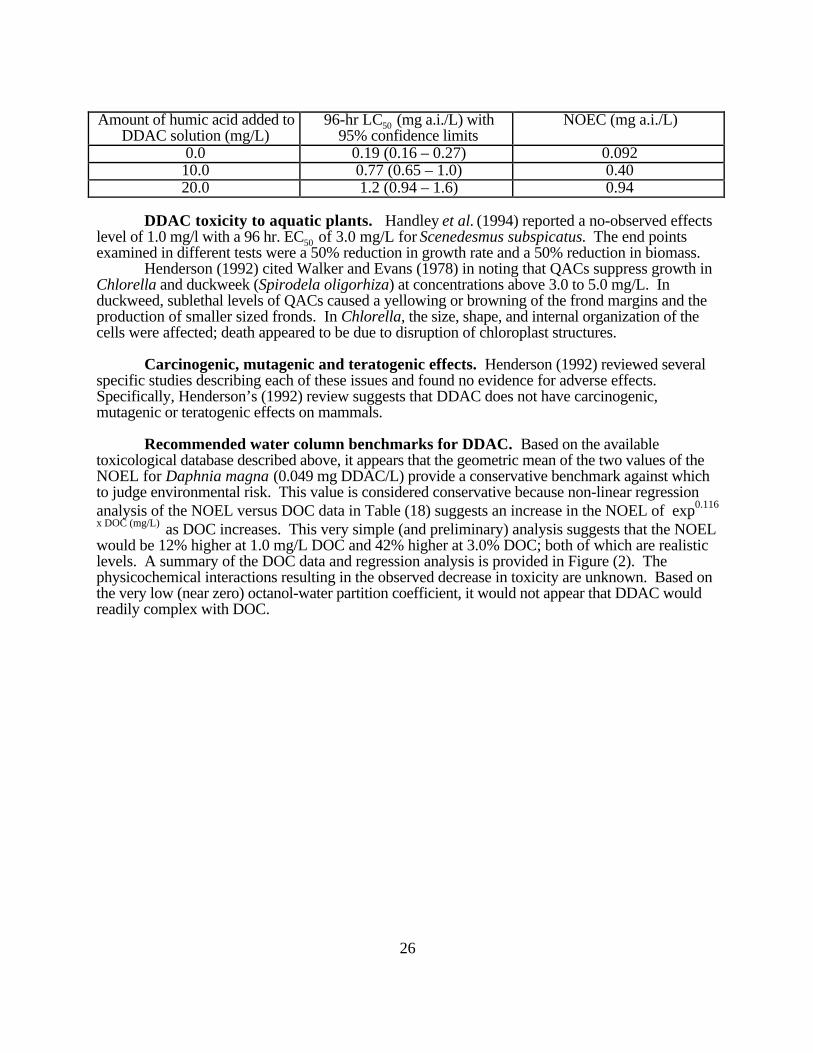
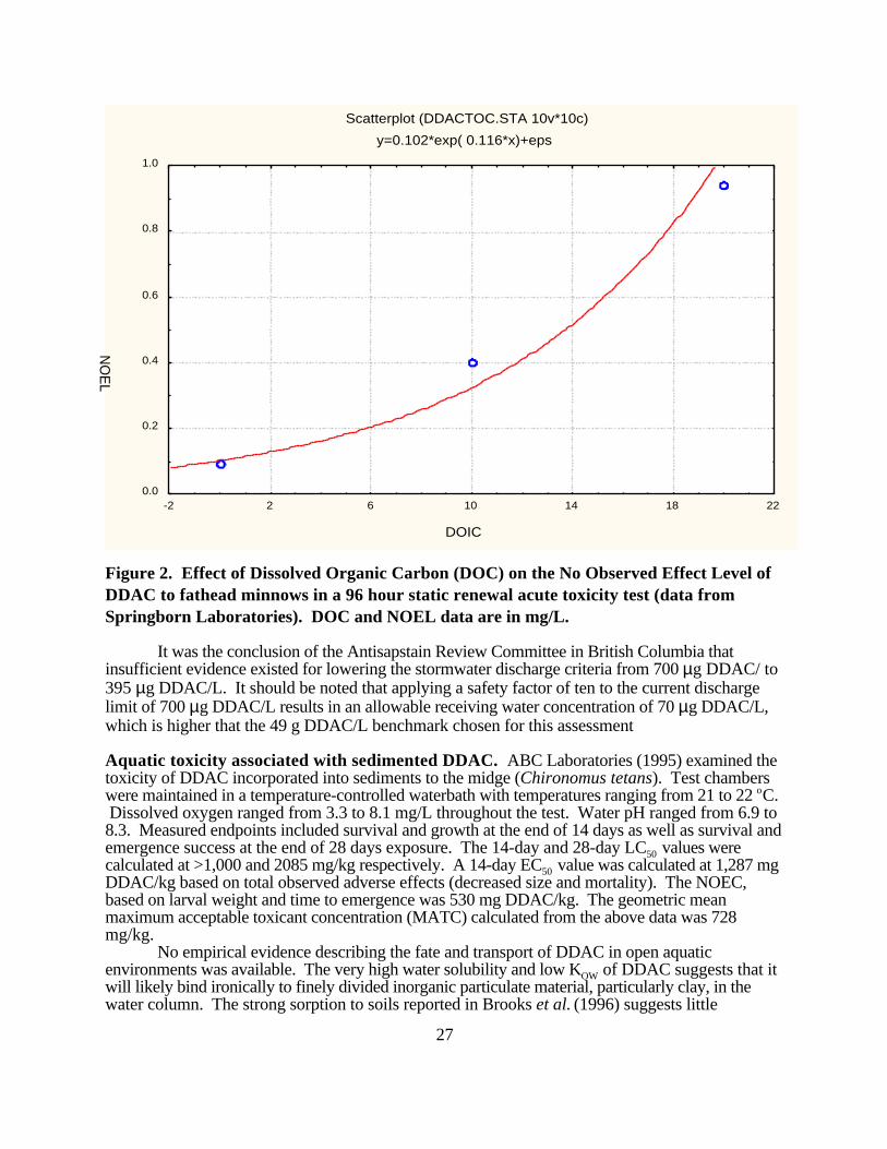
2. Effect of Dissolved Organic Carbon (DOC) on the No Observed Effect Level of DDAC to fathead minnows in a 96 hour static renewal acute toxicity test (data from Springborn Laboratories). DOC and NOEL data are in mg/L 31

3. Copper loss as a function of time (µg/cm2/day) from southern yellow pine poles, treated to 0.4 pcf with ACQ-B preservative and leached into 10 to 12 liters of

distilled water amended to a pH of 5.0, 6.5 or 8.0 and in saltwater (30 ppm) at pH8.0. Data from Jin (1997). 36

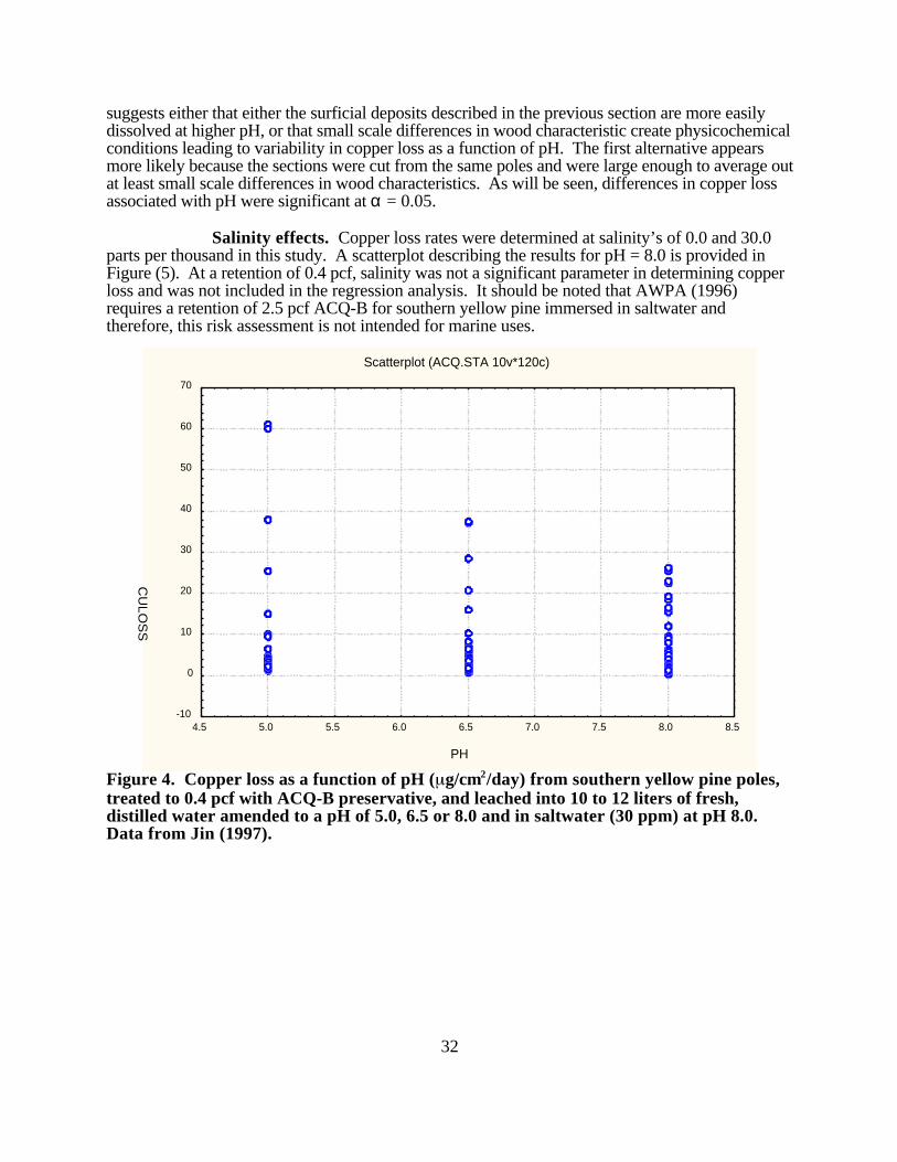
4. Copper loss as a function of pH (µg/cm2/day) from southern yellow pine poles, treated to 0.4 pcf with ACQ-B preservative, and leached into 10 to 12 liters of

fresh, distilled water amended to a pH of 5.0, 6.5 or 8.0 and in saltwater (30 ppm) atpH 8.0. Data from Jin (1997). 37

5. Copper loss (µg/cm2/day) from southern yellow pine poles, treated to 0.4 pcf with ACQ-B preservative and leached into either freshwater (salinity = 0.0)

or seawater (salinity = 30 g/L). Data from Jin (1997) 37

6. Copper loss (µg/cm2/day) as a function of time and pH from southern yellow pine poles, treated to 0.4 pcf with ACQ-B preservative and leached into freshwater at pH values of 5.0, 6.5 and 8.0. Data from Jin (1997) 38

7. DDAC losses from 0.4 pcf ACQ-B treated southern yellow pine as a function of time at pH = 5.0, 6.5 and 8.0 and at salinities of 0.0 and 30.00 ppt. Data from Jin (1997) 39

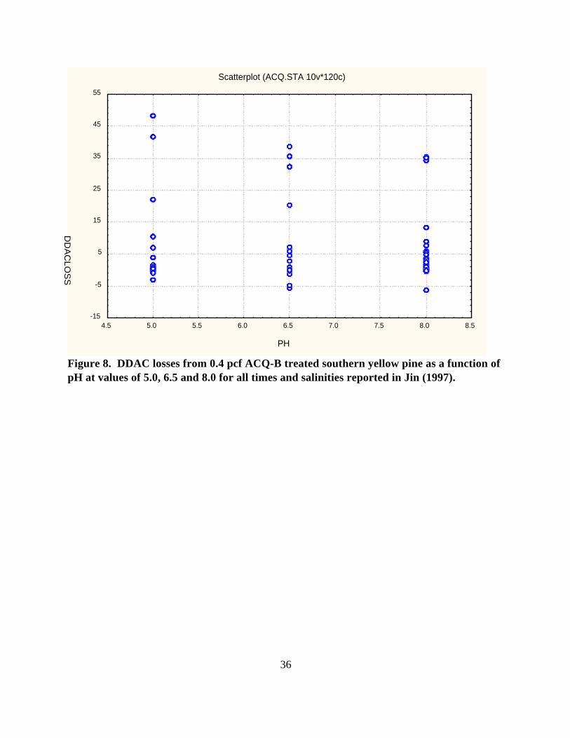
8. DDAC losses from 0.4 pcf ACQ-B treated southern yellow pine as a function of pH at values of 5.0, 6.5 and 8.0 for all times and salinities reported in Jin (1997) 40

9. DDAC losses from 0.4 pcf ACQ-B treated southern yellow pine as a function of salinity at a pH value of 8.0 for all times reported in Jin (1997). 41

10. Summary of predicted copper and DDAC losses in µg/cm2/day from 0.4 pcf, ACQ-B treated southern yellow pine in receiving water with a pH of 7.0 42

List of Figures - continued

8

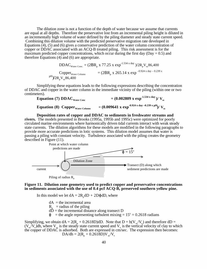
11. Dilution zone geometry used to predict copper and preservative concentrations insediments associated with the use of 0.4 pcf ACQ-B, preserved southern yellow pine

45

12. Copper and DDAC Accumulation in Water and Sediments Associated with the use of ACQ Treated Piling 51

13. ACQbrisk.xls Copper Losses from 0.4 pcf ACQ-B Treated Bulkheads 62

14. Tabular input and output from the Microsoft EXCEL spreadsheet A:\ACQPrisk 73

15. Use of half-inch thick strips of high density polyethylene to reduce abrasion on wooden piling. The strips are nailed every six to eight inches using galvanized nails driven slightlybelow the surface of the bumper 74

Literature Review and Assessment of the Environmental RisksAssociated With The Use Of ACQ Treated Wood Products in Aquatic Environments

Introduction. Ammoniacal copper quat (ACQ-B) is a wood preservative, developed and patentedin Canada (Findlay and Richardson, 1983; 1990), containing between 62 and 71 percent copperoxide (CuO) and between 29 and 38 percent quat as didecyldimethylammonium chloride (DDAC). These active ingredients are dissolved in a water carrier to which is added ammonia (NH3), equal inweight to the copper oxide in the preservative and carbonate equal to 0.65 times the amount ofcopper oxide.

The quaternary ammonium compound in ACQ-B promotes fixation in wood through ionexchange with anionic active sites and through other adsorption mechanisms at higher quatconcentrations (Archer et al. 1992). Quat is fixed predominantly onto lignin, although interactionwith holocellulose also occurs. Copper is fixed in wood through ion exchange reactions betweencupriammonium ions and acidic functional groups such as the carboxylic acid groups of lignin andhemicellulose. Copper complexes with cellulose through hydrogen bonding with hydroxyl oramine nitrogen groups, or through replacement of an ammonia group from the cupriammonium ionwith the hydroxyl ion of cellulose. Copper also forms insoluble copper carbonate salts resultingfrom the loss of ammonia during drying (Chen, 1994).

Copper does not generally constitute a human health risk. Neither copper, nor DDAC areexpected to have carcinogenic, teratogenic or mutagenic effects. However, low concentrations ofboth copper in certain ionic forms and DDAC can be toxic to aquatic fauna and flora.

Several reviews assessing the environmental risks associated with treated wood have beencompiled by Hartford (1976), Konasewich and Henning (1988), Stranks (1976), Ruddick andRuddick (1992) and the U.S. Department of Agriculture (1980). The conclusion reached in thesepapers is that the use of treated wood causes no significant hazard to the environment. However,none of these reviews considered ACQ and all suffer from lack of quantitative analysis, leavingsome doubt about the risks associated with using treated wood in aquatic environments. Brooks(1995, 1996, 1997a, 1997b, 1997c) has previously published a series of risk assessment guides forCCA-C, ACZA and creosote treated wood used in freshwater and marine environments. This riskassessment is for wood treated with ACQ-B to a retention of 0.40 pounds per cubic foot (6.2 kg-m-

3) in the treated zone. This retention is prescribed by AWPA (1996) for treatment of southern pine,coastal Douglas-fir, sitka spruce, western hemlock and hem-fir used in ground and/or fresh watercontact. This risk assessment is not intended formarine applications where salinity exceeds two parts per thousand for extended periods of time.

Background Levels and Sources of Copper and DDAC in Aquatic Environments.

Water column levels of copper. Copper is a naturally occurring element found in allaquatic systems. At low levels it is considered a micronutrient essential to the proper functioning ofplants and animals. Copper levels of 1 - 10 ppb were reported by Boyle (1979) from unpollutedwaters of the United States. However, concentrations downstream of municipal and industrialoutfalls may be much higher (Hutchinson, 1979). Background levels of one to three µg Cu/L wereobserved by USGS between 1995 and 1997 in Columbia River water with a mean of 2.00 µg Cu/L. The lower Columbia River carries approximately 650 kilograms of copper past any point every dayat a concentration of 2.0 µg/L.

Sediment levels of copper. Background levels of copper in lower Columbia Riversediments ranged between 18 and 66 mg/kg (Siipola, 1991). Similarly, Tetra Tech (1994) observedsediment copper concentrations ranging from 19.3 to 49.9 with a median concentration of 27.6mg/kg in the Columbia River. Munkittrick et al. (1991) reported reference area sediment copperconcentrations of four to 23 mg/kg in northern Ontario. Cairns et al. (1984) reported copper levelsof 59 mg/kg in control sediments from the Tualatin River, Oregon and 210 mg/kg in controlsediments from Soap Creek Pond at Oregon State University.

2

Crocket and Kabir (1981) observed widespread increases in copper concentrations in theupper five centimeters of sediments from the Sudbury-Temagami area in Ontario to ca. 50 to 75mgCu/kg dry sediment weight. They associated these increases to atmospheric deposition from thenearby Sudbury industrial complex. Hupp et al. (1993) observed sedimented copperconcentrations of three to 24 mg/kg along the Chickahominy River in Virginia. Highest levels ofsedimented copper were associated with the most urban-industrial part of the river basin. Their dataindicated that 17,170,000 kilograms of sediment was deposited in wetlands along this river eachyear and that the annual deposition of copper to these sediments was 176 kilograms.Larsen (1983)estimated a mean annual atmospheric copper deposition rate of 1.81 to 2.77 mg/m2 at four Danishlakes. Larsen (1983) cites Hovmand’s (1979) finding that ten to 60 percent of the heavy metalloading to the Baltic Sea is from atmospheric deposition and measured copper concentrations inrainwater that varied between 1.79 and 2.49 µg/L.

These data suggest that background levels of sedimented copper can vary significantly atsites unaffected by identifiable sources of pollution. Background levels appear to vary from lessthan ten to perhaps 70 to 200 µg Cu/kg dry sediment weight. It also appears reasonable toconclude that atmospheric deposition is a significant source of copper over large areas.

Didecyldimethylammonium chloride (DDAC) is a member of the quaternaryammonium compounds (QAC). QACs were first synthesized in the late 1800’s and theirbactericidal properties were reported about two decades later. These compounds are well known fortheir germicidal, fungicidal, and algicidal properties when the alkyl fractions contain fewer thaneight to 14 carbon atoms. Formulations containing between 0.01 and 1.0% QACs are usedextensively as antiseptics, bactericides, fungicides, sanitizers and deodorants. QACs are alsopopular disinfectants for utensils, containers, and other instruments used in restaurants dairies, foodplants, laundries, and operating rooms (Gosselin et al., 1984).

Quatenary ammonia compounds (QACs) with carbon chain lengths exceeding 14 are usedextensively as softener’s in laundry applications. Huber (1984) reports that 39,000 tons ofquaternary ammonium compounds were marketed in the USA in 1978 for this purpose. Therefore,there is considerable opportunity for this class of compounds to enter aquatic ecosystems. Huber(1984) reported 19 µg/L DSDMAC and 5 to 20 µg/L DSBAS in waters of the Main River, nearFrankfurt, West Germany. The point is that this general class of compounds is used extensively inmodern society and they are finding their way into aquatic ecosystems in detectable amounts. Therefore, their ecological effects are of interest and they require management to insure that adverseeffects are not associated with their use.

Didecyldimethylammonium chloride (DDAC) is not known to occur naturally. Hence, allDDAC found in aquatic environments results from spills and wastewater or stormwater dischargesfrom commercial facilities using the chemical (antisapstain compounds and wood preservativesapplied to lumber, laundry and residential waste water, restaurants, hospitals, etc.). As will beshown, DDAC is highly water-soluble with an octanol/water partition coefficient reported near zero. Therefore it has little propensity to accumulate in sediments, to bioconcentrate in aquaticorganisms, or to biomagnify in food chains. No information describing detectable levels of DDACin aquatic environments (sediments or water) was obtained.

Cycling and Fate of Copper and DDAC in Aquatic Environments

Copper. Copper occurs in soft natural waters primarily as the divalent cupric ion. It maybe found as a free ion or complexed with humic acids, carbonate, or other inorganic and organicmolecules in water of increasing hardness. Copper is an essential element in the normalmetabolism of both plants and animals. Therefore, a significant portion of the copper found in bothfresh and marine systems may be taken up by the biota. The ultimate fate of much of this copper issedimentation.

3

Harrison, et al. (1987) found very low copper levels (< 12 ppb) in sandy substratesassociated with power plant effluents and suggested that the lack of organic matter in thesesediments was responsible for the low copper content. In contrast, Kerrison et al. (1988) foundthat copper added to enclosures placed in a shallow fertile lake rapidly became associated withsuspended particulate material in the water column. The environment in which these experimentswere conducted suggests that the particulate matter consisted of particulate organic matter (POM)and/or particulate inorganic matter (PIM) which would most likely be in the form of clay particles.Little suspended silt would be anticipated in a shallow freshwater lake.

Clarke (1974) noted that iron sulfide will render copper insoluble in anaerobic sediments. This report suggests that copper accumulation in sediments is highly influenced by sedimentchemistry and physical characteristics. Fine sediments, coupled with poor water circulation couldbe expected to accumulate more copper than coarse sediments in highly oxygenated areas. Copperaccumulations in fine grained, anaerobic sediments are probably not biologically available, thusthese environments may serve as an important mechanism for the removal of excess copper fromaquatic environments.

Schmidt (1978) reported that average copper levels in open ocean water was ca. 1.15 µg/Lwith a rather broad range of 0.06 to 6.7 µg/L. Copper levels in coastal and nearshore water werehigher with a mean of 2.0 µg/L. In nearshore water, more copper was found bound to particulatematerial (50.7%) than is found complexed in a dissolved form (49.3%). In open-sea samples,copper was partitioned between particulate (34.8%) and dissolved (65.2%) compartments. Schmidt(1978) reported that much of the copper in nearshore and offshore waters was associated withparticulate material and that approximately 10% was adsorbed to clay. The average concentration ofcopper in suspended particulate material in the ocean was 109 µg/g with a range of 52 to 202. Schmidt (1978) noted that these levels were higher than those found in most nearshore sediments. He suggested that fine suspended particulates, rich in copper, are probably an important media fortransporting continentally derived copper from the near shore to pelagic areas where the finalrepository for copper is likely in deep ocean sediments.

Cycling of copper from sediments as a function of the REDOX potential. Lu andChen (1977) examined the release of copper from sediments as a function of sediment grain sizeand oxygen availability. Sediment grain size was not a factor in the amount of copper released tothe overlying water column. Three oxidizing conditions were examined (oxidizing, 5 to 8 ppmdissolved oxygen; slightly oxidizing, < 1 ppm dissolved oxygen; and reducing, S(-II)T = 15 to 30ppm). Small amounts of bound copper were released from sediments into the overlying water inreducing and slightly oxidizing environments (0.2 to 0.5 ppb). Copper releases in the oxidizingenvironment resulted in significantly higher interfacial seawater concentrations (3.2 ppb). Thiseffect was slightly more pronounced in the coarsest sediment tested (silty-sand sediment). Thesedata imply higher copper releases from sediments in aerobic (biologically healthy) environments. There are two ways to look at these results:

First, in coarse grained, highly oxygenated sediments, bound copper is more easily lost tothe water column and dispersed over greater distances. Eventually, most of the copper deposited inareas with anaerobic sediments, where it is buried and incorporated into the lithosphere. Theseanaerobic sediments support reduced infaunal and epifaunal communities of organisms. As aresult, we might expect reduced environmental impacts from copper incorporated into thesesediments.

Alternatively, in enclosed bodies of water with coarse grained, aerobic, sediments, this studysuggests that copper will not be as tightly bound to the sediments and will cycle between sedimentsand interstitial and surficial waters where it is bioavailable. No data was provided on the copperspecies released from the sediments and therefore it is difficult to assess the toxicity of the releasedcopper in this scenario. However, the biological effects associated with copper in thisenvironmental would certainly be more significant than that associated with depauperate, anaerobicsediments.

4

The work of Lu and Chen (1977) suggests that caution is appropriate when dealing withcopper material in poorly flushed embayments with aerobic (> 2 to 3 ppm dissolved oxygen)sediments. These arguments suggest that anaerobic sediments are a more efficient trap for releasedcopper. Reduced environmental risks should be anticipated from copper releases associated withanaerobic sediments compared with those associated with aerobic sediments.

The data presented in Lu and Chen are not appropriate for development of an expressiondescribing copper releases from sediments at a variety of sediment physicochemical conditions andcopper concentrations. No attempt will be made in the current model to modify the risk assessmentbased on this discussion. These effects appear to be subtle and their exclusion should notsignificantly flaw the risk assessment. This discussion is provided as background for proponentsand permit writers. These factors may be important when estimating the relative risks associatedwith different sediment environments.

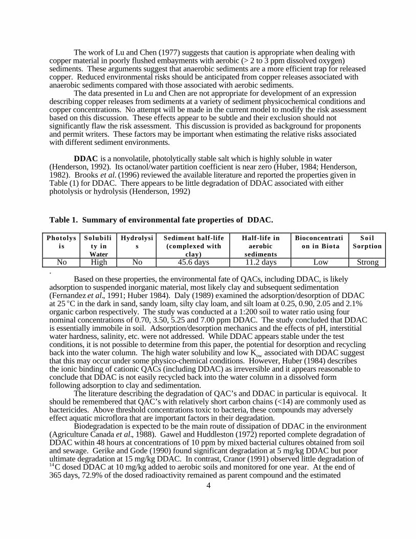
DDAC is a nonvolatile, photolytically stable salt which is highly soluble in water(Henderson, 1992). Its octanol/water partition coefficient is near zero (Huber, 1984; Henderson,1982). Brooks et al. (1996) reviewed the available literature and reported the properties given inTable (1) for DDAC. There appears to be little degradation of DDAC associated with eitherphotolysis or hydrolysis (Henderson, 1992)

Table 1. Summary of environmental fate properties of DDAC.

Photolysi s

Solubi l ity inWater

Hydrolysis

Sediment half-life(complexed with

clay)

Half-life inaerobic

sediments

Bioconcentration in Biota

So i lSorption

No High No 45.6 days 11.2 days Low Strong.

Based on these properties, the environmental fate of QACs, including DDAC, is likelyadsorption to suspended inorganic material, most likely clay and subsequent sedimentation(Fernandez et al., 1991; Huber 1984). Daly (1989) examined the adsorption/desorption of DDACat 25 oC in the dark in sand, sandy loam, silty clay loam, and silt loam at 0.25, 0.90, 2.05 and 2.1%organic carbon respectively. The study was conducted at a 1:200 soil to water ratio using fournominal concentrations of 0.70, 3.50, 5.25 and 7.00 ppm DDAC. The study concluded that DDACis essentially immobile in soil. Adsorption/desorption mechanics and the effects of pH, interstitialwater hardness, salinity, etc. were not addressed. While DDAC appears stable under the testconditions, it is not possible to determine from this paper, the potential for desorption and recyclingback into the water column. The high water solubility and low Kow associated with DDAC suggestthat this may occur under some physico-chemical conditions. However, Huber (1984) describesthe ionic binding of cationic QACs (including DDAC) as irreversible and it appears reasonable toconclude that DDAC is not easily recycled back into the water column in a dissolved formfollowing adsorption to clay and sedimentation.

The literature describing the degradation of QAC’s and DDAC in particular is equivocal. Itshould be remembered that QAC’s with relatively short carbon chains (<14) are commonly used asbactericides. Above threshold concentrations toxic to bacteria, these compounds may adverselyeffect aquatic microflora that are important factors in their degradation.

Biodegradation is expected to be the main route of dissipation of DDAC in the environment(Agriculture Canada et al., 1988). Gawel and Huddleston (1972) reported complete degradation ofDDAC within 48 hours at concentrations of 10 ppm by mixed bacterial cultures obtained from soiland sewage. Gerike and Gode (1990) found significant degradation at 5 mg/kg DDAC but poorultimate degradation at 15 mg/kg DDAC. In contrast, Cranor (1991) observed little degradation of14C dosed DDAC at 10 mg/kg added to aerobic soils and monitored for one year. At the end of365 days, 72.9% of the dosed radioactivity remained as parent compound and the estimated

5

anaerobic half-life of 1,048 days. Similar studies reported by Cranor (1991) estimated an aerobicaquatic half-life of 8,365 days and an anaerobic aquatic (microbially active water and sedimentdosed with 10 mg/kg DDAC) half-life of 6,218 days. The refractory nature of QACs in anaerobicconditions is further supported by Huber (1984).

New data, not reported in Brooks et al. (1996), was developed by the manufacturer usingnatural sediment obtained from three sites on the Saint Clair River in Canada (WildlifeInternational, 1996). This new study suggested that the half-life for DDAC in aerobic sediments is11.2 days. When DDAC was complexed with clay, the half-life increased to 45.6 days. Takenaltogether, this review suggests that the sedimented half-life of DDAC varies with the availability ofoxygen as well as the resident microbial community. No information was obtained as to whether ornot DDAC provides a suitable sole carbon source for some species of bacteria, or if it is catabolizedonly in the presence of other organic compounds. Some refractory compounds, like high molecularweight PAH, cannot be metabolized in the absence of more labile and complex carbon substrates. If this is true, then the half-life of DDAC would vary with the amount of sedimented TOC. However, the Wildlife International (1996) study used unamended, natural sediments, and theobserved half-life of between 11.2 and 45.6 days is likely more appropriate.

DDAC’s strong affinity for soils suggests that losses from ACQ-B preserved wood willadsorb to clay particles and be sedimented. Based on this discussion, it appears that DDAC isstable in sediments at concentrations exceeding (10 ppm), but is degraded with a half-life of 1.1 to45.6 days at lower concentrations. Additionally, it appears that DDAC degradation is dependent onoxygen tension in sediments and longer half-lives can be expected in anaerobic conditions or wheremicroflora are compromised.

Bioaccumulation of Copper and DDAC In Aquatic Environments.

Copper is an essential micronutrient for plants and animals. Its uptake and metabolism is anormal biological process. DDAC is an anthropogenic compound. This chapter discusses thepotential for the bioaccumulation of copper and DDAC by aquatic plants and animals.

Copper bioconcentration. The National Academy of Sciences (1971) provides copperbioconcentration factors for numerous taxa. These values range from 100x for benthic algae to30,000x for phytoplankton. Marine mollusks concentrate copper by a factor of 5,000 in muscleand soft parts. Anderson (1977) reported metal bioconcentration factors in six species offreshwater clams from the Fox River in Illinois and Wisconsin. He found that soft tissuescontained levels of copper equivalent to those found in sediments, which were significantly higherthan water column levels. Anderson (1977) reported water column concentrations of copper at0.001 – 0.006 µg/L or one to six parts per trillion. This appears to be low by a factor of 1000 andthese data appear suspect. Assuming that these reported water column concentrations are in error bya factor of 1,000, a comparison of the mean copper soft tissue burden (12.24 µg/g dry tissueweight) with the mean water column copper concentration (0.0035 mg/L) implies a BCF of 3,497. This value is consistent with the NAS (1971) copper bioconcentration factor for bivalve mollusks. Hendriks (1995) observed that dry weight corrected concentrations of copper in freshwater plantsand invertebrates from the Rhine Delta were 0.2 to 0.3 times the concentrations observed insuspended sediments – suggesting that copper adsorbed to suspended sediments is not readilybioconcentrated.

Marquenie and Simmers (1987) examined metal and polycyclic aromatic hydrocarbonlevels in sediments and earthworms (Eisenia foetida) at an artificial wetland site created on aconfined dredged material disposal facility that became a prolific wildlife habitat. At the six sitesreported, they found an average copper concentration of 192.5 + 107.6 µg Cu/g (dry weight) insoils. At the end of ca. 49 days, Eisenia foetida contained an average of 36.3 + 14.9 µg Cu/g (ash-free tissue weight) suggesting that much of the sedimented copper was not biologically available(BCF = 0.19). Control earthworms, collected outside the dredge disposal site, where soil copper

6

levels averaged 16.5 µg/g, contained an average of 10.1 µg Cu/g giving a BCF of 0.61 (three timeshigher). It is possible that 49 days was an insufficient period of time for annelid tissue to come intoequilibrium with the high environmental levels of copper. Alternately, it is also possible thatEisenia foetida is able to regulate copper uptake.

Rai et al. (1995) examined metal uptake from pond water amended with 1.338 µM (84ppm) copper in eight species of submerged macrophytes. No acute effects were observed –although several of the plant species did not increase biomass. At the end of 15 days, the plants hadremoved significant quantities of metal from the pond water and the bioconcentration factors givenin Table (2) calculated.

Table 2. Metal concentration factors (dimensionless) for submerged aquatic plants. From Rai et al. (1995). Metal Plant Cu Cr Fe Mn Cd PbHydrodictyon reticulatum 2481 11394 37666 8712 6250 5000Spirodela polyrrhiza 36500 7920 3878 3107 5750 2521Chara carallina 1103 2081 3029 2030 2125 2133Ceratophyllum demersum 53333 15332 37809 21600 3333 8064Vallisneria spiralis 2009 1993 1344 333 2375 1777Bacopa moonieri 18750 2016 2041 2487 29000 366Alternanthera sessilis 1051 722 1156 6395 23000 555Hygrorrhiza aristata 211 652 1138 1955 4600 7174

Copper uptake from the water column varied considerably from the concentration factorsranging from 211 in H. aristata to 53,333 in C. demersum. This study demonstrates high, butvariable copper bioconcentration factors in most plant species and demonstrates the potential forplants to remove copper from stormwater in retention ponds or biofiltration swales. However, it isdifficult to extrapolate from this study to natural environments where elevated copper levels wouldlikely be less than 15 to 20 µg/L rather than 84,000 µg/L.

Copper biomagnification. Little information was reviewed on the biomagnification ofcopper by aquatic organisms. Van Eeden and Schoonbee (1993) examined copper levels insediments, fennel-leaved pondweed ant various organs of the red-knobbed coot associated with ametal contaminated wetland in South Africa. They found that the pondweed contained less thanhalf the copper levels found in the sediments. Copper levels in the various organs of the coot weresimilar to those in the pondweed – except that very little copper was transferred to eggs (shell orcontents) of this bird. For the purposes of this paper, it will be assumed that copper accumulationin aquatic organisms is primarily a function of metal concentration in the ambient water. Whilemany organisms may bioconcentrate copper, the available information suggests that copper is notbiomagnified through food webs. The two processes (bioconcentration and biomagnification) arenot necessarily directly related. Many materials are bioconcentrated, particularly by bivalves. However, many of those bioconcentrated substances are not biomagnified because they are eitherrapidly excreted or metabolized.

DDAC bioconcentration. Henderson (1992) and Huber (1984) conclude that DDAC (orother QACs) are not significantly bioconcentrated. Huber (1984) cites several studies indicatingbioconcentration factors (BCFs) ranging from 5 to 32 for related QACs. Henderson (1992)reviewed this issue and reported a whole body bioconcentration factor of 81 for DDAC in thebluegill sunfish (Lepomis macrochirus).

Henderson (1992) assessed the pharmacokinetics of DDAC and concluded that becauseDDAC is highly ionic it is not expected to adsorb well across the gastrointestinal epithelium. Theresults of excretion studies in rats support this conclusion. Following oral dosing with 14C-DDAC,

7

89 to 99 percent of the radioactivity was found in the feces and less than 2.5% in the urine. Thisfinding was considered consistent with the predicted low absorption of DDAC. Absorbed DDACwas metabolized. The metabolic process was found to involve oxidation of the decyl side chain to avariety of oxidative products. Evidence seemed to favor initial hydroxylation of the carbon next tothe terminal carbon, followed by formation of a hydroxyketone. The four major metabolites foundin their study were more polar and presumed to be less toxic than the parent compound, althoughthe specific chemical structures were not determined.

Depuration experiments reported by Henderson (1992) indicated that 67% of the DDACaccumulated in whole fish tissues was depurated within 14 days. The available literature suggeststhat QACs, including DDAC do not significantly bioconcentrate in aquatic organisms.

DDAC biomagnification. No direct evidence examining this question was reviewed. However, based on the low observed bioconcentration factors, rapid depuration and observedmetabolism, biomagnification through the food chain is very unlikely and will not be considered anissue in this risk assessment.

Summary for the potential of Copper and DDAC to bioaccumulate. Copper isbioconcentrated at moderately high levels from the water column. It is not significantlybioconcentrated from sediments. No evidence of copper biomagnification was obtained. Theavailable evidence suggests that DDAC does not bioconcentrate in aquatic organisms and thepharmokinetics of DDAC suggests that it does not significantly biomagnify through food-webs.

Toxicity of Copper and DDAC to Aquatic Fauna and Flora. In order to assess the potentialimpacts of ACQ-B treated wood used in aquatic environments, it is necessary to determine theminimum levels of DDAC and copper causing acute or chronic stress in fauna and flora.

Copper toxicity in aquatic environments. Copper is an essential element for mostliving organisms. It is added at a concentration of 2.5 ppb in Guillard's Medium F/2 to sea waterfor the optimum culture of marine algae (Strathman, 1987). At concentrations slightly above thoserequired as a micronutrient, copper can be highly toxic; especially to the larval stages of marineinvertebrates. A single copper fitting in a seawater system may destroy most invertebrate embryosbeing cultured in the laboratory.

Copper in freshwater. EPA's (1984) Ambient Water Quality Criteria reports thatcopper toxicity in aquatic environments is related to the concentration of cupric (Cu2+) ions andperhaps copper hydroxides (CuOHn). The cupric ion is highly reactive and forms various coppercomplexes and precipitates which are significantly less toxic than the cupric ion (Knezovich, et al.,1981). Harrison et al. (1987) reported that copper discharged from the San Onofre power plantcooling system was found mostly in bound forms under normal operating conditions. Their studyfound sufficient organic ligands available in ambient seawater to complex most of the copper, andthey expected little or no impact from the discharges. Likewise, Nuria et al. (1995) and Kerrison etal. (1988) have observed that copper in freshwater lakes is generally associated with particulateorganic and inorganic material rather than with dissolved organic matter (DOM). These authorsconclude that natural water significantly reduces copper toxicity to aquatic organisms whencompared with laboratory systems manipulated using synthetic chelators like EDTA.

Sundra (1987) has proposed a basic mechanism explaining the observed relationshipbetween free ion activities and the bioavailability of metals such as copper. He observed that thecomplexed species of copper are charged or polar and cannot pass directly across the lipid bilayerof the cell membrane. Thus, transport of copper across the membrane would require that it interactwith specific metal transport proteins in the membrane. Because the free ion activity is a measure ofthe potential reactivity of a metal, it reflects the ability of that metal to interact with these transportproteins. The many chemical forms of copper in aquatic environments are maintained in a dynamic

8

state of equilibrium that depends on salinity, temperature, pH, alkalinity, dissolved oxygen, sedimentcharacteristics and the presence of other inorganic and organic molecules.

Clements et al. (1988) spiked freshwater mesocosms with 12 to 20 µg Cu/L and 15 to 27µg Zn/L. They found significantly reduced numbers of taxa, numbers of individuals andabundance of most dominant taxa within four days. After ten days, control streams were dominatedby Ephemeroptera and tanytarsid chironomids, whereas treated streams were dominated byHydropsychidae and Orthocladiini. Responses of benthic communities to metals observed at theClinch River (Russel County, Virginia), a system impacted by copper and zinc were similar to thosein experimental streams. Copper levels on the Clinch River varied from not detectable at upstreamcontrols to 105 µg/L at the point of discharge. Ephemeroptera and Tanytarsini, which comprised48 to 46% of the macroinvertebrate community at upstream reference stations, were significantlyreduced at all effluent sites. In this natural system, impacted stations were dominated byHydropsychidae and Orthocladiini. Interestingly, significant decreases in the number of all taxaand the abundance of individual species was observed at station (6), where 9 + 7 (one standarddeviation) µg/L Cu was observed. They found that Tricoptera and Orthoclad chironomids weretolerant of high levels of copper. The hardness at these Clinch River (Virginia) stations averaged169 ppm (CaCO3) and the alkalinity averaged 148 µg/L. At this hardness, the EPA chronic criteriais 17.8 µg/L. However, it should be noted that this station was directly downstream from thedischarge stations that had much higher levels (47 to 105 µg/L). Copper levels this high wouldlikely have significant effects on the drift community. This is seen in a follow-up study (Clements,et al. 1992) in which data from 1986 through 1989 were examined upstream and downstream fromthe power plant following a decrease in the copper content of the plant’s effluent from 480 µg/L in1987 to 260 µg/L in 1989. Copper concentrations were reduced at downstream Station (8) from127 µg/L in 1987 to 52.2 µg/L in 1989. The number of taxa increased from ca. ten in 1987 to 20in 1989. Only small decreases in both the number of taxa and the number of individuals persample were observed in 1989 suggesting only minor effects at the observed copper concentrationof 52.2 µg/L.

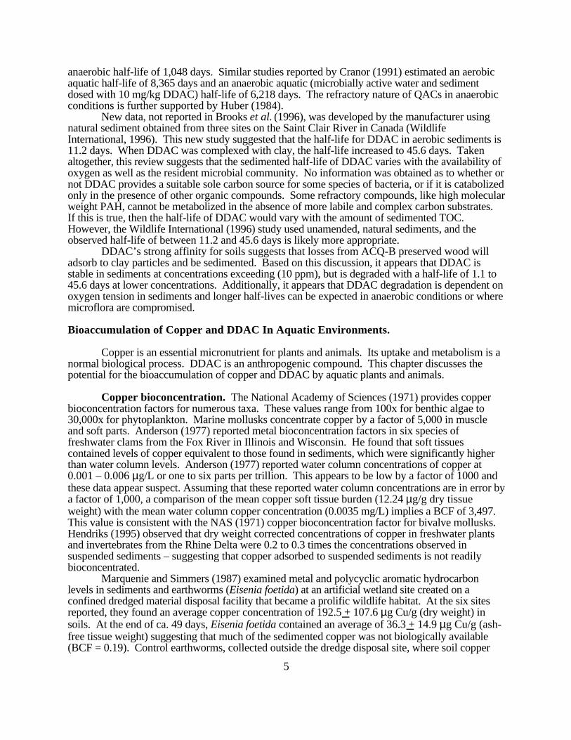
Gower et al. (1994) examined the relationship between invertebrate communities and avariety of metals in southwest England. Their work suggested that copper followed by aluminum,zinc, and cadmium, was the metal most responsible for influencing the observed changes in theinvertebrate community. Clements et al. (1982, 1992) found that Ephemeroptera and Tanytarsiniwere very intolerant of copper in the Clinch River whereas, Hydropsychidae and Orthocladidchironomids dominated impacted stations. The results of Gower et al. (1994) are summarized inTable (3). In this table, observed copper concentrations and hardness values are combined bydividing the observed copper concentration by the U.S. EPA chronic copper criteria at thedocumented level of hardness. These values should be interpreted as the numeric factors by whichobserved copper exceeded the U.S. EPA chronic freshwater standard. Community information isdisplayed by sample for each taxonomic group. The number of individuals in each taxonomicgroup is followed by the mean number of species, per sample, in parentheses.

Table 3. Mean number of total macroinvertebrates per sample (M), mean percentagecontribution of selected major taxa to the total macroinvertebrate fauna (P), and numberof species (S) observed by Gower et al. (1994) as a function of water column levels ofcopper expressed as proportional increases in the U.S. EPA freshwater copper criteria atthe observed level of hardness.

Ratio of dissolved copper to the U.S. EPA chronic freshwatercriteriaTaxonomic group 2.0 x 5.3 x 31.6 x 244.7 x

(M) (S) (M) (S) (M) (S) (M) (S)Macroinvertebrates 4598 39 989 21.3 2219 12.2 2378 9.2

9

(P) (S) (P) (S) (P) (S) (P) (S)Tricladida (flatworm) 7.7 1.3 3.4 1.0 15.0 1.1 30.2 0.8Oligochaeta 16.2 4.8 6.8 2.4 20.9 1.3 0.7 0.3Ephemeroptera 17.4 3.1 38.1 2.0 16.7 0.6 0.0 0.0Plecoptera 19.3 4.9 8.5 2.3 7.2 1.3 1.1 0.3Coleoptera 4.0 2.4 0.6 0.8 0.7 0.4 0.6 0.6Trichoptera (cased) 4.8 3.0 12.4 1.8 0.1 0.2 0.1 0.1Trichoptera (caseless) 4.8 3.4 14.7 3.0 5.4 1.8 4.8 1.3Total EPT1 46.3 14.4 73.7 9.1 29.4 3.9 6.0 1.7Chironomidae 16.9 8.0 11.3 4.4 31.1 3.8 60.3 3.8 Orthocladiinae 9.1 4.7 4.8 1.8 18.4 2.1 54.5 2.41 EPT refers to the aggregate numbers of insects in the orders Ephemeroptera, Plecoptera andTrichoptera.

These data are presented in some detail because they clearly demonstrate the insensitivity ofat least one flatworm species (Tricladida) some caddis flies (Trichoptera) and chironomids,particularly Orthocladiinae at very high water column concentrations of copper (245 x EPAstandard). Oligochaetes, caseless caddis flies and stone flies (Plecoptera) are relatively insensitiveat copper concentrations up to 32 times the EPA standard but the population was essentiallyextirpated at the highest levels of 245 times the EPA standard. It is certainly possible that caselesscaddis flies and stone flies represent the drift community in this study and the period of exposure toelevated copper concentrations is unknown. This observation is supported by the reduced numbersof resident (cased) caddis flies observed in areas where the copper concentrations exceeded theEPA chronic copper standard by a factor of 5.3.

Interestingly, the Order Ephemeroptera, frequently described as very susceptible to copperintoxication, represented nearly 40% of the macroinvertebrate community at 5.3 x the EPA standardand at least one species was able to tolerate 31.6 x the EPA standard. In addition to describinggeneral trends in copper susceptibility, these data suggest that some species in the sensitive ordersEphemeroptera, Plecoptera and Trichoptera are able to tolerate very high levels of copper -suggesting that increasing information is provided by identification of infauna to the level of genusor species. On the other hand, it should be noted that total species richness (number of species)declines monotonically and is perhaps the best indicator of increasing copper toxicity in this study. While the numbers of Ephemeroptera, Plecoptera and Trichoptera do not following thismonotonically decreasing trend, if we consider these Orders in the aggregate, we find that speciesrichness is inversely correlated with copper concentrations.

Kiffney and Clements (1994) examined the effects of heavy metals on a macroinvertebrateassemblage from a Rocky Mountain stream in experimental microcosms and found significantreductions in a number of taxa at their “1x” treatment of 12 µg Cu/L. The author’s stated that thisvalue was approximately equal to the U.S. EPA freshwater chronic copper standard at the measuredhardness of 38.3 mg/kg (CaCO3). However, at that hardness, the EPA acute criteria isapproximately half the tested concentration (6.9 µg/L versus 12 µg/L) and the chronic EPA criteriais only 38% of the test concentration. The results of this study followed that of others reportedherein. Significant reductions were observed in the Order Ephemeroptera, particularly in the familyHeptageniidae. A large variation was observed in chironomid response to copper with significantreductions in the Tanytarsini and Tanypodinae and a small reduction in the Orthocladiinae andChironomini.

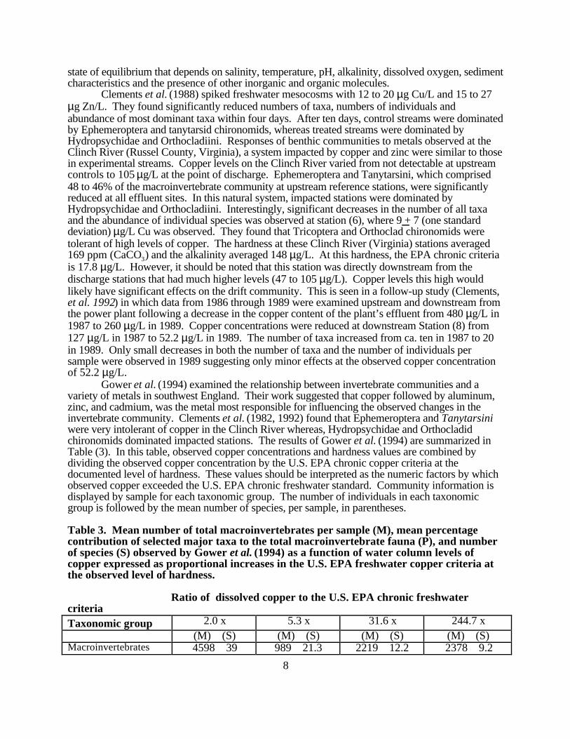
Rutherford and Mellow (1994) examined the effects of low pH and high dissolved metal(particularly copper) content on the fish and macroinvertebrates in beaver ponds located on anabandoned ore roast yard near Sudbury, Ontario, Canada. Table (4) summarizes the physico-chemical properties of the water at three of the sample stations. Hardness values were not providedin this study.

10

Table 4. Water chemistry at sample stations 1 (upstream), 3 (in roast pits) and 4(immediately downstream from roast pits) in the study of Rutherford and Mellow (1994).

Station pH Temp(oC) Dissolved Oxygen Copper ( g/L)1 (upstream) 6.7 22.2 8.0 183 (roast yard) 3.7 22.2 8.1 6004 (downstream) 6.2 23.3 7.6 45

Dissolved copper at all of the tested stations exceeded background levels by factors ofsix at Station One to 200 at Station Three. Other metals were elevated, but not to the very highlevels associated with copper and it appears reasonable to suggest that most of the effect seen in themacrobenthic community is associated with this metal.

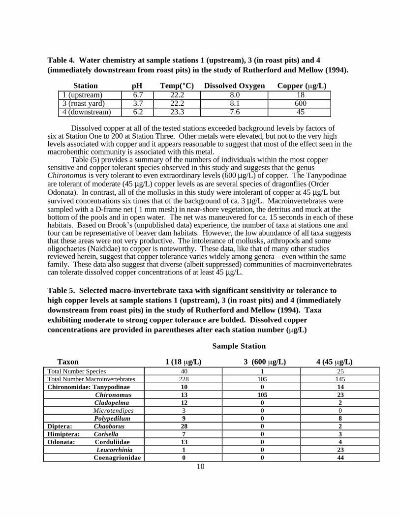
Table (5) provides a summary of the numbers of individuals within the most coppersensitive and copper tolerant species observed in this study and suggests that the genusChironomus is very tolerant to even extraordinary levels (600 µg/L) of copper. The Tanypodinaeare tolerant of moderate (45 µg/L) copper levels as are several species of dragonflies (OrderOdonata). In contrast, all of the mollusks in this study were intolerant of copper at 45 µg/L butsurvived concentrations six times that of the background of ca. 3 µg/L. Macroinvertebrates weresampled with a D-frame net ( 1 mm mesh) in near-shore vegetation, the detritus and muck at thebottom of the pools and in open water. The net was maneuvered for ca. 15 seconds in each of thesehabitats. Based on Brook’s (unpublished data) experience, the number of taxa at stations one andfour can be representative of beaver dam habitats. However, the low abundance of all taxa suggeststhat these areas were not very productive. The intolerance of mollusks, arthropods and someoligochaetes (Naididae) to copper is noteworthy. These data, like that of many other studiesreviewed herein, suggest that copper tolerance varies widely among genera – even within the samefamily. These data also suggest that diverse (albeit suppressed) communities of macroinvertebratescan tolerate dissolved copper concentrations of at least 45 µg/L.

Table 5. Selected macro-invertebrate taxa with significant sensitivity or tolerance tohigh copper levels at sample stations 1 (upstream), 3 (in roast pits) and 4 (immediatelydownstream from roast pits) in the study of Rutherford and Mellow (1994). Taxaexhibiting moderate to strong copper tolerance are bolded. Dissolved copperconcentrations are provided in parentheses after each station number ( g/L)

Sample Station

Taxon 1 (18 g/L) 3 (600 g/L) 4 (45 g/L)Total Number Species 40 1 25Total Number Macroinvertebrates 228 105 145Chironomidae: Tanypodinae 10 0 14 Chironomus 13 105 23 Cladopelma 12 0 2 Microtendipes 3 0 0 Polypedilum 9 0 8Diptera: Chaoborus 28 0 2Himiptera: Corisella 7 0 3Odonata: Corduliidae 13 0 4 Leucorrhinia 1 0 23 Coenagrionidae 0 0 44

11

Trichoptera: Oecetis 0 0 2 Banksiola 0 0 3Amphipoda: Hyallela azteca 3 0 0Naididae: 37 0 0Mollusca: Physa 8 0 0 Helisoma 29 0 0 Sphaerium 15 0 1Hirudinea: 5 0 0

In summary, these studies demonstrate trends in the relative sensitivity of freshwatermacroinvertebrates to copper intoxication. However, Gower et al. (1994) also points out that atleast some species within the sensitive EPT can tolerate very high levels of copper intoxication. Lastly, these data suggest that species richness for all fauna, or for the aggregated Orders EPT, isbetter correlated with the degree of copper intoxication than is an analysis at some lower levels oftaxonomic structure. Ammann et al. (1997) provided an excellent review of the idea of TaxonomicSufficiency for measures of impact in aquatic systems. They conclude that in at least one series ofstudies, identification and evaluation of infauna to the level of phylum was sufficient to documenteffects.

Copper in marine water. Roesijadi (1980) reported that copper is normally present atrelatively high levels in the tissues of marine animals (> 1,000 ppb). Roesijadi (1980), Harrison, etal. (1987) and Harrison and Lam (1985) review both the environmental detoxification of copperand the physiological detoxification of copper by Mytilus edulis, Protothaca staminea, Patellavulgata, Ostrea edulis and Littorina littorea. Copper detoxification and metabolic regulation wasassociated with copper binding by low and high molecular weight metallothionein-like proteins inthe digestive gland and the sequestering of copper in lysosomes. Costlow and Sanders (1987)used a metal-chelate buffer system to regulate the free ion concentration of copper in seawater. They exposed crab larvae to a range of free cupric-ion concentrations and monitored survival,duration of normal development and growth. The authors reported significant reductions in growthcorrelated with copper accumulation and concluded that when crab larvae are exposed to cupric ionconcentrations in seawater that are below ambient concentrations, they are able to regulate thebioconcentration of copper. At high concentrations of the cupric ion, copper bioconcentrationincreases in an unregulated manner and larval growth was inhibited.

Harrison et al. (1987) conducted copper bioassays on a number of aquatic invertebrate andvertebrate species. They found that Crassostrea gigas embryos were most sensitive (48-hour LC50=10 ppb) and larval herring the least sensitive. The range of 48-hour LC50 values for copper was10-2,000 ppb. Dinnel, et al. (1983) published the results of copper toxicity bioassays on variouslife stages of a number of marine organisms. They report a very low LC50 ( 1.9 ppb) for the spermof the red sea urchin (Strongylocentrotus franciscana). This value seems suspect because it fallswithin the range normally expected in unpolluted seawater. Reported values from the Dinnel, etal.(1983) study are presented in Table (6).

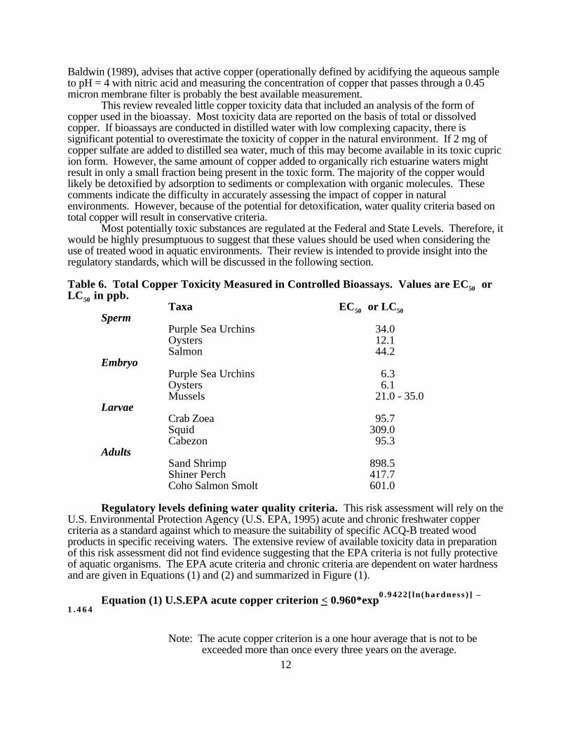
Gametes and embryos of marine organisms are most sensitive to copper. Based on theprevious discussion regarding the metabolic regulation of copper, it seems reasonable to suggestthat the susceptibility of embryos to even low copper concentrations is associated with their inabilityto regulate cellular exposure to the cupric ion. Copper levels maintained at levels low enough toprotect embryos are sufficient to insure that toxic effects are not imposed on larvae and adultorganisms. With the exception of the sperm of the red sea urchin, environmental levels less than 6ppb appear reasonable for the protection of aquatic life. In areas where red urchins spawn,additional restrictions should be considered.

Because of the variety of molecular structures containing copper in aquatic environments,and a lack of definitive information about their relative toxicity, no single analytical measurement isideal for expressing copper concentrations with respect to their potential toxicity to aquatic life.

12

Baldwin (1989), advises that active copper (operationally defined by acidifying the aqueous sampleto pH = 4 with nitric acid and measuring the concentration of copper that passes through a 0.45micron membrane filter is probably the best available measurement.

This review revealed little copper toxicity data that included an analysis of the form ofcopper used in the bioassay. Most toxicity data are reported on the basis of total or dissolvedcopper. If bioassays are conducted in distilled water with low complexing capacity, there issignificant potential to overestimate the toxicity of copper in the natural environment. If 2 mg ofcopper sulfate are added to distilled sea water, much of this may become available in its toxic cupricion form. However, the same amount of copper added to organically rich estuarine waters mightresult in only a small fraction being present in the toxic form. The majority of the copper wouldlikely be detoxified by adsorption to sediments or complexation with organic molecules. Thesecomments indicate the difficulty in accurately assessing the impact of copper in naturalenvironments. However, because of the potential for detoxification, water quality criteria based ontotal copper will result in conservative criteria.

Most potentially toxic substances are regulated at the Federal and State Levels. Therefore, itwould be highly presumptuous to suggest that these values should be used when considering theuse of treated wood in aquatic environments. Their review is intended to provide insight into theregulatory standards, which will be discussed in the following section.

Table 6. Total Copper Toxicity Measured in Controlled Bioassays. Values are EC50 orLC50 in ppb.

Taxa EC50 or LC50Sperm

Purple Sea Urchins 34.0Oysters 12.1Salmon 44.2

EmbryoPurple Sea Urchins 6.3Oysters 6.1Mussels 21.0 - 35.0

LarvaeCrab Zoea 95.7Squid 309.0Cabezon 95.3

AdultsSand Shrimp 898.5Shiner Perch 417.7Coho Salmon Smolt 601.0

Regulatory levels defining water quality criteria. This risk assessment will rely on theU.S. Environmental Protection Agency (U.S. EPA, 1995) acute and chronic freshwater coppercriteria as a standard against which to measure the suitability of specific ACQ-B treated woodproducts in specific receiving waters. The extensive review of available toxicity data in preparationof this risk assessment did not find evidence suggesting that the EPA criteria is not fully protectiveof aquatic organisms. The EPA acute criteria and chronic criteria are dependent on water hardnessand are given in Equations (1) and (2) and summarized in Figure (1).

Equation (1) U.S.EPA acute copper criterion < 0.960*exp0 .9422[ ln (hardness ) ] –

1 . 4 6 4

Note: The acute copper criterion is a one hour average that is not to be exceeded more than once every three years on the average.

13

Equation (2) U.S. EPA chronic copper criterion < 0.960*exp0 .8545[ ln (hardness ) ] –

1 . 4 6 5

Note: The chronic criterion is a four-day average concentration not to be exceeded more than once every three years on the average.

Figure 1. U.S. EPA chronic and acute copper criteria for freshwater. The copper standardis presented in g/L and hardness values in mg (CaCO3)/L.

Toxicity to aquatic organisms associated with sedimented copper. Cain et. al. (1992)compared copper concentrations in the insect orders Trichoptera and Plecoptera with concentrationsin mine waste contaminated sediments on the Clark Fork River in Montana. They observedsediment concentrations of 779 µg/kg in river reach 0 – 60; 408 µg/g in river reach 107 – 164 and129 µg/g in reach 192 – 381. These levels were significantly elevated above the 18 µg/g observedat unaffected reference sites. They found significant variability in uptake between varioustaxonomic and functional groups. Detritivores held higher levels of copper than either omnivoresor predators. This was especially true in the most contaminated reach (0 – 60 km). No appropriateanalysis of the community structure was presented.

Diks and Allen (1983) examined the bioavailability of different forms of copper associatedwith sediments. In their study, the distribution of copper was determined by assessing differentlevels of sedimented copper (0.0, 2.5, 5.0, 7.5 and 10.0 mg Cu/kg) in five geochemical fractions ofchemically extracted sediments, and in tubificid worms. They used five chemical extraction

0.0

10.0

20.0

30.0

40.0

50.0

60.0

70.0

Hardness in ppm (CaCO3)

Co

pp

er

cri

teri

on

in

mic

rog

ram

s/l

ite

r Acute Value

Chronic value

Acute Value 4.6 8.9 13.0 17.0 21.0 24.9 28.8 32.7 36.5 40.3 44.1 47.9 51.7 55.4 59.1 62.8

Chronic value 3.5 6.3 8.9 11.4 13.7 16.1 18.3 20.5 22.7 24.8 26.9 29.0 31.1 33.1 35.1 37.1

25 50 75 100 125 150 175 200 225 250 275 300 325 350 375 400

14

protocols with a range of aggressiveness in liberating copper from the five geochemicalcompartments being considered. The least aggressive was 1.0 M MgCl2, pH 7, with extraction atroom temperature for one hour. This procedure was considered appropriate for extracting only theabsorbed/exchanged copper. The most aggressive procedure was 1.0 M NH2O2.HCl in 25%HOAc, with extraction at 96oC for six hours. This procedure was considered sufficient to extractall copper including moderately reducible forms incorporated into the crystalline structure of ironoxides.

Diks and Allen (1983) found that free ionic metals, as well as most metals ion exchangedonto fine-grained solids were biologically available. Less available forms included metals containedin solid organic materials or precipitated and coprecipitated metal oxide coatings. Metalsincorporated into crystalline structures were not biologically available. Regression analysis wasused to evaluate the effects of the extraction technique and metal levels in each of the geochemicalcompartments on copper uptake by the tubificid worms. They found that only the copper extractedfrom the manganese oxide/easily reducible phase was significantly correlated (α = 0.05) withcopper uptake. They suggested that the redox potential and pH in the gut of the worm was suchthat manganese oxide coatings were dissolved during digestion making the copper available foruptake. This study suggests that the 0.1 M NH2OH.HCl + 0.01 M HNO3, pH = 2 extraction,conducted at room temperature for 30 minutes (See Chao, 1972) is most appropriate fordetermining biologically available copper in sediments. This is important because in the foursediments tested at 10 mg Cu/L (Des Plaines, Calumet, Flatfoot and Wabash), the proportion ofcopper biologically available in the amended sediments averaged 72%. The remaining 28% wasfound in geochemical phases that appeared to not be biologically available. Even more striking wasthe distribution of copper in the natural (unamended) sediments. In these natural sediments, only35% of the total copper burden appeared to be biologically available while 65% was incorporated inbiologically unavailable geochemical phases.

The purpose of this discussion is to suggest that extraction techniques and the biologicalavailability of copper in sediments are important parameters to the determination of sedimentstandards against which to assess biological risks. For purposes of this assessment, a mildlyaggressive extraction technique such as that (Chao, 1972) is recommended. More aggressiveextraction techniques used for assessing background copper may result in assuming a higher thanappropriate existing level of biologically available copper, leading to an overly conservativeassessment, whereas less aggressive extraction techniques may result in assessments that areinsufficiently protective of biological resources.

Flemming and Trevors (1988) dosed a calcareous, southern Ontario stream sediment withup to 10,000 µg Cu(II)sulfate/g dry sediment and examined its uptake of copper and microbialresponse. They found that sediment uptake of copper was nearly 100% to 2,800 µg Cu/g. Athigher levels of copper, the sediment uptake capacity was diminished and at 10,000 µg Cu/gsediment, only ca. 60% of the copper was removed from the water column. Aerobic heterotrophicbacteria were unaffected at the end of two months in sediments amended with as much as 1,000 µgCu/g sediment. Bacterial colony counts actually increased at higher copper levels. The authorsattributed this to the development of a population of copper tolerant microorganisms. The bacterialcommunity from the high copper amended sediments displayed a 500-fold increase in coppertolerance over bacteria from control sediments when plated on nutrient agar amended with excesscopper. The authors suggested that 87.5% of the copper added in these studies was transformedfrom the toxic Cu+ form to carbonate complexes (87.5%); 12% was complexed with dissolvedorganic matter and that only 0.5% was available as potentially toxic copper hydroxide complexes oras the toxic Cu+2 free ion. The point in this discussion is that calcareous sediments cansignificantly reduce the toxicity of very high concentrations of cupric ions. At least that statementappears true for the microbial community.

Munkittrick et al. (1989) examined the response of aquatic invertebrates to a gradient ofcopper and zinc contamination associated with mining activities along the Manitouwadge chain oflakes in northern Ontario. Their data are summarized in Table (7). The 22.7 + 6.4 mg Cu/kg

15

sediment at Station (3) on unaffected Loken Lake (LOK) is not significantly different from the levelof 25 + 8 mg Cu/kg sediment at Station (3) on impacted Manitouwadge Lake (MAN). However,the water column copper concentration at unaffected LOK was only 1.7 µg/L compared with 9.8µg/L at significantly impacted MAN. Station (1) at Lake Manitouwadge (MAN) has the highestlevel of sediment copper (160 mg/kg) of the three stations in that lake. This station also has thehighest abundance (12,838 invertebrates/m2), the highest diversity (21 species/sample) and thehighest number of typically sensitive cladocerans when compared with the other two stations in thislake, each of which has lower levels of sedimented copper. Munkittrick et al. (1989) also presenteddetailed enumeration of the Chironomid species in each lake. Interestingly, for nearly all genera ofChironomids, the sample station with the highest levels of sedimented copper in lake MAN alsohave the highest number of Chironomid species. It is interesting to note that the copper intolerantchironomid genera Polypedilium, Cladotanytarsus and Tanytarsus, are abundant in the control lakeLOK and present only at Station (3) (the station with the highest sediment concentration of copper)in affected Manitouwadge Lake.

In contrast, under conditions of the reported low water column copper concentrations inLoken Lake, there is an apparent decrease in the number of sensitive amphipods, gastropods andoligochaetes at the station with the highest sedimented copper concentration (Station 3 @ 22.7 mgCu/kg sediment). This pattern was also observed in the more detailed chironomid taxonomy whereStation (3) typically held as many or more chironomids of all genera than did the other stations withlower levels of sedimented copper. I say generally true because Polypedilium simulans wasobserved in much lower abundance at Station (3) than at the other reference stations.

These observations suggest that the primary invertebrate response in these lakes wasassociated with elevated water column concentrations of copper and not to the sedimented levelswhich spanned a large range of values. This is likely because the sedimented copper is notbiologically available. The point is that the elevated water column concentrations of copper inaffected Lake Manitouwadge appear to be masking any effect associated with sedimented copper upto the observed level of 160 µg Cu/kg dry sediment weight.

Miller et al. (1992) further examined the Manitouwadge chain of lakes. They reportedaverage water column concentrations of 15 µg/L in Manitouwadge Lake at a hardness of 110ppm CaCO3. This exceeds the U.S. EPA copper criterion for freshwater (12.31). Sedimentedcopper in Manitouwadge Lake averaged 93 mg Cu/kg sediment. No significant difference wasobserved in the standard length, weight, age or condition factor of white suckers betweenManitouwadge Lake and Loken Lake. Copper levels in invertebrates (tissue levels) weresignificantly correlated (Spearman’s correlation at p< 0.01) with water column concentrations ofcopper, but not with sediment copper concentrations over a wide range of values.

Table 7. Summary of copper concentrations in the water column and sediments ofreference Loken Lake (LOK) and impacted Manitouwadge Lake (MAN). Significantmacro-invertebrate data are included to indicated faunal response. All values are inmg/kg. Data are taken from Munkittrick et al. (1991).

End Point LOK (1) LOK (2) LOK (3) MAN (1) MAN (2) MAN (3)Sediment Copper 7.5 4.0 22.7 160.0 123.0 25.0Water Copper 0.0032 0.0013 0.0017 0.0098 0.0095 0.0098Cladocera 1484 1746 5326 437 175 87Copepoda 172023 1383 4366 1834 1048 262Chironomids (Total) 11701 20585 13598 9868 5502 4017 Procladius 1659 1878 4803 1834 2358 873 Cryptotendipes 262 74 0 1048 0 87

16

Pagastiella 175 144 87 4629 3057 1310 Polypedilium 5852 4544 1572 0 0 0 Cladotanytarsus 873 6113 1921 1397 0 175 Tanytarsus 1659 5458 2620 262 0 175Total Abundance 47069 36083 25737 12838 8035 5240Diversity 36 35 28 21 8 17

Kraft and Sypniewski (1981) examined the effects of high sedimented copper on themacroinvertebrate community of the Keweenaw Waterway. They found high concentrations ofcopper (<589> mg Cu/kg dry sediment) in areas where the sediment consisted of ca. 66% silt andclay and much lower copper levels (<33> mg Cu/kg dry sediment) in areas where the silt-claycontent averaged 27% if the sediment grain size matrix. They observed significant differences incommunity structure with Hexagenia, Tanytarsus, Peloscolex, Sphaerium (mollusk) andPontoporeia (arthropod) virtually excluded from the area with the high copper content. In contrastthe area with high sedimented copper held more individuals in the genera Chironomus, Atribelos,Limnodrilus, Ceratopogonidae and Dicrotendipes.

Moore et al. (1979) compared sediment concentrations of arsenic, mercury, copper, lead andzinc with infauna in a series of lakes downstream from the Con Mine in the Canadian subarctic. Ingeneral, all of the metals were significantly elevated in the upstream water column and sediments,complicating the analysis. Observed metal and infauna data is summarized in Table (8).

The sediments and water column in Meg Lake are significantly impaired by each of themetals investigated. The most common species was the bivalve, Pisidium casertanum, which isapparently very tolerant to metal intoxication. Seven chironomid and six mollusk species wereobserved in Keg Lake under the influence of very high metals content in sediments and the watercolumn. Cironomids represented up to a maximum of 60% by numbers in the benthos withProcladius culiciformis and Psectrocladius barbimanus dominating. Unlike Meg Lake, Pisidiumcasertanum was rare in Keg Lake with Physa jennessi, Valvata sincera and Lymnaea elodesdominating at various times of the year. Metal levels between Meg and Keg Lakes were similar andit must be assumed that other environmental parameters were responsible for the shift in themollusk community. Metal levels dropped significantly in Peg Lake where a total of 14 specieswere found (8 chironomids, 5 mollusks and one amphipod). Infaunal abundance increasedsignificantly to 5,500/m2 in Peg Lake – likely in response to the reduced metal concentrations.Further reductions were observed in Great Slave Lake. Sedimented copper levels were only ca.15% and arsenic was only 3%of the maximum found in Keg Lake. Baseline infauna and metalswere not evaluated at a remote (control) site in Great Slave and it is not possible to determinewhether or not conditions reported in this paper are representative of background. However, 44species were observed in these samples with a mean abundance of ca. 3100 infauna/m2. Considering the high latitude at which this study was conducted, these numbers are similar to thoseobserved at un-impacted reference areas by the author (Brooks, unpublished data). These datasuggest that reasonably abundant and diverse infauna can be associated with copper levels as highas 82 µg Cu/g (dry sediment).

Table 8. Comparison of metal levels and infauna at four lakes downstream from the ConMine in the Canadian subarctic. All metal concentrations are in mg/kg (dry sedimentweight).

Endpoint Meg Lake Keg Lake Peg Lake Great Slave Lake Sediment Water Sediment Water Sediment Water Sediment

WaterArsenic 539 2.000 349 1.900 76 0.700 12 0.020Mercury 132 47 80 53

17

Copper 477 0.200 544 0.050 106 <0.020 82 <0.020Lead 11 0.100 8 0.100 8 <0.020 14 0.008Total Number Species 9 13 14 44Number of Insect Species 5 7 8 25Number Mollusk Species 4 6 5 10Total Infaunal Abundance 800 1300 5500 3100

Puckett et al. (1993) have shown that metals, including copper, are associated with the silt-clay fraction of sediments and that wetlands appear to be important repositories for metals adsorbedto these fine grained sediments. This finding supports the conclusion that copper adsorbs to siltand clay rather than the more coarse fractions of the sediment.

Rehfeldt and Sochtig (1996) observed high metal tolerance in Baetis rhodani. The larvae ofthis species are scrapers, picking up diatoms from the surface of stones. Depending upon thedevelopmental stage and the availability of food, B. rhodani can also feed on detritus. It is apolyvoltine species, occurring in different larval stages in rivers at all times of the year. Sedimentsin rivers studied by Rehfeldt and Sochtig (1996) contained between 30.7 and 2917.4 mg Cu/kgdry sediment. Baetis rhodani contained between 64.0 and 226.2 mg Cu/kg dry tissue weight. Copper content in the larvae were highly correlated with sediment copper concentrations (Spearmanrank correlation coefficient = 0.94, P < 0.01). Table (9) describes the sediment bioconcentrationfactor for this species. The data are from Rehfeldt and Sochtig (1996)

Table 9. Heavy metal contents of sediments and of larvae of Baetis rhodani collected fromsix rivers in the German Federal Republic. Sediment Bioconcentration Factors arecalculated for each river. All values are in mg Cu/kg dry sediment.

River Cu in Sediment Cu in B. rhodani Bioconcentration FactorOker (Probsteib) 2917.4 169.2 0.06Oker (Schladen 1985) 438.8 226.2 0.52Ecker 30.7 64.0 2.08Grane 365.7 168.2 0.46Laute 155.5 126.5 0.81Tolle 90.7 110.2 1.21

Water in these rivers was described as “soft” with neutral pH (7.1 to 8.5). The sedimentswere dried, ground to a powder, sieved to a particle size of < 2 mm. Metals were extracted byboiling in 100 ml of nitrohydrochloric acid for an unspecified period of time. This ratheraggressive extractive technique may have liberated copper from other than biologically availablegeochemical partitions as previously discussed. This would help explain the wide variability insediment BCF (0.06 to 2.08) documented in Table (9) for a single species. Alternatively, there maybe some copper regulation occurring because the copper concentration in B. rhodani is fairlyconstant, varying only by a factor of 3.5, with the lowest tissue burdens associated with the lowestsediment burdens. It is also interesting to note that dissolved copper concentrations in the RiverOker were very high at 132.9 + 53 µu/L (mean and 95% confidence interval) further suggestingthat B. rhodani can regulate copper uptake.

Significant differences were observed in the macrobenthic communities associated withpolluted and unpolluted rivers by Rehfeldt and Sochtig (1996). They found that gammaridamphipods were particularly intolerant of copper and that mayflies of the genus Baetus were highlytolerant to copper. Other species in the EPT group were found in both polluted and unpollutedstreams but at generally reduced numbers in polluted areas. Chironomids were found in reducednumbers in polluted streams. This suggests that tolerant chironomid species are probably notpresent in these watersheds.

18

Cairns et al. (1984) spiked control sediments from the Tualatin River and Soap Creek Pondwith varying levels of copper to achieve sedimented copper levels varying between 59 mg/kg and10,600 mg/kg. Overlying water in these experiments was continually renewed until the sedimentsand water came into equilibrium. They then conducted sediment bioassays using sensitive speciesof arthropods (Chironomus tetans, Daphnia magna, Gammarus lacustris and Hyalella azteca. Asummary of the test conditions and results are provided in Table (10).

There was little or no difference between control survival and survival of any species incopper spiked sediments at concentrations 488 to 618 mg Cu/kg dry sediment in Soap Creek Pond. Nine of the ten Chironomus tetans survived for ten days in sediment copper concentrations of1080 mg/kg. Four survived at concentrations to 3,950 mg/kg. Control and treatment survival of D.magna was equal (9/10) at sediment concentrations to 400 mg Cu/kg dry sediment. Thisexperiment suggests that copper is not bioavailable in sediment rich in organic carbon and a highpercentage of fines (silt and clay). This study also suggests that copper levels less than perhaps600 mg/kg have little biological consequence in these “robust” sediments.

Table 10. Summary of sediment types, test conditions and results of copper spikedsediment bioassays reported by Cairns et al. (1984).

Sediment 10-day LC50

Sediment % TOC % Silt-clay C. Tetans D. magna1 G. lacustris H. azteca

Tualatin River 1.8 59.3 2296 937 - -Soap Creek Pond 3.0 84.8 857 681 964 1078

1All bioassays were based on a ten day exposure except that for Daphnia magna which is a 48-hr LC50 .

Toxicity summary for sedimented copper. The bioavailability of sedimented copperappears dependent on sediment physicochemical characteristics including the proportion fines (siltand clay), overlying and interstitial water pH, hardness and dissolved oxygen, and the presence ofsedimented organic carbon. Background levels of copper reviewed in the assessment varied asshown in Table (11).

Table 11. Background freshwater sediment copper levels reviewed in this assessment. All values are presented in mg Cu/g dry sediment.

Source Geographic Location ReportedBackground

Siipola (1991) Lower Columbia River 18.0 to 66.0Tetra Tech (1994) Lower Columbia River 19.3 to 49.9Munkittrick et al. (1989) Loken Lake, northern Ontario 22.7 + 6.4 (ie. < 35.2)Munkittrick et al. (1991) northern Ontario 4.0 to 23.0Cairns et al. (1984) Tualatin River, Oregon 59.0Cairns et al. (1984) Soap Creek Pond, University of Oregon 210.0Cain et al. (1992) Clark Fork River in Montana 18.0Moore et al. (1979) Great Slave Lake 82.0Schmidt (1978) “unpolluted sediments from nearshore areas” 2.0 to 78.0

These data suggest that sedimented copper concentrations in unpolluted reference areas canvary from 2.0 to at least 80 mg Cu/kg dry sediment. Diks and Allen (1983) suggest thatmoderately aggressive copper extraction protocols, such as that of Chao (1972) are appropriate for

19

determining the bioavailable copper in sediments. More aggressive protocols using hot acidextraction techniques over extended periods of time will overestimate the amount of bioavailablecopper by liberating copper from the lattice structure of other minerals.

Given that copper delivered to the sediments from the overlying water column and that watercolumn and sediment concentrations are generally positively correlated, it appears that it is thecopper concentration in the overlying water column that is most influential on aquatic fauna andflora. Copper does bioconcentrate and Cain et. al (1992) present data suggesting that infauna,particularly detritivores, can bioaccumulate copper from sediments, copper does not appear tobiomagnify through food webs.

This review suggests that aquatic invertebrates vary significantly in their response tosedimented copper. For instance of the seven genera of midges described in these studies, five aretolerant of sedimented copper to levels exceeding 100 mg Cu/kg dry sediment. Only the generaTanytarsus and Polypedilium appear intolerant at levels of 123 to 160 mg/kg. It should be notedthat the concentration of water in the study of Munkittrick et al. (1991) was 9.5 to 9.8 µg Cu/L. Water hardness was not provided in the paper and it is not possible to assess whether the responseof these species was to copper in the water or sediments. Based on this review, it appears that onlyTanytarsus, Polypedilium, Hexagenia, Sphaerium and Pontoporeia potentially intolerant ofsedimented copper. It was not possible from the papers presented to determine whether or not theirsusceptibility was to sedimented copper or copper carried in the water column. Confirmation of thesusceptibility of these taxa to sedimented copper would require sediment bioassays, such as thatperformed by Cairns et al. (1984). This review indicates that many species are very tolerant toexceptionally high levels of sedimented copper (Table 12). Many of these tolerance levels are muchhigher than the background values presented in Table (11).

Table 12. Summary of the tolerance of various freshwater taxa to sedimented copper.

Taxon Relative Tolerance Source Sediment CuConcentration

(mg Cu/kg dry sediment) Cladocera

Daphnia magna Tolerant 5 681 to 937 Chironomids

Chironomus Tolerant 2,5 589 to 2296Procladium culciformis Tolerant 3 477 to 544Psectrocladius barbimanus Tolerant 3 477 to 544Dicrotendipes Tolerant 2 589Pagastiella Tolerant 1 123 to 160Polypedilium Intolerant 1 123 to 160Tanytarsus Intolerant 1, 2 123 to 589

EphemeropteraHexagenia Intolerant 2 589Baetis rhodani Tolerant 4 < 2,917

DipteraCeratopogonidae Tolerant 2 589

Table (12) continued

Taxon Relative Tolerance Source Sediment CuConcentration

(mg Cu/kg dry sediment) Molluska

20

Sphaerium Intolerant 2 589Pisidium casertanum Tolerant 3 477 to 544Physa jennessi Tolerant 3 477 to 544Valvata sincera Tolerant 3 477 to 544Lymnaea elodes Tolerant 3 477 to 544

AmphipodaPontoporeia Intolerant 2 589Gammarus lacustric Tolerant 5 964Hyalella azteca Tolerant 5 1078

OligochaetaLimnodrilus Tolerant 2 589

1) Munkittrick et al. (1991)2) Kraft and Sypniewski (1981)3) Moore et al. (1979)4) Rehfeldt and Sochtig (1996)5) Cairns et al. (1984)

Regulatory standards for copper with respect to marine and freshwater sediments. Washington State has developed Marine Sediment Quality Standards for metals in WAC 173-204-320. These standards are based on Apparent Effects Thresholds (AETs). Different jurisdictionsmay develop more, or less, stringent standards depending on a number of factors. For purposes ofthis risk assessment, the Washington State standard of 390 mg Cu/kg dry sediment weight will beused as a benchmark against which to judge the environmental acceptability of sedimentaccumulated copper in marine sediments.

Standards for freshwater sediments were not available from any jurisdiction. Jones et al.(1997) have summarized available toxicological benchmarks for screening contaminants of potentialconcern for effects on sediment-associated biota. The U.S. Department of Energy accomplishedthis work in an effort to identify benchmark levels of contaminants that warrant further assessment,or that are at a level that requires no further attention at hazardous waste sites. It should beemphasized that these benchmarks were not developed or intended as sediment quality criteria forsurface waters. The authors note that, “Sediment benchmarks must not be used as the solemeasure of sediment toxicity. Field studies and toxicity tests shall be the primary indicators oftoxicity of sediments; benchmarks may be used to determine which chemicals present in thesediment are most likely causing the toxicity.” The following approaches, and sedimentconcentrations for copper, were discussed:

Screening Level Concentration Approach (SLC). This approach estimates the highestconcentration of a particular contaminant in sediment that can be tolerated by ~95% of benthicinfauna. The SLC is derived from synoptic data on sediment chemical concentrations and benthicinvertebrate distributions. First, the species screening level concentration (SSLC) is calculated byplotting the frequency distribution of the contaminant concentrations over all sites (at least 10)where the species is present. The 90th percentile of this distribution is taken as the SSLC for thatspecies. Next, a large number of SSLCs are plotted as a frequency distribution to determine thecontaminant concentration above which 95% of the SSLCs occur. This final concentration is theSLC.

Dr. Connie Gaudat, Acting Head Soil and Sediment Section, Evaluation and InterpretationBranch, Guidelines Division of Environment Canada noted that the Ontario guidelines weredeveloped without reference to water or sediment pH, total organic carbon, sediment grain size orany other environmental parameter effecting the fate, transport, deposition and bioavailability of thecompounds under consideration (Gaudat, 1995; personal communication). In discussing copperfor instance, she stated that documentation of worst cases involving metals may have occurred withvery low pH values or coarse sediments. This may be especially true in Ontario, where the

21

guidelines were developed, because it lies on the continental shield characterized by low soilbuffering capacity and low pH. She noted that many pristine areas in Canada have backgroundlevels which exceed the Ontario guidelines. She stated that Environment Canada is developingsediment standards, but until those standards are developed, they (and the Ontario Ministry ofEnvironment) use site specific risk assessments to determine appropriate sediment quality criteria. She said that the site-specific standards are always greater than Ontario’s guidelines because theyseldom, if ever, encounter the worst case conditions associated with the guidelines. It should benoted that Jones et al. (1997) do not recommend the SLC method even for developing benchmarksagainst which to assess the potential biological effects of contaminants at hazardous waste sites.

Apparent Effects Threshold Approach. The AET approach uses data from matchedsediment chemistry and biological effects measures. Biological effects could be assessed by eitherbenthic community survey or sediment toxicity tests. An AET concentration is the sedimentconcentration of a selected chemical, above which statistically significant biological effects alwaysoccur. Jones et al. (1997) defended the use of estuarine benchmarks for evaluation of freshwatersites when freshwater benchmarks are not available. The Washington State Apparent EffectsThreshold for copper in marine environments is 390 µg Cu/g dry sediment.

National Oceanic and Atmospheric Administration (NOAA) Approach. NOAAannually collects and chemically analyzes sediment samples from sites located in coastal marine andestuarine environments throughout the United States. These data were used to evaluate three basicapproaches to the establishment of effects-based criteria: the equilibrium partitioning approach(applicable to nonionic organic compounds), the spiked-sediment toxicity test approach, and variousmethods of evaluating synoptically collected biological and chemical data in field surveys (Longand Morgan, 1991). Chemical concentrations observed or predicted by these methods to beassociated with biological effects were ranked, and the lower 10th percentile [Effects Range-Low(ER-L)] and median [Effects Range-Median (ER-M)] concentrations identified. The ER-L andER-M values were recalculated by Long et al. (1995) after omitting the few freshwater dataincluded in the Long and Morgan (1991) calculation and after adding additional, more recent data.

Jones et al. (1997) note that the NOAA values may be used to help identify sites with thepotential to cause adverse biological effects. They caution that these are not NOAA criteria orstandards and are not intended for use in regulatory decisions or any other similar applications. The NOAA ER-L for copper is 34 mg Cu/kg dry sediment and the ER-M is 270 mg Cu/kg drysediment.

Florida Department of Environmental Protection Approach. The Florida Departmentof Environmental Protection (FDEP) methodology is similar to the NOAA approach. The updatedand revised data set used by Long et al. (1995) was also used by MacDonald (1994) to calculateThreshold Effects Levels (TELs) and Probable Effects Levels (PELs). Unlike the ER-Ls and ER-Ms, the TELs and PELs also incorporate chemical concentrations observed or predicted to beassociated with no adverse biological effects (no-effects data). The TEL is the geometric mean ofthe 15th percentile in the effects data set and the 50th percentile in the no effects data set. The PEL isthe geometric mean of the 50th percentile in the effects data set and the 85th percentile in the noeffects data set. The TEL represents the upper limit of the range of sediment contaminantconcentrations dominated by no effects data. The PEL represents the lower limit of the range ofcontaminant concentrations that are usually or always associated with adverse biological effects(MacDonald, 1994). The FDEP TEL is 18.7 µg Cu/g dry sediment weight and the PEL is 108 µgCu/g dry sediment weight.

Recommended interim marine and freshwater sediment benchmarks for copperand DDAC. Jones et al. 1996 recommend that a suite of benchmarks be used in evaluating thepotential adverse effects associated with a chemical on a site specific basis. However elegant that

22

approach may be, the usual permitting of projects using treated wood, particularly personal usepiers and floats, ferry terminals, etc. does not warrant development of a project specific sedimentquality standard. Recognizing that both the U.S. EPA and Environment Canada have cautioned thatthe use of the following screening benchmarks are not appropriate as sediment quality standards. The values are provided in Table (13) as background.

Table 13. Summary of jurisdictional screening level benchmarks for screeninghazardous waste sites for contaminants of concern.

Jurisdiction Criteria in g/g

Washington State Marine Sediment Quality Criteria 390National Oceanographic and Atmospheric Administration ER-L = 34 ER-M 270 Florida Department of Environmental Protection TEL = 18.7 PEL = 110 Ontario Ministry of the Environment Screening Levels SLC Low = 16 SLC Severe = 110

The preceding discussion describing the bioavailability and toxicity of copper suggests thatsedimented total organic carbon, percent fines (silt and clay), pH, dissolved oxygen, water hardnessand alkalinity can all effect the bioavailability and toxicity of sedimented copper. The author wouldgreatly prefer to rely on well thought-out freshwater sediment quality standards. Unfortunately,those standards have not been developed. The only regulatory level is Washington State’sApparent Effects Threshold for copper in marine sediments at 390 µg/g. The previous reviewsuggests that this level is too high to protect freshwater benthic organisms.

Until appropriate freshwater sediment quality standards are developed, the benchmarksgiven in Table (14) are proposed for evaluating the benthic effects associated with copper lost frompreserved wood. These levels are consistent with the range at which threshold effects are reportedby Jones et al. (1997) and at which sediment effects were reported in the reviewed literature. Inaddition, they appear consistent with background levels of copper found in many parts of NorthAmerica and should avoid the curious penchant of some jurisdictions to invoke metal concentrationcriteria that are well below apparently unpolluted ambient levels. Loehr (1997) notes that severalstates have surface water quality arsenic standards in the range of 1.4 to 0.002 ppb. He notes thatthe average concentration of arsenic in five brands of bottled water was 4.2 ppb or 2,100 times thelowest of these standards. He further notes that surface water in Washington State contains 0.1 to1 ppb and that ocean water holds ca. 1.7 ppb. USDA (1980) reports that Washington well watercontains between 5.0 and 6.0 ppb and Oregon well water contains as much as 1,700 ppb arsenic. Mr. Loehr comments that it is illegal to dump any of the tested bottled drinking water into anysurface water.

Table 14. Recommended benchmarks for assessing the environmental risks associatedwith sedimented copper lost from pressure treated wood.

Sediment and Water Column Characteristics Acceptable levels of SedimentedCopper.

1. Coarse grained sediment (silt & clay <10%) 30 µg Cu/g dry sediment Total Organic Carbon < 0.5% Moderate to low pH (5.5 to 6.5) Low hardness and alkalinity (25 to 35 ppm CaCO3)

2. Intermediate sediments (silt & clay between 10% and 25%) 65 µg Cu/g dry sediment Total Organic Carbon between 0.5% and 1.5%

23

Neutral pH (6.5 to 7.5) Moderate hardness and alkalinity (35 to 100 ppm CaCO3)

3. Low energy, well buffered streams and lakes (fines > 25%) 100 µg Cu/g dry sediment Total Organic Carbon >1.25% Greater than neutral pH (pH > 7.5) High hardness and alkalinity (> 100 ppm CaCO3)

These values are higher than the NOEL and/or TELs described in Table (13). It should beemphasized that all of the values in Table (13) are based on worst cases and do not take intoconsideration environmental factors that mediate environmental toxicity. For instance, the Ontarioscreening criteria for sedimented copper (16 µg/L) is based on the worst cases in the Ontariodatabase, an area lying on the continental shield in which worst cases likely involve very low pH,low alkalinity and hardness and coarse (rocky) substrates. As previously discussed, EnvironmentCanada does not recognize these values as standards and cautions that background levels in otherparts of Canada consistently exceed this screening value with no evidence of toxic effects. Thebenchmarks provided in Table (14) are consistent with the range (28.5 – 96 µg Cu/g dry sediment)of threshold effects levels presented by Jones et al. (1997).

Some insight regarding the appropriateness of adopting the copper screening values inTable (14) as regulatory standards can be obtained by comparing similar data for the water columnwith the U.S. Environmental Protection Agency freshwater regulatory standard for copper, adoptedby many jurisdictions throughout the world. Suter and Tsao (1996) present conventionalbenchmarks for priority contaminants in freshwater. In Table (1) of their document they comparethe EPA chronic value for copper (12 µg/L at 100 mg/L hardness) with the lowest chronic values inthe literature (similar to the NOELs or TELs presented in Table (13) of this document forsedimented copper). The results are presented in Table (15).

Table 15. Summary of conventional benchmarks for copper in freshwater ( g/L). Thedata are from Suter and Tsao (1996). The Environmental Protection Agency NationalWater Quality Criteria for copper was computed at a hardness of 100 mg (CaCO3) /L.

Metal National Water Quality Lowest Chronic Values for:Criteria

Fish Daphnids Non Daphnid Aquatic Plants All Organicms Acute Chronic Invertebrates

Copper 18 12 3.8 0.23 6.066 1.0 0.23

All of the lowest chronic values are lower than the EPA chronic copper criteria at 100 mg/Lhardness. The literature clearly indicates that these lowest chronic values were likely obtained underconditions of low alkalinity, low total hardness, low levels of organic carbon (dissolved andparticulate), low levels of particulate inorganic carbon and low pH. These conditions areunrepresentative of most natural bodies of water; and therefore, adoption of the lowest chronicvalues as a standard would be unnecessarily restrictive. The lowest daphnid value (0.23 µg Cu/L) isless than ambient copper levels in most natural bodies of water.

It is unfortunate that regulatory standards have not been developed for sedimented copper infreshwater. Eventual development of appropriate standards by the Environmental ProtectionAgency will take into account the environmental factors that affect sedimented copper toxicity andwill provide reasonable estimates of sedimented copper that will not adversely affect biologicalresources.

24

Toxicity to aquatic fauna and flora associated with didecyldimethylammonium choride(DDAC). Brooks et al. (1996) conducted an extensive quality assurance review of thetoxicological database for DDAC and suggested that the LC50 values summarized in Table (16)represented the best estimates of true values. Brooks et al. (1996) reported that the toxicity offormulated products, using DDAC as the active ingredient, was lower than toxicity associated withthe technical grade.

Table 16. Summary of DDAC LC50 data for aquatic species from Brooks et al. (1996). Allvalues are in g active ingredient/L.

Species 96 hr. LC50

Sturgeon larvae (Acipenser transmontanus)1 0.001 to 0.010Sturgeon larvae (Acipenser transmontanus)5 0.415Zebra Fish1 0.172Fathead minnow (80% DDAC)1 0.195 (0.122 – 0.224)Bluegill sunfish (Lepomis macrochirus)4 0.320Bluegill sunfish (Lepomis macrochirus)4 0.295Bluegill sunfish (Lepomis macrochirus)4 0.270Rainbow trout (Oncorhynchus mykiss)1 0.466 + 0.1Rainbow trout (Oncorhynchus mykiss)4 1.24 (range = 0.52 to 2.81)Rainbow trout (Oncorhynchus mykiss)3 1.700 (1.4 –2.0)Coho salmon (Oncorhynchus kisutch)4 0.840 (range from 0.67 to 1.00)Catfish 1 0.590Chinook salmon (Oncorhynchus tshawytscha)1 0.705 + 0.015Chinook salmon (Oncorhynchus tshawytscha)4 0.360Guppies4 0.600Sheepshead minnow (80% DDAC)1 0.940 (0.770 – 1.200)Flounder1 2.050Catfish (96 hr LC50)4 1.300Daphnia magna1 0.052Daphnia magna (48 hr EC50)2 0.060 (0.051 – 0.072)

Mysid shrimp 0.069

Notes: 1 Farrel cited in Brooks et al. (1996) 4 Henderson (1992) 2 Handley et al. (1994c) 5 Schoenig (1998) 3 Handley et al. (1994b)

It should be noted that the sturgeon bioassay conducted by Farrell used yolk-sac and 30 to40 day old larvae. Anecdotal evidence provided by Dr. Gerald Schoenig (personal communication)suggested that Dr. Farrel’s sturgeon larvae were the survivors of two highly stressful eventsoccurring just prior to the DDAC bioassays. These stresses were created during shipping in whichhalf the larvae were lost and by the inadvertent introduction of lethal quantities of chlorine into theholding tank the day prior to the DDAC bioassays resulting in the loss of an additional 50% of thelarvae. Subsequent laboratory bioassays (AQUA-Science, 1997a) on 78 day old sturgeon larvaeindicate a 96-hr LC50 of 416 µg DDAC/L which is consistent with other fish bioassays. Testconditions were: temperature = 16 to 17 oC; dissolved oxygen = 5.4 to 9.8 mg/L; pH = 7.05 to7.79; hardness = 94 to 135 mg/L and alkalinity = 77 to 130 mg/L. This study also reported a 96-hrLC25 of 225 µg/L and a 96-hr NOEC of 100 µg/L.

A second larval sturgeon bioassay was conducted with the addition of ca. 1/16” of sedimentfrom the Fraser River in British Columbia to the bottom of the test chambers (AQUA-Science,1997b). This bioassay was conducted under similar physicochemical conditions but at reduced

25

alkalinity (57 to 89 mg/L) and hardness (43 to 110 mg/L). Higher toxicity thresholds weredetermined in the presence of sediment:

Endpoint µg DDAC/L

96-hr NOEC 2,40996-hr LOEC 8,03096-hr LC25 3,81496-hr LC50 5,220

For purposes of this report, the sturgeon bioassay data reported by Aqua-Science (1997a)will be used (96-hr LC50 = 416 µg DDAC/L). These data suggest that sturgeon larvae (Acipensertransmontanus) are not particularly sensitive to DDAC.

Only limited data were available describing the chronic effects of DDAC on aquatic species. Twenty-four hour exposures of rainbow trout to DDAC concentrations of 0.400 mg/L have beenshown to affect blood plasma glucose levels, plasma corticosteroid hormones and lactate levels andreduced swimming performance in rainbow trout was observed by Wood et al.,(in preparation, citedin Brooks et al. 1996) at 0.200 mg DDAC/L. Table (17) summarizes the available No ObservedEffects Levels for DDAC.

Table 17. Summary of no-observed effect levels (NOEL) measured for DDAC.

Species NOEL (mg/L)

Rainbow trout2 1.000Bluegill sunfish (Lepomis macrochirus) 0.100Coho salmon 0.590

Scenedesmus subspicatus (algae)1 1.000Daphnia magna3 0.032Daphnia magna4 0.074Mysid shrimp 0.052

Notes: 1 Handley et al. (1994a) 2 Handley et al. (1994b) 3 Handley et al. (1994c) 4 Henderson (1992)

Effects of Dissolved Organic Carbon. Wood leachate contains high levels of organicextractives in addition to preservative. Taylor et al. (1996) reported high biological oxygen demand(BOD) of 1,660 to > 2,600 mg/L in wood leachate. DDAC has the potential to bind to dissolvedorganic matter in water. In general, sorption of compounds to dissolved organic matter reducestheir bioavailability and thus their toxicity to aquatic organisms (Mills, 1993). SpringbornLaboratories (1994) indicated lower acute toxicity of DDAC to fathead minnows associated withincreasing levels of DOC. The results of this study are summarized in Table (18). These datasuggest that DDAC behaves like other organic molecules (PAH, etc.) in that toxicity is mediated bythe availability of organic material in the water column and in the sediments. Ultimately, theavailability of environmental levels of organic material (DOC, POC, sedimented TOC, etc.) shouldbe taken into account in developing either water quality or sediment standards for this material.

Table 18. The effect of DOC on toxicity of the antisapstain chemical, DDAC, to fatheadminnows in a 96 hr. static renewal acute toxicity test (from Brooks et al., 1996)

26

Amount of humic acid added toDDAC solution (mg/L)

96-hr LC50 (mg a.i./L) with95% confidence limits

NOEC (mg a.i./L)

0.0 0.19 (0.16 – 0.27) 0.09210.0 0.77 (0.65 – 1.0) 0.4020.0 1.2 (0.94 – 1.6) 0.94

DDAC toxicity to aquatic plants. Handley et al. (1994) reported a no-observed effectslevel of 1.0 mg/l with a 96 hr. EC50 of 3.0 mg/L for Scenedesmus subspicatus. The end pointsexamined in different tests were a 50% reduction in growth rate and a 50% reduction in biomass.

Henderson (1992) cited Walker and Evans (1978) in noting that QACs suppress growth inChlorella and duckweek (Spirodela oligorhiza) at concentrations above 3.0 to 5.0 mg/L. Induckweed, sublethal levels of QACs caused a yellowing or browning of the frond margins and theproduction of smaller sized fronds. In Chlorella, the size, shape, and internal organization of thecells were affected; death appeared to be due to disruption of chloroplast structures.

Carcinogenic, mutagenic and teratogenic effects. Henderson (1992) reviewed severalspecific studies describing each of these issues and found no evidence for adverse effects.Specifically, Henderson’s (1992) review suggests that DDAC does not have carcinogenic,mutagenic or teratogenic effects on mammals.

Recommended water column benchmarks for DDAC. Based on the availabletoxicological database described above, it appears that the geometric mean of the two values of theNOEL for Daphnia magna (0.049 mg DDAC/L) provide a conservative benchmark against whichto judge environmental risk. This value is considered conservative because non-linear regressionanalysis of the NOEL versus DOC data in Table (18) suggests an increase in the NOEL of exp0.116

x DOC (mg/L) as DOC increases. This very simple (and preliminary) analysis suggests that the NOELwould be 12% higher at 1.0 mg/L DOC and 42% higher at 3.0% DOC; both of which are realisticlevels. A summary of the DOC data and regression analysis is provided in Figure (2). Thephysicochemical interactions resulting in the observed decrease in toxicity are unknown. Based onthe very low (near zero) octanol-water partition coefficient, it would not appear that DDAC wouldreadily complex with DOC.

27

Scatterplot (DDACTOC.STA 10v*10c)

y=0.102*exp( 0.116*x)+eps

DOIC

NO

EL

0.0

0.2

0.4

0.6

0.8

1.0

-2 2 6 10 14 18 22

Figure 2. Effect of Dissolved Organic Carbon (DOC) on the No Observed Effect Level of DDAC to fathead minnows in a 96 hour static renewal acute toxicity test (data fromSpringborn Laboratories). DOC and NOEL data are in mg/L.

It was the conclusion of the Antisapstain Review Committee in British Columbia thatinsufficient evidence existed for lowering the stormwater discharge criteria from 700 µg DDAC/ to395 µg DDAC/L. It should be noted that applying a safety factor of ten to the current dischargelimit of 700 µg DDAC/L results in an allowable receiving water concentration of 70 µg DDAC/L,which is higher that the 49 g DDAC/L benchmark chosen for this assessment

Aquatic toxicity associated with sedimented DDAC. ABC Laboratories (1995) examined thetoxicity of DDAC incorporated into sediments to the midge (Chironomus tetans). Test chamberswere maintained in a temperature-controlled waterbath with temperatures ranging from 21 to 22 oC. Dissolved oxygen ranged from 3.3 to 8.1 mg/L throughout the test. Water pH ranged from 6.9 to8.3. Measured endpoints included survival and growth at the end of 14 days as well as survival andemergence success at the end of 28 days exposure. The 14-day and 28-day LC50 values werecalculated at >1,000 and 2085 mg/kg respectively. A 14-day EC50 value was calculated at 1,287 mgDDAC/kg based on total observed adverse effects (decreased size and mortality). The NOEC,based on larval weight and time to emergence was 530 mg DDAC/kg. The geometric meanmaximum acceptable toxicant concentration (MATC) calculated from the above data was 728mg/kg.

No empirical evidence describing the fate and transport of DDAC in open aquaticenvironments was available. The very high water solubility and low KOW of DDAC suggests that itwill likely bind ironically to finely divided inorganic particulate material, particularly clay, in thewater column. The strong sorption to soils reported in Brooks et al. (1996) suggests little

28

propensity to desorb and re-enter the water column form sediments. No information was availabledescribing the potential for infaunal detritivores to ingest DDAC sorbed to clay particles or for themovement of this material across the gut epithelia. However, Henderson (1992) observed poorabsorption of DDAC across the gut of fish, very low bioconcentration factors and a small potentialfor biomagnification through food chains. He also reported that fish rapidly catabolize and/orexcrete DDAC. Based on this evidence it appears unlikely that significant biological risks toeukaryotes will be associated with DDAC at sedimented values less than ca. 500 to 700 mgDDAC/kg. There is evidence that sediment concentrations above 10 mg DDAC/kg could effectmicrobial flora resulting in unknown changes in nutrient fluxes and decomposition of organicmatter in sediments.

Recommended sediment benchmark for DDAC. For purposes of this report, theassumption will be made that DDAC, dissolved in the water column, adsorbs to clay particles thatare deposited in sediments. Furthermore, this assessment concludes that risks associated withsedimented DDAC are acceptable at levels less than 10 ppm. It is acknowledged that thisassessment is based on inadequate information. A better understanding of the potential forbiological risk could be achieved with laboratory experiments designed to examine the transport ofDDAC from the water column to sediments and to examine the effects of sedimented DDAC oninfaunal communities of freshwater organisms. The data for larval sturgeon and midges discussedabove suggests that this benchmark of 10 mg DDAC/kg dry sediment is very conservative whenapplied to eukaryotes.

Summary statement regarding recommended benchmarks for dissolved and sedimentedcopper and DDAC for use in this risk assessment. Copper is an essential micronutrient foundat levels of one to ten µg/L in anthropogenically unaffected surface water. It is the cupric ion(Cu2+) and perhaps some species of copper hydroxides (CuOHn) that are toxic. The form ofcopper in surface water is dependent on pH, alkalinity, hardness and the availability of organic andinorganic binding sites (DOC, PIM, POM, etc.). The U.S. EPA has defined a freshwater copperstandard that is dependent on hardness. The review conducted in support of this risk assessmentdid not find instances in which this standard was under-protective of aquatic fauna or flora. TheEPA copper standard for marine water (3.11 µg/L) is independent of other environmentalparameters and the value was also not found to be under-protective. These EPA criteria are used asbenchmarks against which to assess the environmental suitability of 0.4 pcf, ACQ-B pressuretreated wood used in aquatic environments.

Freshwater sediment standards for copper or DDAC were not available. Interimbenchmarks for sedimented copper in freshwater were derived from Jones et al. (1997). TheWashington State AET based marine copper sediment standard of 390 µg/g is adopted as abenchmark for this assessment.

DDAC is an ionic carbon molecule that is highly soluble in water and which strongly bindsto clay. DDAC is toxic at low levels but does not appear to bioconcentrate or biomagnify. The No-Observed-Effect-Level (NOEL) for Daphnia magna (49 µg DDAC/L) is adopted as a benchmarkin this risk assessment.

It appears that DDAC is not bioavailable in sediments. However, it exhibits anti-microbialactivity at concentrations above 10 mg DDAC/kg dry sediment weight and this value has beenchosen as a benchmark.

These benchmarks are summarized in Table (19). In healthy sediments, bioturbation isexpected to homogenize the upper three to four centimeters of the sediment column. Consistentwith the Puget Sound Estuary Protocols (1986), samples taken to determine background levels ofcontaminants or to evaluate contaminant levels after construction of a project should include the toptwo centimeters of the sediment column.

29

Table 19. Water and sediment copper and DDAC benchmarks against which to assess theenvironmental suitability of ACQ-B preserved wood used in aquatic environments.

Freshwater copper benchmark: EPA chronic criterion < 0.960*exp0.8545[ln(hardness)] – 1.465

Freshwater DDAC benchmark: 0.049 mg DDAC/L

Freshwater sedimented copper benchmark:

Sediment and Water Column Characteristics Recommended Copper Benchmark

1. Coarse grained sediment (silt & clay <10%) 30 µg Cu/g dry sediment Total Organic Carbon < 0.5% Moderate to low pH (5.5 to 6.5) Low hardness and alkalinity (25 to 35 ppm CaCO3)

2. Intermediate sediments (silt & clay between 10% and 25%) 65 µg Cu/g dry sediment Total Organic Carbon between 0.5% and 1.5% Neutral pH (6.5 to 7.5)

Moderate hardness and alkalinity (35 to 100 ppm CaCO3)

3. Low energy, well buffered streams and lakes (fines > 25%) 100 µg Cu/g dry sediment Total Organic Carbon >1.25% Greater than neutral pH (pH > 7.5) High hardness and alkalinity (> 100 ppm CaCO3)

Saltwater copper benchmark: EPA saltwater criterion < 3.11 µg Cu/L (dissolved copper)

Saltwater DDAC benchmark: 0.049 mg DDAC/L

Saltwater sediment copper benchmark: Washington States Standard of 390 mg Cu/kg

Saltwater sediment DDAC benchmark: 10 mg DDAC/kg dry sedimentAnticipated Environmental Impacts Resulting From the use of ACQ-B Treated Wood InAquatic Environments. Depletion of preservatives from treated wood can occur by leaching ofwater-soluble components, physical loss (abrasion) or chemical and biological degradation. Instudies of preservative depletion from treated wood, it may be impossible to identify themechanisms of depletion. When biological or chemical degradation is present, the results from thistype investigation will over-estimate the environmental loading. Examination of the surroundingmedium (i.e. water or sediments) may fail to account for preservative depletion by biologicaldegradation.

Numerous studies have examined treated wood in the form of sawdust, shavings or smallcoupons. This is done to speed the leaching process. These studies are valuable for assessing therelative permanence of different wood preservatives and the relative propensity of each metal forleaching. However, their results cannot reasonably be extrapolated to predict leaching from fullsized commodities used in the environment. When such extrapolations are made, they will grosslyoverestimate the potential for environmental contamination. These laboratory studies cannot besubstituted for good field studies using full size commodities in natural environments.

30

Leaching of copper and DDAC from ACQ-B treated wood. The copper and DDACleaching data presented in this assessment was developed by Chemical Specialties Incorporated(Jin, 1997).

Materials and methods. Six southern yellow pine posts, averaging 17.2 cm indiameter were cut into five to 12 inch long sections. The cut ends were sealed and the sections kiln-dried to a moisture content of 20% or below prior to treating with ACQ-B to an average retention of0.43 pounds per square foot (pcf) in the treated zone (range = 0.40 to 0.46 pcf). A retention of0.40 pcf required by the American Wood Preservers Association (AWPA, 1996) for southernyellow pine in contact with fresh water. The treated sections were covered for three to five days andthen kiln-dried to a moisture content less than 20% prior to introduction into the leaching system.

Four replicates of these 0.4 pcf treated sections were leached at each of four pH values (5.0,6.5, 8.0 and 8.0 at a salinity of 30 parts per thousand (ppt)). Each acid rinsed leaching containercontained 10 to 12 liters of distilled water amended with HCL and/or NaCl to achieve the desiredtest conditions. In addition, an untreated control from the same pole was leached at each of the fourpH and salinity values. The average water volume to exposed wood surface area was 3.95 ml/cm2.

Copper was analyzed in the leachate using Inductively Coupled Plasma (ICP) on Days 0.5,1.5, 3.0, 5.5, 10.5, 21, 38.5, 54, 66 and 76.5. Copper loss rates (µg/cm2/day) for each time intervalwere computed from the known surface area of the pole and the volume and cumulative coppercontent in the leachate.

DDAC content in the leachate was determined using HPLC with a two-phase titrationmethod for those samples below the detection limit of the basic HPLC method on days 0.5, 1.5, 3.0,5.5, 10.5 and 21. DDAC content in the leachate at that time had apparently stopped increasing. DDAC does not readily degrade in the water column (Brooks et al., 1996) and therefore it wasconcluded that measurable losses of DDAC were not occurring after day 21 and no further DDACanalyses were accomplished. DDAC loss rates (µg/cm2/day) for each time interval were computedfrom the known surface area of the pole and the volume and cumulative DDAC content in theleachate.

Results. The copper and DDAC data provided by CSI were analyzed independently usingnonlinear, multifactor regression analysis followed by analysis of variance. Because this is the onlyimmersed leaching study for ACQ-B treated southern yellow pine, the analysis is discussed indetail in the following paragraphs.

actors affecting ACQ copper leaching rates. Dahlgren (1975) suggests that from thewood treaters’ point of view, the most important factors determining the leachability of water bornewood preservatives are the retention and type of preservative, the drying and storage conditions, andthe choice of wood species. Other important parameters are the ion-exchange fixation capacity ofcopper, the natural pH of the receiving water, and the chemical composition and anatomy of thewood. This risk assessment is specific for ACQ-B used to preserve southern yellow pine at aretention of 0.4 pcf. There are several other factors that cannot be controlled by the wood treater.

Fixation. The quaternary ammonium compound in ACQ fixes in wood throughion exchange with anionic active sites and through other adsorption mechanisms at higher quatconcentrations (Archer et al., 1992). Quat is fixed predominantly onto lignin, although interactionwith holocellulose also occurs. Copper is fixed in wood through ion exchange reactions betweencupriammonium ions and acidic functional groups such as carboxylic acid groups associated withlignin and hemicellulose. Copper complexes with cellulose through hydrogen bonding withhydroxyl or amine nitrogen groups, or through replacement of an ammonia group from thecupriammonium ion with the hydroxyl ion of cellulose. In addition, copper also forms insolublecopper carbonate salts resulting from the loss of ammonia during drying (Chen, 1994). It is

31

assumed that the preservative was fixed in the wood by the covered storage followed by kiln dryingreported by Jin (1997).

Time after installation in aquatic environments. Leaching is strongly time-dependent especially during the first three days following immersion. The scatterplot provided inFigure (3) clearly illustrates this. Note that there is significant variability in the Day (0.5) metal lossrates. This is in part due to short term differences associated with water pH (see Figures 4 and 10). However, the magnitude of the pH variability is not sufficient to account for the range of copperloss rates seen on Day 0.5 (18.4 to 61 µg/cm2/ on day 0.5). In can be hypothesized that some ofthe variability is associated with varying amounts of preservative remaining on the surface of thewood. Surface deposits of ACQ-B would not have binding sites available and therefore would notbe well fixed to the wood structure. Dissolution of this surface preservative could account for theinitially high losses, with the pronounced break at ca. 3.0 days, followed by relatively lower copperloss. The exponential fit is provided to illustrate the difficulty in describing this data using a singlenon-linear relationship. This section discusses the way in which various environmental variablesaffect copper loss rates from ACQ-B treated wood. Piecemeal regression will eventually be used tomodel copper losses from ACQ-B treated wood.

Scatterplot (ACQ.STA 10v*120c)

y=7.459*exp( -0.028*x)+eps

DAY

CU

LO

SS

-10

0

10

20

30

40

50

60

70

-10 10 30 50 70 90

Figure 3. Copper loss as a function of time ( g/cm2/day) from southern yellow pine poles,treated to 0.4 pcf with ACQ-B preservative and leached into 10 to 12 liters of distilledwater amended to a pH of 5.0, 6.5 or 8.0 and in saltwater (30 ppm) at pH 8.0. Data fromJin (1997).

Environmental pH effects. In general, the loss of copper from other waterbornepreservatives in dependent on pH effects. Brooks (1997a) provides an assessment of the effects ofpH on copper loss from ACZA treated wood and Brooks (1997c) discusses this same issue forCCA-C treated wood. Figure (4) provides a scatterplot describing copper loss (in µg/cm2/day)from southern yellow pine pressure treated with ACQ-B to a retention of 0.4 pcf and leached at pHvalues of 5.0, 6.5 and 8.0. There is an apparent decrease in variability with increasing pH. This

32

suggests either that either the surficial deposits described in the previous section are more easilydissolved at higher pH, or that small scale differences in wood characteristic create physicochemicalconditions leading to variability in copper loss as a function of pH. The first alternative appearsmore likely because the sections were cut from the same poles and were large enough to average outat least small scale differences in wood characteristics. As will be seen, differences in copper lossassociated with pH were significant at α = 0.05.

Salinity effects. Copper loss rates were determined at salinity’s of 0.0 and 30.0parts per thousand in this study. A scatterplot describing the results for pH = 8.0 is provided inFigure (5). At a retention of 0.4 pcf, salinity was not a significant parameter in determining copperloss and was not included in the regression analysis. It should be noted that AWPA (1996)requires a retention of 2.5 pcf ACQ-B for southern yellow pine immersed in saltwater andtherefore, this risk assessment is not intended for marine uses.

Scatterplot (ACQ.STA 10v*120c)

PHC

UL

OS

S

-10

0

10

20

30

40

50

60

70

4.5 5.0 5.5 6.0 6.5 7.0 7.5 8.0 8.5

Figure 4. Copper loss as a function of pH ( g/cm2/day) from southern yellow pine poles,treated to 0.4 pcf with ACQ-B preservative, and leached into 10 to 12 liters of fresh,distilled water amended to a pH of 5.0, 6.5 or 8.0 and in saltwater (30 ppm) at pH 8.0. Data from Jin (1997).

33

Scatterplot (ACQ.STA 10v*120c)

SALINITY

CU

LOS

S

0

10

20

30

40

-5 0 5 10 15 20 25 30 35

V2 = 8

Figure 5. Copper loss ( g/cm2/day) from southern yellow pine poles, treated to 0.4 pcfwith ACQ-B preservative and leached into either freshwater (salinity = 0.0) or seawater(salinity = 30 g/L). Data from Jin (1997)

Combined temporal and pH effects. The data provided by Jin (1997) wassubjected to non-linear regression analysis with of immersion and pH as independent factors. Theresulting relationship is defined in Equation (3) and described in Figure (6).

Equation (3). Square root (Copper loss ( g/cm2/day)) = 1.42 + 14.6 x exp(-0.58x day – 0.14 x pH)

The given regression explains 85% of the variation in the database and all of the coefficientsare highly significant (P < 0.0000). A square root transformation of the dependent variable wasnecessary in order to meet the underlying assumptions for regression analysis (normally distributedresiduals and homoscedasticity). This relationship is described in Figure (6).

34

Figure 6. Copper loss ( g/cm2/day) as a function of time and pH from southern yellowpine poles, treated to 0.4 pcf with ACQ-B preservative and leached into freshwater at pHvalues of 5.0, 6.5 and 8.0. Data from Jin (1997)

It is apparent in the data and in Figure (6) that the influence of pH is confined primarilyto the initial leaching period (first 5.5 days) and that pH effects are not apparent beyond 5.5days. This is substantiated by regression on a database in which day was restricted to >5.5 andwhere the probability that the coefficient on pH was equal to zero, increased to p = 0.258 whichis not significant.

Summary of environmental effects describing the loss of copper from ACQ-B preservative. At a retention of 0.4 pcf, salinity is not a significant factor affecting copper lossesfrom ACQ-B preserved wood. These results indicate that near-term copper loss is a function ofboth time and pH. At immersion times greater than 5.5 days, pH is no longer a significant factorand copper losses are only a function of time.

Environmental factors affecting the loss of DDAC from ACQ-B treated wood. Figure (7) describes DDAC losses in µg/cm2/day as a function of time at all pH and salinityvalues tested. Initial losses decline very quickly and are near zero within three days. The fittedexponential relationship is that which was eventually used to model DDAC losses from ACQ-Btreated wood at 0.4 pcf when used in freshwater.

3D Surface Plot (ACQ.STA 10v*120c)

Distance Weighted Least Squares

35

Figure 7. DDAC losses from 0.4 pcf ACQ-B treated southern yellow pine as a function oftime at pH = 5.0, 6.5 and 8.0 and at salinities of 0.0 and 30.00 ppt. Data from Jin (1997).

DDAC loss as a function of pH. DDAC losses were not a function of pH (P = 0.996)at the environmentally realistic values tested by Jin (1997) and was not included as a parameterin developing the final DDAC loss algorithm. Losses, expressed as a function of pH for allvalues of time and salinity are provided in Figure (8).

Model: V6 = A*exp(-B*V1)

y=(77.248556)*exp(-(1.533974)*x)

DAY

DD

AC

LO

SS

C:1

C:2

C:3

C:4

C:5

C:6

C:7C:8C:9

C:13

C:14C:15

C:16

C:17C:18

C:19C:20

C:21

C:25C:26

C:27

C:28

C:29

C:30C:31C:32C:33C:37

C:38

C:39

C:40

C:41C:42C:43C:44

C:45

C:49C:50C:51C:52C:53C:54C:55C:56C:57

C:61C:62C:63C:64C:65C:66C:67C:68C:69

-15

-5

5

15

25

35

45

55

5 10 15 20

36

Figure 8. DDAC losses from 0.4 pcf ACQ-B treated southern yellow pine as a function ofpH at values of 5.0, 6.5 and 8.0 for all times and salinities reported in Jin (1997).

Scatterplot (ACQ.STA 10v*120c)

PH

DD

AC

LO

SS

-15

-5

5

15

25

35

45

55

4.5 5.0 5.5 6.0 6.5 7.0 7.5 8.0 8.5

37

DDAC loss as a function of salinity. DDAC was negatively correlated withsalinity (decreasing DDAC loss with increasing salinity). However, the correlation was notsignificant and linear regression analysis (only two values for the independent variable) indicated anonsignificant coefficient (P = 0.12). Salinity was not included in the final algorithm describingDDAC loss from ACQ-B treated wood. The results provided in Jin (1997) are described in Figure(9).

Figure 9. DDAC losses from 0.4 pcf ACQ-B treated southern yellow pine as a function ofsalinity at a pH value of 8.0 for all times reported in Jin (1997).

Leaching of copper and DDAC from 0.4 pcf, ACQ-B treated southern yellow pineused in fresh water. Because of the apparent discontinuity in the copper loss data described inFigure (3), the copper loss algorithm was developed using piecemeal regression. The break was at4.5 days. Equation (4) defines the algorithm used in this risk assessment to describe copper lossesduring the first 4.5 days. This equation is valid for pH values between 5.0 and 8.0 and for timesbetween 0.5 and 4.5 days. This relationship will be used to compare maximum copperconcentrations in the water column within 2 cm of the treated wood on the first day of immersionwith the EPA chronic criteria (Equation (2) to assess the environmental suitability associated withACQ-B preservative use in a specific project.

Equation (4). Copper loss ( g/cm2/day) for days < 4.5 = 265.14 x exp(-0.924 x day – 0.239 x pH)

Copper losses at times greater than 4.5 days are described by the relationship given inEquation (5).

Equation (5). Copper loss ( g/cm2/day) for days > 4.5 = 4.25 x exp-0.0175 x day

Scatterplot (ACQ.STA 10v*120c)

SALINITY

DD

AC

LO

SS

-15

-5

5

15

25

35

45

55

-5 0 5 10 15 20 25 30 35

pH = 8.0

38

DDAC losses are predicted by the single algorithm provided in Equation (6).

Equation (6). DDAC loss ( g/cm2/day) = 77.24856 x exp-1.534 x day

Predicted copper and DDAC loss rates (µg/cm2/day) from 0.4 pcf ACQ-B treated southernyellow pine are summarized in Figure (10). These algorithms will be used as a basis for this riskassessment.

Figure 10. Summary of predicted copper and DDAC losses in g/cm2/day from 0.4 pcf,ACQ-B treated southern yellow pine in receiving water with a pH of 7.0.

Preservative loss from overhead structures. Rainfall, leaching studies appropriate forassessing copper and DDAC losses from overhead structures, decks, etc., were not available. However, the loss rates described in Figure (10) can be used to estimate risks until appropriate dataare available.

The leaching rates estimated by Equations (4) (5) and (6) provide a means of estimating thefinal environmental concentrations of copper and DDAC associated with the use of ACQ-B treatedwood products. Three Microsoft EXCEL based spreadsheet models are presented in thefollowing sections. The first describes anticipated levels of copper resulting from the use of ACQ-B treated piling installed in streams, rivers and lakes. The second predicts water column andsediment levels of copper and DDAC associated with large surface area wood structures such asbulkheads. The third is appropriate for assessing risks associated with ACQ-B preserved pilingused in freshwater that is influenced by both steady state and tidal currents.

0.00

5.00

10.00

15.00

20.00

25.00

30.00

35.00

40.00

Days of immersion

Da

ily

Co

pp

er

or

DD

AC

lo

ss

ra

te (

mic

rog

ram

s/c

m^

2-d

ay

Copper Loss

DDAC Loss

Copper Loss 31.45 12.48 4.00 3.93 3.79 3.73 3.66 3.54 3.48 3.41 3.30 3.24 3.13 3.07 3.02 2.94

DDAC Loss 35.88 7.74 0.36 0.08 0.00 0.00 0.00 0.00 0.00 0.00 0.00 0.00 0.00 0.00 0.00 0.00

0.5 1.5 3.5 4.5 6.5 7.5 8.5 10.5 11.5 12.5 14.5 15.5 17.5 18.5 19.5 21.0

39

Risk Assessment Part I. Anticipated environmental levels of copper and DDAC resultingfrom the use of 0.4 pcf ACQ-B treated wood in freshwater environments dominated bysteady state currents. This model can be used to assess the environmental risks associated withthe use of ACQ-B treated wood used in freshwaters not influenced by tidal currents such asupland streams and lakes and rivers at elevations above those where water levels are influencedby the tides. The following assumptions have been made in constructing the model.

i. that the volume of the receiving water is large (> 400 square meters per piling) incomparison with the total amount of preservative being considered.

ii. that detoxification processes due to natural chelation, complexation and sedimentation arelong compared with the speed of the current and uptake by aquatic organisms. This conclusionleads to an assumption that DDAC remains in its most toxic form. In fact, natural processes mayvery quickly detoxify the DDAC.

iii. that released copper and DDAC adsorbs to the heavy clay fraction of the suspendedparticulate load with a vertical settling velocity of 5 x 10-3 cm/sec.

iv. copper and DDAC concentrations in the water column are determined in the immediatevicinity of the piling or bulkhead. No allowances are made for turbulent mixing or diffusion.

v. that copper accumulates in sediments and remains there for an infinite period of time. This ignores bedload movements in streams and or burial by new sediments.

vi. that there is no additional sedimentation around the piling. The addition of new sedimentwould reduce the concentration of accumulated copper or DDAC.

vii. Bioturbation typically homogenizes the upper three to ten centimeters of the sedimentcolumn. This biological activity redistributes surface deposited contaminants throughout thebioturbed sediment column – reducing the concentration. The assumption will be made that copperand DDAC are distributed only within the upper 2.0 cm of the sediment column.

With these assumptions as background, the following derivations are provided to give thereader some insight into the model. That insight is valuable in interpreting the results. The modelshave been designed to provide a worst case analysis. Predicted preservative levels in the watercolumn are the maxima observed within a centimeter of the piling. At all other distances, the copperor DDAC levels will be significantly reduced.

Water column concentrations of copper and DDAC lost from piling in fresh orbrackish water environments dominated by steady state currents. A conservative model forcopper or DDAC concentrations in lotic systems assumes that preservative lost from a piling arediluted in a column of water defined by the current speed and the diameter of the pile. Thefollowing equation defines such a dilution volume after converting velocities from centimeters persecond to centimeters per day to correspond with the algorithm used to define preservativemigration rates.

Dilution volume = 2RpVss86,400

Where: Rp = the radius of the piling (cm) Vss = the current speed (cm/sec) 86,400 = number of seconds in one day

40

The dilution zone is not a function of the depth of water because we assume that currentsare equal at all depths. Therefore the preservative lost from an incremental piling height is diluted inan incrementally high volume of water defined by the piling diameter and steady state current speed. Combining this dilution volume with the predicted preservative migration rate developed inEquations (4), (5) and (6) gives a conservative prediction of the water column concentration ofcopper or DDAC associated with an ACQ-B treated piling. This risk assessment is for themaximum predicted copper concentrations, which occur during the first day (Day = 0.5) andtherefore Equations (4) and (6) are appropriate.

DDACWater Conc. = (2ΒRp x 77.25 x exp-1.534 x day )/2RpVss86,400

CopperWater Column = (2ΒRp x 265.14 x exp –0.924 x day – 0.239 x

pH)/2RpVss86,400

Simplifying these equations leads to the following expressions describing the concentrationof DDAC and copper in the water column in the immediate vicinity of the piling (within one or twocentimeters).

Equation (7) DDACWater Conc = (0.002809 x exp-1.534 x day )/ Vss

Equation (8) CopperWater Column = (0.009641 x exp-0.924 x day –0.239 x pH)/ Vss

Deposition rates of copper and DDAC to sediments in freshwater streams andrivers. The models presented in Brooks (1995a, 1995b and 1995c) were optimized for poorlycirculated marine environments where harmonically driven tidal currents interact with weak steadystate currents. The dilution algorithms for these models are modified in the following paragraphs toprovide more accurate predictions in lotic systems. This dilution model assumes that water ispassing a piling with constant velocity. Turbulence associated with the piling creates the geometrydescribed in Figure (11).

Point at which water column predictions are made

ϕ = 15o

Dilution Zone Transect (D) along which

current sediment predictions are made Piling of radius Rp

Figure 11. Dilution zone geometry used to predict copper and preservative concentrationsin sediments associated with the use of 0.4 pcf ACQ-B, preserved southern yellow pine.

In this model we let dA = 2RpdD + 2DϕdD, where

dA = the incremental areaRp = radius of the pilingdD = the incremental distance along transect Dϕ = the angle representing turbulent mixing = 15o = 0.2618 radians

Simplifying, we obtain dA = 2(Rp + 0.2618D)dD. Note that D = h(Vss/Vv) and therefore dD =(Vss/Vv)dh, where Vss is the steady state current speed and Vv is the vertical velocity of clay to whichthe copper of DDAC is adsorbed. Both are expressed in cm/sec. The expression then becomes:

DA/dh = 2(Rp + 0.2618D)V ss/Vv

41

This is combined with the appropriate expression describing the copper or DDAC loss per squarecentimeter per day (m), giving an expression for the sediment deposition of preservativecomponents.

Deposition = M/dA = πRpm/[(Rp + 0.2618D)(V ss/Vv)dh]

This expression can be further simplified by substituting h = DVv/Vss to obtain the final form of thealgorithm describing sediment deposition of copper or DDAC in µg-cm-2day-1.

Deposition (µg-cm-2day-1)/dh = πRpmVv/[(Rp + 0.2618D)V ss]

The sediment deposition rate of copper or DDAC is predicted by substituting the dilutionalgorithm with the preservative loss rates (m) developed earlier.

Copper deposition rate for days < 4.5 = πRpVv x 265.14 x exp(-0.924 x day – 0.239 x pH)

/[(Rp + 0.2618D)V ss]

Copper deposition rate for days > 4.5 = πRpVv x 4.25 x exp(-0.0175 x day)

/[(Rp + 0.2618D)V ss]

DDAC deposition rate = πRp x Vv x 77.25 x exp(-1.53 x day)

/[(Rp + 0.2618D)V ss]

It should be noted that the immersed length of the piling is not a parameter in thisrelationship. The reason is that we assume that the current speed (Vss) and clay-copper complexsettling velocity (Vss) are constant. Furthermore, we assume there is no turbulent mixing and thatthe sediment surface is a flat plane. Therefore, a one-centimeter height of immersed pilingcontributes copper or DDAC to an area defined by the relationship

Equation ( ) Depositional distance = Vssdh/Vv

Vss is the steady state current speed;dh is the incremental height on the piling;Vv is the settling velocity of the clay particle = 0.005 cm/sec. See Part II of this risk assessment for a more complete discussion describing the determination of appropriate values for Vv)

Accumulation of copper in freshwater sediments. Copper is an immutable element thatdoes not degrade in sediments. If sedimented copper were to move downstream with the bedload,then the second law of thermodynamics suggests that concentrations would decrease, not increase. In this risk assessment, it is assumed that the copper remains in the immediate vicinity of the pilingand that those concentrations are not mediated by the addition of new sediment. The accumulationof copper, as a function of distance from the piling, can be obtained by integrating the near termcopper loss algorithm from time = 0.0 to 4.5 days and adding the result to the long term copperloss algorithm integrated from 4.5 days to infinity.

t = 4.5 Copper accumulation/dh = µπRpVv x 265.14 x exp(-0.924 x day – 0.239 x pH)/[(Rp + 0.2618D)Vss]dt

t = 0plus

t = Copper accumulation/dh = µπRpVv x 4.25 x exp(-0.0175 x day)/[(Rp + 0.2618D)V ss]dt

t = 4.5

42

Total Copper accumulation/dh (µg/cm2) = ΒRpVss(225.28 + 282.46 x exp -0.239 x pH) /[(Rp + 0.2618D)V ss]

There is an obvious flaw in this methodology because over an infinite period of time, all ofthe copper would be lost from the piling and that value is independent of the receiving water pH. However, most treated wood projects will last for a maximum of perhaps 75 years and all of thecopper will not have leached out of the piling. The pH factor was left in the equation because itrelates to the rate at which copper is added to the sediments. Piling placed in areas of low pH willlose more copper to the sediments during the anticipated maximum life span of a project.

The copper is assumed to be bioturbed into the upper two centimeters of a sediment columnwhose dry density is ∆. Equation (9) describes the sediment copper concentration algorithm usedin this risk assessment. The units are in micrograms of copper per cubic centimeter of drysediment in the upper two centimeters of the sediment column.Equation (9) Copper conc.( g Cu/cm3 dry sediment) = RpVss(353.87 + 443.69 x exp-0.239 x

pH) /[ (Rp + 0.2618D)Vss]

Accumulation of DDAC in sediments. As described in Equation (6) and Figure (10),the DDAC loss rate decreases rapidly with very low losses after the first several days. Seven daysfollowing immersion of the ACQ-B preserved wood, the DDAC loss is only 0.002 µg/cm2 or about0.00006 times the first day’s loss. DDAC degrades in microbially active sediments with anapparent half-life of approximately 14 to 49 days (Schoenig, 1997). The length of the pulse ofDDAC is short in comparison with the half-life and therefore no long term accumulations ofDDAC in sediments are anticipated. This risk assessment is based on the accumulation of DDACin sediments over an infinite period of time. Because the DDAC loss time is short, sedimentconcentrations will quickly peak within a few weeks and because the half-life is short, they will thenquickly degrade. Following the first week of immersion, sedimented DDAC concentrations willrapidly decline by a factor of 2.7 to 32 within ten weeks. For these reasons, no correction is madefor microbial degradation in this assessment.

Integrating Equation (6) from t = 0 to t = and substituting the result into the expressionfor deposition the predicted DDAC concentration in sediments.

t = DDAC concentration = µπRpVv x 77.25 x exp(-1.534 x day)/[2∆(Rp + 0.2618D)V ss]dt

t = 0

Equation (10) DDAC concentration = 79.07RpVv/[ (Rp + 0.2618D)Vss] in mgDDAC/kg

Predictive computer model for 0.4 pcf ACQ-B preserved wood used in freshwaterenvironments with steady state current speeds. The results of the preceding analysis havebeen incorporated into a Microsoft EXCEL for Windows spreadsheet. Copies of the files areenclosed in the pocket at the back of this document. The following paragraphs provide specificdefinitions and instructions.

User Entries. Eighteen entries, in the following format, are required to run the models:

User Entry Value1. Preservative retention (kg/m^3) 6.22. Average Piling Radius (cm) User entry3. Piling Age In Days User entry normally = 0.5

43

4. Salinity (parts per thousand, ppt) 0.05. Settling Velocity (0.05 for silt; 0.0005 for clay in cm/sec) 0.0056. Average Maximum Tidal Speed (cm/sec) 0.07. Steady State Current Speed (cm/sec, measured at slack tide) User entry8. Marine Sediment Copper Quality Standard (mg/kg) 390 ppm9. Freshwater Sediment Copper Benchmark (mg/kg) User entry10. Freshwater Chronic Copper Standard (µg/L) exp(0.8545*|ln(hardness)| - 1.465)

11. Water Hardness (mg CaCO3/L) User entry12. Marine Water Copper Standard (µg/L) 3.1113. Sediment Density (g/cm^3) User entry14. Water column background copper concentration (µg/L) User entry15. Sediment background copper concentration (µg/g) User entry16. Freshwater pH User entry17. Freshwater and marine water DDAC benchmark (µg/L) 49 18. Freshwater and marine sediment DDAC benchmark (mg/kg) 10Notes:

1. Treated wood retention in kilograms-m-3. AWPA defines minimum ACQ-Bretention’s to insure adequate performance. AWPA Standards (1996) require retention’s of 40 kg-m-3 for piling and lumber submerged in marine environments, and 6.2 kg-m-3 for southern yellowpine and hemlock-fir used in direct contact with fresh water. This risk assessment is only for usewith an ACQ-B retention of 6.2 kg/m3 in freshwater. 2. Average piling radius (Rp in centimeters). Enter the average radius of thesubmerged portion of the piling in centimeters. This can be easily found from the relationship:

Circumference = π*2r or Rp = circumference/2π. (one inch = 2.54 cm)

The radius of Class A piling will typically range between 10 and 20 centimeters. Unless the projectspecifies larger or smaller piling, a value of 15 cm is recommended.

3. Treated wood age in days. Enter the time since immersion, in days. Fornewly constructed projects, this should be 0.5. Predictions of water column copper and DDACconcentrations will be for the day identified in this entry.

4. Salinity (parts per thousand). Salinity in open ocean environments istypically 34 ppt. In areas like Puget Sound it is lower at 26 to 30 ppt. Fresh water has a nominalsalinity of 0.0 ppt. Salinity in estuaries influenced by major rivers can vary significantly between 3or 4 ppt and 24 to 26 ppt. Contact the local Sea Grant Office for an accurate site specific estimate. For preliminary evaluations use the following values:

Fresh Water Salinity = 0.0 pptMarine Water Salinity = 30 pptEstuarine Water Salinity = 15 ppt

5. Settling Velocity refers to the vertical velocity of suspended sediment to whichcopper and DDAC are likely to adsorb (silt and clay). This model assumes that metals areadsorbed to heavy clay and that the settling velocity is 0.005 cm/sec. If a sediment grain sizeanalysis shows significant clay content (>60%) and high total organic carbon (TOC), then it mightbe appropriate to reduce this value to 0.0005 cm/sec. However, very slow settling velocities result inwide spread deposition of the released metals and very low sediment concentrations. Unlessthere is compelling evidence for the use of a lower vertical velocity, it is recommended that the value

44

of 0.005 cm/sec be used. This will give a conservative (from the environment’s point of view)estimate.

6. Average Maximum Tidal Speed. This risk assessment model is forfreshwater influenced only by steady state currents. A separate model is provided for environmentswhere tidal currents affect water speeds. This entry should equal zero.

7. Steady State Current Speed (cm/sec). For purposes of this freshwater model,steady state currents should be consistent with those expected during construction of the project. Absent predictive data, take three measurement of current speed at mid depth using a window shadedrogue or current meter and calculate the mean.

8. Marine Sediment Copper Quality Standard (mg/kg). Enter thejurisdictional marine sediment standard for copper in this space. In Washington State, the marinesediment standard for copper is 390 ppm (dry sediment weight in the top two centimeters).

9. Freshwater Sediment Copper Benchmark (mg/kg). Use an appropriatejurisdictional sediment quality standard or select the most appropriate benchmark from thefollowing recommendations.

Physicochemical Characteristics Sedimented CopperBenchmark

1. Coarse grained sediment (silt & clay <10%) 35 µg Cu/g dry sediment Total Organic Carbon < 0.5% Moderate to low pH (5.5 to 6.5) Low hardness and alkalinity (25 to 35 ppm CaCO3)

2. Intermediate sediments (silt & clay between 10% and 25%) 65 µg Cu/g dry sediment Total Organic Carbon between 0.5% and 1.5% Neutral pH (6.5 to 7.5)

Moderate hardness and alkalinity (35 to 100 ppm CaCO3)

3. Low energy, well buffered streams and lakes (fines > 25%) 100 µg Cu/g dry sediment Total Organic Carbon >1.25% Greater than neutral pH (pH > 7.5) High hardness and alkalinity (> 100 ppm CaCO3)

10. Fresh water, chronic, copper standard ( g/L). The U.S. EPA providesboth chronic and acute copper standards for freshwater. The acute standard cannot be exceeded formore than one hour, once every three years. The chronic standard cannot be exceeded for morethan four days, once every three years. The EPA chronic copper standard is used in this modelbecause significant decreases in copper losses from newly installed ACQ-B treated wood occurwithin a matter of days, not hours. The chronic standard is a function of water hardness measuredas the calcium and magnesium salts present in water. For purposes of this standard, hardness ismeasured in milligrams per liter of calcium carbonate (CaCO3). The standard is determined usingEquation (2).

Equation (2). Fresh Water Quality Standard = 0.960 x exp(0.8545*|ln(hardness) | - 1.465)

11. Water Hardness (mg CaCO3/L) . Water hardness is measured as thecalcium and magnesium salts present in a sample of water. It is expressed as mg CaCO3/L.

45

12. Marine Water Copper Standard. The U.S. EPA marine water qualitystandard for copper is 3.11 µg/L.

13. Sediment Density (grams-cm-3). This value may vary depending on thecomposition of the sediment. For depositional sediments, values of 1.6 to 1.8 are appropriate. Incoarse sediments higher values of 1.8 to 2.4 may be appropriate. Users may use alternate values.

14. Water column background copper concentration ( g/L). Enter either ameasured value or one available from local, state or federal databases.

15. Sediment background copper concentration ( g/g). Enter either ameasured value or one available from local, state or federal databases. Only the top two centimetersof the sediment column should be analyzed to determine this value. The literature review conductedin support of the risk assessment suggests that the 0.1 M NH2OH.HCl + 0.01 M HNO3, pH = 2extraction, conducted at room temperature for 30 minutes (See Chao, 1972) is most appropriate fordetermining biologically available copper in sediments. This or a similarly aggressive procedure isrecommended for determining background levels of bioavailable copper.

16. Water pH. This value should be an anticipated average during the season(spring, summer, winter, fall) in which construction is anticipated.

17. Freshwater and marine water DDAC benchmark ( g/L). This riskassessment relies on a value of 49 µg DDAC/L as an interim water quality benchmark.

18. Fresh and marine sediment DDAC benchmark (mg/kg). A value of 10mg DDAC/kg dry sediment, measured in the upper two centimeters of the sediment column, is usedas a benchmark in this risk assessment.

Model output. A copy of the computer model printout is provided in Figure (12). Predictions made in this output are for a single southern yellow pine pilling treated to 0.4 pcf withACQ-B. Predictions are for the day of installation in freshwater flowing at a very slow steady staterate of 0.35 cm/sec. The pH in this water is low at 5.5, the hardness is 50 ppm (CaCO3) and thesalinity is 0.0 (freshwater). At the stated level of hardness, the U.S. EPA chronic freshwater copperstandard is 6.28 µg Cu/L. With these physicochemical conditions, we have chosen a low sedimentcopper benchmark of 35 µg Cu/g dry sediment. Model predictions are added to a measuredbackground of 20 µg Cu/g dry sediment and 1.55 µg Cu/L of water. The DDAC water benchmarkof 49 µg DDAC/L and sediment benchmark of 10 mg DDAC/g dry sediment weight are used toassess environmental risks. It should be noted that the modeled environment, whilenot the worst possible case, does represent a realistic near worst case. In most areas of the U.S.excepting perhaps the northeast and high mountain streams, background pH and hardness are likelymuch higher.

Figure 12. Copper and DDAC Accumulation in Water and Sediments Associated with the use of ACQ TreatedP i l i n g

User Entries Intermediate OutputCu (Day < 3.0 ) Cu (Day > 3.0) DDAC

1. Retention in kilograms per cubic meter 6.24 Migration (migr/cm2-day) 44.95 4.22 35.832. Average piling radius (centimeters) 15.00 Mixing Width (cm) 0.00 0.00 0.003. Piling Age in Days 0.50 Model Velocity (cm/sec) 0.36 0.36 0.36

4. Salinity (parts per thousand, ppt) 0.00 5. Settling Velocity (0.05 for silt; 0.00005 for clay) 0.0056. Average Maximum Tidal Velocity 0.007. Steady State Currents (measured at slack tide) 0.36 Water column Cu & DDAC concentrations

46

8. Marine Sediment Copper Quality Standard (ppm) 390.009. Freshwater Sediment Copper Benchmark 35.00 Tidal Flows10. Fresh Water, Chronic, Copper Standard 6.28 Copper < 3 d DDAC

11. Water hardness (ppm CaCO3) 50.00 Water Conc. (ppb)

12. Marine Water Copper Standard 2.90 Marine Water Standard 2.9 49.0

13. Sediment Density (grams/cubic centimeter) 1.8 Fresh Water Standard 6.3 49.0

14. Water background copper concentration (ng/ml) 1.5515. Sediment background copper (mg/kg) 20 Steady state flow

(including background)16. Freshwater pH 5.50 Contribution from ACQ 4.59 3.65817. Fresh and marine water DDAC benchmark (ng/ml) 49.00 Background 1.55 018. Fresh and marine sediment DDAC benchmark (mg/kg) 10.00 Total Metal or DDAC 6.14 3.658

Predicted/EPA Stand. 0.98 0.07

Predicted Sediment copper and DDAC concentrations in micrograms/cm^3 or ppm The copper concentration includes the background entered in User Input 15

Distance Cu Accumulation DDAC Accumulation Copper Concentration (With Background)

DDAC Concentration Predicted Sediment Cu concentration /Freshwater Sediment Benchmark

400 1.245 0.44 20.35 0.12 With background Without Background

375 1.317 0.46 20.37 0.13 0.58 0.010350 1.398 0.49 20.39 0.14 0.58 0.011325 0.489 0.52 20.41 0.15 0.58 0.012300 1.593 0.56 20.44 0.16 0.58 0.013275 1.713 0.60 20.48 0.17 0.59 0.014250 1.852 0.65 20.51 0.18 0.59 0.015225 2.017 0.71 20.56 0.20 0.59 0.016200 2.212 0.78 20.61 0.22 0.59 0.018175 2.451 0.86 20.68 0.24 0.59 0.019150 2.746 0.96 20.76 0.27 0.59 0.022125 3.123 1.10 20.87 0.30 0.60 0.025100 3.619 1.27 21.01 0.35 0.60 0.029

75 4.303 1.51 21.20 0.42 0.61 0.03450 5.305 1.86 21.47 0.52 0.61 0.04225 6.917 2.43 21.92 0.67 0.63 0.05510 8.459 2.97 22.35 0.82 0.64 0.06725 6.917 2.43 21.92 0.67 0.63 0.05550 5.305 1.86 21.47 0.52 0.61 0.04275 4.303 1.51 21.20 0.42 0.61 0.034

The intermediate output indicates that under the described conditions, the copper loss ratewill be 44.95 µg/cm2 on the first day of immersion. This value is unusually high because of thelow receiving water pH (5.5) chosen for the example. DDAC loss is predicted to be 35.83 µgDDAC/L.

The model predicts that the ACQ-B treated piling will add 44.95 µg Cu/L to the watercolumn within a centimeter of the piling. This contribution is added to the background level to givea total copper concentration of 6.14 µg Cu/L. This concentration is slightly less than the EPAcopper standard (6.28 µg Cu/L) at the stated hardness of 50 ppm (CaCO3).

Sedimented copper concentrations, as a function of distance from the perimeter of the piling,are provided in the lower section of the output. Under the worst case conditions described in thisoutput, the ACQ-B treated piling will increase sedimented copper by 2.35 µg Cu/g dry sedimentwithin 10 centimeters of the piling (four inches). The point that should be made is that ACQ-Bpreserved piling will contribute only very small amounts of copper to sediments in the immediate

47

vicinity of the project. In addition, it should be noted that under the conditions used to produce thisoutput, the water column concentration of copper is near the U.S. EPA limit and the piling iscontributing an insignificant amount of copper to the sediments. This suggests that when watercolumn copper concentrations are maintained within the U.S. EPA criterion, sedimented copper isnot a problem. To test this hypothesis, a hardness of 400 mg CaCO3/L, a pH of 8.0, and abackground copper level of 60 µg Cu/g dry sediment was tested in the model. In this case, acurrent speed of only 0.03 cm/sec was required to meet the EPA freshwater criterion. Under thoseconditions, the piling added an additional 27.88 µg Cu/kg to the sediments at a distance of 10 cmfrom the piling’s perimeter. This increased the total sediment copper burden to 87.88 mg Cu/kgdry sediment. However, the sediment copper benchmark invoked in this risk assessment for theseenvironmental conditions, allows a maximum of 100 µg Cu/g dry sediment. Once againsuggesting that if water column concentrations of copper are maintained within EPA limits – even atextremely slow current speeds - then the addition of copper to sediments is unlikely to causeadverse biological effects. It should be stated that there are impacted bodies of water wheresediments already carry copper loads high enough to create adverse biological effects. The additionof any copper to these waters would only exacerbate the existing condition.

This piling will also create a DDAC concentration of 3.66 µg DDAC/L in water at thesurface of the piling. No background DDAC was measured and none should be expected in nearlyall installations not adjacent to sewage treatment plant or industrial outfalls. This concentration isonly eight percent of the DDAC benchmark (the NOEL for Daphnia magna). Under these worstcase conditions, the maximum predicted sediment concentration of DDAC (0.82 mg DDAC/kg drysediment) is less than ten percent of the sediment DDAC benchmark (10 mg DDAC/kg). Theimportant point is that under all scenarios investigated, where copper concentrations are maintainedwithin the EPA freshwater criterion, DDAC concentrations in the water column and/or sedimentswere well below a level associated with biological effects as were levels of sedimented copperimmediately adjacent to the piling.

ACQ-B projects proposed for small, closed, bodies of water such as ponds. Thecopper migration rate at pH = 7.0 was integrated from zero to infinity to determine the total copperlost from a 1.0 cm high “slice” of 0.4 pcf ACQ-B preserved piling. The result indicates that overthe life of the piling, a total of 0.0267 grams of copper will be lost from each one centimeter heightof immersed piling. If we assume that all of that copper remains in the water column and is evenlydiluted within the one cm high “slice” of water by mechanical mixing (rainfall, faunal activity,wind, etc.) and diffusion, then it will take 3,979 liters of dilution water to meet the U.S. EPA chroniccopper standard of 6.7 µg Cu/L at 55 mg CaCO3/kg hardness. At a water depth of one centimeter,it takes 398 square meters to equal 3,979 liters of water. Therefore, for each piling immersed insuch a pond, 398 square meters of surface area or 0.097 acres per piling is needed. That is tenpiling per acre of pond – assuming that the pond’s depths are equal everywhere. In fact, piers, etc.are frequently placed in the shallow parts of the pond and the total pond volume is likely muchlarger than would be determined by measuring the length of immersed piling and the surface area. Most of this copper will likely end up in the sediments – decreasing the water columnconcentration. As a point of interest, if all of the copper released from ten piling, submerged to adepth of 3 meters in a pond having a sediment surface area of 3,980 m2 were mixed into the uppertwo centimeters of sediment with density equal to 1.8 grams/cm3, the sediment concentration wouldbe increased by 0.000001 µg Cu/g dry sediment.

Summary for the use of 0.4 pcf ACQ-B preserved southern yellow pine infreshwater and evaluation of generalized risks. This risk assessment is designed to providesite and project specific assessments. However, based on the examination of a broad range oftypical conditions, the following general statements can be made:

48

1. If water column concentrations of copper, immediately adjacent to the piling, aremaintained at levels below the U.S. EPA chronic freshwater copper standard, then only very smallamounts of copper will be added to sediments. These small additions must be summed withbackground sediment copper levels to assess risks. Freshwater sediment quality standards were notavailable for this risk assessment. However, three sediment benchmarks have been proposed untilstandards are developed. These benchmarks are keyed to environmental physicochemicalparameters including water hardness and pH and sediment grain size and total organic carbon. They range from 35 µg Cu/kg dry sediment in soft water with low pH and coarse sediments to 100µg Cu/kg dry sediment in hard water with pH above 7.5 and sediments rich in silt, clay, and totalorganic carbon.

2. Based on this analysis, it appears that DDAC, lost from 0.4 pcf ACQ-B preservedwood has no significant potential to effect biological resources when water column concentrationsof copper are maintained below the U.S. EPA chronic freshwater copper standard.

3. In typical applications (pH > 7.0, hardness > 75 mg (CaCO3)/kg , background watercolumn copper < 1.5 µg Cu/L), a minimum current speed of 0.5 cm/sec is required to insure thatwater column concentrations immediately adjacent to the piling are not exceeded. If a row of pilingis placed adjacent to each other in a line parallel to the currents, the minimum current speedsrequired to meet the EPA chronic standard are given in Table (20). This is obviously a worst caseanalysis since piling are seldom placed immediately adjacent to each other in a line parallel to thecurrents. More typically, in a pier or wharf project, piling would be spaced two to three meters apartand would not fall in a line parallel to the currents. This worst case analysis suggests that for atypical residential dock, with two opposing piling supporting the dock, a minimum current speed of0.3 cm/sec is required during the first day to meet the EPA standard. Copper losses from ACQ-Bpreserved piling fall rapidly and should reach undetectable concentrations in nearly all pilingapplications within a week or two.

Table 20. Minimum current speeds required to meet the U.S. EPA chronic copperstandard at hardness = 75 mg/kg (CaCO3), water pH = 7.0 and with a background copperlevel of 1.5 g/L as a function of the number of piling placed immediately adjacent to eachother in a line parallel to the currents.

Number of piling paralleling the currents Minimum required current speed1.00 0.22.00 0.33.00 0.54.00 0.65.00 0.86.00 0.97.00 1.18.00 1.29.00 1.410.00 1.5

Hardness = 75.00 mg CaCO3/LWater pH = 7.00

Background Copper = 1.50 µg/L

The Corps of Engineers (1996) has taken a different approach in conducting a BiologicalAssessment (BA) for the use of treated wood in the lower Columbia River used by severalendangered stocks of salmon. The Corps of Engineers (1996) used a box model to evaluate thebiological risk to Columbia River resources posed by the construction of ACZA treated structures

49

containing 24, 100 and 350 piling. Physicochemical conditions used in the assessment wereconservatively determined from available monitoring data. This BA assumed that backgroundcopper was 2.0 µg/L, hardness = 50 mg/kg and pH = 7.5. Copper loss from ACZA is similar tothat for ACQ-B and some insight can be gained from the proposed Biological Assessment. TheCorps of Engineers (1996) found that when current speeds exceeded 0.3 cm/sec, projects involving24 or fewer ACZA treated piling should not be expected to adversely effect aquatic resources. Projects involving 100 or fewer piling should not require further review when current speeds exceed1.0 cm/sec and projects involving 350 pilings should not require further review when current speedsexceed 10 cm/sec.

Based on the analysis included in the Columbia River BA and this risk assessment, itappears that projects involving fewer than 100 piling, installed in moving water, have littlepotential to adversely effect aquatic resources. Projects involving more than 100 piling shouldrequire an individual risk assessment, as should ACQ-B projects, involving more than 10 pilingper acre of surface area, proposed for construction in small ponds or lakes. It should be notedthat the COE recommendations on the use of treated wood in the lower Columbia River were lessrestrictive than are the recommendations made in Brooks (1997a, 1997b or 1997c). This author’srecommendations are:

1. Projects installed in areas where currents are less than 0.5 cm/sec in densitiesexceeding ten piling per surface acre should require an individual risk assessment usingthis or a similar model.

2. Projects involving fewer than 100 piling can be permitted without additional riskassessment when current speeds are > 1.0 cm/sec.

3. Projects involving more than 100 piling should be required to complete an individualrisk assessment. These risk assessment documents are free and the cost for gatheringdata is small.

4. Projects in areas known to have elevated background concentrations of copper (>50µg Cu/kg sediment or more than 2.5 µg Cu/L) should be required to complete anindividual risk assessment.

50

51

Risk Assessment Part II. Anticipated environmental levels of copper resulting from theuse of 0.4 pcf ACQ-B treated piling used in constructing large surface area projects, suchas bulkheads (ACQbrisk.xls). Significant quantities of treated wood may come into contactwith water when sawn lumber is used to construct bulkheads. The possible length of thesebulkheads and low water circulation found in some residential canals suggest that this applicationmay represent a worst case use, deserving special consideration. Copper loss rates from ACQ-Btreated wood will be modeled as before. There is an assumption that copper loss from sawn lumberis equivalent to that reported by Jin (1997) for piling. This assessment is for a newly installedbulkhead of length l. The following assumptions have been made in constructing the model.

i. that the volume of the receiving water is large in comparison with the total amount ofACQ-B preserved wood being immersed. As previously described, the surface area of the receivingfreshwater should be greater than 400 square meters per piling. Because marine organisms aremore sensitive to copper, ACQ-B piling placed in estuaries should meet the marine copper standardof 3.11 µg Cu/L. This requires that the receiving water surface area cover at least 857 squaremeters per installed piling. This standard would be appropriate where piers are constructed in tidallagoons with very poor flushing rates (<< one per day).

ii. that detoxification processes due to natural chelation, complexation and sedimentationare long compared with the speed of the current and uptake by aquatic organisms

iii. that released copper adsorbs to the heavy clay fraction of the suspended particulate loadand that that these adsorption nuclei settle with a velocity of 0.005 cm/sec. Critics might argue thatin some environments, there is little suspended particulate organic or inorganic matter to act asadsorption nuclei. They may be true. However, the result would be that the copper remains insolution or that it complexes with dissolved organic matter (DOM). In either case, the result wouldbe significant reductions in the predicted sediment concentrations because the copper would bedispersed over a much larger area due to the very slow settling velocity.

iv. for determining water column concentrations of copper, it is assumed that all of thecopper released from the treated wood remains in the water column. For determining sedimentconcentrations of copper, it is assumed that all of the copper released from the treated wood isdeposited in the sediments.

v. this assessment can be used in freshwater influenced by tidal currents as well as steadystate currents.

Currents. Currents in tidally influenced estuaries may extend well into the regiondominated by fresh or brackish water. They may be very complex and depend on highly variablefactors such as wind velocity, tidal exchange, lunar period, local geography, season and barometricpressure. A very simple model is used to include tidal currents in this analysis. We assume thattidal flows are harmonic with a frequency of 12 hours. The instantaneous tidal current can bemodeled by the harmonic:

Vt = Vmaximum Sin(πt/12)

Integrating this equation from t = 0 to t = 6 gives: Distance = Vmax∫ Sin(πt/6)dt, or:

Distance = 3.82 (hours) x Vmaximum = 1.3752 x 104 (sec) x Vmaximum

where Vmaximum is measured in cm/sec using either a drogue or a current meter at a timemidway between Mean High Water (MHW) and Mean Low Water (MLW). MHW does not vary

52

significantly from tide to tide. However, Vmaximum should be measured during a tidal exchange whenthe low tide is as close to MLW (18.6 year average of all low tides) as possible. Ideally, twovelocity measurements should be made at mean water depth, one on the ebb tide and again on theflood tide. These two measurements should be averaged to provide a value for Vmaximum. Thisprocedure will give a crude but reasonable estimate of the average annual current speed at a sitedominated by tidal currents.

In addition, three replicate measurements of water speed should be taken at mid depth andthe mean used as a measurement of the steady state current speed. In areas influenced by bothsteady state and tidal currents, these measurements should be made at slack tide. We will refer tothis steady state speed as Vss.

The “Distance” developed in this analysis is the average distance that a particle is carried,by the tides, in one direction, before its velocity is reversed and it is carried back toward the point oforigin (source). The average tidally driven velocity is 0.64Vmaximum (3.82 hours/6 hours). Theappropriate velocity to be used in this model (cm/sec) can then be determined using Equation (11). This procedure will integrate the effects of both steady state and tidal currents influencing a site atthe time the measurements are taken.

Equation (11). Vmodel = Vss + 0.64*Vmaximum

Lumber surface area leaching ratio applicable to bulkhead construction. Forclosely spaced sawn lumber, backed by earthen fill (bulkheads), minimal copper losses to theaquatic environment can be expected from the protected (landward) bulkhead face. If the boards arenot touching, then additional leaching surface is available. For a 2” x 6” board, the total leachingsurface is 2.54 x the area of one side of the larger face. For a 2” x 6” board in which the frontsurface and edges are leaching and exposed to the receiving water, the ratio is 1.54 cm2/cm2 ofexposed face. These ratios are somewhat small for 2” x 8” and larger boards. For purposes ofthis model, it is assumed that the entire front face and both edges are exposed to the water andleaching. The model user will input the board width (in centimeters) in User Input 15. Theprogram will correct copper losses for the increased surface area using Equation (12). Thisequation was developed using non linear regression techniques. It explains 97% of the variation inthe data set describing leaching area ratios as a function of board width.

Equation (12). Surface Area Leaching Ratio = 1.84 exp-0.01346 x Board Width (cm))

Diffusion will slowly dilute copper leached from the bulkhead across a concentrationgradient. However, diffusion appears to play a minimal part in dispersing leached copper. Forinstance, given a Diffusion Coefficient (D) = 1.5 x 10-5, copper concentrations will be 1% of theconcentration next to the treated wood at a distance of only 1.06 cm after 4,000 seconds. Forpurposes of this specific model, we will ignore diffusion processes and assume that all mixing isdue to turbulence.

Turbulent mixing is site specific, and may be very complex. This model will assume thatcopper is mixed into the water column adjacent to a bulkhead, or other vertical structure, in a timedependent manner given by:

Mixing Width = 2.5 x 10-3 x (Velocitymodel)2 x Transit time (sec)

Transit time in this equation can be replaced with an equivalent expression:

Transit time = Bulkhead Length/Velocitymodel

Substituting this into the previous expression and simplifying gives Equation (13).

Equation (13). Mixing Width = 2.5 x 10-3 x Bulkhead Length x Velocitymodel (cm)

53

This equation predicts that water traveling along a 100 meter long bulkhead at 2.5 cm/secwould be mixed to a width of 62.5 cm. The mixing width of a hydraulic system moving along thesame bulkhead at a model velocity of 20 cm/sec would be 5.0 meters.

Water column concentrations of copper associated with large surface area projectssuch as bulkheads treated with ACQ-B preservative. With the preceding background, it ispossible to estimate water column concentrations associated with bulkheads or other structuresusing sawn lumber in installations with large leaching surface areas. An appropriate expression isof the form:

Copper Water Concentration = Copper Migration Rate (µg per second) x Exposure Time x Leaching Surface Ratio/Mixing Width

where exposure time = bulkhead length/Vmodel

Copper Water Concentration = 265.13 x exp-0.924 x days – 0.239 x pH x 1.84 exp-0.01346 x Board Width (cm))

/(86,400 x 2.5 x 10-3 x (Vss + 0.64(Vmaximum - Vss)) 2)

or, after converting this to µg/L (x103), we obtain Equation (14).

Equation (14) Copper Water Concentration = 2259.960 x exp-0.924 days – 0.239 pH -0.01346 Board Width (cm))

/(Vss + 0.64(Vmaximum - V ss))2

Note that this expression assumes that the water depth out to the edge of the Mixing Widthis constant. Vertical mixing would further dilute metal losses associated with bulkheads located onrelatively steep shorelines. No vertical mixing is assumed in this model. In addition, no metallosses to sediment are accounted for in the expression. This seems reasonable because the timesassociated with water transport along even long bulkheads (100 meters) by slow currents (5 cm/sec)are short (2,000 seconds) in comparison with vertical velocities (0.005 cm/sec) for heavy clayadsorption nuclei. An adsorbed copper molecule would settle an average of 10.0 cm during transitalong a 100 meter long bulkhead at 5 cm/sec, suggesting that the copper remains in the watercolumn – albeit likely bound to organic or inorganic particles.

Sediment concentrations of copper associated with the use of 0.4 pcf ACQ-B treatedlumber in bulkheads. This bulkhead model will assume that copper is lost from dimensionlumber at the rates previously determined for piling. The lost copper is assumed to adsorb tosuspended heavy clay. The fate of the adsorbed copper is then determined by examining the fate ofthe suspended heavy clay particles. In real environments, significant quantities of the copper mayremain solubilized in the water column and/or become adsorbed to finer clay fractions or particulateorganic matter. Copper associated with smaller grain sizes will be distributed over larger areas atmuch lower concentrations than predicted here. For that reason these predictions are consideredconservative from a sediment quality point of view.

In a previous section, we discussed a concept termed Mixing Width. In this model we willassume that silt particles are carried down current with a speed equal to the vector sum of theVelocitymodel + Velocitymixing where we assume that the two vectors are orthogonal. Velocitymixing isdetermined from Equation (15) and equals:

Equation (15) Velocitymixing = 2.5 x 10-3 x (Velocitymodel)2

and therefore the vector sum of Velocitymodel + Velocitymixing is:

54

|Velocityhorizontal| = {6.25 x 10-6 x (Velocitymodel)4 + (Velocitymodel)

2}1/2

An additional correction must to included in the relationship to describe the aspect ratio of theleaching area to the area of deposition. This Aspect Ratio Correction Factor (ARCF) is:

ARCF = sin(tan-1(Velocitymixing/Velocitymodel)) = sin(tan-1(2.5 x 10-3Velocitymodel)

If we assume that the settling copper is distributed over an area equal to ARCF xVelocityverticle/Velocityhorizontal, then we can model copper deposition to the sediments in thefollowing manner:

Depositioncopper = Copper Loss Rate (µgm-sec-1) x exposure time (sec) x Velocityverticle /(Velocityhorizontal x ARCF)

or Depositioncopper = Copper Loss Rate (µgm-sec-1) x bulkhead length x Velocityverticle

/(|Velocitymixing + (Velocitymodel| x ARCF)

or Depositioncopper = (265.13 x exp-0.924 x days – 0.239 x pH x 1.84 exp-0.01346 x Board Width (cm))

x bulkhead length x Velocityverticle /[86,400 x {6.25 x 10-6 x (Velocitymodel)

4 + (Velocitymodel)2}1/2

x {sin(tan-1(Velocitymixing/Velocitymodel))}] (µg Cu/cm2/day for the first 4.5 days)

This expression is appropriate for the first 4.5 days of immersion. A similar relationship isrequired to model copper deposition after the first 4.5 days:

Depositioncopper = (4.25 x exp-0.0175 x days x 1.84 exp-0.01346 x Board Width (cm))

x bulkhead length x Velocityverticle /[86,400 x {6.25 x 10-6 x (Velocitymodel)

4 + (Velocitymodel)2}1/2

x {sin(tan-1(Velocitymixing/Velocitymodel))}] (µg Cu/cm2/day after the first 4.5 days)

Assuming that 6.25 x 10-6 x Velocitymodel 4 is << 1 for small current speeds representing

worst case conditions; and simplifying these equations, we obtain the final form of the sedimentdeposition model.

Equation (16) Deposition(days < 4.5) = 0.0056 x exp-0.924 x days – 0.239 x pH -0.01346 x Board Width

x bulkhead length x Velocityverticle /(Velocitymodel x sin(tan-1(2.5 x 10-3 x Velocitymodel))

and Deposition(days > 4.5) = 0.000091 x exp-0.0175 x days) -0.01346 x Board Width

x bulkhead length x Velocityverticle /(Velocitymodel x sin(tan-1(2.5 x 10-3 x Velocitymodel))

Copper Accumulation. Assuming that sediment accretion rates are slowcompared with either the copper loss rate or the time during which copper is migrating at significantrates, then we can assume that essentially all of the copper lost from an ACQ-B treated structurewill remain in the bioturbed top two centimeters of the sediment column. The total copperaccumulated in the sediments per unit of immersed piling height can be obtained by integratingEquations (16) over the periods of time for which they are each appropriate leading to Equation(17).Eq. (17) Accumulation(Cu in seds) = (225.28 + 282.46 x exp-0.239 x pH) x 1.84 x exp-0.01346 x Board

Width (cm)

55

x bulkhead length x Velocityverticle /(86,400 x (Velocitymodel x sin(tan-1(2.5x10-3 x

Velocitymodel))))

Predicted concentrations of copper in the water column and sediments associated with theuse of 0.4 pcf ACQ-B treated lumber used to construct bulkheads and other large surfacearea structures in freshwater environments including those influenced by tidal currents. The results of the preceding analysis have been incorporated into a Microsoft EXCEL forWindows (Version 5.0) spreadsheet. A copy of the file is enclosed in the pocket at the back ofthis document (ACQbrisk.xls). Figure (13) presents the results of a typical analysis and thefollowing paragraphs provide specific definitions and instructions.

Notes for the output from a:ACQbrisk.xls in Figure (13). The basis for this analysisis a newly installed, 100 meter long bulkhead, with 2”x8” ACQ-B treated sheathing, installed in amoderately well flushed (current = 4.0 cm/sec) freshwater environment with hardness = 125 mg/kgand pH = 8.0. The background levels of copper are 1.0 µg/L in the water and 10 mg/kg in thesediments. These physicochemical parameters are assumed to mimic those typical of rivers in thesoutheastern United States.

Predicted water column copper concentration. The model output predictscopper losses on the first day of 24.69 µg/cm2/day. This copper is diluted in a mixing width of 100cm during transit along the length of the bulkhead. On the first day, the project increases the watercolumn concentration by 10.18 µg/L. When added to the background, the predicted water columnconcentration is just below (11.183 µg/L) the U.S. EPA chronic standard at 12.333 µg Cu/L. Water column predictions for water adjacent to the bulkhead on any given day following immersioncan be obtained by entering the day in question in User Entry Number 3. On the second dayfollowing construction, the predicted copper concentration associated with the bulkhead is reducedto 2.55 µg/L.

Predicted sediment copper levels. A total of 0.83 mg Cu/kg dry sediment willbe added to the upper two centimeters of the sediment column by this bulkhead. This deposition isalong the shore to a width equal to the mixing width (100 cm). As in the piling model, sedimentconcentration predictions are for t = ∞. However, measured copper levels will approach predictedconcentrations within approximately two weeks.

Waves, bioturbation, and other mechanical disturbances will likely further reduce thepredicted sediment burden. In any case, the ACQ-B treated wood is increasing the sediment copperconcentration by only a minor amount. As was found with the piling model, as long as the watercolumn concentration of copper is maintained below the EPA chronic standard, ACQ-B treatedpiling will not add significant amounts of copper to sediments. Sedimented copper associated withthese types of projects is only a problem when background levels already exceed an appropriatestandard or benchmark.

Generalized risks associated with the use of ACQ-B treated wood in the construction offreshwater bulkheads. Evaluation of these risks under a number of different conditions suggeststhat water hardness has the greatest influence on the minimum current speeds required to maintainwater column copper concentrations less than the U.S. EPA freshwater copper standard. Table (21)assumes a neutral pH (7.0) and a background copper concentration of 2.0 µg Cu/L.

56

Figure 13. ACQbrisk.xls Copper Losses from 0.4 pcf ACQ-B Treated Bulkheads. Intermediate Output

User Entries Day < 4.5 Day > 4.5

1. Retention in kilograms per cubic meter 6.2 Migration (migr/cm2-day)

24.69 4.21

2. Average piling radius (centimeters) Age Factor 0.98 0.98

3. Structure Age in Days 0.5

4. Salinity (parts per thousand, ppt) 0 Mixing Width (cm) 100.00 100.00

5. Settling Velocity (0.05 for silt; 0.00005 for clay) 0.005 Model Velocity(cm/sec)

4.00 4.00

6. Average Maximum Tidal Velocity 0 Geometry Factor 1.40 1.40

7. Steady State Currents (measured at slack tide) 4 Mixing Velocity(cm/sec)

0.04 0.04

8. Marine Sediment Copper Quality Standard (ppm) 390

9. Maximum Marine Sediment Impact Zone Cu Std. 390

10. Fresh Water, Chronic, Copper Standard 12.33 Water Copper Cu Conc. Associated with ACQ-BBulkheads

11. Water hardness (ppm CaCO3) 125

12. Marine Water Copper Standard 3.11 withoutbackground

withbackground

13. Sediment Density (grams/cubic centimeter) 1.8 Water Conc. (ng/ml) 10.183 11.183

14. Bulkhead Length (cm) 10000 Marine Water Standard 3.110 3.110

15. Board Width (cm) (2x6 = 14, 2x8 = 19. 2x12 =29.2)

19 Fresh Water Standard 12.333 12.333

16. Freshwater Sediment Benchmark 100

17. Background water copper concentration (ng/ml) 1.0

18. Background sediment copper concentration(mg/kg)

10

19. Freshwater pH 8.0

Predicted Sediment Copper Levels in micrograms/square cm sediment surface 2.99

Predicted Sediment Copper Concentration (mg/kg in the upper 2 cm of sediment column) 0.83

Predicted Sediment Copper Concentration Including Background (mg/kg) 15.58

Table 21. Minimum current speeds (cm/sec) required to maintain receiving water copperconcentrations below the U.S. EPA freshwater chronic copper criteria. This tableassumes neutral pH (7.0) and a background copper concentration of 2.0 g Cu/L. Thetable is for a bulkhead of any length – assuming that the receiving water volume is largein comparison with the leaching surface area.

Hardness expressed in mg CaCO3/L Minimum current speed (cm/sec)25 1050 775 6

57

100 5 >125 4 Risk Assessment Part III. Environmental risks associated with the use of 0.4 pcf ACQ-Btreated piling in environments influenced by tidal currents (ACQprisk.xls). This riskassessment is appropriate for evaluating the use of 0.4 pcf ACQ-B preserved piling used inenvironments influenced by tidal (harmonic) currents. The heads of estuaries with strongfreshwater influence or river channels located at an elevation where marine tidal currents influencetheir flow provide examples of situations where this model is appropriate.

Sedimentation of adsorbed metals. The following paragraphs describe physicalphenomena that appear important to the distribution of copper adsorbed to silt-clay sediments.

Sediment Grain Size (SGS) considerations. The clay (< 3 microns) fractionsequesters copper more efficiently than do coarse grained sediments. In addition, sedimentscontaining high proportions of clay are characteristic of low energy, depositional sites. Therefore asimple sieve and pipette analysis to determine the sediment grain size (SGS), can give a subjectiveassessment of local water circulation and sedimentation. Coupled with Total Organic Carbon(TOC) and the Redox Potential Discontinuity (RPD), SGS may provide important informationregarding deposition of fine-grained material (and adsorbed copper) in localized areas.

This model is based on the deposition of copper by following the fate of the silt-clay towhich it is adsorbed. A quantitative assessment of this deposition can be obtained through theapplication of Stokes Law for the settling velocities of small particles (Shepard, 1963). This law isexpressed in Equation (18).

Equation (18) Stokes law for the settling velocities of small particles: = g D2( s - w)/18

Where: g = gravitational constant

D = particle diameter ρs = particle density ρw = density of water

µ = coefficient of molecular viscosity

For clay particles or finely divided organic material, the resulting vertical velocities are verysmall (≅10-6 cm/sec). In this model we will assume that copper is adsorbed to heavy clay particleswith vertical velocities in sea water (10o C) of 2 x 10-2 to 10-5 cm/sec. An intermediate value of 5 x10-3 cm/sec will be used in computing clay adsorbed copper deposition to the benthos. It should benoted that this is a very conservative number and that actual deposition, particularly in areas wheresediments have high total organic carbon or clay fractions, may be much more spread out andsignificantly lower. The EXCEL Spreadsheet includes provisions for user defined settlingvelocities and this value can easily be changed.

Currents. Tidal currents may be very complex and depend on highly variablefactors such as wind velocity, tidal exchange, lunar period, local geography, season and barometricpressure. A very simple tidal model is used in this analysis. We assume that tidal flows areharmonic with a frequency of 12 hours. The instantaneous tidal current can be modeled by theharmonic:

Vt = Vmaximum Sin(πt/12)

Integrating this equation from t = 0 to t = 6 gives: Distance = Vmax∫ Sin(πt/6)dt, or:

Distance = 3.82 (hours) x Vmaximum = 1.3752 x 104 (sec) x Vmaximum

58

where Vmaximum is measured in cm/hour or cm/sec respectively

Vmaximum is measured (using either a drogue or a current meter) at a time midway betweenMean High Water (MHW) and Mean Low Water (MLW). MHW does not vary significantlyfrom tide to tide. However, Vmaximum should be measured during a tidal exchange when the low tideis as close to MLW (18.6 year average of all low tides) as possible. Ideally, two velocitymeasurements should be made at mean water depth: one on the ebb tide: and again on the floodtide. These two measurements should be averaged to provide a value for Vmaximum. This procedurewill give a crude, but reasonable, estimate of the average annual current speed at a site.

The “Distance” developed in this analysis is the average distance that a particle is carriedby the tides in one direction before its velocity is reversed and it is carried back toward the point oforigin (source). The average tidally driven velocity is 0.64Vmaximum (3.82 hours/6 hours). Thisprocedure will reasonably integrate the effects of all currents influencing a site at the time themeasurements are taken.

In situations where local currents are a function of both steady state and tidally drivenfactors, three current measurements should be taken approximately three hours apart. In addition tothe measurements required to determine Vmaximum, the third measurement should be taken at slacktide. This measurement is Vss. The appropriate velocity to be used in this model (cm/sec) can thenbe determined using Equation 19.

Equation (19). Vmodel = Vss + 0.64*Vmaximum

Diffusion. An examination of potential diffusion constants (D) reveals very lowvalues ( D ~ 1.5 x 10-4). Substituting these values into an appropriate diffusion equation, such asEquation (20), suggests that in most open systems, diffusion plays little part in the distribution ofcopper. The diffusion distances are on the order of a few centimeters per hour, which we expect tobe small in comparison with currents and turbulence.

Equation (20). C(x,t) = Coe-(x exp2)/4Dt/2( Dt)1/2

Geometric patterns of copper deposition to sediments associated with pilingplaced in freshwater areas influenced by tidal and steady state currents. These patternsmay be even more complex than the tidal velocities associated with a site. They depend on manyfactors such as the interaction of currents with wind driven waves and geomorphologiccharacteristics of the shoreline, in-water structures, and the benthos. Detailed studies of thedistribution of suspended sediments to the benthos are beyond the scope of this analysis and aregenerally site specific.

In the following analysis, it is assumed that copper is deposited in a circular pattern aroundthe construction site. While this might be viewed as unrealistic, worst case scenarios will involvevery low current velocities associated with backwaters and eddies. In these environments, horizontalmixing associated with wind driven waves, anthropogenically induced mechanical mixing andshoreline geomorphology may play a significant part in the distribution of suspended material. Therefore, in worst case situations, a circular distribution pattern may very well provide a reasonableassessment of the broad scale distribution of contaminants.

Other geometries are possible. The model contains a Geometry Factor equal to 1 +Vmodel/10. This factor concentrates metal deposition into a plume in the direction of the currents. Atmoderate velocities (50 cm/sec) the Geometry Factor predicts downstream PAH concentrations thatare six times those associated with slow speed currents. The following analysis is provided in detailso that users can generate additional geometries. We start with a simple circular geometry andassume that:

59

dA = 2π(r + Rp)dr where: dA = incremental area anddr = incremental radiusRp = piling radius r = radius (measured from the periphery of the pile) where copper is deposited.

dr = [Vmodel/Vvert]dh where: dh = incremental piling height and Vvert = vertical particle velocity (0.005 cm/sec for heavy clay)

The distance from the periphery of the pile at which particles impact the bottom isr = h(Vmodel/Vvert) and therefore,

dA = 2π[h(Vmodel/Vvert) + Rp](Vmodel/Vvert)dh

Deposition to the benthos of copper migrating from pressure treated wood is then:

Deposition (D) = M/dA = m2ΒRpdh / 2π[h(Vmodel/Vvert) + Rp](Vmodel/Vvert)dhwhere: M = Total PAH Migration (µg day-1) = m2πRpdh

m = migration rate (µg cm-2 day-1) This expression can be simplified by substituting the relationship, h = r(Vvert/Vmodel):

Equation (21). D = mRp/[(r + Rp)(Vmodel/Vvert)]

Where D = deposition rate (excluding degradation factors) measured in µg cm-2-day-1

m = metal migration rate, measured in µg cm-2-day-1 (see Equation 4.)Rp = average piling radius measured in cm

Vvert = average vertical velocity of adsorption particles (silt = 0.05 cm-sec-1 )Vmodel = Model water velocity = Vss + 0.64Vmaximumr = the distance from the periphery of the treated wood at which the deposition is measured.

Risk assessment model for piling used in freshwater areas influenced by tidalcurrents. This dilution geometry has been combined with the copper loss algorithms developedearlier to produce a Microsoft Excel™ spreadsheet based computer model (ACQprisk.xls).

User Entries. Sixteen entries, in the following format, are required to run the models:

User Entry Value1. Retention In Kilograms/Cubic Meter 6.22. Average Piling Radius (Centimeters) User Entry3. Treated Wood Age In Days User Entry4. Salinity (parts per thousand, ppt) User Entry5. Settling Velocity (0.05 for silt; 0.0005 for clay in cm/sec) 0.0056. Average Maximum Tidal Speed (cm/sec) User Entry7. Steady State Current Speed (cm/sec, measured at slack tide) User Entry8. Marine Sediment Copper Quality Standard (mg/kg) 3909. Freshwater sediment benchmark (mg/kg) User Entry10. Fresh Water, Chronic, Copper Standard (µg/L) exp(0.8545*|ln(hardness)| - 1.465)

11. Water Hardness (mg/kg CaCO3) User Entry12. Marine Water Copper Standard (µg/L) 3.1113. Sediment Density (grams/cubic centimeter) 2.2 grams-cm-3

14. Freshwater pH User Entry15. Background water column copper concentration (µg/L) User Entry

60

16. Background sediment copper concentration (mg/kg) User Entry

Notes:1. Treated wood retention (kg/m3). AWPA Standards (1996) requires a minimum

ACQ-B retention of 6.2 kg/m3 for southern yellow pine and hemlock-fir piling and lumber incontact with freshwater. This retention applies only to the treated zone which is typically the outer1.5 inches for southern yellow pine piling and _” for lumber. 2. Average piling radius (Rp in cm). Enter the average radius of the submerged portionof the piling in centimeters. This can be easily found from the relationship:

Circumference = π*2r or Rp = circumference/2π. (one inch = 2.54 cm)

Typical piling radii will range between 12 and 22 centimeters for piling.

3. Treated wood age in days. Enter the time since immersion, in days. For newlyconstructed projects, this should be 0.5. Predictions of water column copper concentrations will befor the period within half an hour of slack tide on the day identified in this entry.

4. Salinity (parts per thousand). Salinity in open ocean environments is typically 34ppt. In areas like Puget Sound it is lower at 28 to 30 ppt. Fresh water has a nominal salinity of 0.0ppt. Salinity in estuaries influenced by major rivers can vary significantly between 2 or 3 ppt and24 to 26 ppt. Contact your local Sea Grant Office for an accurate estimate. In estuaries, theappropriate value may be very site specific. The following values are recommended for preliminaryevaluations where site specific information is not available:

Fresh Water Salinity = 0.0 pptMarine Water Salinity = 30 pptEstuarine Water Salinity = 15 ppt

5. Settling Velocity (cm/sec) refers to the vertical velocity of suspended sediment towhich metals are likely to adsorb (silt and clay). This model assumes that metals are adsorbed toheavy clay with a settling velocity of 0.005 cm/sec. If a sediment grain size analysis shows asignificant clay content (>60%) and high total organic carbon (TOC), then it might be appropriate toreduce the value to 0.0005. However, very slow settling velocities result in wide spread depositionof the released metals and very low sediment concentrations. Unless there is compelling evidencefor the use of a lower vertical velocity, it is recommended that the value of 0.005 cm/sec be used. This will give a conservative (from the environment’s point of view) estimate.

6. Average Maximum Tidal Velocity (cm/sec). Measure the current three hours before,and three hours after, a low tide that is equivalent to (MLW). Mean Low Water is the 18.6 yearaverage of both low tides on each day. It will be somewhat greater than 0.0’ Mean Lower LowWater (MLLW) used as a datum in tide tables. Contact your local Sea Grant Office for an accuratevalue for MLW. Otherwise, measure current velocities around a low tide reported as +1.5’ in localtide tables.

7. Steady State Currents (cm/sec measured at slack tide). Total water movement at aproject site is a result of the superposition of tidal currents on steady state currents associated withriverine transport and the accumulated effects of geography and wind driven currents. Forpurposes of this model, these steady state currents will be included by measuring water movementat slack tide. Ideally, a current meter should be positioned at mid depth. Readings should be takencontinuously from 1/2 hour before slack tide until 1/2 hour following slack tide. The steady statecurrent is the minimum current observed during that period of time.

61

8. Marine Sediment Copper Quality Standard (mg/kg). Enter the jurisdictionalsediment standard for copper in this space. In Washington State the marine sediment standard forcopper is 390 ppm (dry sediment weight in the top two centimeters). Sediment standards in freshwater have not been promulgated. The user can assign alternate standards.

9. Freshwater Sediment Copper Benchmark (mg/kg). Use an appropriatejurisdictional sediment quality standard or select the most appropriate benchmark from thefollowing recommendations.

Physicochemical Characteristics Sedimented CopperBenchmark

1. Coarse grained sediment (silt & clay <10%) 35 µg Cu/g dry sediment Total Organic Carbon < 0.5% Moderate to low pH (5.5 to 6.5) Low hardness and alkalinity (25 to 35 ppm CaCO3)

2. Intermediate sediments (silt & clay between 10% and 25%) 65 µg Cu/g dry sediment Total Organic Carbon between 0.5% and 1.5% Neutral pH (6.5 to 7.5)

Moderate hardness and alkalinity (35 to 100 ppm CaCO3)

3. Low energy, well buffered streams and lakes (fines > 25%) 100 µg Cu/g dry sediment Total Organic Carbon >1.25% Greater than neutral pH (pH > 7.5) High hardness and alkalinity (> 100 ppm CaCO3)

10. Fresh water, chronic, copper standard ( g/L). The U.S. EPA defines freshwater copper standards for chronic or acute effects. The acute standard cannot be exceeded formore than one hour, once every three years. The chronic standard cannot be exceeded for morethan four days, once every three years. The chronic standard is used in this model becausesignificant decreases in copper losses from newly installed ACQ-B treated wood occur within amatter of days, not hours. The chronic standard is a function of water hardness measured as thecalcium and magnesium salts present in water. For purposes of this standard, hardness is measuredin mg CaCO3/L. The standard is determined using Equation (2).

Equation (2). Freshwater copper chronic standard = 0.960 x exp(0.8545 x |.ln(hardness) | -

1.465)

11. Water Hardness (mg CaCO3) . Water hardness is measured as the calcium andmagnesium salts present in a sample of water. It is expressed as mg CaCO3/L.

12. Marine Water Copper Standard ( g/L). The U.S. EPA saltwater dissolved coppercriterion is 3.11 µg/L in marine environments. Users may enter alternate values.

13. Sediment Density (grams-cm-3). This value may vary depending on the compositionof the sediment. For depositional sediments, values of 1.6 to 1.8 are appropriate. In coarsesediments higher values of 1.8 to 2.4 may be appropriate. Users may use alternate values.

62

14. Water pH. This value should be an anticipated average during the season (spring,summer, winter, fall) in which construction is anticipated.

15. Background water column copper concentration ( g/L). Enter either a measuredvalue or one available from local, state or federal databases.

16. Sediment background copper concentration ( g/g). Enter either a measured valueor one available from local, state or federal databases. Only the top two centimeters of the sedimentcolumn should be analyzed to determine this value. The literature review conducted in support ofthe risk assessment suggests that the 0.1 M NH2OH.HCl + 0.01 M HNO3, pH = 2 extraction,conducted at room temperature for 30 minutes (See Chao, 1972) is most appropriate fordetermining biologically available copper in sediments. This or a similarly aggressive procedure isrecommended for determining background levels of bioavailable copper.

Recommended model input. When site specific information is not available, thevalues provided in Table (22) can be used.

Table 22. Recommended input parameters during preliminary evaluations or whenspecific information is unavailable.

User Entry Fresh Water Marine Estuarine

1. Treated wood retention (kg/m3) 6.2 Not Recommended 6.22. Average piling radius (cm) 15.0 15.03. Treated Wood Age (days) 0.5 0.54. Salinity (parts per thousand, ppt) 0.0 <5.05. Settling Velocity (0.05 for silt; 0.0005 for clay in cm/sec) 0.005 0.0056. Average maximum Tidal Speed (cm/sec) 0.00 10.0(north)

5.0(south)7. Steady State Currents (cm/sec measured at slack tide) 5 to 30 2 to 108. Marine Sediment Copper Quality Standard (mg/kg) 390 3909. Freshwater Sediment Benchmark (mg Cu/kg dry sediment) See Table ( )10. Fresh Water, Chronic, Copper Standard (automatically computed from hardness entry)11. Water Hardness (ppm CaCO3) 75 10012. Marine Water Copper Standard Not Applicable13. Sediment Density (grams/cubic centimeter) 2.0 1.814. Water pH 7.5 8.015. Board Width (cm) (2” x 6” = 13.97 cm, 2” x 8” = 19.05 cm, 2” x 10” = 24.13 cm, 2” x 12” = 29.21 cm)16. Background water column copper concentration (µg/L) 1.5 1.017. Background sediment copper concentration (mg/kg) 10.0 in unpolluted areas

Model Output. Water column copper concentrations associated with ACQ-Btreated piling installed in areas influenced by tidal currents. The Microsoft EXCEL spreadsheet (ACQprisk.xls) accompanying this assessment presents an algorithm for site specificassessments based on the following model. Worst case scenarios occur within half an hour ofslack tide in areas where there are no steady state currents.

Water column concentration of copper. By integrating Equation (16) from halfan hour before slack tide to half an hour after slack tide, we find that the average tidal speed during

63

this period is 0.06451 x Vmaximum. Multiplying by a factor of 1,000 to convert from µg/ml to ng/mland combining this factor with copper leaching rates for Day < 4.5 given in Equation (4), we obtain:

Copper Water Concentration (C) = 1000 x 265.13 x exp-0.924 x days – 0.239 x pH x 2πRp

/[24(π(1800 x 0.0651Vmax + Rp)2 - Rp

2 + 3600RpVss)] or:

Equation (22) Copper water concentration (C) = 69410.87 x exp-0.924 x days – 0.239 x pH x Rp

/[3.14 x (117.18Vmax + Rp)2 + 3600RpVss – 3.14 x

Rp2]

Where:exp = 2.718time = age of the project in daysRp = piling radius in centimetersVmax = Maximum Tidal Current SpeedVss = Steady State Current Speed

This model assumes that the volume of the water body is large in comparison with the totalamount of copper lost from the structure. It does not make predictions for small volume, closedwater body conditions. These were discussed in Part I of this risk assessment.

Sediment concentrations associated with 0.4 pcf ACQ-B treated pilinginstalled in freshwater areas influenced by tidal currents. The preceding discussion providesthe basis for development of a simple, spreadsheet (Microsoft. EXCEL Version 5.0), basedmodel to predict near field sediment copper concentrations associated with ACQ-B preserved woodprojects. Algorithms and parameters driving the model are:

1. Copper loss rates from ACQ-B preserved wood are a function of the time followingimmersion and pH in the short term. The following algorithms for copper loss rates are used inthis model. The output is in µg/cm2-day.

Copper Loss (Day < 4.5) = 265.13 x exp-0.924 x days – 0.239 x pH (µg/cm2-day)

Copper Loss (Day > 4.5) = 4.5 x exp-0.0175 x day (µg/cm2-day)

2. Copper Adsorbed Particle Settling Velocities are measured in cm sec-1 and referredto in this model as Vvert. For determination of sediment loading, copper is assumed to adsorb toheavy clay particles with a settling velocity of 0.005 cm sec-1.

3. Geometric Correction Factor. This model assumes a circular distribution of adsorbedcopper around the piling or complex of pilings associated with tidal currents. Justification for thatassumption is sought by consideration of the worst case scenarios in which very low levels of watercirculation are observed. In these cases, wind driven currents and waves, passing vessels,anthropogenic structures and microgeographic features can play a significant role in creating acomplex system of interacting forces which tend to circularize the deposition of suspendedsediments (and copper). Equation (23) defines a Geometry Correction Factor that is included inthis model. This factor will focus copper accumulation in an increasingly narrow plume,downstream from the structure, as current speeds increase.

Equation (23) Geometry Correction Factor (1 + Vmodel/10)

64

4. Copper Deposition (D) is proportional to the radius of the pile (Rp) and the settlingvelocity (Vvert). It is inversely proportional to the currents (Vmodel) and the radius or distance (r)from the piling at which the contamination is measured. Equation (24) is used to predict copperdeposition.

Equation (24) Deposition (D) = mRp/[(r + Rp)(Vmodel/Vvert )]

Where: D = Dilution rate is a dimensionless factorRp = Piling radius measured in cmVvert = silt-clay settling velocity = 0.05 cm sec-1.Vmodel = Model water velocity = Vss + 0.64 Vmaximumr = the distance, in cm from the piling perimeter at which the

sediment copper concentration is measured.m = Copper Loss Rate

Sediment copper accumulation model. The above parameters are combined in thefollowing, intuitive manner to give the final form of the model.

Copper accumulation = Geometry Correction Factor x Copper Deposition

Substitution of the previously determined values for each of these parameters gives the final form ofthe Sediment Copper Accumulation model in Equation 25.

Equation (25) Copper Accumulation = (1 + Vmodel/10) x (225.28 + 282.46 x exp(-0.239 pH)) xRp

/[(r + Rp) x (Vmodel/Vvert )]

Where: (1 + Vmodel/10) = the Geometry Correction FactorVmodel = Model water velocity = Vss + 0.64 Vmaximumtime = project age, in daysVvert = silt-clay settling velocity = 0.05 cm sec-1.Retention = ACQ-B retention, measured in kg-m-3

exp = the base for the natural log = 2.7183Rp = Piling radius measured in cm r = the distance, in cm from the piling perimeter at which the sediment copper

concentration is measured.pH = the pH of the receiving water

There are some limitations to this model. It does not address metal loading to the sedimentassociated with abrasion of ACQ-B treated wood, which can be water logged, heavier than water,and which will eventually settle to the bottom. The addition of splinters and chunks of treated woodabraded from ferry dolphins and wingwalls could add significantly to copper accumulations insediments associated with these structures. However, because the metals remain bound to the woodfibers, the copper probably has low bioavailability.

Sediment copper accumulation model output (ACQprisk.xls). Tabular output fromthe spreadsheet is provided in Figure (14). The project involves installation of new 30 cm diameterpiling, treated to an ACQ-B retention of 6.2 kg m3 in a freshwater environment influenced by tidalcurrents. The area has weak steady state currents of 0.5 cm/sec that are influenced by even weakertidal currents of 0.20 cm/sec. Water hardness is 75 mg CaCO3/L with a pH of 7.5. There is abackground water column copper concentration of 1.0 µg Cu/L and a sediment concentration of 10mg Cu/kg dry sediment. The sediment density is 1.8 grams/cm3. Based on the previous evaluation,

65

a sediment benchmark of 100 mg Cu/kg dry sediment has been assigned and the U.S. EPAfreshwater chronic copper standard at 75 mg/kg is 8.88 µg Cu/L.

Intermediate Output is located in the upper right hand corner of Figure (14). On the firstday of installation, these piling are predicted to loose 27.82 µg Cu/cm2 of immersed, preserved,wood surface. The model velocity is 0.63 cm/sec and the Geometry Factor is increasing the copperconcentration in sediments located under downcurrent transecting by a factor of 1.06.

Water column concentrations of copper. The model predicts that the water columnconcentration of copper within a centimeter of the piling will be increased by 1.89 µg Cu/L. whenadded to the background, the total copper concentration will be 2.89 µg/L. This is lower than themarine standard and 33% of the U.S. EPA freshwater chronic standard. Within three days, watercolumn concentrations of copper associated only with the treated contribution will decrease to 0.07µg Cu/L which would likely be undetectable within the natural variability.

Sediment concentrations of copper. Consistent with the previously presented steadystate and bulkhead models, these piling contribute only small amounts of copper to the sediments. The accumulated copper increases background levels by 0.38 µg Cu/kg dry sediment in the uppertwo centimeters of the sediment column. The output is presented for two piling placed 3.75 metersapart (perimeter to perimeter) or 4.00 meters apart (center to center). The contribution from eachpiling is added to predict the “Total Copper Accumulation” which is then corrected for sedimentdensity to produce a total copper concentration for the two piling (Cu Conc (ppm). In the nextcolumn, the piling contribution is added to the background and the total can be compared with thechosen Benchmark. The last column provides the ratio of predicted sediment concentration:benchmark. Values in this column exceeding 1.0 indicate that predicted levels (including thebackground) exceed the Benchmark. In this case, sedimented copper from the two piling are havinga negligible effect on sediment concentrations and the maximum increases of 4.1 percent are likelywithin the background variability.

66

Figure 14. Tabular input and output from the Microsoft EXCEL spreadsheetA:\ACQPrisk.

Risk assessment for 0.4 pcf ACQ-B preserved wood used in freshwater influencedby tidal currents

User Entries Intermediate Output

1. Retention in kg/m^3 6.20 Migration for Days < (migr Cu/cm2-day) 27.822. Average piling radius (cm) 15.00 Age Factor 0.983. Piling Age in Days 0.50 Mixing Width (cm) 0.014. Salinity (parts per thousand, ppt) 0.00 Model Velocity (cm/sec) 0.635. Settling Velocity (0.05 for silt; 0.00005 for clay in cm/sec) 0.005 Geometry Factor 1.066. Average Maximum Tidal Velocity (cm/sec) 0.207. Steady State Currents (measured at slack tide in cm/sec) 0.50 Water Column Copper Concentration8. Marine Sediment Copper Quality Standard (mg/kg) 390.00 Associated With ACQ-B Treated Piling9. Freshwater sediment benchmark (mg/kg) 100.0010. Freshwater chronic copper standard (ng/ml) 8.88 For Days < 4.5

11. Water hardness (mg CaCO3/kg) 75.00 Water conc. Without background (ng Cu/ml) 3.54

12. Marine Water Copper Standard (ng/ml) 3.11 Water conc. with background (ng Cu/ml) 4.5413. Sediment Density (grams/cubic centimeter) 1.8 Marine water standard (ng Cu/ml) 3.1114. Freshwater pH 7.5 Freshwater standard (ng Cu/ml) 8.88

15. Background water column copper concentration (ng/L) 1.016. Background sediment copper concentration (mg/kg) 10.00

Predicted sediment copper levels mg/kg dry sediment in the upper 2.0 cm of the sediment column

Distance AccumulationP1

AccumulationP2

Total CopperAccumulation

Cu Conc.(mg/kg)

Concentration WithBackground

SedimentBenchmark

Predicted/Benchmark

400 0.08 0.86 0.95 0.26 10.26 100.00 0.1026375 0.09 1.38 1.47 0.41 10.41 100.00 0.1041350 0.09 0.86 0.96 0.27 10.27 100.00 0.1027325 0.10 0.53 0.63 0.18 10.18 100.00 0.1018300 0.11 0.38 0.49 0.14 10.14 100.00 0.1014275 0.12 0.30 0.42 0.12 10.12 100.00 0.1012250 0.13 0.25 0.38 0.10 10.10 100.00 0.1010225 0.14 0.21 0.35 0.10 10.10 100.00 0.1010200 0.16 0.18 0.34 0.10 10.10 100.00 0.1010175 0.18 0.16 0.34 0.10 10.10 100.00 0.1010150 0.21 0.14 0.35 0.10 10.10 100.00 0.1010125 0.25 0.13 0.38 0.10 10.10 100.00 0.1010100 0.30 0.12 0.42 0.12 10.12 100.00 0.101275 0.38 0.11 0.49 0.14 10.14 100.00 0.101450 0.53 0.10 0.63 0.18 10.18 100.00 0.101825 0.86 0.09 0.96 0.27 10.27 100.00 0.102710 1.38 0.09 1.47 0.41 10.41 100.00 0.104125 0.86 0.08 0.95 0.26 10.26 100.00 0.102650 0.53 0.08 0.61 0.17 10.17 100.00 0.101775 0.38 0.07 0.46 0.13 10.13 100.00 0.1013100 0.30 0.07 0.37 0.10 10.10 100.00 0.1010

Water column and sediment concentrations of DDAC. Didecyldimethylammoniumchloride (DDAC) concentrations in all of these applications were far less than toxic thresholds

67

when copper is properly managed. For a review of this subject, see part one of this riskassessment.

Abrasion of ACQ-B treated wood piling. It should be noted that piling can besubjected to abrasion when they are allowed to come into direct contact with boats, float rings,debris, etc. This risk assessment does not address this mechanical abrasion because it is difficult topredict. It is fairly easy to protect piling from abrasion using half-inch thick high-densitypolyethylene strips installed down the length of the piling to serve as wearing surfaces. An exampleof this type of protection is provided in Figure (15).

The installation of these bumper strips will not only improve the environmental performanceof preserved piling, they will also extend the life of the piling because once the piling’s preservedshell is breached by abrasion, the interior wood structure becomes available to fungi and boringorganisms.

Figure 15. Use of half-inch thick strips of high density polyethylene to reduce abrasionon wooden piling. The strips are nailed every six to eight inches using galvanized nailsdriven slightly below the surface of the bumper.

Treatment of complex structures. There is an endless variety of placements for ACQ-Btreated wood in actual structures. Output from the A:\ACQPrisk.xls model will consider theaccumulation from a single pile, along a line between two piling and as the sum of the contributionsfrom a specified number of piling at a point common to all of them. The following paragraphssuggest ways in which the model can be used to predict sediment accumulations of copperassociated with complex structures.

Ferry Dolphins. Assuming that peripheral piling are tightly bound and that watercirculation among interior pilings is minimal, it appears reasonable to suggest that copper lost frominterior piles will settle directly to the bottom around those interior piles. A larger (by a factor ofπ/2) surface area will be exposed on the perimeter of the dolphin. Copper accumulation around theperimeter of such a structure can be estimated by inputting the radius of the structure in User Input# 2 (Average pilling radius multiplied by π/2 = 1.57). The anticipated copper accumulation, as afunction of distance from the dolphin, can then be read directly. Actual copper accumulation insediments will probably be negligible in the near field because of mechanical disturbance by theferry. In this instance, near field, estimates will be too high and far field estimates too low. However, the model will provide insight into the problem.

68

Pier Structures. The contribution from any number of piling at any point on thebenthos can be determined by measuring the distance of the structural member from the point ofinterest. Determine the sediment accumulation or concentration from the spreadsheet at themeasured distance. The sum of all structural components at that point represents the predictedsediment concentrations.

General recommendations for the use of 0.4 pcf ACQ-B preserved southern yellowpine or hem-fir piling used in freshwater environments influenced by tidal currents. Ingeneral, ACQ-B treated wood requires only very slow currents in order to maintain water columnconcentrations of copper at less than the U.S. EPA chronic water quality criteria. Table (23) wasconstructed with an assumption of neutral pH. Where pH values are > 7.0, slower currents will berequired and at lower pH values, higher currents. The background was assumed to be 1.0 µg Cu/L. Minimum values of the Model Velocity corresponding to a range of water hardness values arepresented in Table (23). Recall that the Model Velocity is the sum of steady state and maximumtidal current speeds. In this evaluation maximum tidal and steady state current speeds wereassumed to be equal. The U.S. EPA chronic copper criteria are provided at each hardness. Even at25 mg CaCO3/L, the model velocity required is low at 0.62 cm/sec.

Table 23. Minimum required values of the model velocity required at a range of hardnessvalues (mg CaCO3/L) to maintain copper concentrations less than the U.S. EPA chronicfreshwater copper criterion. These values are appropriate for a single piling, placed inwater with pH = 7.0 and a background copper concentration of 1.0 g/L.

Hardness (mg CaCO3/L) Minimum Model Velocity (cm/sec) Chronic copper standard(µg/L)

25 0.98 3.4750 0.49 6.2875 0.36 8.88

100 0.30 11.35 125 0.23 13.74 150 0.19 16.05 175 0.17 18.31 200 0.15 20.52

Generalized recommendations for this application are similar to those presented in Part Ifor projects located in areas where only steady state currents are present. Based on the analysisincluded in the Columbia River BA and this risk assessment, it appears that projects involvingfewer than 100 piling, and installed in moving water, have little potential to adversely effectaquatic resources. Projects involving more than 100 piling should require an individual riskassessment, as should ACQ-B projects, involving more than 10 piling/acre in small ponds orlakes. It should be noted that the COE recommendations on the use of treated wood in the lowerColumbia River were less restrictive than are the recommendations made in Brooks (1997a,1997b or 1997c). The author’s recommendations are that:

1. Projects installed in areas where currents are less than 0.5 cm/sec in densitiesexceeding ten piling per surface acre should require an individual risk assessment usingthis or a similar model.

2. Projects involving fewer than 100 piling can be permitted without additional riskassessment when current speeds are > 1.0 cm/sec.

69

3. Projects involving more than 100 piling should be required to complete an individualrisk assessment. These risk assessment documents are free and the cost for gatheringdata is small.

Projects in areas known to have elevated background concentrations of copper (>50 µg Cu/kgsediment or more than 2.5 µg Cu/L) should be required to complete an individual risk assessment.

Summary and Conclusions. Copper is a ubiquitous metal found in all aquatic environments. Itis also a micronutrient essential to the proper functioning of living cells. At elevated levels, copperbecomes toxic to a variety of aquatic fauna and flora. The bioavailability and toxicity of this metalhave been well studied and the U.S. Environmental Protection Agency has published national freshand saltwater copper criteria. The review conducted in support of this risk assessment suggests thatthese criteria are conservative from the environment’s point of view and provide adequate protectionfor the most sensitive species. The EPA chronic standard has been adopted as a benchmark againstwhich to judge the environmental suitability of ACQ-B treated wood used in aquatic environments.

Washington State has adopted a marine sediment copper standard and that standard is usedas a benchmark in this risk assessment. Freshwater sediment quality standards have not beendeveloped. Three benchmarks, dependent on water and sediment physicochemical properties, havebeen adopted for the purposes of this risk assessment. The range of these benchmarks isconsistent with Threshold Effects Levels reviewed by Jones (1997).

Data describing the loss of copper and DDAC from 0.4 pcf ACQ-B treated poles is used inthis risk assessment to predict the loss of copper and DDAC as a function of time of immersionand pH. That analysis suggests that initially moderate copper losses from ACQ-B treated wooddecline very rapidly to low levels within a week. Initially, losses of DDAC are similar to copper inmagnitude. However, these losses decline even faster and approach zero within several days.

The risk assessment indicates that copper is the metal of concern. If copper concentrationsare maintained below the EPA chronic freshwater standard, then only small amounts of copper areadded to sediments and DDAC concentrations in water and sediments will be below anticipatedThreshold Effects Levels.

The environmental risks associated with the use of 0.4 pcf ACQ-B preserved wood havebeen evaluated by quantifying the additional metal loading associated with the use of these productsin freshwater environments, and comparing the resulting concentrations with appropriatebenchmarks. Three Microsoft™ EXCEL models are provided with this risk assessment:

(I) ACQ(ss).xls for 0.4 ACQ-B treated piling used in lakes, rivers and streams;

(II) ACQbrisk.xls for 0.4 ACQ-B treated lumber used to construct bulkheads and otherlarge surface area projects in freshwater where either steady state or tidal currentsdominate;

(III) ACQprisk.xls for 0.4 pcf ACQ-B treated piling used in freshwater environmentsinfluenced by tidal currents.

These risk assessments provide project proponents and regulatory agencies with a tool forevaluating the risks associated with specific 0.4 pcf ACQ-B projects in specific environments. Testing of similar models developed for creosote, CCA-C and ACZA indicates that they areconservative from the environment’s point of view. Predictions have generally exceeded observedlevels of PAH or metals in the water column and sediments by 20 to 30%. Specific testing of theACQ-B model has not yet been accomplished.

70

Throughout this analysis, conservative assumptions have been used. Leaching rates fromACQ-B treated products have been shown to decrease exponentially with time. We have usedleaching rates observed in freshly treated wood (Day = 0.5) to determine risks. We have assumedminimal mixing in aquatic environments. In all instances we have assumed that the metals leachedinto the water are in their most toxic form and that there is no detoxification by natural processes. This analysis indicates minimal risks when 0.4 pcf ACQ-B preserved piling is used in movingwater. The model does demonstrate the potential for exceeding the U.S. EPA chronic copperstandard when bulkheads are installed in poorly circulated or closed bodies of water. Generalguidelines for the use of ACQ-B preserved wood have been provided.

The predictions and recommendations made in this study presume that wood products areproperly treated and fixed. That assumption will only be valid if the treated wood industrycontinues an aggressive environmental quality control program, and if regulators and the consumingpublic demand high quality, environmentally sensitive, products for the projects they permit andbuild. Recently completed Best Management Practices for the Use of Treated Wood in AquaticEnvironments (WWPI, 1996) provide project proponents and regulators with an effective tool toinsure that only well fixed treated wood enters aquatic environments.

The author believes that this Risk Assessment Model, coupled with Best ManagementPractices for the Production of Pressure Treated Wood, provide proponents, engineers andpermit writers with valuable tools allowing us to enjoy the benefits of treated wood in anenvironmentally sensitive way.

References

ABC Laboratories Inc. 1995. Chronic Toxicity of Sediment-IncorporatedDidecyldimethylammonium chloride (DDAC) to Chironomus tetans. Reportl #41005. ABC Laboratories, Inc. 7200 E. ABC Lane, Columbia, Missouri 65202.

Agriculture Canada and Health and Welfare Canada, Environment Canada, Department of Fisheriesand Oceans, Canadian forestry Service. Discussion Document on Anti-Sapstain Chemicals. Draft Copy. Undated (ca. 1988) cited in Henderson (1992).

Anderson, R.V. 1977. Concentration of cadmium, copper, lead, and zinc in six species offreshwater clams. Bull. Environ. Contamin. Toxicol. 18(4, 492-497.

Aqua-Science. 1997. Evaluation of BARDAC™ 2280 in a Static-Renewal Acute Toxicity Test withJuvenile White Sturgeon, Acipenser transmontanus. Aqua-Science, 17 Arboretum Drive,Davis, CA 95616.

Aqua-Science. 1997. Evaluation of BARDAC™ 2280 in a Static-Renewal Acute Toxicity Test withJuvenile White Sturgeion, Acipenser transmontanus, in the Presence of Fraser RiverSediment. AQUA-Science, 17 Arboretum Drive, Davis, CA 95616.

Archer, K.J., L. Jin, A.F. Preston, N.G. Richardson, D.B. Thies, and A.R. Zahora. 1992. ACQ:Proposal to the American Wood Preservers’ Association Treatment Committee to Include

71

Ammoniacal Copper Quat, ADCQ Type B, in AWPA Standards under the Jurisdiction ofthe Treatments Committee. Chemical Specialties, Inc., Charlotte, north Carolina.

AWPA. 1996. American Wood-Preservers’ Association Standards – 1996. Copyright, 1996 bythe American wood-Preservers’ Association, P.O. Box 286, Woodstock, Maryland 21163-0286. 376 pp.

Baechler, R.H., B.R. Richards, A.P. Richards, and H.G. Roth. 1970. Effectiveness and permanence of several preservatives in wood coupons exposed to seawater. Proc. Amer. Wood Preserv. Assoc. 66:47-64.

Boyle, E.A. 1979. Copper in natural waters. In: J.O. Nriagu (ed.), Copper in the Environment. Part I: Ecological Cycling. Wiley, New York. p.77.

Brooks, K.M. 1995. Assessment of the Environmental Risks Associated with the Use of TreatedWood in Lotic systems. Prepared for the Western Wood Preservers' Institute, 7017 NEHighway 99, Suite 108, Vancouver, WA 98665. 37 pp.

Brooks, K.M. 1996a. Evaluating the environmental risks associated with the use of chromated copper arsenate-treated wood products in aquatic environments. Estuaries Vol. 19, No. 2A, p. 296-305.

Brooks, K.M., D.E. Konasewich, H.C. Bailey, E.B. Szenasy and G.E. Brudermann. 1996. Antisapstain Chemical Technical Review. Report prepared for the: Subcommittee onAntisapstain Chemical Waste Control Regulation Amendments of the B.C. Stakeholderforum on Sapstain Control. Published by Envirochem Special Projects Inc., 310 EastEsplanade, North Vancouver, B.C., V7L 1A4. 320 pp.

Brooks. K.M. 1997a. Literature Review and Assessment of the Environmental Risks Associatedwith the Use of ACZA Treated Wood Products in Aquatic Environments. Second Edition.Prepared for the Western Wood Preservers' Institute 7017 NE Highway 99, Suite 108,Vancouver, WA 98665. 98 pp.

Brooks, K.M. 1997b. Literature Review, Computer Model and Assessment of the PotentialEnvironmental Risks Associated with Creosote Treated Wood Products Used in AquaticEnvironments. Third edition. Prepared for the Western Wood Preservers' Institute, 7017NE Highway 99, Suite 108, Vancouver, WA 98665. 139 pp.

Brooks, K.M. 1997c. Literature Review and Assessment of the Environmental Risks AssociatedWith the Use of CCA Treated Wood Products in Aquatic Environments. Third edition. Prepared for the Western Wood Preservers' Institute, 7017 NE Highway 99, Suite 108, Vancouver, WA 98665. 100 pp.

Cain, D.J., S.N. Luoma, J.L. Carter and S.V. Fend. 1992. Aquatic insects as bioindicators of traceelement contamination in cobble-bottom rivers and streams. Can. J. fish. Aquat. Sci. Vol.49, No. 10, pp. 2141-2154.

Cairns, M.A., A.V. Nebeker, J.H. Gakstatter, and W.L. Griffis. 1984. Toxicity of copper-spikedsediments to freshwater invertebrates. Environmental Toxicology and Chemistry. Vol. 3.Pp. 435 – 445.

Chao, L.L. 1972. Soil Sci. Soc. Am. Proc. 36. p. 764.

72

Chen, A.S.C. 1994. Evaluating ACQ as an Alternative wood Preservative System. Produced byBattelle, Columbus, Ohio under Contract No. 68-C0-0003 for the Risk ReductionEngineering Laboratory, Office of Research and Development, U.S. EnvironmentalProtection Agency, Cincinnati, Ohio 45268. 111 pp.

Clark, R. McV. 1974. The effects of effluents from metal mines on aquatic ecosystems in Canada, A review. Research and Development Directorate, Freshwater Institute, Winnipeg. Report No. 46. 150 pp.

Clements, W.H., D.S. cherry and J. Cairns, Jr. 1988. Impact of Heavy Metals on Insectcommunities in Streams: A Comparison of Observational and Experimental Results. Can.J. Fish. Aquat. Sci., Vol. 45, pp. 2017 – 2025.

Costlow, J.D. and B. M. Sanders. 1987. Effects of Cyclic Temperature on Larval Development of Marine Invertebrates: II. Regulation of Growth as a General Indicator of Stress. In: Physiological Responses of Marine Organisms to Environmental Stresses, Ed. by J.V. Dorigan and F.L. Harrison. U.S. Department of Energy, Office of Energy Research, Office of Health and Environmental Research, Ecological Research Division, Washington, DC 20545.

Corps of Engineers. 1996. Biological Assessment for the Use of Treated Wood in the ColumbiaRiver. Department of the Army, Portland District, Corps of Engineers, P.O. Box 2946,Portland, Oregon 97208-2946. 68 pp.

Cranor, W. 1991. Aerobic soil metabolism of 14C -Didecyldimethylammoniumchloride (14CC-DDAC). ABC Laboratories, Inc. Final Report #37006. Sponsored by Lonza Inc., FairLawn, New Jersey.

Crocket, J.H. and A. Kabir. Geochemical Pathway Studies of Heavy Nmetals in lake Sedimentsfrom the Sudburry-Temagami Area, Ontario. J. Great Lakes Res. 7(4):455-466.

Jin, L. 1997. ACQ Leaching Study for Use in Aquatic Environmental Risk Assessment. CSIproject AQ/P40. Chemical Specialties, Inc. 5910 Pharr Mill Road, Harrisburg, NorthCarolina 28075. 4 pp.

Daly, D. 1989. Soil/Sediment Adsorption-Desorption of 14C-Didecyldimethylammoniumchloride(DDAC). Analytical bio-Chemistry Laboratories, Inc. Final Report #37009. Submitted to: Lonza Inc: Fair Lawn, NJ.

Diks, D.M. and H.E. Allen. 1983. Correlation of Copper distribution in a Freshwater-SedimentSystem to Bioavailability. Bull. Environm. Contam. Toxicol. 30, pp. 37-43.

Fernandez, P., M. Valls, J.M. Bayona and J. Albaiges. 1991. Occurrence of Cationic surfactantsand Related Products in Urban Coastal Environments. Environ. Sci. Technol., Vol. 25, No.3. Pp. 547 – 550.

Findlay, D.M. and N.G. Richardson. 1983. Wood Treatment composition. Canadian Patent1,146,704.

Findlay, D.M. and N.G. Richardson. 1990. Wood Treatment Composition. U.S. Patent 4,929,454

73

Flemming, C.A. and J.T. Trevors. 1988. Copper retention and toxicity in a freshwater sediment. Water – Air – Soil – Pollut. Vol. 40, No. 3-4, pp. 419-432.

Fowler, B.A., R.C. Fay, R.L. Walter, R.D. Willis and W.F. Gutknecht. 1975. Levels of toxic metals in marine organisms collected from southern California coastal waters. Environ. Health Perspect. 12:71-76.

Gawel, L.J. and R.L. Huddleston. 1972. The biodegradability of low concentrations of certainquaternary ammonium antimicrobials by bacteria. Presented at American Oil Chemists’ Society National Meeting: Los Angeles, CA. April 23-26, 1972. Cited in Henderson(1992).

Gerike, P. and P. Gode. 1990. The biodegradability and inhibitory threshold concentration of somedisinfectants. Chemosphere 21(6):799-812.

Gosselin, R.E., R.P. Smith, H.C. Hodge and J.E. Braddock. 1984. Clinical Toxicology forCommercial Products. 5th Edition. Williams & Wilkins: Baltimore, MD.

Gower, A.M., G. Myers, M. Kent and M.E. Foulkes. 1994. Relationships betweenmacroinvertebrate communities and environmental variables in metal-contaminated streamsin south-west England. Freshwater Biology. Vol. 32, No. 1, pp. 199-221.

Handley, J.W., C. Mead and A.J. Bartlett. 1994a. Basilit ACX-1: Algal Inhibition Test. ProjectNumber 577/2. Study completed by Safepharm Laboratories Limited for Laporte Inc. OneWoodlawn Green, Suite 240, Charlotte, NC 28217. 21 pp.

Handley, J.W., P.M., D. Grant-Salmon and A.J. Bartlett. 1994b. The Acute Toxicity of BasilitACX-1 to rainbow trout (Oncorhynchus mykiss). Project Number 577/4. Study completedby Safepharm Laboratories Limited for Laporte Inc. One Woodlawn Green, Suite 240,Charlotte, NC 28217. 21 pp.

Handley, J.W., P.M. Wetton and A.J. Bartlett. 1994c. Basilit ACX-1: Assessment of the Effect ofBasilit ACX-1 on the Reproduction of Daphnia Magna. Project Number 577/5. Studycompleted by Safepharm Laboratories Limited for Laporte Inc. One Woodlawn Green,Suite 240, Charlotte, NC 28217. 22 pp.

Handley, J.W., D. Grant-Salmon and A.J. Bartlett. 1994d. The Acute Toxicity of Basilit ACX-1 toDaphnia magna. Project Number 577/3. Study completed by Safepharm LaboratoriesLimited for Laporte Inc. One Woodlawn Green, Suite 240, Charlotte, NC 28217. 22 pp.

Harrison, F.L., J.P. Knezovich, D.W. Rice and J.R. Lam. 1987. Distribution, Fate, and Effects of Energy-Related Residuals in marine Environments. In: Physiological Responses of Marine Organisms to Environmental Stresses, Ed. by J.V. Dorigan and F.L. Harrison. U.S. Department of Energy, Office of Energy Research, Office of Health and Environmental Research, Ecological Research Division, Washington, DC 20545.

Harrison, F.L., and J.R. Lam. 1985. Partitioning of copper among copper-binding proteins in the mussel Mytilus edulis exposed to increased soluble copper. Mar. Environ. Res. 16:151-163.

Henderson, N.D. 1992. A Review of the Environmental Impact and Toxic Effects of DDAC. Prepared for Environmental Protection Division, B.C. Environment, Ministry ofEnvironment, Lands and Parks, Victoria, British Columbia V8V 1X4. 45 pp.

74

Hendriks, J.A. 1995. Modelling equilibrium concentrations of microcontaminants in organisms ofthe Rhine delta: Can average field residues in the aquatic foodchain be predicted fromlaboratory accumulation?

Huber, I., H. 1984. Ecological Behavior of Cationic surfactants from Fabric Softeners in theAquatic Environment.JAOCS, Vol. 61, no. 2. 377 – 382.

Huguenin, J.E. and J. Colt. Design and Operating Guide for Aquaculture Seawater Systems. Developments in Aquaculture and Fisheries Science, 20. Elsevier Science PublishingCompany, Inc. 655, Avenue of the Americas, New York, NY 10010, U.S.A. 264 pp.

Hutchinson, T.C. 1979. Copper contamination of ecosystems caused by smelter activities. In: J.O. Nriagu (ed.), Copper in the Environment. Part I: Ecological Cycling. Wiley, New

York. p. 451.

Jones, D.S., G.W. Suter II and R.N. Hull. 1997. Toxicological Benchmarks for ScreeningContaminants of Potential Concern for Effects on Sediment-Associated Biota: 1997Revision. Prepared for the U.S. Department of Energy, Office of EnvironmentalManagement under budget and reporting code EW 20. Oak Ridge National LaboratoryReport ES/ER/TM-95/R4

Kerrison, P.H., D. annoni, S. Zarini, O. Ravera and B. Moss. 1988. Effects of low concentrationsof heavy metals on plankton community dynamics in a small, shallow, fertile lake. J.Plankton Res., Vol. 10. No. 4, pp. 779-782.

Kiffney, P.M. and W.H. Clements. 1994. Effects of heavy metals on a macroinvertebrateassemblage from a Rocky Mountain stream in experimental microcosms. J. N. Am.Benthol. Soc. 13(4):511-523.

Kraft, K.J. and R.H. Sypniewski. 1981. Effect of Sediment Copper on the Distribution of BenthicMacroinvertebrates in the Keweenaw Waterway. J. Great Lakes Res. &(3):258-263.

Knezovich, J.P., F.L. Harrison and J.S. Tucker. 1981. The influence of organic chelators on the toxicity of copper to embryos of the Pacific oyster, Crassostrea gigas. Arch. Environ. Contam. Toxicol., 10:241-249.

Krahn, P.K. 1987. Assessment Report - Leaching of copper and arsenic from ammoniacal copperarsenate (ACA) treated wood used as bridge decking and support timbers. Environment Canada.11 pp.

Larsen, V.J. 1983. The Significance of Atmospheric Deposition of Heavy Metals in Four Danishlakes. Sci. of the Tot. Env. 30. Pp. 111-127.

Lee, A.W.C., J. C. Crafton III and F.H. Tainter. 1993. Effect of rapid redrying shortly after treatment on leachability of CCA-treated southern pine. Forest Products Journal.1993:52

Loehr, L. 1997. “Dangerous Levels of Arsenic in Public Drinking Water Supplies? SEATACNews Vol. 17, No. 4. p. 22.

Long, E.R., D.D. MacDonald, S.L. Smith,, and F.D. Calder. 1995. Incidence of Adverse BiologicalEffects within Ranges of Chemical Concentrations in Marine and Estuarine Sediments. Submitted to Environmental Management 10/15/93.

75

Lu, J.C.S. and K.Y. Chen. 1976. Migration of trace metals in interfaces of seawater and polluted surficial sediments. Environmental Science and Technology. 11:174-182.

Marquenie, J.M. and J.W. Simmers. 1987. Use of a Bioassay to Evaluate the Bioaccumulation ofContaminants by Animals Colonizing a Wetland Created with Contaminated DredgedMaterial. Third United States – The Netherlands Meeting on Dredging and RelatedTechnology. 10 -14 September, 1984, Charleston, South Carolina. Final Report, March1987. Contract No. DAJA-45-84-C-0015. P. 131 – 134.

MacDonald, D.D., B.L. Charlish, M.L. Haines, and K. Brydges. 1994. Approach to theAssessment of Sediment Quality in Florida Coastal Waters: Volume 3 – SupportingDocumentation: Biological Effects Database for Sediment. Florida Department ofEnvironmental Protection. Tallahassee, Florida.

MacDonald, D.D. 1994. Approach to the Assessment of Sediment Quality in Florida CoastalWaters. Florida Department of Environmental Protection. Tallahassee, Florida.

Mill, T. 1993. Environmental chemistry. In Ecological Risk Assessment. G.W. suter II, ed. LewisPublishers. Boca Raton, FL. Pp. 91-128.

Miller, P.A., K.R. Munkittrick, D.G. Dixon. 1992. Relationship between concentrations of copperand zinc in water, sediment, benthic invertebrates, and tissues of white sucker (Catostomuscommersoni) at metal-contaminated sites. Can. J. Fish. Aquat. Sci. Vol. 49, no. 5, pp. 978– 984.

Moore, J.W., V.A. Beaubien and D.J. Sutherland. 1979. Comparative Effects of Sediment andWater Contamination on Benthic Invertebrates in Four Lakes. Bull. Environm. Contam.Toxicol. 23, pp. 840 – 847.

Mortimer, W. 1991. The environmental persistence and migration of wood preservatives. Canadian Electrical Ass. Report No. CEA 118 D 697. 123pp.

Munkittrick, K.R., P.A. Miller, D.R. Barton, D.G. Dixon. 1991. Altered performance of whitesucker populations in the Manitouwadge chain of lakes is associated with changes inbenthic macroinvertebrate communities as a result of copper and zinc contamination. Ecotoxicology and Environmental Safety 21, 318 – 326.

National Oceanic and Atmospheric Administration. 1988. A Summary of Selected Data on Chemical Contaminants in Sediments Collected During 1984, 1985, 1986 and 1987. NOAA Technical Memorandum NOS OMA 44,Rockville, Maryland.

Nuria, I, M.H.S. Kraak and W. Admiraal. 1995. Use of Lake Water in Testing Copper Toxicity toDesmid Species. Wat. Res. Vol. 29, No. 9, pp. 2113-2117.

Peden, J.D., J.A. Crothers, C.E. Waterfall and J. Beasley. 1973. Heavy metals in Somerset marineorganisms. Marine Pollut. Bull. 4:7-9.

Piper, R.G., I.B. McElwain, L.E. Orme, J.P. McCraren, L.G. Fowler and J.R. Leonard. (1982). Fish Hatchery Management. United States Department of the Interior, Fish and Wildlife Service. 517 pp.

Puckett, L.J., m.D. Woodside, B. Libby and M.R. Schening. 1993. Sinks for trace metals,nutrients, and sediments in wetlands of the Chickahominy River near Richmond, Virginia. Wetlands. Vol. 13, no. 2, spec. iss., pp. 105 – 114.

76

Rai, U.N., R.D. S. Sinha, R.D. Tripathi and P. Chandra. 1995. Wastewater treatability potential ofsome aquatic macrophytes: Removal of heavy metals. Ecological Engineering 5, pp. 5 – 12.

Rehfeldt, G. and W. Sochtig. 1996. Heavy Metal Accumulation by Baetis rhodani andMacrobenthic Community Structure in Running Waters of the N’Harz Mountains (LowerSaxony/FRG). Entomol. Gener. 16(1), pp. 31-37.

Rehm, E., M. Schulz-Baldes, and B. Rehm. 1984. Geochemical factors controlling the distribution of Fe, Mn, Pb, Cd, Cu and Cr in Wadden areas of the Weser estuary (German Bight). Veroff. Inst. Meeresforsch. Bremerh. 20:75-102.

Rutherford, J.E. and R.J. Mellow. 1994. The effects of an abandoned roast yard on the fish andmacroinvertebrate communities of surrounding beaver ponds. Hydrobiologia 294: pp. 219-228.

Schmidt, R.L. 1978. Copper in the Marine Envieronment – Part II. Critical Reviews inEnvironmental Control. Vol. 8, Issue 3, pp. 247 – 291.

Sheehan, P.J. and R.W. Winner. 1984. Comparison of Gradient Studies in heavy-Metal-PollutedStreams. Effects of Pollutants at the Ecosystem Level Edited by P.J. Sheehan, D.R. Miller,G.C. Butler and Ph. Bourdeau. © 1984 SCOPE. Published by John Wiley & Sons Ltd.Pp. 255 – 271.

Shuster, C.N. Jr., and B. H. Pringle. 1969. Trace metal Accumulation by the American Eastern Oyster. Crassostrea virginica. Proceedings of the National Shellfisheries Association. 59. pp 91 - 103.

Siipola, M.D. 1991. Memorandum for Record – Columbia river Salmon Flow Measurements,Sediment Quality Evaluation. CENPP-PE-HR (1110-2-1150). Portland Office, ArmyCorps of Engineers, Portland, Oregon.

Springborn Laboratories. 1994. Didecyldimethylammoniumchloride (DDAC) – Static acutetoxicity to fathead minnow (Pimephales promelas) with and without the presence of humicacid. Prepared for Lonza Inc. Springborn Laboratories, Inc. September 6, 1994. 170 pp.

Strathman, M.F. 1987. Reproduction and Development of Marine Invertebrates of the Northern Pacific Coast. Univ. of Wash. Press., Seattle, WA. 670 pp.

Sunda, W.G. 1987. Cited in Chapter 2: Physiological Responses of Marine Organisms to Environmental Stresses, Ed. by J.V. Dorigan and F.L. Harrison. U.S. Department of Energy, Office of Energy Research, Office of Health and Environmental Research, Ecological Research Division, Washington, DC 20545.

Suter, G.W. II and C.L. Tsao. 1996. Toxicological Benchmarks for Screening PotentialContaminants of Concern for Effects on Aquatic Biota: 1996 Revision. Prepared for theU.S. Department of Energy, Office of Environmental Management under budget andreporting code EW 20 by the Risk Assessment Program, Health Sciences ResearchDivision, Oak Ridge, Tennessee 37831. ORNL Report ES/ER/TM-96/RT2

Taylor, B.R., J.S. Goudey and N.B. Carmichael. 1996. Toxicity of aspen wood leachate to aquaticlife: laboratory studies. Environ. Toxicol. Chem. 15(2):150-159.

77

Tetra Tech. 1994. Lower Columbia River Backwater Reconnaissance Survey. Volume 1:Reconnaissance Report. Prepared for The Lower Columbia River Bi-State Water qualityProgram by Tetra Tech, 15400 NE 90th, Suite 100, Redmond, WA 98052.

U.S. Department of Agriculture. 1980. The biologic and Economic Sassessment ofPentachlorophenol, Inorganic Arsenicals and Cresote. Volume I: Wood Preservatives. USDA Technical Bulletin Number 1658-1. 435 pp.

U.S. EPA. 1995. Water Quality Standards; Establishment of Numeric Criteria for Priority toxicPollutants; States’ Compliance-Revision of Metals Criteria. Fed. Reg. Vol. 60 No. 86Thursday, May 4, 1995 page 22229 (Rule).

U.S. EPA. 1985. Water quality criteria. U.S. Environmental Protection Agency, Washington, DC. Fed. Reg., Vol. 50, No. 146, Part II. pp. 30784-30796.

Walker, J.R.L. and S. Evans. 1978. Effect of quaternary Ammonium compounds on some AquaticPlants. Marine Pollution Bulletin 9(5):136-137.

Washington State Administrative Code. Chapter 173-201A WAC. 1992.

Washington State Administrative Code. Chapter 173-204. 1991.

Wildlife International Ltd. (1996). Aerobic Aquatic Biodegradation Test withDidecyldimethylammonium Chloride (DDAC and a Bentonite Clay:DDAC ComplexConducted with natural Sediment and Site Water. Wildlife International Ltd. Project No.:043E-101.

WWPI. 1996. Best management practices for the use of treated wood in aquatic environments. Published by the Western Wood Preservers Institute, Western Wood Preservers' Institute7017 NE Highway 99, Suite 108, Vancouver, WA 98665.