Portland State University Portland State University PDXScholar PDXScholar Dissertations and Theses Dissertations and Theses Summer 7-21-2017 Lithography Hotspot Detection Lithography Hotspot Detection Jea Woo Park Portland State University Follow this and additional works at: https://pdxscholar.library.pdx.edu/open_access_etds Part of the Electrical and Computer Engineering Commons Let us know how access to this document benefits you. Recommended Citation Recommended Citation Park, Jea Woo, "Lithography Hotspot Detection" (2017). Dissertations and Theses. Paper 3781. https://doi.org/10.15760/etd.5665 This Dissertation is brought to you for free and open access. It has been accepted for inclusion in Dissertations and Theses by an authorized administrator of PDXScholar. Please contact us if we can make this document more accessible: [email protected].
Transcript
Portland State University Portland State University
Follow this and additional works at: https://pdxscholar.library.pdx.edu/open_access_etds
Part of the Electrical and Computer Engineering Commons
Let us know how access to this document benefits you.
Recommended Citation Recommended Citation Park, Jea Woo, "Lithography Hotspot Detection" (2017). Dissertations and Theses. Paper 3781. https://doi.org/10.15760/etd.5665
This Dissertation is brought to you for free and open access. It has been accepted for inclusion in Dissertations and Theses by an authorized administrator of PDXScholar. Please contact us if we can make this document more accessible: [email protected].
string-based pattern matching [2,25], and DRC-based pattern matching [10,11,18,
23].
1. Machine learning-based detection:
In this approach, hotspot patterns are extracted for training an arti�cial
neural network or SVM model. This model is then used to predict potential
hotspots in layout designs. Therefore, it is essential to create an accurate
learning model to avoid false alarms. It requires a long training time and
other complex techniques to reduce false alarms. In fact, false alarms are
inevitable in this approach even though the false alarm rates may be relatively
low. Our litho-aware machine learning based hotspot detection method
address this issue.
2. DRC-based pattern matching:
This method uses DRC (Design Rule Check) rules to identify patterns.
First, the input pattern is converted into some DRC rules, whose output
is then analyzed to obtain pattern matches. This approach does not su�er
17
from the false alarms, therefore it can be used for the exact match. However,
DRC tends to generate a large number of complex DRC rules causing high
computational cost as the numbers of patterns are increased. Our EDDR
PM proposal addresses this shortcoming.
3. Explicit model-based pattern matching:
In this approach, an explicit model is created to compare target patterns
to patterns in the layout. For example, Kahng [79] proposed to create a dual
graph to represent patterns and to use it for �ltering out all non-matching
patterns. But, this approach also su�ers from false alarms due to its inherent
modeling error. Compared to Machine-learning-based pattern matching, it
is more accurate and more e�cient.
4. String-based pattern matching:
It applies string matching techniques to pattern matching. Frist, a grid is
created. Each grid point is converted to a layout matrix where 1 is assigned
when it overlaps with a geometry, otherwise 0. Then, points are encoded into
strings for pattern matching. This method does not su�er from false alarms,
but it is not suitable for cutting-edge designs because manufacturing grid
sizes are getting smaller and it increases computation time exponentially.
5. Hybrid detection:
The idea of hybrid hotspot detection is to combine machine learning and
pattern matching together for hotspot detection. The combination of two
complement each other trying to minimize their weakness and boost their
strength for better hotspot detection result. This approach, however, as
18
reported in [64], is ten time slowerthan pattern matching approaches and
still shows high false alarm rates.
2.1 Machine Learning-based detection
1. Arti�cial Neural Network using bitmap of litho simulation contour
Nagase [48] adopted Arti�cial Neural Network (ANN) [32] which is trying
to mimic a human brain for learning. ANN can approximate unknown
functions with a large number of inputs. It creates a neural network which has
highly interconnected neurons (processing elements) that process information
and passes it to the �ow of information inside the network. A link between
neurons is associated with weight. ANN learns by altering the weight values
through test samples. If the network generated undesired output from the
samples, it alters the weights. The authors trained their ANN using bitmaps
from lithography simulation contour images on post-OPC patterns. Their
success rate to �nd hotspots in testing was about 42% to 90%. They tried
only four types of patterns, which is far fewer types than real hotspot patterns
in reality.
2. ANN using critical hotspot features
Ding [50] reported that their method to extract critical hotspot features
and use them for ANN training was more accurate and faster than 2D pixel
image-based models. They proposed three major features such as Bounded
Rectangle, T-shape metal, and L-shape metal shown at Figure 2.1. The
number of features is dramatically smaller than training on 2D pixel image
such as bitmap, which is a major factor for their improved runtime. Their
19
Figure 2.1: critical features. Figure from [50] (a) certain 45nm cell layout; (b)(c)Two sampled pattern examples for critical feature extraction procedure; Each BR isexpressed with a 5 parameter vector (W, L, X, Y, D), where L denotes the length of BRalong the metal edges containing itself; W denotes the width of BR along the directionperpendicular to L; (X, Y) is the coordinates of the upper-left corner of BR; D is set to0 if W is along X direction, to 1 if W is along Y direction. Area A is T-shaped metal forBR1/BR4, area B is L-shaped metal for BR1/BR2/BR3/BR4, area C is neither T-shapenor L-shape for BR2/BR3.
accuracy ranged from 80% to 90% with a 10% false alarm rate.
3. SVM using 2D distance transform and image histogram
Drmanac [71] tried to build SVM models using 2D distance transform
and histogram extraction on pixelized layout images. They �rst do raster
scanning on a layout and produce the portable bitmap (PBM). Then, they
transform the image to a grayscale format named portable gray map (PGM)
where each pixel is now an integer from 0 to 255 representing gray scale
level. They used a distance transform technique for this transform which is
widely being used in image processing shown at Figure 2.2. With this, they
create an image histogram in a raster window, which has 256 bins on the
x-axis and display number of pixels per bin on the y-axis. A simple example
of this process is shown at Figure 2.3 This image histogram information is
used for training their SVM which computes the similarity between image
histograms. Their result showed it achieved about 90% accuracy which is
20
Figure 2.2: Distance transform from PBM to PGM of [71] (a) Portable bitmap (PBM);(b) Portable gray map (PGM)
Figure 2.3: Image histogram creation process. Figure from [71].
not satisfactory for industry standard. It also showed their runtime is faster
than direct lithography simulation in �nding hotspots (variability prediction
in their paper). However, it is still too slow for full chip level application and
it is not surprising if you consider a huge number of pixels they have to deal
with.
4. Multi-level method
Ding and Torres [49] proposed a fragment-based classi�cation feature
metrics. Fragmentation is a process to break edges of geometry into
smaller pieces for OPC. The authors de�ned hotspot signature based on
fragment information, which is shown at Figure 2.4, such as convex corner,
concave corner, external distance between fragments, internal distance
21
Figure 2.4: [49]'s features to train their hotspot detection model. Figure from [49].
between fragments, and etc. (NOTE: External distance is the distance
when fragments are located on di�erent polygon. Internal distance is when
fragments are located on the same polygon.) By performing this step,
their feature-centric layout characterization avoids expensive operations for
characterization of hotspots such as 2D distance transform and density
extraction. They fed this data to train SVM or ANN in a multi-level manner
where they create ANN or SVM at each level with a di�erent threshold
to detect hotspots until the false alarm rate is under their target. They
called this �ow �hierarchically re�ned machine learning in multi-level�. The
main reason of multi-level machine learning was to lower false alarms. Their
experimental result showed 89% accuracy with false alarm rate ranging from
130 to 7,500 per mm2. (Note: False alarm rate is measured by false alarm
count per mm2)
5. Layout density-based feature metric with two-level SVM
Wuu [43] extended their previous work [41] which used layout density for
pattern representation to encode features for SVM training. They chopped
a layout in pixels of 35 by 35 nm to generated density information per pixel.
This density-based pattern representation is shown at Figure 2.5. Along
with this density information for SVM models, they proposed a two-level
22
Figure 2.5: Density-based pattern representation. Figure from [43].
approach to lower false alarm rates. At the �rst level, they trained an SVM
using hotspot and non-hotspot samples. Then, the �rst classi�er runs on
non-hotspot samples to gather the samples that were wrongly predicted as
hotspots. SVM at their second stage, which becomes the second classi�er,
is trained using hotspot samples and those samples that were produced as
hotspots on the �rst stage. It is a similar attempt with [49] to reduce false
alarms. They also tried to use small sample pattern clips for their level-
1 classi�er to �lter out the majority of non-hotspots while training data
for the level-2 classi�er was larger including the peripheral pattern density
information. This method yielded accuracy 84% on average with a reasonable
false alarm rate. But their testing layout is only about 700 by 700 um2. It
may be worse for full chip hotspot detection.
6. SVM using critical features extracted from topologically classi�ed samples
Yu's approach [9] to build an SVM is made of two steps. At the
�rst step, they classify training samples into clusters based on similarity
of topologies of their core regions. They introduced two-level topological
classi�cation. String-based classi�cation [2] was applied �rst and then
23
Figure 2.6: [43]'s two-level approach for training model and testing �ow. Figurefrom [43].
density-based classi�cation, which is the same way as layout density-based
feature metric was done. The output from the �rst string-base classi�cation
is used to re�ne the clusters. Figure 2.7 shows an example of this two-
level topological classi�cation. Moreover, they de�ned critical features using
their previous work [11] to train their SVM. They extracted critical feature
information from each cluster that was fed to an SVM for training so that
they could have multiple SVMs. They also created a feedback SVM to
suppress false alarms. Their method shows about 90% accuracy with a
relatively small false alarm rate.
2.2 Drc-based pattern match
1. Topological graph
Pikus [18] constructed all lengths of geometry edges and distances
between polygons in a pattern to create a graph based on this information.
24
Figure 2.7: Two-level topological classi�cation. (a) four core regions of hotspots, (b){A,D} and {B,C} classi�cation from the string-based classi�cation. {A,D}, {B}, and{C} �nal classi�cation from density-based classi�cation. Figure from [9].
During matching phase, they created a search graph using the topological
information created by DRC on a layout. Therefore, matching is a process to
�nd the topological graph of hotspot patterns inside the search graph. This
approach su�ers from slow runtime because their topological representation
of a pattern is not an e�cient and compact representation. If they have
a complex pattern to describe, they need more rules and their DRC rules
explods. This approach is also not capable of detecting previously unseen
hotspots. Figure 2.8 shows a pattern description example. As seen in
this example, the pattern information is represented by DRC topological
operations such as edge lengths and distance between edges. The distance
between two edges can have a range value of X, W, and Z polygon case, while
the V and Y polygons would still be the same distance away from W.
2. Hash table of corner or edge recorded by DRC
Gennari [23] proposed hashing technique to speed up DRC-based pattern
25
Figure 2.8: Example pattern description of [18]
matching. They identify corners or edges in a pattern by DRC and create
hash values based on information around the corners or edges to represent
pattern con�guration. This hash table is used to match patterns in a layout
where the DRC engine reports corners or edges of polygons in the layout
and compute hash values. If the hash value is the same in the hash table, it
proclaims matched. This idea needs a sophisticated hash function to avoid
hash collisions. More hash collision means more matching time required.
This hashing idea for pattern match cannot handle previously unseen hotspot
as well like above topological graph approach.
3. Critical design rule extraction
Yu [11] tried to extract critical feature design rules that are most
relevant to hotspot descriptions. Rather than de�ning all the rules that are
26
Figure 2.9: Modi�ed Transitive Closuer Graph of [11]
necessary to describe a pattern, they reduce the number of rules to �ve most
common hotspot rules. To do that, they adopted TCG (Transitive Closure
Graph) from Lin [4] and modi�ed it as MTCG (Modi�ed TCG) shown as
Figure 2.9 to describe pattern's topology. They �rst construct MTCG for
a hotspot pattern and extract critical design rules from it. They perform
these critical rules on a layout to create MTCGs and compare hotspot
MTCG to the created MTCGs for an exact match. They claimed their
approach outperformed other DRC-based pattern matching methods such
as [18, 23]. They extended their idea for fuzzy pattern match by adding
�don't care region� concept to their original MTCG which is shown by their
next paper [10]. Since [10] has some capability for the fuzzy pattern match,
it is somewhat possible to identify previously unseen hotspots. But, it works
only in a limited way and not su�ciently �exible because polygons inside a
pattern are described as exact match and they have some freedom in only
�don't care region� areas during the matching process.
27
2.3 String-based pattern match
1. String-based pattern match
Yao [2] described an idea to use string matching for the pattern matching.
They divided a pattern into rectangles with additional speci�cations encoded
by strings, which they called it a �range pattern� since each rectangle
can have range value. Range values include width, length, space, optimal
width, optimal length, and optimal space range value. They even allow
linear combinations of those range values to be encoded in the rectangles.
Therefore, their range pattern can be used as fuzzy pattern matching tool
to handle previously unseen hotspots. Regarding some detail about their
approach, they divide a layout into 2D pixels to represent them as a 2D
matrix. As shown at Figure 2.10, if a rectangle overlaps a grid location, it is
1. Otherwise 0. For a simple exact match, meaning there is no range value
encoded in the range pattern, the matrix comparison is su�cient to �nal
exact match. For fuzzy matching applications, the matrix representation
of all possible hotspot patterns that can be generated by a general range
pattern is too big and it is too computationally expensive for matching. So,
they proposed new representation called cutting-slice representation which
slices range patterns in regions and put constraints derived from the range
pattern value on the regions. This method is accurate and �exible to handle
previously unseen hotspots. But the process is complicated resulting in slow
performance, and it su�ers more when a smaller pixels are required as design
nodes are getting smaller and smaller.
28
Figure 2.10: Layout representation as layout matrix. Figure from [2]
2.4 Hybrid detection
1. Hybrid �ow using hierarchical clustering and pattern matching
Ma [3] took a hybrid approach combining unsupervised machine learning
for clustering and pattern matching. The hierarchical clustering algorithm
was adopted to classify hotspots into clusters. This is because we don't know
how many clusters are in the training hotspot data set before clustering.
Hierarchical clustering allows choosing the number of clusters (k) after its
training. They picked the best k using C-index [60] and Point-biserial
correlation coe�cient [45]. Their distance metric for distinguishing clusters
is based on geometric similarity as described with the equation of 2.1. Figure
2.11 is an example of the equation.
ρ(θ1, θ2) =
[∫∫θ1 6=θ2
dA
] 12
(2.1)
29
Figure 2.11: Visualization of the distance metric of [3]. Two patterns and, on the right,the area where the two di�ers. Figure from [3]
Their �ow is as follows: First, they gather all the hotspots on a training
layout from a lithographic simulation. And then, using the distance metric,
they perform the hierarchical clustering algorithm. They choose appropriate
k to generate clusters. Once the hotspot clusters are created, each cluster is
analyzed to produce a representative pattern of the cluster which is then fed
into pattern matching tool to identify hotspots on testing layouts. Because
hotspots in one cluster share similar geometric shapes, they claimed that
all hotspots in the same cluster may be �xed by a common �xing solution,
which is mentioned as their �future work�. They did not carry out the pattern
matching part they described in their paper so that we don't know the
accuracy and false alarm rate of their approach. The complexity of training
time is O(n�2). Table 1 of their paper showed it took about 30 minutes
for training with 13,200 hotspot samples. Considering it is common in the
industry to deal with millions of hotspots, this runtime is not acceptable.
2. Flow to combine SVM and Pattern matching
[42] tried to use both SVM and pattern match to improve accuracy and
lower false alarm rates. The authors used their previous work [43] for training
SVM which is two-level density-based machine learning [43]. They used
30
Figure 2.12: 2D-space example of hotspot region decision. Figure from [83]
commercial industry pattern matching tools in their hybrid hotspot detection
�ow. The motivation for their hybrid �ow is simple. Pattern matching
tool can perform exact match resulting in no miss on known hotspots while
machine learning can miss some known hotspots, but can identify previously
unseen hotspots. Therefore, Combining these two methods in a hybrid �ow
may show some bene�t. However, their result was not impressive. It was
because their machine learning model still produced high false alarm rates.
Their model was based on a density-based encoding method which did not
overcome the issue presented in their previous work [43].
3. Fuzzy pattern match
Lin [83] presented a fuzzy matching model which is constructed by
density-based SVM [43], hotspot grouping, and fuzzy region growing process
which is illustrated in Figure (c) of 2.12. The fuzzy region of a hotpot is
determined by the fuzzy distance which is calculated by expanding a hotspot
point until it reaches non-hotspot points. The group distance, fuzzy distance,
and fuzzy region are trained for their fuzzy model. They generate hotspot
candidates in a similar way of pattern matching with a hash table [23]. They
�rst select representative polygons in a hotspot pattern. The represented
31
polygons are de�ned as the polygons with the most vertices which are close
to the center of the hotspot. These representation are used to create a hash
pattern library. Then, during the testing stage of their model on a layout,
they scan their testing layout to �nd the represented polygon of each known
hotspot. If they �nd it, they apply their fuzzy model to decide whether it
is a hotspot or not. Their experimental result showed 72.41% accuracy with
the false alarm of 1,907 per mm2.
32
3
Geometric Pattern Match Using Edge Driven Dissected Rectangles
3.1 Change from Traditional Design Rules to Pattern Match
There was a shift of physical veri�cation paradigm at 45 nm process node and
below, which was propelled by design complexity and manufacturing issues,
particularly lithography hotspots. [61] explains well this change as follows.
"Human beings are visual people. From the earliest moments of our life, visual
patterns are the dominant way we learn about our world. Throughout our lifespan,
we react more strongly to visual stimuli than any other. Even when we speak
di�erent languages, we can communicate basic ideas via pictographs with perfect
understanding.
IC layouts are visual in nature - any engineer who looks at a layout can instantly
recognize transistors and wires and vias - yet we have always de�ned them with an
esoteric textual scripting language. We de�ne layout features by describing in text
how wide and tall and long they are. We enhance these de�nitions by specifying
the distances allowed (or not allowed) between features. This text-based, one-
dimensional approach worked well enough for a fairly long time, but words have
�nally begun to fail us.
At today's nanometer nodes, especially at 45 nm and below, we're no longer
de�ning relatively simple, one-dimensional length and width types of measure-
ments. Lithography and manufacturing limitations combined with performance
requirements expand the radius of in�uence within a design layout so that we
now �nd ourselves trying to describe an increasing set of combined features that
33
Figure 3.1: Design constraints and in�uences have spread far beyond simple length-/width measurements at 45 nm and below. Figure from [61]
are all interdependent, and sometimes multi-dimensional. Some con�gurations are
so complex that they simply cannot be accurately (or practically) described with
existing scripting languages.
Figure 3.1 illustrates how the focus of design rules has changed from a simple
length-width type of measurement to a complex, interdependent, multidimensional
set of variables. Not only are there more measurements in the multi-dimensional
case, but all the measurements are interdependent, so the allowable range of any
particular dimension depends on the values of many surrounding measurements.
Lithography presents a di�erent set of challenges. Even in the late 1990s,
feature sizes were smaller than the wavelength of light commonly used in
lithography, and the gap has been growing steadily ever since. Achieving
resolution at 45 nm and below has become a challenging puzzle, where systematic
variability is heavily impacted by both the wafer manufacturing processes and
34
Figure 3.2: Feature size has been continuously shrinking node over node. At 22 nm, anentire IC standard cell design may be smaller than the optical diameter. Figure from [61]
the topological layout features themselves. As geometries shrink relative to the
illumination source wavelength (Figure 3.2), the impact of optical e�ects on
the wafer worsens. The constructive and destructive interference of light as it
passes through the photomask and the stepper (scanner) optics can easily induce
di�raction e�ects that distort on-chip features, or even make them disappear,
rendering the integrated circuit (IC) unusable.
As a consequence, design rules are exploding in number and complexity, making
design rule checking (DRC) harder and lengthier. What we have observed across
the industry is that the number of physical veri�cation checks is growing at
>20% node over node driven primarily by the growth of manufacturing process
complexity. More alarming, the number of individual operations required to
execute each check is also growing. The total number of operations within a
physical veri�cation deck is growing at >30% node over node. Figure 3.3 illustrates
these growth patterns.
This runaway growth in both size and complexity has impacts throughout the
IC manufacturing �ow. Design rule manual developers are spending an inordinate
amount of time trying to craft specialized rules that overcome manufacturing
limitations and accurately satisfy the requirements of the design. Design teams
35
Figure 3.3: Growth in number and complexity of physical veri�cation rules. Figurefrom [61]
must then spend even more time attempting to interpret these rules in complex
rule checks that can contain hundreds of operations. A lot of valuable time and
expertise is being used in an attempt to achieve congruence between the original
intent of the design and its rendering as a physical implementation that can
be pro�tably manufactured. Design teams are experiencing increased di�culty
The majority of physical veri�cation requirements are based on one sim-
ple concept: certain combinations of geometric shapes cannot be successfully
manufactured with a given process. Problematic topological con�gurations are
identi�ed through manufacturing process simulation, failure analysis, or other
veri�cation/validation techniques. Simulations and layout analysis techniques, for
example, can identify areas of concern within a particular design - features or
36
con�gurations that will likely fail or negatively impact yield during manufacturing
due to lithographic variability, planarity variation, or high sensitivity to random
defects. Failure analysis, on the other hand, uses post-manufacture silicon testing
and yield analysis techniques to identify and isolate systematic defects that appear
repetitively across dies and designs.
Historically, these problematic con�gurations were textually de�ned in an
engineering speci�cation (design rule). This design rule was passed on to someone
whose responsibility was to interpret the rule and write a new design rule check
(using the physical veri�cation scripting operations) that accurately represented
the original pattern and design rule constraints. This design rule check would
then be added to the rule decks used for physical veri�cation. In this �ow, then,
these con�gurations are twice abstracted by the time the design rule check is
implemented. Additionally, as advanced nodes are being implemented, problematic
con�gurations are now being de�ned well before silicon production, generally by
the teams using lithography and optical process simulations.
What we need is some e�cient and accurate way to identify known problematic
con�gurations in the physical design so they can be removed or improved before
they cause failures in the manufacturing �ow."
3.2 Applications of pattern match
To avoid yield limiting patterns in a design implementation, designers run DRC
(Design Rule Check) or/and DFM (Design for Manufacturing) rules on their design
during physical veri�cation. Usually, those rules have been implemented in a text-
based script. However, as their design becomes more complex along with the
continuous shrinking of technology node, the text-based DRC and DFM rules have
37
been too lengthy and complicated. Sometimes, it was almost impossible to write
rules to describe problematic patterns in order to eliminate them in their design
since more and more rules are two-dimensional. In other words, design rules are
getting increasingly complex with each new process node, and a yield limiting
pattern might require hundreds of lines of traditional text-based script to express.
Pattern matching tool enables designers to implement complex design con-
straints with easy-of-use. It also helps more streamlined communication between
designers and manufacturing foundries because pattern matching is a direct visual
comparison between patterns rather than a long text description. Major bene�ts
of using a pattern matching based approach are following as described at [17].
1. Reducing time required for rule deck development by simplifying and au-
tomating the creation of complex physical veri�cation or design methodology
checks that were previously di�cult or operationally impossible to create
using text-based scripting.
2. Reducing design variability by performing physical veri�cation checks previ-
ously di�cult or impossible to perform.
3. Simplifying debugging by providing a direct visual comparison between
actual geometries, making it much easier to understand and �x violations.
4. Faster updates between manufacturing and design, enabling the quick
accurate implementation of recently-identi�ed yield-limiting patterns.
5. Improving consistency and accuracy across �ows and between teams by
enabling design, manufacturing and test teams to share pattern libraries
across multiple tools. Pattern libraries can be created for speci�c design
methodologies, manufacturing processes, or other categorizations.
38
Figure 3.4: (a) Hotspot found at the foundry on wafer, (b) Hotspot pattern registeredinto a library, (c)(d)(e) patterns found in a design as hotspots by pattern matching tool.Figure from [74]
6. Improving communication between designers and fab/foundry by using
actual patterns (rather than text-based abstractions) to create complex
checks.
One of the most important applications of pattern match is that it can be
used to detect yield limiting patterns (hotspots) that have been identi�ed at
manufacturing companies. Once designers have a hotspot pattern library provided
by the foundry, they can run pattern matching tool to quickly �nd problematic
patterns in their design. Figure 3.4 shows an example of hotspot registered in the
library and several yield limiting patterns found in a design.
3.3 The fundamental idea
The fundamental idea of EDDR PM (Edge Driven Dissected Rectangles Pattern
Match) is that any hotspot pattern can be represented by rectangles which are
derived by edge lengths, widths, and/or spaces of polygons. These rectangles
inside bounding box of a pattern become unique members to represent the pattern.
39
E�cient and �exible pattern matching is possible with the information about
these member rectangles along with vector space created by the members and
the bounding box.
The best way to derive member rectangles based on edge lengths, widths,
and/or spaces of polygons is to employ geometry processing engine which is known
as DRC (Design Rule Check) engine. It is well known and proven that DRC tool
can handle polygon geometries and edges of those e�ciently. With this industry
level con�dence, we adopt DRC engine for our EDDR PM.
3.4 Background
3.4.1 Design Rule Checks (DRC)
Design rules [76] are the rules provided by the process engineers to ensure
manufacturability of the design layout. Process variations and technical limitations
of the photo-lithography techniques make it necessary for each design to be DRC-
clean before tape-out. Modern DRC rule sets are complex, but they always
include the two most basic rules: width and spacing (Figure 3.5). The width rule
prevents pinch-o� of narrow shapes by de�ning a minimum width for any shape.
Similarly, the spacing rule prevents bridging by de�ning a minimum distance
allowed between two shapes. These rules can be expressed using constant values or
equations/inequalities with variables. Violations of these rules are reported by the
DRC tool by providing locations of the edges in violation. Besides these basic rules,
there are many other DRC rules like area, ratio, overlap and density constraint
rules. As design nodes are getting smaller and smaller, the DRC rules are getting
more complicated and modern DRC tools must perform these checks e�ciently.
40
Figure 3.5: Minimum width/space check. Highlighted are edges that violate the widthand space constraints
3.4.2 DRC Edge Operation
Edge operation of a DRC tool is a fundamental operation to check edge related
rules. Some basic edge operations are LENGTH, WIDTH, SPACE, and ANGLE.
The edges operations used in this paper are de�ned in 3.4.3. These operations
can be used to generated edge-driven dissected rectangles as shown in Figure 3.7.
Since it is a core operation of DRC tools, edge operation is usually optimized for
speed, often by employing parallel computing. Because our proposal directly relies
on the DRC edge operation, our solution naturally bene�ts from these advantages
as well.
3.4.3 Formal de�nition of DRC edge operations
De�nition 3.4.1. LENGTH is an edge operation function that takes three inputs
(edges of polygons, length constraint, length value) and returns edges that meet
the constraint. Length constraint can be any relational operators such as ==, >=,
<=, and etc. It can be expressed:
E' = LENGTH (E, RO, value)
* E': edges that meet the length constraint.
* E: edges of polygons.
41
* RO: relational operator.
De�nition 3.4.2. WIDTH is an edge operation function that takes �ve inputs
(edges of polygons, edges of polygons, all edges of layer, width constraint, width
value) and measure width between the �rst input edges and the second input edges
facing inward polygons. It returns rectangles using the edges that meet the width
constraint in the form of P1 in Fig. 2 (a). Width constraint can be any relational
operators such as ==, >=, <=, and etc. It can be expressed:
R = WIDTH (E1, E2, E3, RO, value)
* R: rectangles formed by edges that meet the width constraint.
* E1, E2, E3: edges of polygon. E1 and E2 are subset of E3.
De�nition 3.4.3. SPACE is the same edge operation function as WIDTH except
that it measures space between the �rst input edges and the second input edges
facing outward polygons. It can be expressed:
R = SPACE (E1, E2, E3, RO, value)
Example 1. P1 in Fig. 2 (a) can be created by LENGTH and WIDTH DRC
operation.
// a is length for Len_A. Metal_1 is Metal_1 layer's edges.
// b is length for Len_B. Metal_1 is Metal_1 layer's edges.
// 0.3 is width value.
Len_A = LENGTH (Metal_1, ==, a)
Len_B = LENGTH (Metal_1, ==, b)
P1 = WIDTH (Len_A, Len_B, Metal_1, ==, 0.3)
De�nition 3.4.4. ANGLE is an edge operation function that takes three inputs
(edges of polygons, angle constraint, angle value) and returns edges that meet the
42
constraint. Angle constraint can be any relational operators such as ==, >=, <=,
and etc. It can be expressed:
E' = ANGLE (E, RO, value)
Example 2. Fig. 15 is one of cases that may have di�erent ways to decompse into
member rectangles. If we apply �ANGLE == 0� on Len_1, we get Fig. 15 (b). If
�ANGLE == 90� on Len_1 is applied, we get Fig 15 (c). DRC operations below
are to create members as Fig. 15 (b).
P1_Len_1 = ANGLE (LENGTH (Metal_1, ==, 2), ==, 0)
P1_Len_2 = LENGTH (Metal_1, ==, 2)
P1 = WIDTH (P1_Len_1, P1_Len_2, Metal_1, ==, 2)
P2_Len_1 = ANGLE (LENGTH (Metal_1, ==, 2), ==, 0)
P2_Len_2 = LENGTH (Metal_1, ==, 1)
P2 = WIDTH (P2_Len_1, P2_Len_2, Metal_1, ==, 0.5)
De�nition 3.4.5. OR is an polygon operation function that arbitary number of
polygons as inputs (P1,...,Pn) and returns the union of polygon regions. It can be
expressed:
P' = OR (P1,...,Pn)
* P': merged polygons.
* P1,..,Pn: polygons.
De�nition 3.4.6. NOT is an polygon operation function that takes two inputs
(P1,P2) and returns P1 without overlapped region with P2.It can be expressed:
P' = NOT (P1,P2)
* P': P1 polygons without overlapped area with P2.
43
(a) (b) (c)
Figure 3.6: Example of applying ANGLE (a) pattern that can be decomposed indi�erent ways; (b) ANGLE == 0 on Len_1; (c) ANGLE == 90 on Len_1
* P1,P2: polygons.
3.5 Method of EDDR PM
3.5.1 Pattern Description
The pattern is described by member rectangles inside the pattern bounding box.
Each member rectangle is derived by edge operations as explained in Figure 3.7.
We can create member rectangles based on edge length and width, or edge length
and space. And a member rectangle can be described by this simple format below.
<Name of member>
Len_1 == value (um or any user unit)
Len_2 == value
Width == value or Space == value
Using this information, we can perform DRC operations such as LENGTH,
WIDTH, or SPACE to generate member rectangles. Since there are some patterns
that may have di�erent ways to decompose, we perform additional DRC operation
of ANGLE during member rectangles generation for those patterns to enforce only
44
Len_A = Find Edge Length of A along Metal_1 edgesLen_B = Find Edge Length of B along Metal_1 edgesEdgePair = Find Edge Pair having width 0.3 between
Len_A and Len_BP1 = Create a rectangle overlapping opposite direction
of the edge-pair facing each other
(a) (b)
Figure 3.7: Member rectangle creation example using edge-driven dissection. (a): Edgeoperation example. (b): Example of Edge Driven Dissected Rectangles. P1, P2, and P3are generated by the process described in (a).
one way of decomposition (see example 2 in 3.4.3). Formal de�nitions of those
DRC operations are de�ned in 3.4.3.
Figure 1.12 is an example of pattern description that has six member rectangles
inside pattern bounding box. In this case, Len_1 and Len_2 are the same, but in
general, those can be di�erent as explained in Figure 3.7. In this example, we have
6 members. Any one of them can be origin member and one of the remainders can
be the �rst reference member. (Note: We do not need P1 which is derived from
space check for this particular pattern match. We can use P4 or any one of the
other rectangles as the origin rectangle. We derived P1 in order to demonstrate
that we can also use space check for our pattern matching method.)
Using the center point of the origin member and the center point of the �rst
reference member, we can create vector space and other necessary information that
is used to perform pattern matching. Figure 3.8 illustrates this. In this example,
P1 is the origin member and P2 is the �rst reference member to form vector space.
Besides the vector information, we need to store other information described in
Figure 3.8 for pattern match. The information of each member rectangle we store
45
Figure 3.8: Vector information (angle and distance between origin member�s center tothe reference member�s center point) and other necessary information we store as thepattern description.
for the pattern description is as follows:
1. Vector information (angle and distance between origin and reference)
2. Plane location from origin to reference (one of 4 planes or 4 along-axis)
3. Distance between each center of member rectangle and the bounding box.
(d1, d2, d3, and d4)
4. The width and the height
5. A Boolean to indicate whether it is the width or the space rectangle (for
example, P1 is Space rectangle.)
This information for each member is stored in PDB (Pattern Description
Database) which we will use for pattern match. With this information, we can
distinguish 8 di�erent orientations (4 rotations X 2 mirrored images) of any pattern,
which eliminates the unnecessary 8 iterations to detect same pattern with di�erent
46
Figure 3.9: Cannot distinguish the top one and the bottom one using the vectorinformation between origin member and the reference member. Both top and bottomhave the same angle and same distance along-axis, but they have di�erent d2 and d4.(a): �ipping along x-axis case. (b): �ipping along y-axis case.
Figure 3.10: Eight di�erent orientations of the same pattern. These are distinguishableusing the vector information.
orientations. Figure 3.10 demonstrates this. We also store in PDB Len_1, Len_2,
Width or Space value for each member as well as their corresponding relational
operator for fuzzy pattern match which will be discussed in 3.14. The only
exception is when the vector direction is along-axis or when the angle is 45. In
these cases, we have to iterate two times to cover two cases during the pattern
matching process. Figure 3.9 explains why we need to iterate two times in the case
of along axis.
47
Figure 3.11: When non-member interacts with the bounding box, it is immediatelyclassi�ed as no match.
3.5.2 Pattern Match
With pattern description information explained in 3.5.1, we can run the pattern
matching process on a layout by following the simple algorithm (Algorithm 1). It
is a brute force algorithm visiting all the origin members one by one in the layout.
We can improve this by adopting a bin-search grid algorithm which will be shown
in Algorithm 2.
As indicated in the Algorithm 1, we need to take care of non-members inside
the pattern bounding box during the pattern matching process. If there is a non-
member polygon inside the bounding box, it is immediately classi�ed as no match
(Figure 3.11). To do this, we pass non-member polygons to EDDR_PM (Edge
Driven Dissected Rectangle Pattern Match), which are created by OR and NOT
operations. For example, non-members of Figure 1.12 are:
Non-member = Metal_1 NOT 1 (OR P1 P2 P3 P4 P5 P6)
At step (8) and (18) in the Algorithm 1, it uses scan line based topological
check which is not ideal in terms of runtime performance. We can improve it
signi�cantly by using a bin-search grid algorithm. Another criterion we examine
for an early invalidation of a match for EDDR_PM is passing the total number of
1Refer to 3.4.3 for NOT and OR operation
48
Algorithm 1 EDDR PM (Pattern Match Using Edge Driven Dissected Rectangle)
1: procedure EDDR�PM(P1, P2, ...., Pn, nonMem, PDB)2: P1 = set of origin members in a layout3: P2 = set of the �rst reference members in a layout4: P3..n = set of all the other reference members in a layout5: nonMem = set of non-member polygons in a layout6: PDB = a pattern description database.7: while !empty in P1 do8: Find a reference member p2 in P2 by searching the vector distance9: between P1's center and P2's center.(PDB has this info.)
10: if found then11: if the found p2 a valid reference member then12: Create a bounding box using d1, d2, d3, and d4 determined by13: vector info between P1 and the found P2's center.14: else15: No match. continue to next p1 in P1
16: if nomMem exists inside the bounding box then17: No match. continue to next p1 in P1
18: Find other members in P3 · · · Pn inside the bounding box.19: for each member inside the bounding box do20: n = number of each member inside bounding box21: m = number of each member described in PDB22: if n != m then23: No match. continue to next p1 in P1
24: if valid member == false then25: No match. continue to next p1 in P1
26: Matching pattern found at this point.27: Output the bounding box to indicate the match.28: continue to next p1 in P129: else30: No match. continue to next p1 in P1
each member to EDDR_PM. If the number does not match inside the bounding
box, it is classi�ed as not a match right away (Figure 3.12).
We use information in PDB format as explained in 3.5.1 for valid member
check and creating the bounding box. At step (12) in the algorithm, we can
49
Figure 3.12: Immediate mismatch when the total number of each member inside thebounding box does not match.
determine which orientation we want among the 8 possible ones by calculating
the vector (angle and distance) between P1 and the found P2 and referencing the
information in PDB. If its plane is at along-axis or its angle is 45 degree, we create
two bounding boxes and do the subsequent checks for each bounding box in the
algorithm.
Because Algorithm 1 is a brute force search using the topological scan-lines, it
is best to have as small number of P1 as possible to reduce runtime. We can do this
by adding an extra edge operation related to other members when creating origin
members. For example, we can add a space check between the origin member and
some of the other reference members for �nal derivation of the origin members.
This additional edge operation to reduce the total number of origin members in a
layout does not incur much additional runtime. However, it reduces EDDR_PM
runtime signi�cantly.
Even though Algorithm 1 can do a decent job by reducing the number of P1, it
is not su�cient to handle a huge number of P1 rectangles presented in the layout.
So, we developed another algorithm, Algorithm 2, which utilizes a bin-search grid
technique. As presented in 3.13, it achieved signi�cant runtime reduction.
50
Algorithm 2 EDDR PM (Pattern Match Using Edge Driven Dissected Rectangle)
1: procedure EDDR�PM(P1, P2, ...., Pn, nonMem, PDB)2: Inputs (P1..n, nonMem, and PDB) are the same as Algorithm 1.3: ADD_BIN for each member from P1 to Pn.4: LOCATE_BIN for all the origin members of P1 and get bin_counts5: for i = 1→ bin_counts for pi in P1 bins do6: LOCATE_BIN a reference member, p2, in P2 bins by searching7: the vector distance between P1's center and P2'2 center.(PDB has this
info.)8: if found then9: Same process as Algorithm 1 to decide match or no match
10: .....11: LOCATE_BIN for other members inside the bounding box.12: .....13: Same process as Algorithm 1 to decide match or no match14: .....15: else16: No match. continue
3.5.3 Bin-Search Grid
A bin-search grid is e�cient for �nding objects which interact in a 2D space. It is
typically much faster than topological scan-lines which must process all the objects
in a single scan. It uses an adaptive structure for rectangle search via binning.
The structure starts with a �xed pixel size but will re-grid more �nely when the
average number of objects in a bin becomes excessive. Usually rectangular extents
of geometric objects are used to insert into the grid. The grid is �rst populated
with a series of ADD_BIN methods. ADD_BIN has a rectangle input along
with an associated ID for the object. The grid can then be searched with the
LOCATE_BIN method. LOCATE_BIN has a search rectangle as input, and
returns a set of object IDs that interact with the rectangle.
The bin-search grid has a �xed overall rectangular bounding box, usually layout
51
extent, which is supplied by the client at initialization time. This rectangle
is divided into a 2D grid with an initial default pixel size. ADD_BIN and
LOCATE_BIN can then directly calculate the row and column elements of the
grid to analyze using the pixel size. ADD_BIN contains heuristics to decrease the
pixel size and recalculate the grid when the number of bins in the grid elements
becomes large.
LOCATE_BIN analyzes the intersecting grid elements with a search rectangle
and builds a list of unique bin IDs that have been previously added. The bin-search
grid is e�cient when the added bin extents, which are member rectangles in our
case, are small relative to the overall layout extent bounding box. Since pattern
bounding box is, in general, so small relative to the layout extent that it lies in
one grid element in our application. Figure 3.13 explains it graphically. In this
picture, bounding box has 3 by 3 grid elements to locate bins inside it. Because
LOCATE_BIN has O(k) where k is the total number of grid elements overlapped
by a search extent rectangle, it requires O(9)to locate ID1 and ID2 bin.
3.5.4 Computational Complexity
Let n denote total number of P1 and let m denote total number of all members in
a layout. Since Algorithm 1 visits all origin members in P1, it is O(n) for the while
loop. The scan-line search to �nd other members at the step (8) and step (18)
inside the while loop requires m times topological check per each loop. Therefore,
the complexity becomes O(nm). Because of m >= n, we can say that O(n(n+c))
where c is a constant, and it becomes O(n^2).
Those two steps in Algorithm 1 have been replaced with LOCATE_BIN for
Algorithm 2. Since LOCATE_BIN's time complexity is O(k) where k is the total
52
Figure 3.13: Bin-search gird
number of grid elements overlapped by a search box, Algorithm 2 has O(nk).
Because k �n or k = 1 in general in our pattern match process, it is O(n) in
practice. Table II compares these two algorithms and shows substantial runtime
di�erence.
3.5.5 Fuzzy Pattern Match 2
With our simple approach to pattern match, we could see another bene�t of
EDDR_PM when it comes to fuzzy pattern matching. Figure 3.14 illustrates
this. Because we can use not only == but also other relational operators (>, =>,
<, =<) for pattern description, we can describe a pattern in a fuzzy way and do
2There is a limitation in our approach for fuzzy match. Our approach cannot handle matchingfrom post-OPC (Optical Proximity Correction) pattern to pre-OPC pattern. However, tolerance-based match [10] can be easily accomplished in our approach. Refer to 3.5.6.
53
Figure 3.14: Any P1 meeting the constraints can be a member of the pattern. Any P2meeting the constraints can be a member of the pattern.
a fuzzy pattern match.
In this case, the vector space information is no longer valid. We can use the
number of each member inside bounding box for fuzzy pattern match. Therefore,
we skip validation checks at the step (24) and (11) of Algorithm 1 for members that
are derived from relational operators except == operator. It also must either have
at least one member rectangle created by only == operator inside the bounding box
or have a con�guration where origin member rectangle's center point is unchanging.
Since PDB has information about relational operator used for each member,
we can decide whether to do fuzzy match or exact match for each member. If
== operator is not used for Len_1, Len_2, or Width/Space, we do fuzzy match
for that member by skipping member validation check at step (24) of Algorithm
1. If reference member is described as fuzzy member, we skip the step (11) of
Algorithm 1 and need to iterate 8 times for fuzzy match. Algorithm 3 is fuzzy
match algorithm. Note that step (9) and step (28) in Algorithm 3 for fuzzy member
check are added.
Figure 3.15 shows fuzzy match examples in details. (b) is for exact match where
Figure 3.15: (a) geometric pattern to match; (b) exact pattern description using only== operations; (c) member rectangles created from exact patern description of (b) andgreen bounding box for matched pattern; (d) member rectangles created from fuzzypattern description of (e) and green bounding boxes indicating matches; (e) fuzzy patterndescription using range relational operations
we have four member rectangles, P1, P2, P3, and P4. (e) uses relational operators
to perform the fuzzy match. Green bounding boxes are outputs from EDDR_PM
when it found matches. Another fuzzy match example is described at Figure 3.16
Figure 3.16: (a) geometric pattern to match; (b) exact pattern description using only== operations; (c) member rectangles created from exact patern description of (b) andgreen bounding box for matched pattern; (d) member rectangles created from fuzzypattern description of (e) and green bounding boxes indicating matches; (e) fuzzy patterndescription using range relational operations
In the fuzzy match example of Figure 3.15, note that P1 and P2's center points
are not changed to perform successful fuzzy pattern matching. As long as we have
two unchanging center points, one or two iteration is su�cient for pattern match.
If there is only one member with its unchanging center point, we have to iterate 8
times to cover all the 8 orientations, which is the case of Figure 3.16.
56
3.5.6 Tolerance-based Match
Widely used resolution enhancement technique in lithography process during chip
manufacturing may create process-hotspots from patterns which are quite similar
to a hotspot pattern and only have tiny width or space di�erences. Basically,
process-hotspot can have slightly di�erent topologies from hotspot patterns for
the match. Enumerating all these variant topologies as hotspot patterns is not
practical, and there must be a representative pattern with edge tolerance and
incomplete speci�ed region [10].
Our approach can be easily extended to solve this issue by adding range
relational operations along with partial match we presented at Section 3.5.7. For
example, a member can be de�ned as:
Len_1 => a <= b (Len_1 is between length a and b.)
Len_2 >= c <= d (Len_2 is between length c and d.)
Width >= e <= f (Width is between width e and f.)
With this range speci�cation, we can specify edge tolerance. By using this edge
tolerance and our �Don't care region� (incomplete speci�cation) approach, we can
�nd process-hotspots as [10].
3.5.7 Partial Match
Another interesting case for our approach is when we try to do partial match.
For example, we can match a pattern in Figure 3.17 by skipping the step (16) in
Algorithm 1. Therefore, we can match patterns that contain non-orthogonal edges
as well. As long as there are a couple of member rectangles in a pattern, we can do
partial match, which means it can do match for incompletely-speci�ed patterns.
Other approaches for partial match create "Don�t care" regions. For example,
57
Figure 3.17: Partial match example
[10] tried to rede�ne their method to re�ect the impacts of "Don�t care" regions
for partial match. However, our approach does not need to add additional e�orts
to deal with a concept of "Don�t care" regions for a partial match because it is
automatically de�ned. If some polygons or parts of a polygon are not speci�ed in
a bounding box of a pattern like Figure 3.17, our algorithm does not care those
and perform a partial match.
Figure 3.18 shows partial match experimental results using �Ind1� test pattern
of [11]. Figure 14 (a) and Figure 14 (b) illustrates �Ind1� pattern con�guration
and its pattern description. Figure 14 (c) is showing partial match results when
we skip the step (16) in Algorithm 1. Figure 14 (d) depicts partial match results
when we not only skip it but also we don�t specify P4 in pattern description not to
create members for parts of a polygon at the �rst place as Figure 14 (e).
3.6 Experimental Result
Our experiments were performed on a Linux platform with 3.7 GHz clock CPU
and 32 GB RAM. We created 9 di�erent patterns to match (Figure 3.19). Real
industry layout was used for this experiment. The area and number of polygons
inside each layout are shown at Table 3.1.
First we compared performance between Algorithm 1 and Algorithm 2. Table
Figure 3.18: (a) Ind1 pattern to match; (b) exact pattern description using only ==operations; (c) partial match results by skipping non-member check. member rectanglescreated from exact patern description of (b) and green bounding boxes for matchedpatterns; (d) partial match results by both skipping non-member check and removing P4member creation. member rectangles created from fuzzy pattern description of (e) andgreen bounding boxes indicating matches; (e) partial pattern description in fuzzy wayusing range relational operations
59
Table 3.1: Layout information for TableII and TableIII (*tp9 4M: 4 million of tp9 existin the layout.)
Layout for tp1 to tp9 Layout for tp9 4M
Area(mm2) 1.5 x 1.5 2 x 2
Number of Polygons 5,207,283 9,170,937
Figure 3.19: Test patterns to match for our experiments. tp2 is a clip from the realdesign of layout 1, which is whited out due to proprietary concerns. tp3, tp4, tp5, tp6,tp9 are from [1].
3.2 shows the result. This result makes it clear how e�cient Algorithm 2 is and
at the same time how ine�cient the brute force Algorithm 1 is when there are
many hotspots to match. It is important to note that the result shown in the table
proves our previous assertion: "It scales as well with increasing number of patterns
to match because it needs to go through all edges only once in the chip on which
it does pattern matching, regardless of the number of patterns to match."
Note in Table 3.2 that # of P1 is equal to a number of hotspots in the layout.
tp9 4M is a test case where there are 4 million of tp9. DRC1 denotes edge operation
60
Table 3.2: Algorithm 1 VS. Algorithm 2
Pattern # of locations of DRC1 # of locations of DRC2 # of P1 DRC1(sec)
Since DRC operations to create member rectangles for EDDR PM can be
performed not only on a single layer but also in between two layers, it is simple
and easy to expand EDDR PM to multi-layer pattern matching. For two-layer
pattern matching, We can run DRC LENGTH operation de�ned in the section,
3.4.3, on one layer for Len_1 and the other layer for Len_2. And then, WIDTH
or SPACE operation de�ned in the same section performs on the edges between
Len_1 and Len_2 to create member rectangles. Figure 3.21 depicts an example
of creating member rectangles for two-layer pattern matching. As shown at the
Figure 3.21, P1 and P2 member rectangles are created from edges between two
di�erent layers. If we want to put more constraints for the match, we can create
P3 and P4 member rectangles as well.
In a similar way, three-layer pattern matching can be performed as shown at
Figure 3.23. The only di�erence is that there are more ways and freedom to
generate member rectangles. The question of how many member rectangles we
need depends on whether we want a partial match or not. For example, if we want
64
Figure 3.21: Member rectangles creation for two-layer pattern matching. P1 and P2are created between two di�erent layers. P3, P4, and P5 can be created as well for exactmatch.
Figure 3.22: Two-layer partial match when only P1 and P2 are created.
an exact match of 3.21, we have to create all member rectangles such as P1, p2,
P3, P4, and P5. However, if we create only P1 and P2, there is a possibility to
match non-exact patterns such as 3.22.
3.6.2 Other DRC operations for future work
We only used several DRC operations such as LENGTH, WIDTH, SPACE, and
ANGLE for our EDDR PM. Those are su�cient for exact matching, partial
matching, and fuzzy matching. However, there are many other DRC operations
that may be applied to demonstrate their e�ectiveness for other matching space
such as multi-layer matching or for enhancement of EDDR PM. In this subsection,
we introduce several more DRC operations as possible candidates for future work
65
Figure 3.23: Member rectangles creation for three-layer pattern matching. Membersare created between edges from two di�erent layers.
Figure 3.24: AREA operation. Area constraint is < 12.5. Black solid polygons areoutput polygons from AREA operation. Figure from [24]
related to pattern matching.
1. AREA
AREA operation takes a polygon layer and selects all polygons that have
areas meeting area constraint. Figure 3.24 shows an example of AREA
operation. This operation may be useful for fuzzy matching when used
together with EDDR PM.
2. DEANGLE
66
Figure 3.25: NET AREA RATIO operation. NET AREA RATIO metal1 gate > 20.Figure from [24]
DEANGLE operation replaces skewed edges with orthogonal edges. This
operation may be used to remove all skewed edges before member creation
so that EDDR PM can handle a complicated pattern having many skewed
edges.
3. NET AREA
NET AREA operation selects all polygons that lie on an electrical node
(on the same net) and calculate the area of them to decide whether it meets
NET AREA constraints or not. It outputs the polygons that meet the
constraints.
4. NET AREA RATIO
NET AREA RATIO operation does a similar job to NET AREA. The
di�erence between those is that NET AREA RATIO calculates a ratio of
polygon areas from two or more layers. This operation is most promising for
multi-layer pattern matching. Figure 3.25 is an example of this operation.
5. RECTANGLE ENCLOSURE
67
Figure 3.26: RECTANGLE ENCLOSURE operation. (a) operation with left,top,right,and bottom constraint. (b) possible results from the operation (a). Figure from [24]
RACTANGEL ENCLOSURE operation checks enclosureness of rectan-
gles. It is used for e�cient enclosure checking of rectangles as shown at
Figure 3.26. This DRC operation has a potential to work well for multi-layer
pattern matching.
6. INSIDE
This operation selects all polygons that are inside of polygons from
another layer. This operation may be used for multi-layer pattern matching
with EDDR PM as well. Figure 3.27 shows an example of this operation.
68
Figure 3.27: Operation 1 selects all layer1 polygons that lie completely inside anylayer2 polygons (this includes coincident edges). Operation 2 reverses the layer order;therefore, it selects all layer2 polygons that lie completely inside layer1 polygons (again,this includes coincident edges). Figure from [24]
3.6.3 EDDR PM Conclusion
In this section, we presented a novel methodology for fast and accurate pattern
matching. Along with the idea of employing super-fast DRC edge operations to
do edge driven dissected rectangles pattern match, we showed how to utilize the
mathematical vector concept to avoid the unnecessary 8 iterations for detecting
the same pattern in 8 di�erent orientations.
We also presented possible applications of our approach such as fuzzy match
and partial match. Our results show that our approach achieves 100% accurate
match and it is signi�cantly faster than other methods. Since member rectangle
69
creation is based on simple DRC edge operations, it is not only fast and easy
to describe a pattern but also it enables us to perform fuzzy pattern matching
and partial matching e�ciently. The �exibility of EDDR PM for fuzzy matching
and partial matching comes from its concept of members. Depending on whether
we allow non-members or not, the degree of partial matching can be di�erent.
Similarly, depending on how to put constraints or where to put constraints on
member creation, the degree of fuzzy pattern matching can vary. The beauty of
this member concept for hotspot detection is it is so simple that we can apply this
concept easily to other pattern matching applications.
We showed that this technique can be easily adapted in multi-layer pattern
matching. For example, if a pattern includes several layers such as metal_1, via,
and metal_2, we can use edge operations not only in metal_1 layer but also
between those layers to derive member rectangles that match the con�guration of
those layers and perform EDDR_PM.
We discussed future work by utilizing additional DRC operations such as
AREA, DEANGLE, NET AREA, NET AREA RATIO, RECTANGLE ENCLO-
SURE, and INSIDE for pattern matching.
70
Algorithm 3 EDDR PM Fuzzy Match
1: procedure EDDR�PM(P1, P2, ...., Pn, nonMem, PDB)2: Inputs (P1..n, nonMem, and PDB) are the same as Algorithm 1.3: ADD_BIN for each member from P1 to Pn.4: LOCATE_BIN for all the origin members of P1 and get bin_counts5: for i = 1→ bin_counts for pi in P1 bins do6: LOCATE_BIN a reference member, p2, in P2 bins by searching7: the vector distance between P1's center and P2'2 center.(PDB has this
info.)8: if found then9: if the found p2(reference member) is fuzzy member then
10: Create one of 8 bounding boxes using 8 di�erent d1, d2, d3,11: and d4 sets stored in PDB.12: Iterate 8 times from step(19) to step(35).13: else14: if the found p2 a valid reference member then15: Create a bounding box using d1, d2, d3, and d4 determined
by16: vector info between P1 and the found P2's center.17: else18: No match. continue to next p1 in P1
19: if nomMem exists inside the bounding box then20: No match. continue to next p1 in P1
21: LOCATE_BIN for other members in P3 · · · Pn22: inside the bounding box.23: for each member inside the bounding box do24: n = number of each member inside bounding box25: m = number of each member described in PDB26: if n != m then27: No match. continue to next p1 in P1
28: if member is fuzzy member then29: skip member validation check30: else31: if valid member == false then32: No match. continue to next p1 in P1
33: Matching pattern found at this point.34: Output the bounding box to indicate the match.35: continue to next p1 in P136: else37: No match. continue to next p1 in P1
71
4
Litho-aware Machine Learning Based Hotspot Detection
In this chapter, we propose a novel methodology for machine learning (ML) based
hotspot detection that uses lithography information to build SVM (Support Vector
Machine) during its learning process. Unlike previous researches that use only
geometric information or require a post-OPC (Optical Proximity Correction) mask,
this proposed method utilizes detailed optical information but bypasses post-OPC
mask by sampling latent image intensity and use those points to train an SVM
model. The results suggest high accuracy and low false alarm, and faster runtime
compared with methods that require a post-OPC mask.
There are two major machine learning algorithms: Supervised machine learning
and Unsupervised machine learning. All of ML-based hotspot detection approaches
use supervised one since training data sets are categorized into two, hotspots
and non-hotspots, and we are not drawing inferences from the data sets which
unsupervised machine learning can do, but we want to identify hotspots using
what ML has learned from the past data sets where supervised machine learning
can be applied. More information about machine learning is summarized in 4.1
and 4.2.
4.1 Supervised Machine Learning
Supervised learning discovers patterns in the data with a target (class) attribute,
which means the training data is labeled data. For example, data set of hotspot
with 1 and non-hotspot with -1 can be learned to predict new data's attribute. In
72
Figure 4.1: Non-linear SVM Kernel vs linear classi�ers from [36]
other words, It learns using labeled data (class) to classify new data into a proper
class.
There are many classi�ers such as K-NN classi�er [1], Perceptron classi�er
Since asymmetric Quadruple illumination shown at Figure 4.14 was used
to generate hotspots in the training data set at the 2012 ICCAD contest,
we categorize all hotspots into the four categories. It is because asymmetric
illumination has a di�erent image formation impact on horizontal line/space
versus vertical line/space. After we categorize all hotspot types, we train four
89
Figure 4.13: Four types of hotspots: (a) HB, (b) VB, (c) HP, (d) VP; Red boxes arecores. Box at the center of a core is hotspot location.
Figure 4.14: Asymmetric Quadruple illumination used for hotspot generation at 2012ICCAD contest.
SVMs respectively using aerial image intensity information produced by the same
asymmetric Quadruple illumination.
Aerial image Intensity is calculated on 6% attenuated mask which is used for
generating hotspots in the training data. 12 points are selected at the center of a
core for intensity to be used for SVM. The distance between the points is 3 or 5
nm depending on the technology node (28nm or 32nm). The number of points is
decided to ensure that the intensity line crosses at least minimum width or space.
In our case, it is 28nm or 32nm. Those selected points are lined vertically or
horizontally from the center of the core. Figure 4.15 shows it graphically. During
the training phase, we decide which direction is best for each SVM (HB, VB, HP,
and VP SVM). During cross-validation using training data, we choose the best
90
Figure 4.15: Simulation points. Distance between points is 3 nm for 28nm design and5 nm for 32 nm design; (a) vertical line of points; (b) horizontal line of points
one.
4.5.2 Prepare hotspot candidates
Each trained SVM is applied to a testing layout to �nd hotspots. Since we know
that bridging and pinching occurs mostly at locations with a minimum width
or minimum space of layout design, we generate possible locations for hotspot
candidates only at those locations.
By generating hotspot candidates this way, we don�t check every location in
the design. We only check those hotspot candidates, which reduces the number of
locations to check and improves run time of hotspot detection. Besides, we also
categorize those candidates into the four hotspot types: HB, VB, HP, and VP
hotspot candidates. Figure 4.16 shows examples of those four hotspot candidate
types on which each SVM will run respectively.
As shown in Figure 4.16, a long line is broken into several pieces to check along
the line. Otherwise, we end up checking only one place in the long line which is
a center of the line. It is necessary to break up a long line because bridging or
pinching may happen somewhere along the line. The distance between hotspot
MX_blind_partial 55 224,975 32nm#hs: number of hotspots; #nhs: number of non-hotspots. The coresize is 1.2 x 1.2um2, while the clip size is 4.8 x 4.8um2
among other previous works, ranging from 97.40% to 100% across the entire testing
layouts. As mentioned before, accuracy is primary criteria for a winner while the
false alarm is secondary. Since missing one hotspot kills a design, the primary
object is accuracy.
False alarm result of our approach is also excellent considering high accuracy
achievement. As pointed out with the experimental data in Figure 15 of [9],
there is a huge tradeo� between accuracy and false alarm especially when trying
to exceed 95% accuracy. However, our result shows we minimized the tradeo�
achieving high accuracy with low false alarm. In fact, if we look at the data of
"MX_blind_partial", our approach produced 100% accuracy with the lowest
false alarm. It is important data point because the test design is a layout as a
whole while the others testing designs consist of a collection of clipped layouts,
which means our approach outperformed on a real design environment.
4.6.1 Multi-layer hotspot detection
Multi-layer hotspots are mainly caused by overlay issues between layers. As
explained at the section, 3.6.1, EDDR PM is capable of identifying those hotspots.
97
Table 4.2: Comparison with 2012 CAD contest winner, [87], [81], [83], and [9]
1st place 1,696 20,764 91.82% 0.17 18m44.0s 122,565
[87] 1,801 2,052 97.51% 0.02 1m50s
[81] 1,806 2,660 97.78% 0.02 7m14s
[83] 1,271 2,407 68.80% 0.02 4m07.0s
[9] 1,697 13,025 91.88% 0.11 12m24.9s
Ours 1,846 2,938 99.95% 0.02 16m27.0s
Array_benchmark4(MX_benchmark4_clip)
1st place 161 3,726 83.85% 0.05 1m15.9s 82,010
[87] 187 3,341 97.74% 0.04 1m9s
[81] 185 1,785 96.40% 0.02 5m34s
[83] 138 1,488 72.00% 0.02 1m43.3s
[9] 165 3,437 85.94% 0.04 5m29.1s
Ours 188 3,423 97.92% 0.04 5m57.5s
Array_benchmark5(MX_benchmark5_clip)
1st place 39 2,014 92.86% 0.04 0m26.6s 49,583
[87] 40 94 95.12% 0.00 0m41s
[81] 40 245 95.12% 0.00 3m52s
[83] 28 444 63.40% 0.01 0m44.6s
[9] 39 1,111 92.86% 0.02 0m07.8s
Ours 42 700 100.00% 0.01 3m04.5s
Since the intensity distribution of the 12 points is only for a single layer hotspot
detection, Litho-aware Machine learning may not be used to detect multi-layer
hotspots. In other words, intensities calculated using more than one layer are not
98
meaningful in terms of deciding whether there are hotspots or not between layers.
In fact, overlay issue has not much to do with aerial image intensities. Therefore,
if we want a machine learning model to be able to detect multi-layer hotspots,
further research is needed to investigate which features are best rather than the 12
intensity features.
However, it may be worth of trying to combine the 12 intensity points at each
layer, which are simulated independently, and use them in LAML SVM model
training. For example, when we have two-layer hotspots, we create 24 intensity
points, 12 per each layer, and we feed in these 24 features into our model training.
4.7 Litho-aware ML conclusion
We presented a novel methodology for machine learning-based hotspot detection.
Our lithography-aware machine learning guides learning process using actual
lithography information combined with lithography domain knowledge. While
previous works for SVM modeling to identify hotspots have used only geometric
related information which is not directly relevant to the lithographic process,
our SVM model was trained with lithographic information which has a direct
impact causing pinching or bridging hotspots. Furthermore, rather than creating
a monolithic SVM trying to cover all hotspot patterns, we utilized lithography
domain knowledge and separated hotspot types such as HB, VB, HP, and VP for
our SVM model.
We also showed how we incorporated that lithography information into SVM
kernel to accomplish an accurate decision function (classi�er) for high accuracy
result. The key point to create accurate SVM models for hotspot detection is
to decrease model complexity by appropriate use of domain knowledge. Without
99
domain knowledge, it is di�cult to �nd proper features that lead accurate models.
Lithography simulation is all about aerial intensity distribution to create pattern
images on a wafer to �nd hotspots. Therefore, considering intensity distribution
in some way for hotspot detection machine learning is absolutely necessary for an
accurate ML model. We used just 12 intensity points as 12 features for training
SVM models for this thesis. It will be interesting to see if adding more intensity
related features such as slope or curvature of the intensity points would enable us
to generate more accurate models with lower false alarm rates.
Our experiment result con�rms that our lithography-aware machine learning
approach to detect hotspots outperforms all other previous works in this research
�eld. As pointed out at 4.6, 100% accuracy with lowest false alarm rates for the real
industry design, "MX_blind_partial", is a remarkable result when considering
other approaches are not even near 95%. In fact, our approach showed 100%
accuracy with three testing layouts. Since not missing real hotspots is the �rst
priority, this result is outstanding.
100
5
Conclusion
With a continued e�ort to shrink feature size as guided by Moor's law, Integrated
Circuit Manufacturing process has become more and more prone to lithography
hotspots. Even state-of-the-art semiconductor manufacturing processes adopting
Optical Proximity Correction (OPC) [12] and Resolution Enhancement Techniques
(RETs) such as O�-Axis illumination [59], Double or Multiple Patterning (DP or
MP) [70,82], and Phase-shift mask [85] often have challenges to avoid hotspots in
layouts.
Since these lithography hotspots have an enormous impact on the yield of
semiconductor manufacturing companies, it has become a critical task to �nd
hotspots, which are caused by problematic patterns in a layout, during not only
physical veri�cation but also early physical design stage.
Lithography simulations can be used for the most accurate hotspot detection,
and some researchers showed their works [19, 29, 30]. However, lithography
simulations are extremely computational intensive, and it is not practical, if
not almost impossible, to run the simulations on a full-chip level for identifying
hotspots.
Recently, several approaches for hotspot detection have been proposed to avoid
lithography simulations and to be accurate and e�cient as well. They are mainly
based on two ideas. One is pattern match, and the other is machine learning.
Pattern match approach is fast and accurate, but it cannot identify previously
unseen hotspots because it mainly relies on hotspot library which is composed of
101
previously known hotspot patterns to match for hotspot detection. In contrast,
machine learning (ML) based hotspot detection has shown that it can identify
previously unseen hotspots if the model is well trained. But, it su�ers false alarm
issue and needs special methods to suppress false alarm hotspots.
This thesis tackles the issue of pattern matching approach and the issue of
ML-based approach for hotspot detection. We proposed our novel method of Edge
Driven Dissected Rectangle based pattern match (EDDR PM) to be �exible enough
for identifying previously unseen hotspot while maintaining accuracy not to miss
any hotspot patterns in hotspot pattern library. Since our EDDR PM uses simple
DRC rules, unlike other DRC-based pattern matching approaches, it does not
su�er DRC rule explosion issue.
We showed that with our vector space concept, EDDR PM could avoid the
unnecessary eight iterations to detect the same pattern with di�erent orientations.
Among all the member rectangles in a pattern, we used the center point of a
member as an origin and the center point of another member as a reference point
to create vector space and other necessary information. With this vector space
information available at pattern matching process, it is possible to decide which
orientation we are trying to match without going through eight iterations to cover
all eight possible orientations of a pattern.
We detailed about how to implement EDDR PM for various pattern matching
purposes such as exact match, partial match, and fuzzy match. By introducing
range relational operations for pattern description, we demonstrated how �exible
EDDR PM is to handle fuzzy pattern matching. We explained that partial
matching is done by simply a skipping member check thanks to our core concept
to EDDR PM, the concept of members or non-members in a pattern.
102
We also showed that our EDDR PM outperformed previous DRC-based pattern
matching works. The biggest performance improvement came from Bin-search
grid algorithm as explained at Section 3.5.3. Runtime complexity of EDDR PM
has reduced from O(n^2) to O(n) by employing Bin-search grid algorithm. As
expected, the runtime improvement for 4 million pattern matching test shown at
Table 3.2 was tremendous from two days to 1.5 minutes. Our experimental result
comparing [11] showed a huge speed up of 20 times faster on average shown at
Table 3.5.
We presented how easy to extend EDDR PM for multi-layer pattern matching.
It is one of many bene�ts of EDDR PM which comes from the fact that it
adopted simple DRC edge rules for pattern match. We also discussed how
additional DRC operations such as AREA, NET AREA, NET AREA RATIO,
DEANGLE, RECTANGLE ENCLOSURE, and INSIDE may help for multi-layer
pattern matching or another purpose of matching.
As a novel solution to ML based hotspot detection, we proposed Litho-aware
machine learning (LAMA) which uses latent aerial image intensities. Our idea of
LAMA directly relates lithography simulation information to SVM models during
ML training using actual lithography information combined with lithography
domain knowledge. Unlike previously developed ML based approaches which use
only geometric information or require a post-OPC (Optical Proximity Correction)
mask, our proposed method utilizes the use of detailed optical information but
bypasses post-OPC mask by sampling latent image intensity and use those points
to train an SVM model. The results suggest high accuracy and low false alarm,
and faster runtime compared with methods that require a post-OPC mask.
Our domain knowledge about lithography illumination was used to decrease
103
model complexity by creating a separate SVM model for each horizontal bridging,
vertical bridging, horizontal pinching, and vertical pinching hotspot types. Because
our approach avoided the higher complexity of a lumped model dealing with all
the possible hotspot types, it was possible for LAML to yield higher performance
even with only 12 features (the 12 intensity points).
Another thing to note and emphasize the importance of domain knowledge
is that lithography hotspot is mainly related to intensity distribution around the
hotspot point. Therefore, this domain knowledge should be utilized to enable us
to create a machine learning model. With this in mind, we found a reasonable and
reliable metric to measure intensity distribution that distinguishes hotspot and
non-hotspot pattern signature. As shown at Figure 4.18, the di�erence between
maximum intensity and minimum intensity served well for our metric.
Since non-hotspot outnumbers hotspots, we matched the total number of non-
hotspot data to the total number of hotspots in our training set to ensure a
high-quality model. Otherwise, the imbalanced number between hotspot and
non-hotspots can destroy the soft margin leading to a poor training result. We
rebalanced it by including only the same number of non-hotspots as the number of
hotspots in the training data. We discarded the rest of non-hotspots during SVM
training.
With those domain knowledge incorporated in SVM model training, we created
a machine learning model that achieved higher performance (accuracy) and lower
false alarm rate. Our experimental result proved how important it is for domain
knowledge to be incorporated into machine learning model. We presented that
our LAML performance surpassed previous works for hotspot detection machine
learning with a signi�cant margin. Important data point in the comparison against
104
the ICCAD 2012 contest winner and [9] shown at Table 4.2 is that our LAML
achieved 100% accuracy. There was no miss in �nding real hotspots on an actual
design, "MX_blind_partial", which is the most important requirement for
hotspot detection technology.
As a future topic to improve LAML, we suggested to include additional intensity
related features such as the slope of the line of the 12 intensity points and curvature
of the line. Since these features can be calculated so fast along with the 12 intensity
points, there will be no impact on runtime both in training phase and testing phase
while we can expect better performance in terms of accuracy.
105
6
Future Work
1. Additional DRC operations for pattern matching
As discussed at Section 3.6.2, other DRC rules may show their im-
portance in the �eld of pattern matching. Further research needs to be
performed to determine that. Especially for multi-layer pattern matching,
NET AREA RATIO and RECTANGLE ENCLOSURE operations seem
excellent candidates for further studies.
2. Analytical Quanti�cation of best distance between hotspot candidates
As mentioned at 4.5.1, developing analytical quanti�cation to decide the
best distance between hotspot candidates along a long line would be helpful
to make LAML more robust. Also, studying hybrid approach using EDDR
PM and LAML would be an exciting research project in the future. Further
research needs to be done by adding more features for SVM model training
such as the slope of the 12 intensity points or curvature of the intensity line
curve to see if this improves accuracy and false alarm rates.
3. Deep Neural Network using LAML idea
As another future work, Deep Neural Network (DNN) using our LAML
idea should be investigated. Since DNN performs automatic feature
extraction on a distinct set of features based on the previous layer's output
without human's intervention, it may discover important features we have
not come up with yet. During DNN training, it can start with the features
106
Figure 6.1: Deep Neuron Network with two hidden layers
we used for our work, the 12 intensity points, but generate a di�erent set
of features on the next layer of DNN, which may be important to train an
accurate machine learning model which humans may not be able to discover.
Through this feature hierarchy along layers on DNN, DNN is capable of
handling complex features to model even more complex non-linear functions.
Figure 6.1 shows a typical four-layer DNN with two hidden layers. Besides
that, there are many other forms of DNN such as Sparse Auto Encoder,
Denosing Auto Encoder, Deep Belief Network, and etc (See Figure 6.2).
Further investigation should be carried out to �nd out how many hidden
layers are best for hotspot detection or to �gure out what kind of network
produces the most accurate model with lowest false alarm rate.
4. Hybrid approach using both EDDR PM and LAML
As explained through out this thesis, pattern matching for hotspot
detection is perfect for exact matches while it lacks to detect previously
107
Figure 6.2: Several DNN types. Figure from [31]
unseen hotspots. In contrast, machine learning approach enables designers
to detect problematic patterns that are not in hotspot libraries, but may
increase false alarms.
Since EDDR PM is capable of not only �nding previously known hotspots
but also generating hotspot candidates with its �exible pattern description
power in fuzzy ways, we can perform LAML on the candidates to decide
whether those are hotspots or not. In this hybrid �ow, both EDDR PM and
LAML can work together such that it does not miss any known hotspots
and covers previously unseen hotspots as well. Considering LAML's high
accuracy with low false alarm rates, it may show a promising result unlike
any other hybrid methods [3, 40, 42,51,83].
5. Lithography Friendly Routing
There has been a lot of research to avoid hotspot patterns in the earlier
108
Figure 6.3: Edge Placement Error. The di�erence between the printed edge positionand the original mask edge position is the edge placement error. It is approximated by arule-of-thumb (30 % rule). Figure from [54]
design stages such as logic synthesis, placement, and routing [26, 58, 84].
Routing is probably a most critical physical design stage to solve hotspot
issues. Research e�orts have been focused in two paradigms, Construct-by-
correction [54,73,80] and Correct-by-construction [5, 6, 56,77].
In Construct-by-correction paradigm, routing is done �rst, and then hotspot
detection process is carried out to �x found hotspots through post-routing
optimization. It performs rip-up, re-route, doubling via, wire spread-
ing/widening, and so on to remove found hotspots.
[54] attempted lithography simulations to create Edge Placement Error
(EPE: See Figure 6.3) map and used it to measure overall printability issues.
Guided by EPE map, they proposed RET-aware detailed routing where they
tried EPE guided wire spreading, EPE guided rip-up and re-route.
[80] proposed model assisted routing. The authors also attempted lithogra-
phy simulation to �nd real hotspots and �x them. A rule-based �ltering is
109
Figure 6.4: Rule-Based Detection identi�es hotspot candidates. These candidates arethen con�rmed or rejected by lithography simulation. Finally, hotspots are �xed byRule-Based Correction. Figure from [73]
applied �rst to reduce the number of potential hotspots. Their �xing solution
to remedy those hotspots is either widening gap to reduce bridging or making
more room around shapes to reduce pinching. Below is a summary of [80]'s
approach.
(1) In the �rst step, a conservative rule-based �lter is applied to select
potential hotspots.
(2) Router is then invoked to �x these potential hotspots.
(3) These two steps are repeated until the number of �ltering hotspots is
reduced to a manageable size.
(4) In the third step, they apply lithography simulation to the remaining
�ltering weak spots to determine the true hotspots.
(5) The router is called again to perform layout optimization to remove the
lithography hotspots.
Luk-Pat [73] also tried a rule-based �ltering similar with [80] before
lithography simulation. Figure 6.5 shows an example of their rules and Figure
6.4 shows their work�ow. Their solution for �xing hotspots is a rule-based
correction that modi�es found hotspot patterns in a pre-determined way.
Their correction rule is tightly linked to a detection rule such that they don't
identify hotspots that they don't know how to �x.
110
Figure 6.5: Example of a Detection Rule. The green wires must be present. Thecheckered wires may or may not be present. The �nely-dotted regions must not bepresent. The green wires must have dimensions parameterized by A, B, C, D and E.These parameters must have values in speci�ed ranges, where the ranges are dependingon the process technology. Figure from [73]
In Correct-by-construction paradigm, routing considers lithography costs or
constraints directly to avoid hotspots during routing. In essence, an e�ective
Litho-metric capturing hotspots needs to be developed, and it must be
incorporated e�ciently into an existing routing framework such that routing
generates Litho-friendly layouts.
One challenge of Correct-by-construction routing approach, also called
lithography-aware routing, is that it is di�cult to decide hotspots or not
before a real routing path is created. Figure 6.6 shows an example of
this di�culty. This example has a layout region with metal blockages and
unrouted pins Pin1-Pin4. Because of this unrouted region, potential hotspots
may occur by route Pin1-Pin2 as shown (b) of Figure 6.6.
Huang [77] proposed a maze routing method that considers lithography
optical e�ect in the routing algorithm. The maze algorithm is a sequential
111
Figure 6.6: The hotspot detection challenge in the detailed routing stage. (a) routedlayout region with metal blockages and unrouted pins, Pin1-Pin4. (b) lithographysimulation to �nd hotspots. Note that due to unrouted pins Pin1-Pin4, potential hotspotsmay be missed. Figure from [52]
Figure 6.7: (a) Three nets with short lengths of two conductor layers, (b) OPC layout of(a), (c) The same three new with di�erent paths, (d) OPC layout of (c). Note that fewerand less complicated OPC features are needed in the layout. The routing is friendlier tothe OPC process, and the process window is wider. Figure from [77]
routing algorithm where one signal net is routed at a time. Based on their
OPC (Optical Proximity E�ect Correction) cost function, they try to �nd
best routing paths as shown at Figure 6.7. Their OPC Constraint Maze
Routing (OPCCMR) is a multi-constrained shortest path problem which
can be solved by Lagrangian relaxation method. Their OPC cost function is
derived from actual lithography simulations to create lookup tables.
112
Figure 6.8: characterization for t1=jog-corner and t2=line-end is shown where (b), (c),(d), and (e) are the cases with the same distance. Thus, the mean EPE will characterizethis interaction between t1 and t2 at this distance. Figure from [56]
Chen [6] also tried to consider OPC cost function during routing for Litho-
Friendly Design. Their cost function was based on only line width, length,
and adjacent lines.
Cho [56] proposed a compact post-OPC Litho-metric based on a statistical
characterization. They prede�ned Litho-prone shapes, i.e., weak grids, such
as jog-corner, via, line-end, and they characterized the interferences among
them. They obtain the Litho-cost between weak-grid interactions at various
distances based on post-OPC images. (See Figure 6.8) They estimated
printability cost by calculating the summation of the Litho-cost among all
weak-grid interactions within the lithography in�uence and process window.
The Litho-metric derived from the characterization showed high �delity to
total edge placement error.
Chen [5] introduced Quasi-inverse lithography technique to estimate "OPC
demand" which is their metric measuring OPC required area. Visualization
of this "OPC demand" is depicted at Figure 6.9. The goal of their routing
113
Figure 6.9: (a) Illustration of OPC demand calculation. (b) An example of OPCdemand calculation. All numbers are multiplied by 100. The gray (green) and dark gray(red) grids denote the drawn and manufactured shapes, respectively. Note that (a) and(b) do not correspond to the same layout. Figure from [5]
is to minimize "OPC demand".
Construct-by-correction and Correct-by-construction are not perfect. These
two approaches can be combined for a much better approach. First, we route
114
in Correct-by-construction fashion, trying to prevent most hotspots. Next,
we perform the iterative process of Correct-by-construction by detecting
hotspots and �xing those using post-routing optimization.
The main purpose of EDDR PM and LAML is to detect hotspots. Therefore,
our work �ts in Correct-by-construction. Since EDDR PM and LAML
shows superiority to previous works, it will be interesting to try our work
in Correct-by-construction for lithography-friendly routing. Furthermore,
research about formulating a lithography cost function based on LAML idea
should be studied for lithography-aware routing.
6. Feature Extraction
Feature extraction is a critical step in both machine learning and pattern
matching. In fact, our thesis is an excellent example of the importance of
feature extraction that is domain relevant for both pattern matching and
machine learning. Simple but comprehensive feature information to represent
patterns is key to an e�cient and accurate hotspot detection. Therefore,
more research on feature extraction should be carried out to �nd the best
one for hotspot detection, especially for the machine learning approach.
Qiu [33] suggested a semi-supervised approach for feature extraction. He
creates a semi-supervised model using Universum which is a data set sharing
the same domain as the target problem. Recently, Universum is widely
adopted for machine learning algorithm to encode prior knowledge (domain
knowledge) into the model. In most machine learning problems, there are
insu�cient labeled data. Therefore, semi-supervised learning is required to
enhance classi�cation accuracy by using not only available labeled data but
115
also a great deal of unlabeled data.
Regarding semi-supervised model to generate extra labeled data from
unlabeled data using Universum data, we create an initial model that uses
available labeled data along with Universum data. Once the model is
trained, it can classify each unlabeled data to obtain a con�dence value
about the classi�cation. The classi�ed unlabeled data that exceeds a speci�c
threshold value of con�dence is merged into the labeled set along with their
classi�cation labels. The new model can be constructed with the original
labeled data and new labeled data to classify the rest of the unlabeled data
set. In this process of semi-supervised learning, selecting the most e�ective
Universum samples is important since not all the Universum samples are
helpful.
As a case study, In 2006, Vapnik [68] experimented a binary classi�cation of
handwritten digits 5 and 8. For this classi�cation problem, he created the


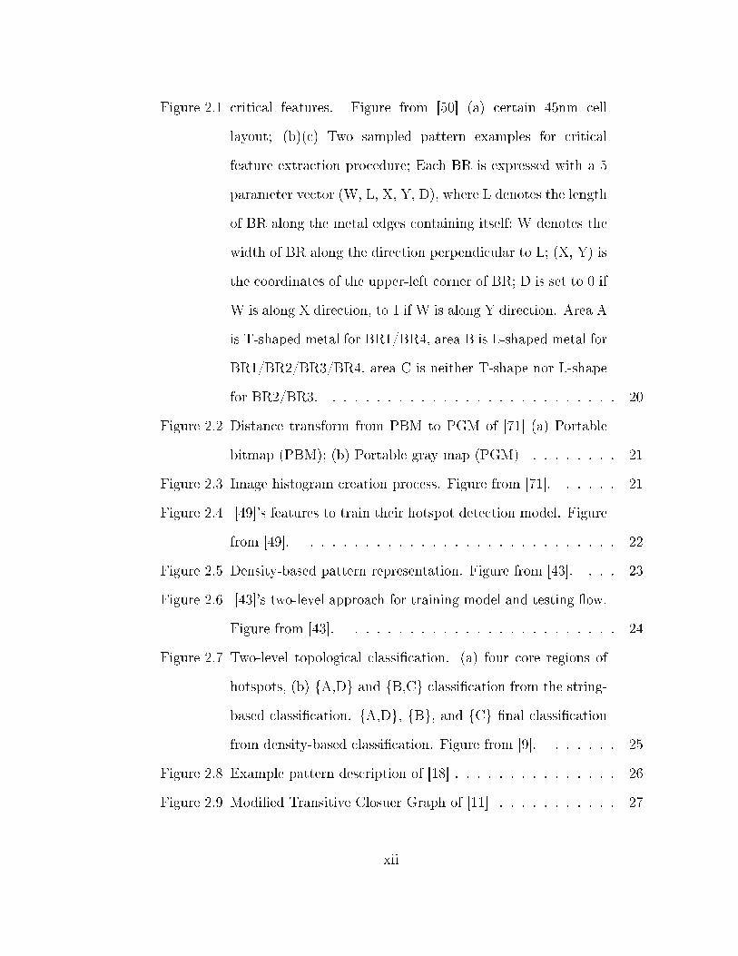


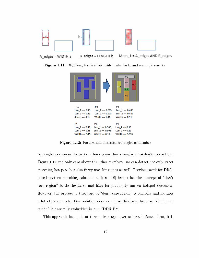


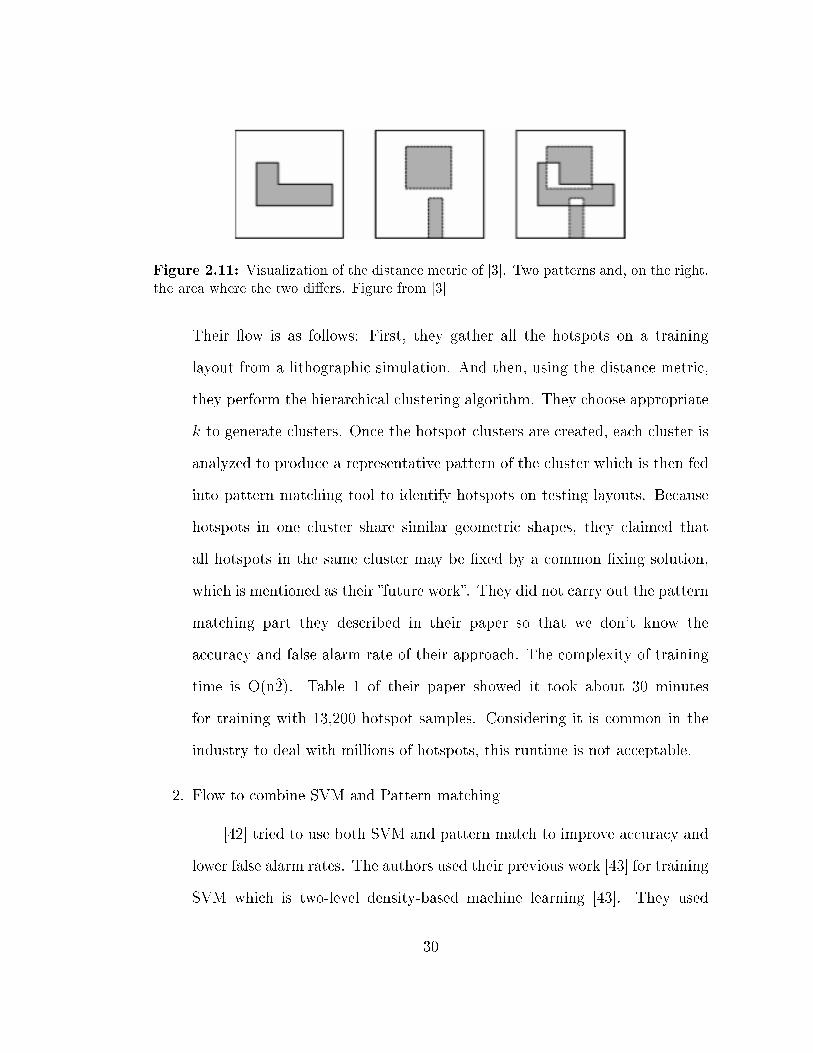


![2 LASER INTERFERENCE LITHOGRAPHY - uni-halle.de · 2 LASER INTERFERENCE LITHOGRAPHY (LIL) 9 2 LASER INTERFERENCE LITHOGRAPHY (LIL) Laser interference lithography [3~22] (LIL) is a](https://static.documents.pub/doc/80x56/5eae180eecc7e273a41a4e88/2-laser-interference-lithography-uni-hallede-2-laser-interference-lithography.jpg)


