Lithospheric layering in the NorthAmerican cratonHuaiyu Yuan1 & Barbara Romanowicz1
How cratons—extremely stable continental areas of the Earth’s crust—formed and remained largely unchanged for morethan 2,500 million years is much debated. Recent studies of seismic-wave receiver function data have detected a structuralboundary under continental cratons at depths too shallow to be consistent with the lithosphere–asthenosphere boundary, asinferred from seismic tomography and other geophysical studies. Here we show that changes in the direction of azimuthalanisotropy with depth reveal the presence of two distinct lithospheric layers throughout the stable part of the NorthAmerican continent. The top layer is thick (,150 km) under the Archaean core and tapers out on the surrounding Palaeozoicborders. Its thickness variations follow those of a highly depleted layer inferred from thermo-barometric analysis ofxenoliths. The lithosphere–asthenosphere boundary is relatively flat (ranging from 180 to 240 km in depth), in agreementwith the presence of a thermal conductive root that subsequently formed around the depleted chemical layer. Our findingstie together seismological, geochemical and geodynamical studies of the cratonic lithosphere in North America. They alsosuggest that the horizon detected in receiver function studies probably corresponds to the sharp mid-lithospheric boundaryrather than to the more gradual lithosphere–asthenosphere boundary.
Cratons are continental regions where the Earth’s crust has remainedlargely undeformed since Archaean times1. How they were formedand how they survived destruction over timescales of billions of yearsremains a subject of vigorous debate. Interestingly, the cratoniclithosphere (the crust and the uppermost mantle) presents severaldistinctive and intriguing geological and geophysical features.Diamonds are found only in cratons or at their borders2, seismicvelocities remain significantly higher than average down to at least200 km depth3, and heat flow is low4, indicating that the cratoniclithosphere must be thick and cold. Yet there is no observed positivegeoid anomaly above cratons5, whereas geochemical evidence frommantle xenoliths indicates lithosphere depletion through meltextraction6. This has led to the concept of the ‘tectosphere’7: thatthe thick, chemically distinct cratonic lithosphere floats high abovethe oceans and resists destruction by subduction, owing to its par-ticularly low density and high viscosity, which result in part fromdehydration.
It remains a challenge for geodynamicists to explain why thickcratonic keels have resisted progressive entrainment into the mantleby convection8. The chemically depleted core may be underlain andsurrounded by a thermal, conductive boundary layer8–10 that acts as abuffer zone and shields the lithosphere from excessive deformation11.
Determining the thickness of the lithosphere is itself a challenge.Thermally, the intersection of the conductive geotherm with the mantleadiabat defines the base of the lithosphere8,12. However, the thicknessof cratonic roots remains poorly defined by seismic tomography.Although thicknesses in excess of 300 km have been suggested, recentestimates, taking into account the effects of anisotropy on seismicvelocities, indicate values no larger than 200–250 km (ref. 3), in agree-ment with results from xenolith and xenocryst thermobarometry6,13,heat flow measurements4 and electrical conductivity data14. Yet receiverfunction studies, which are more sensitive to fine-scale structure, havelargely failed to detect the lithosphere–asthenosphere boundary (LAB)at these depths, indicating that it may not be a sharp boundary under-neath cratons. On the other hand, strong compressional-to-shear wave
(P–S) and shear-to-compressional wave (S–P) conversions have beenfound recently at shallower depths (100–140 km) under stable con-tinental regions15–17, leading some authors to infer that the cratoniclithosphere may be considerably thinner than expected15,17, contradict-ing tomographic and other geophysical or geochemical inferences. Thesimplest way to reconcile these results is to consider that the receiverfunction studies detect an intra-continental discontinuity rather thanthe LAB18. Such a discontinuity is consistently found in the analysis oflong-range seismic profiles19 and has been attributed to the presence ofa zone of partial melt and/or dehydration around depths of 100 km.Evidence for continental lithospheric layering is well documentedfrom a variety of local and regional studies20,21 (see also Supplemen-tary section 1).
Finally, there are two classes of competing hypotheses on the forma-tion of cratonic lithospheric roots12. The first one invokes underplat-ing by one or more hot plumes and the other invokes accretion byshallow subduction in either a continental or arc setting. The cratoniccores were probably formed under the very different tectonic regimeof a hotter Archaean mantle, which would have evolved to present-dayplate tectonics sometime in the late Archaean era2,6,22, as a con-sequence of secular cooling.
Two-layered lithosphere in the North American craton
The North American continent is particularly well suited to the studyof the question of lithospheric structure and thickness as a function ofage of the overlying crust, because of the presence of a well definedArchaean core surrounded by progressively younger Proterozoic andPalaeozoic provinces1,23 (Fig. 1a). Here we present the results of astudy of azimuthal anisotropy in the upper mantle beneath NorthAmerica and illustrate how the change with depth of the orientationof the fast axis of anisotropy provides a powerful tool for the detectionof layering in the upper mantle. Anisotropy in the upper mantle ismost probably caused by lattice preferred orientation24 and holds cluesto dynamical processes responsible for past and present deformation.
1Berkeley Seismological Laboratory, 209 McCone Hall, Berkeley, California 94720, USA.
Vol 466 | 26 August 2010 | doi:10.1038/nature09332
This study further refines the methodology developed by Maroneand Romanowicz25, and is based upon the joint inversion of long-period seismic waveforms and SKS wave splitting data, using here amuch larger data set, providing unprecedented lateral and depthresolution throughout the continent (Supplementary Figs 1 and 2).As shown in ref. 25, models obtained from surface waveforms with orwithout constraints from SKS splitting measurements reveal thesame variations with depth in the orientation of the fast axis ofazimuthal anisotropy, but the strength of anisotropy recovered atdepths greater than 200 km is larger with the SKS constraints, with-out degrading the fit to surface waves (see Methods and Supplemen-tary Figs 3, 4 and 5).
In ref. 25, we found that the fast axis of anisotropy systematicallychanges direction towards the direction of absolute plate motion(APM, as defined in the hotspot reference frame26) at a depth cor-responding to the LAB, throughout the North American continent.Here we confirm and refine these results, and we also find that, underthe craton, the fast axis of anisotropy changes direction significantlywith depth in the upper mantle, not only at around 200 km depth, butalso at a shallower depth between 50 and 160 km, depending on
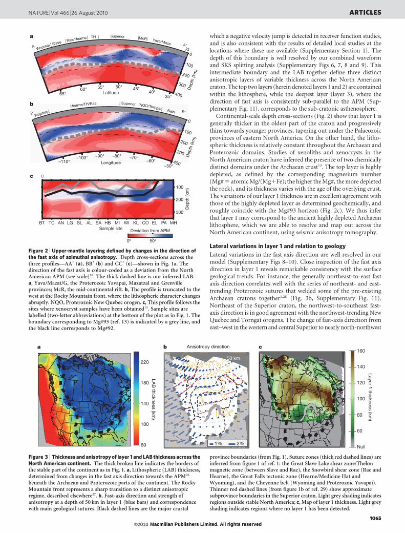
location (Figs 1b–e, 2). This defines two boundaries, each of whichis well localized in depth (within about 15 km) and is accompanied bya minimum in the amplitude of azimuthal anisotropy. We note thataround the depth of the deeper boundary, the depth profile of iso-tropic S-wave velocity (Vs) shows a pronounced negative gradient,but, in contrast to azimuthal anisotropy, it does not allow us to locatethe transition to better than 50–100 km in depth. Likewise, the radialanisotropy profiles show a gradual decrease with depth, but no loca-lized transition is resolved. We thus define the LAB as the laterallyvarying horizon marked by the change of fast axis with depth towardsthe APM (Figs 1b–e, 2, 3a). We note that, east and southeast of thecraton, the lithosphere remains thick well into provinces ofProterozoic age. West of the Rocky Mountain Front, on the otherhand, it becomes rapidly much thinner (Fig. 3a). We next focus onthe Proterozoic and Archaean parts of the continent, and defer furtherdiscussion of the tectonically active western part of North America to aseparate publication27.
Interestingly, the shallower horizon detected within the craton isoften accompanied by a local minimum in the isotropic shear velocity(Fig. 1b–e); this minimum generally falls within the depth range in
YKW3YKW3
Cordillera
BTBT
ELEL
MHMH
HBHB
LGLG
SlaveSlave
FCCFCC
ULMULM
Appal
achia
ns
SuperiorSuperior
Thelon
Thelon
RaeRae
NainNain
TH
Yavapai
Mazatzal
HearneHearne
WyomingWyoming
A
B
C
B′
C′
A′
CBCB
GFT
GFT
Grenville
NQONQO
Torngat
Torngat
Archaean
Proterozoic (2.0–1.85 billion years)
Proterozoic (1.8–1.6 billion years)
Proterozoic (1.3–1.0 billion years)
Mid-continental rift (1.1 billion years)
Xenocryst sample sites
Receiver function stations
Stable cratonic region
Depth cross-sections
Suture/shear zones
a b
c
d
e
50
100
150
200
250
300
350
50
100
150
200
250
300
350
50
100
150
200
250
300
350
50
100
150
200
250
300
350
Dep
th (km
)D
ep
th (km
)D
ep
th (km
)D
ep
th (km
)
Fast axis ζ d(InG) (%)Vs (m s–1)
N 4
5º W
N 4
5º EN
4,40
0
4,80
0
N 4
5º W
N 4
5º EN
4,40
0
4,80
0
1 1 201.04
1 1 201.04
N 4
5º W
N 4
5º EN
4,40
0
4,80
0 1 1 201.04
4,40
0
4,80
0 1N E S W 1 201.04
Snow
bird
Snow
bird
SASA
GSLGSL
SCHQSCHQ
Wopmay
Figure 1 | Precambrian basement age in the North American continent andseismic depth profiles at selected locations. a, Precambrian basement age(after ref. 23). The white triangles are the seismic stations used in b, and theblue lines are the locations of profiles AA9, BB9 and CC9, discussed in thetext. Petrologic sample locations are from ref. 13. The thick dashed black lineshows the approximate boundary of the stable parts of the continent,bounded by the Laramide deformation/Rocky Mountain front from thewest, and the Ouachita and Appalachian fronts from the south and east1. Thethick dashed grey lines indicate crustal shear zones1. GSL, the Great SlaveLake shear zone; GFT, the Great Falls tectonic zone; TH, the Trans-Hudsonorogen; CB, the Cheyenne belt; NQO and Torngat, shear zones related to theNew Quebec orogen and the Torngat orogen, respectively. Blue two-letterlabels are Xenocryst sample site names. b–e, Seismic depth profiles at
stations YKW3 (b), ULM (c), FFC (d) and SCHQ (e). Panels show, from leftto right, the direction of the fast axis of azimuthal anisotropy, isotropicshear-wave velocity (VS), radial anisotropy (j) and azimuthal anisotropymagnitude (G), respectively. The green dashed lines indicate local maxima inthe fast-axis direction gradient as a function of depth, and also delimit threeanisotropic layers. The gradient itself is shown as a red line in the fast-axispanels, and the vertical thin black lines denote the North American APMdirection26 at the station. (In c and d, there are two black lines, which showthe same APM directions owing to 180u periodicity.) Regions of negativegradients in VS and j are highlighted as thick blue rectangles. Changes inanisotropy direction at depths shallower than 50 km (d, e) are probablyartefacts at the edge of our inversion domain.
which a negative velocity jump is detected in receiver function studies,and is also consistent with the results of detailed local studies at thelocations where these are available (Supplementary Section 1). Thedepth of this boundary is well resolved by our combined waveformand SKS splitting analysis (Supplementary Figs 6, 7, 8 and 9). Thisintermediate boundary and the LAB together define three distinctanisotropic layers of variable thickness across the North Americancraton. The top two layers (herein denoted layers 1 and 2) are containedwithin the lithosphere, while the deepest layer (layer 3), where thedirection of fast axis is consistently sub-parallel to the APM (Sup-plementary Fig. 11), corresponds to the sub-cratonic asthenosphere.
Continental-scale depth cross-sections (Fig. 2) show that layer 1 isgenerally thicker in the oldest part of the craton and progressivelythins towards younger provinces, tapering out under the Palaeozoicprovinces of eastern North America. On the other hand, the litho-spheric thickness is relatively constant throughout the Archaean andProterozoic domains. Studies of xenoliths and xenocrysts in theNorth American craton have inferred the presence of two chemicallydistinct domains under the Archaean crust13. The top layer is highlydepleted, as defined by the corresponding magnesium number(Mg# 5 atomic Mg/(Mg1Fe); the higher the Mg#, the more depletedthe rock), and its thickness varies with the age of the overlying crust.The variations of our layer 1 thickness are in excellent agreement withthose of the highly depleted layer as determined geochemically, androughly coincide with the Mg#93 horizon (Fig. 2c). We thus inferthat layer 1 may correspond to the ancient highly depleted Archaeanlithosphere, which we are able to resolve and map out across theNorth American continent, using seismic anisotropy tomography.
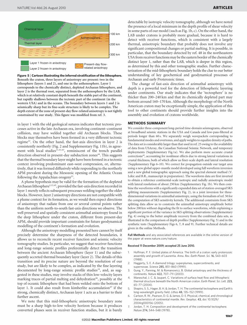
Lateral variations in layer 1 and relation to geology
Lateral variations in the fast axis direction are well resolved in ourmodel (Supplementary Figs 8–10). Close inspection of the fast axisdirection in layer 1 reveals remarkable consistency with the surfacegeological trends. For instance, the generally northeast-to-east fastaxis direction correlates well with the series of northeast- and east-trending Proterozoic sutures that welded some of the pre-existingArchaean cratons together1,28 (Fig. 3b, Supplementary Fig. 11).Northeast of the Superior craton, the northwest-to-southeast fast-axis direction is in good agreement with the northwest-trending NewQuebec and Torngat orogens. The change of fast-axis direction fromeast–west in the western and central Superior to nearly north-northwest
Figure 2 | Upper-mantle layering defined by changes in the direction ofthe fast axis of azimuthal anisotropy. Depth cross-sections across thethree profiles—AA9 (a), BB9 (b) and CC9 (c)—shown in Fig. 1a. Thedirection of the fast axis is colour-coded as a deviation from the NorthAmerican APM (see scale)26. The thick dashed line is our inferred LAB.a, Yava/Mazat/G, the Proterozoic Yavapai, Mazatzal and Grenvilleprovinces; McR, the mid-continental rift. b, The profile is truncated to thewest at the Rocky Mountain front, where the lithospheric character changesabruptly. NQO, Proterozoic New Quebec orogen. c, This profile follows thesites where xenocryst samples have been obtained13. Sample sites arelabelled (two-letter abbreviations) at the bottom of the plot as in Fig. 1. Theboundary corresponding to Mg#93 (ref. 13) is indicated by a grey line, andthe black line corresponds to Mg#92.
Null
60
80
100
120
140
160
1% 2%
a cb
50 km
Anisotropy direction
Layer 1
thic
kn
ess (k
m)
60
100
140
180
220
LA
B th
ickness (k
m)
Figure 3 | Thickness and anisotropy of layer 1 and LAB thickness across theNorth American continent. The thick broken line indicates the borders ofthe stable part of the continent as in Fig. 1. a, Lithospheric (LAB) thickness,determined from changes in the fast axis direction towards the APM26
beneath the Archaean and Proterozoic parts of the continent. The RockyMountain front represents a sharp transition to a distinct anisotropicregime, described elsewhere27. b, Fast-axis direction and strength ofanisotropy at a depth of 50 km in layer 1 (blue bars) and correspondencewith main geological sutures. Black dashed lines are the major crustal
province boundaries (from Fig. 1). Suture zones (thick red dashed lines) areinferred from figure 1 of ref. 1: the Great Slave Lake shear zone/Thelonmagnetic zone (between Slave and Rae), the Snowbird shear zone (Rae andHearne), the Great Falls tectonic zone (Hearne/Medicine Hat andWyoming), and the Cheyenne belt (Wyoming and Proterozoic Yavapai).Thinner red dashed lines (from figure 1b of ref. 29) show approximatesubprovince boundaries in the Superior craton. Light grey shading indicatesregions outside stable North America; c, Map of layer 1 thickness. Light greyshading indicates regions where no layer 1 has been detected.
in the northeastern Superior craton also follows the trends of the geo-logical sutures of the Superior province29. Fossil subductions, revealedas strong mantle reflectors and high-velocity bodies from active andpassive seismic studies30–32 are found beneath most of these suture zonesand generally indicate a subduction direction normal to the suturetrends. We note that the fast-axis directions in lithospheric layer 1and in the asthenosphere (layer 3) are comparable, similar both tosurface geological trends and to the APM (Fig. 1b–e, SupplementaryFig. 5). This suggests a resolution to the long-running controversysurrounding the interpretation of SKS splitting measurements in con-tinents in terms of frozen anisotropy33 versus anisotropy aligned withthe present-day flow34: azimuthal anisotropy in layer 1 reflects ancienttectonic events dating back to the late Archaean era, whereas sub-lithospheric anisotropy reflects present-day tectonics. They both con-tribute to SKS splitting.
The thickness of layer 1 varies from about 50 km south of the1.1-billion-year-old mid-continental rift to over 150 km beneaththe 1.8-billion-year-old Trans-Hudson orogen and the 1.9-billion-year-old Wopmay orogen1 (Fig. 3c). We note that the thickest part isnot in the region of oldest Archaean crust, but corresponds to theTrans-Hudson orogen, which has an arcuate shape, and mayhave been formed as part of the continental collision between theSuperior craton to the southeast and the Hearne and Rae cratons tothe northwest1. Indeed, the collisional processes of the Proterozoicera have been linked to those presently active in the India/Asia collisionzone along the Himalayas35, where the lithosphere is also thickened.Thicker parts of layer 1 are also found in the northwestern corner of ourregion, affected by the 1.9-billion-year-old Wopmay orogeny1. Thethickening of layer 1 may thus reflect the results of continental collisionin the late Archaean era. Layer 1 thins out and disappears on the easternborderlands of the continent, which have been subjected to Palaeozoicorogenies, and also west of the Rocky Mountain Front, which is subjectto even more recent and currently active tectonics. Within theProterozoic regions, layer 1 is thinnest near the 1.1-billion-year-oldmid-continental rift1, suggesting that the original Archaean lithospheremay have been perturbed subsequently by rifting. In the south, nolayer 1 is found in part of the Proterozoic Yavapai/Mazatzal province.On the eastern border of the craton, layer 1 is present in regions wherethe Proterozoic crust is underlain by Archaean upper mantle36,suggesting that the Archaean lithosphere is probably more laterallyextensive at depth than near the surface, and, in places, may be wedgedinto the more juvenile (Proterozoic province) blocks37. To infer morecompletely the patterns of anisotropy, and in particular the dip of theaxis of symmetry, azimuthal anisotropy needs to be combined withother information, including radial anisotropy38. Under the North
American craton, the velocity of horizontally polarized shear waves,VSH, exceeds that of vertically polarized shear waves, VSV, in general,indicating dominant horizontal shear39. However, significant radialanisotropy anomalies, with VSH , VSV, coincide with the location ofsome of the suture zones (such as the Rae/Hearne and Hearne/Trans-Hudson zones; see Supplementary Fig. 12b, e), suggesting the localpresence of anisotropy with dipping axis possibly related to fossilaccretion processes40. Resolving the dip of the axis involves makingstrong assumptions on the mineralogy, which is beyond the scope ofthis paper.
The nature of layer 2
Comparison with the geochemistry studies (Fig. 2c) suggests thatlayer 2 may represent a younger, less depleted, thermal boundarylayer, possibly accreted at a later stage through processes influencedby the presence of a stagnant, chemically distinct lid (layer 1). Thisscenario is supported by the excellent agreement between the lateralvariations in the depth of the LAB inferred from our azimuthalanisotropy study and the variations predicted from the thickness oflayer 1 (Fig. 4), when applying the geodynamically inferred relation-ship between the thicknesses of the chemical and thermal litho-spheres10,12. Except for a few locations at the margins of the cratonwhere layer 1 thins out, the overall misfit between the observed andpredicted LAB is 615 km. While the thickness of layer 1 varies sig-nificantly across the stable part of the continent, the lithosphere asdefined by the bottom of layer 2 is remarkably flat (depths between180 and 240 km), including in the Proterozoic provinces where layer 1has thinned out (Figs 3a, 4a), and as predicted by geodynamicalmodelling10. The flat LAB at the bottom of the thermal conductivelayer is also in good agreement with local seismic, petrologic andmagnetotelluric studies (Supplementary Section 2) and indicatesthe lack of strong lateral variations in temperature at greater depthsbelow the stable continent, in agreement with the absence of signifi-cant topography on the 400-km and 660-km discontinuities41. Whencombining azimuthal anisotropy and radial anisotropy results,shorter wavelength variations within layer 2 are observed, whichprobably hold additional clues on the formation of this layer (Sup-plementary Fig. 12).
Implications for the formation of continental lithosphere
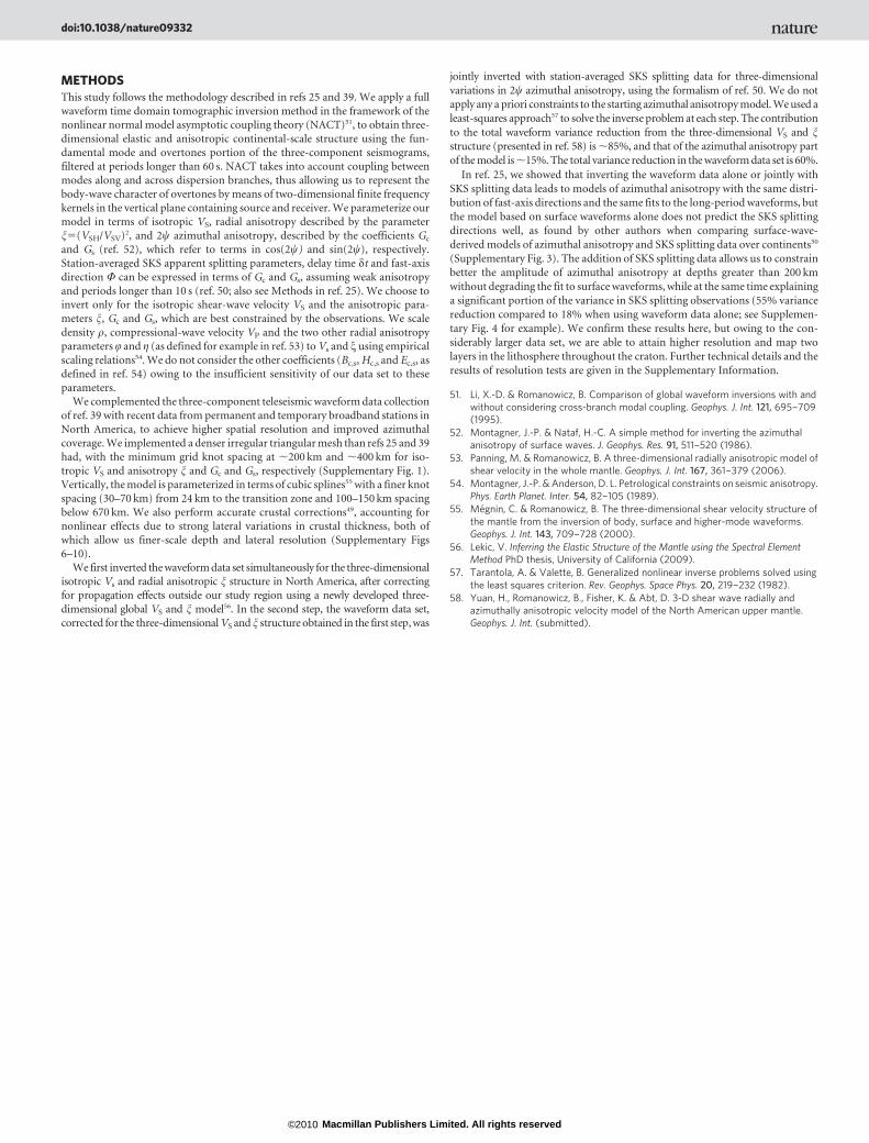
Here, by using an approach based on seismic azimuthal anisotropy,we have documented the craton-wide presence of a mid-lithosphericboundary, separating a highly depleted chemical layer of laterallyvarying thickness, from a less depleted deeper layer bounded belowby a relatively flat LAB (Fig. 5). Alignment of the fast anisotropy axis
Fast-axis direction gradient (º km–1)
−5 0 5
Layer 1 boundary
LAB measured
LAB predicted
Receiver function negativegradient phase depth
Latitude50
Dep
th (km
)
100 150 200
2
3
4
Chemical lithosphere (km)
Therm
al/chem
ical ra
tio
0
100
200
300
40035°40°
45°55°60°
65°
A A′Δ
Δ ΔYKW3
FFC ULMa b
50°
Figure 4 | Relative thickness of layers 1 and 2 along the depth cross-sectionAA’ shown in Figs 1a and 2a. a, Gradient of the fast-axis direction as afunction of depth along the profile. Gradient extremes mark the boundariesbetween layers 1 and 2 (white dashed line) and the LAB (continuous whiteline). The red dashed line is the prediction of LAB depth from the
geodynamic calculation10, according to the relation between thickness ofchemical (layer 1) and thermal (layer 1 1 layer 2) lithosphere (b), and usingas input our layer 1 thickness. This is in good agreement with the seismicallyinferred LAB north of 38u latitude. The black dots indicate depth ofboundary detected by receiver function studies15–17.
in layer 1 with the old geological sutures indicates that tectonic pro-cesses active in the late Archaean era, involving continent–continentcollision, may have welded together old Archaean blocks. Theseblocks may themselves have been formed in a very different tectonicregime22. On the other hand, the fast-axis direction in layer 2 isconsistently northerly (Fig. 2 and Supplementary Fig. 11b), in agree-ment with local studies21,42,43, reminiscent of the trench paralleldirection observed in present-day subduction zones44. This suggeststhat the thermal boundary layer might have been formed in a tectoniccontext involving predominant east–west compression, or, alterna-tively, that it was formed diffusively while responding to the northerlyAPM prevalent during the Mesozoic opening of the Atlantic Oceanfollowing the Appalachian orogeny21.
A plume hypothesis may be valid for the formation of the depletedArchaean lithosphere2,12,45, provided the fast-axis direction recorded inlayer 1 merely reflects subsequent processes welding together the olderblocks. However, layer 2 anisotropy directions are not compatible witha plume context for its formation, as we would then expect directionsof anisotropy that radiate from one or several central points ratherthan the uniform north-to-south fast-axis directions we observe. Thewell preserved and spatially consistent azimuthal anisotropy found inthe deep lithosphere under the craton, different from present-dayAPM, should provide important constraints for future geodynamicalmodelling of the continent’s formation and evolution.
Although the anisotropy modelling presented here cannot by itselfprecisely determine the sharpness of the detected boundaries, itallows us to reconcile recent receiver function and seismic velocitytomography studies. In particular, we suggest that receiver functionsand long-range seismic profiles preferentially detect the transitionbetween the ancient Archaean lithosphere (layer 1) and the subse-quently accreted thermal boundary layer (layer 2). The details of thistransition and its precise nature are beyond the resolution of ourstudy, but are likely to be complex, as indicated by the fine layeringdocumented by long-range seismic profile studies19, and, as sug-gested in these studies, may involve stacks of thin low-velocity layersmarking traces of partial melting and dehydration46, possibly at thetop of oceanic lithosphere that had been welded onto the bottom oflayer 1. It could also result from kimberlite accumulation47 if thestrong, chemically distinct, Archaean layer 1 acts as a barrier to theirfurther ascent.
We note that this mid-lithospheric anisotropic boundary zonemust be a sharp high-to-low velocity horizon because it producesconverted phases seen in receiver function studies, but it is barely
detectable by isotropic velocity tomography, although we have notedthe presence of a local minimum in the depth profile of shear velocityin some parts of our model (such as Fig. 1b, c). On the other hand, theLAB under cratons is probably more gradual, because it is hard todetect with receiver functions, which is consistent with a largelythermal, anisotropic boundary that probably does not involve anysignificant compositional changes or partial melting. It is possible, inparticular, that the boundary detected by ref. 48 in the northeasternUSA from receiver functions may be the eastern border of the chemicallydistinct layer 1, rather than the LAB, which is deeper in this region,as determined by this and other tomographic studies. Further charac-terization of the mid-lithospheric boundary holds the clue to our betterunderstanding of key geochemical and geodynamical processes ofArchaean and early Proterozoic times.
The change of fast-axis direction of azimuthal anisotropy withdepth is a powerful tool for the detection of lithospheric layeringunder continents. Our study indicates that the ‘tectosphere’ is nothicker than 200–240 km and that its chemically depleted part maybottom around 160–170 km. Although the morphology of the NorthAmerican craton may be exceptionally simple, the application of thistool to other continents should provide further insights into theassembly and evolution of cratons worldwide.
METHODS SUMMARY
We consider three-component long-period time-domain seismograms, observed
at broadband seismic stations in the USA and Canada and low-pass-filtered at
periods longer than 60 s. We separately weigh wavepackets corresponding to
fundamental modes and overtones, and apply weights to equalize density of paths.
The data set is considerably larger than that used in ref. 25 owing to the availability
of data from USArray, the Canadian National Seismic Network, and temporary
deployments (Supplementary Fig.1a). We also perform more accurate crustal
corrections49, accounting for nonlinear effects due to strong lateral variations in
crustal thickness, both of which allow us finer-scale depth and lateral resolution
(Supplementary Figs 6–10). We correct for propagation outside our target area
using a new global upper-mantle model developed using full waveform inversion
and a new global tomographic approach using the spectral element method (V.
Lekic and B.R., manuscript in preparation). The waveform data are first inverted
to obtain a reference continental-scale isotropic and radially anisotropic model
with lateral resolution of about 250 km (Supplementary Fig. 1b). We then com-
bine the waveforms with a significantly expanded data set of station-averaged SKS
splitting measurements (Supplementary Fig. 2), in a joint inversion for three-
dimensional variations in azimuthal anisotropy, using the formalism of ref. 50 for
the computation of SKS sensitivity kernels. The additional constraints from SKS
splitting data allow us to constrain the azimuthal anisotropy amplitude better
below 200 km without degrading the fit to surface waveforms, while explaining a
significant portion of the variance in SKS splitting observations (Supplementary
Fig. 4) owing to the better amplitude recovery from the combined data sets, as
illustrated in the comparison of depth profiles (Supplementary Fig. 5) and in the
synthetic tests (Supplementary Figs 6, 7, 8 and 9). Further technical details are
given in the online Methods.
Full Methods and any associated references are available in the online version ofthe paper at www.nature.com/nature.
Received 11 December 2009; accepted 25 June 2010.
1. Hoffman, P. F. United plates of America. The birth of a craton: early proterozoicassembly and growth of Laurentia. Annu. Rev. Earth Planet. Sci. 16, 543–603(1988).
2. Haggerty, S. E. A diamond trilogy: superplumes, supercontinents, andsupernovae. Science 285, 851–860 (1999).
3. Gung, Y., Panning, M. & Romanowicz, B. Global anisotropy and the thickness ofcontinents. Nature 422, 707–711 (2003).
4. Mareschal, J. C. & Jaupart, C. Variations of surface heat flow and lithosphericthermal structure beneath the North American craton. Earth Planet. Sci. Lett. 223,65–77 (2004).
5. Shapiro, S. S., Hager, B. H. & Jordan, T. H. The continental tectosphere and Earth’slong-wavelength gravity field. Lithos 48, 135–152 (1999).
6. Carlson, R. W., Pearson, D. G. & James, D. E. Physical, chemical, and chronologicalcharacteristics of continental mantle. Rev. Geophys. 43, doi: 10.1029/2004rg000156 (2005).
7. Jordan, T. H. Composition and development of the continental tectosphere.Nature 274, 544–548 (1978).
100 km
200 km
300 km
Chemical layer
Thermal layerLAB
Asthenosphere
Present-day flow-
related anisotropy
Layer 1 frozen-in anisotropy
Layer 2 frozen-in anisotropy
Figure 5 | Cartoon illustrating the inferred stratification of the lithosphere.Beneath the craton, three layers of anisotropy are present: two in thelithosphere (layers 1 and 2), and one in the asthenosphere. Layer 1corresponds to the chemically distinct, depleted Archaean lithosphere, andlayer 2 is the thermal root, separated from the asthenosphere by the LAB,which is at relatively constant depth beneath the stable part of the continent,but rapidly shallows between the tectonic part of the continent (in thewestern USA) and in the oceans. The boundary between layers 1 and 2 isseismically sharp but its fine-scale structure is likely to be complex. Thedepth extent of the zone of present-day flow-related anisotropy is not tightlyconstrained by our study. This figure was modified from ref. 3.
8. King, S. D. Archean cratons and mantle dynamics. Earth Planet. Sci. Lett. 234, 1–14(2005).
9. Sleep, N. H. Survival of Archean cratonal lithosphere. J. Geophys. Res. 108, doi:10.1029/2001jb000169 (2003).
10. Cooper, C. M., Lenardic, A. & Moresi, L. The thermal structure of stablecontinental lithosphere within a dynamic mantle. Earth Planet. Sci. Lett. 222,807–817 (2004).
11. Lenardic, A., Moresi, L. & Muhlhaus, H. The role of mobile belts for the longevity ofdeep cratonic lithosphere: the crumple zone model. Geophys. Res. Lett. 27, doi:10.1029/1999gl008410 (2000).
12. Lee, C. T. in Archean Geodynamics and Environments (eds Benn, K. Mareschal, J. C.& Condie, K. C.) 89–114 (American Geophysical Union Monograph, 2006).
13. Griffin, W. L. et al. Lithosphere mapping beneath the North American plate. Lithos77, 873–922 (2004).
14. Jones, A. G. et al. The electrical structure of the Slave craton. Lithos 71, 505–527(2003).
15. Rychert, C. A. & Shearer, P. M. A global view of the lithosphere-asthenosphereboundary. Science 324, 495–498 (2009).
16. Abt, D. et al. North American lithospheric discontinuity structure imaged by Psand Sp receiver functions. J. Geophys. Res. doi: 10.1029/2009JB006710 (in thepress).
17. Yuan, X., Kind, R., Xueqing, L. & Rongjiang, W. The S receiver functions: syntheticsand data example. Geophys. J. Int. 165, 555–564 (2006).
18. Romanowicz, B. The thickness of tectonic plates. Science 324, 474–476 (2009).19. Thybo, H. & Perchuc, E. The seismic 8u discontinuity and partial melting in
continental mantle. Science 275, 1626–1629 (1997).20. Levin, V., Menke, W. & Park, J. Shear wave splitting in the Appalachians and the
Urals; a case for multilayered anisotropy. J. Geophys. Res. 104, 17975–17994(1999).
21. Deschamps, F., Lebedev, S., Meier, T. & Trampert, J. Stratified seismic anisotropyreveals past and present deformation beneath the East-central United States.Earth Planet. Sci. Lett. 274, 489–498 (2008).
22. Griffin, W. L. et al. The origin and evolution of Archean lithospheric mantle.Precambr. Res. 127, 19–41 (2003).
23. Canil, D. Canada’s craton: a bottom’s-up view. GSA Today 18, 4–11 (2008).24. Babuska, V. & Cara, M. Seismic Anisotropy in the Earth Ch. 5 (Kluwer Academic,
1991).25. Marone, F. & Romanowicz, B. The depth distribution of azimuthal anisotropy in
the continental upper mantle. Nature 447, 198–201 (2007).26. Gripp, A. E. & Gordon, R. G. Young tracks of hotspots and current plate velocities.
Geophys. J. Int. 150, 321–361 (2002).27. Yuan, H. & Romanowicz, B. Depth dependent azimuthal anisotropy in the western
US upper mantle. Earth Planet. Sci. Lett. (submitted).28. Whitmeyer, S. J. & Karlstrom, K. E. Tectonic model for the Proterozoic growth of
North America. Geosphere 3, 220–259 (2007).29. Percival, J. A. et al. Tectonic evolution of the western Superior Province from
NATMAP and Lithoprobe studies. Can. J. Earth Sci. 43, doi: 10.1139/E1106-1062(2006).
30. van der Velden, A. J. & Cook, F. A. Relict subduction zones in Canada. J. Geophys.Res. 110, doi: 10.1029/2004jb003333 (2005).
31. Bostock, M. G. Mantle stratigraphy and evolution of the Slave Province. J. Geophys.Res. 103, 21183–21200 (1998).
32. Yuan, H. & Dueker, K. in The Rocky Mountain Region—An Evolving Lithosphere:Tectonics, Geochemistry, and Geophysics (eds Randy, G. & Karlstrom, K. E.)Geophysical monograph 154, 329–345 (American Geophysical Union, 2005).
33. Silver, P. G. & Chan, W. W. Shear wave splitting and subcontinental mantledeformation. J. Geophys. Res. 96, 16429–16454 (1991).
34. Vinnik, L. P., Makeyeva, L. I., Milev, A. & Usenko, A. Y. Global patterns of azimuthalanisotropy and deformations in the continental mantle. Geophys. J. Int. 111,433–447 (1992).
35. St-Onge, M. R., Wodicka, N. & Ijewliw, O. Polymetamorphic evolution of theTrans-Hudson orogen, Baffin Island, Canada: integration of petrological,structural and geochronological data. J. Petrol. 48, 271–302 (2007).
36. Culotta, R. C., Pratt, T. & Oliver, J. A tale of two sutures: COCORP’s deep seismicsurveys of the Grenville province in the eastern U.S. midcontinent. Geology 18,646–649 (1990).
37. Snyder, D. B. Lithospheric growth at margins of cratons. Tectonophysics 355, 7–22(2002).
38. Montagner, J.-P. & Nataf, H.-C. Vectorial tomography. I. Theory. Geophys. J. 94,295–307 (1988).
39. Marone, F., Gung, Y. & Romanowicz, B. Three-dimensional radial anisotropicstructure of the North American upper mantle from inversion of surfacewaveform data. Geophys. J. Int. 171, 206–222 (2007).
40. Plomerova, J. & Babuska, V. Long memory of mantle lithosphere fabric—EuropeanLAB constrained from seismic anisotropy. Lithosdoi: 10.1016/j.lithos.2010.1001.1008 (in the press).
41. Li, A., Fischer, K. M., Wysession, M. E. & Clarke, T. J. Mantle discontinuities andtemperature under the North American continental keel. Nature 395, 160–163(1998).
42. Darbyshire, F. A. & Lebedev, S. Rayleigh wave phase-velocity heterogeneity andmultilayered azimuthal anisotropy of the Superior Craton, Ontario. Geophys. J. Int.176, 215–234 (2009).
43. Li, A., Forsyth, D. W. & Fischer, K. M. Shear velocity structure and azimuthalanisotropy beneath eastern North America from Rayleigh wave inversion. J.Geophys. Res. 108, doi: 10.1029/2002JB002259 (2003).
44. Long, M. D. & Silver, P. G. The subduction zone flow field from seismic anisotropy:a global view. Science 319, 315–318 (2008).
45. Arndt, N. T., Coltice, N., Helmstaedt, H. & Gregoire, M. Origin of Archeansubcontinental lithospheric mantle: some petrological constraints. Lithos 109,61–71 (2009).
46. Mierdel, K., Keppler, H., Smyth, J. R. & Langenhorst, F. Water solubility inaluminous orthopyroxene and the origin of Earth’s asthenosphere. Science 315,364–368 (2007).
47. Sleep, N. H. Stagnant lid convection and carbonate metasomatism of the deepcontinental lithosphere. Geochem. Geophys. Geosyst. 10,doi: 10.1029/2009gc002702 (2009).
48. Rychert, C. A., Fischer, K. M. & Rondenay, S. A sharp lithosphere–asthenosphereboundary imaged beneath eastern North America. Nature 436, 542–545 (2005).
49. Lekic, V. & Romanowicz, B. A simple method for improving crustal corrections inwaveform tomography. Geophys. J. Int. 182, 265–278 (2010).
50. Montagner, J.-P., Griot-Pommera, D.-A. & Lave, J. How to relate body wave andsurface wave anisotropy? J. Geophys. Res. 105, 19015–19027 (2000).
Supplementary Information is linked to the online version of the paper atwww.nature.com/nature.
Acknowledgements We thank the IRIS Data Management Center, the GeologicalSurvey of Canada and the Northern California Earthquake Data Center forproviding the waveform data used in this study. Discussion with K. Fischer helpedimprove the manuscript. We thank K. Liu, R. Allen, M. Fouch, A. Frederiksen andA. Courtier for providing their SKS compilations, and W. Griffin and S. O’Reilly fortheir North American olivine composition measurements. This study wassupported by a grant from the National Science Foundation/EarthScopeprogramme. This is the Berkeley Seismological Laboratory contribution number10-08.
Author Contributions B.R. developed the concept and methodology of the study.H.Y. assembled the data set, and performed the inversions and the supportingresolution tests. Both authors extensively discussed the results and jointlydeveloped implications. Both authors contributed to writing the paper.
Author Information Reprints and permissions information is available atwww.nature.com/reprints. The authors declare no competing financial interests.Readers are welcome to comment on the online version of this article atwww.nature.com/nature. Correspondence and requests for materials should beaddressed to B.R. ([email protected]).
METHODSThis study follows the methodology described in refs 25 and 39. We apply a full
waveform time domain tomographic inversion method in the framework of the
nonlinear normal model asymptotic coupling theory (NACT)51, to obtain three-
dimensional elastic and anisotropic continental-scale structure using the fun-
damental mode and overtones portion of the three-component seismograms,
filtered at periods longer than 60 s. NACT takes into account coupling between
modes along and across dispersion branches, thus allowing us to represent the
body-wave character of overtones by means of two-dimensional finite frequency
kernels in the vertical plane containing source and receiver. We parameterize our
model in terms of isotropic VS, radial anisotropy described by the parameter
j5(VSH/VSV)2, and 2y azimuthal anisotropy, described by the coefficients Gc
and Gs (ref. 52), which refer to terms in cos(2y) and sin(2y), respectively.
Station-averaged SKS apparent splitting parameters, delay time dt and fast-axis
direction W can be expressed in terms of Gc and Gs, assuming weak anisotropy
and periods longer than 10 s (ref. 50; also see Methods in ref. 25). We choose toinvert only for the isotropic shear-wave velocity VS and the anisotropic para-
meters j, Gc and Gs, which are best constrained by the observations. We scale
density r, compressional-wave velocity VP and the two other radial anisotropy
parameters Q and g (as defined for example in ref. 53) to Vs and j using empirical
scaling relations54. We do not consider the other coefficients (Bc,s, Hc,s and Ec,s, as
defined in ref. 54) owing to the insufficient sensitivity of our data set to these
parameters.
We complemented the three-component teleseismic waveform data collection
of ref. 39 with recent data from permanent and temporary broadband stations in
North America, to achieve higher spatial resolution and improved azimuthal
coverage. We implemented a denser irregular triangular mesh than refs 25 and 39
had, with the minimum grid knot spacing at ,200 km and ,400 km for iso-
tropic VS and anisotropy j and Gc and Gs, respectively (Supplementary Fig. 1).
Vertically, the model is parameterized in terms of cubic splines55 with a finer knot
spacing (30–70 km) from 24 km to the transition zone and 100–150 km spacing
below 670 km. We also perform accurate crustal corrections49, accounting for
nonlinear effects due to strong lateral variations in crustal thickness, both of
which allow us finer-scale depth and lateral resolution (Supplementary Figs
6–10).We first inverted the waveform data set simultaneously for the three-dimensional
isotropic Vs and radial anisotropic j structure in North America, after correcting
for propagation effects outside our study region using a newly developed three-
dimensional global VS and j model56. In the second step, the waveform data set,
corrected for the three-dimensional VS and j structure obtained in the first step, was
jointly inverted with station-averaged SKS splitting data for three-dimensional
variations in 2y azimuthal anisotropy, using the formalism of ref. 50. We do not
apply any a priori constraints to the starting azimuthal anisotropy model. We used a
least-squares approach57 to solve the inverse problem at each step. The contribution
to the total waveform variance reduction from the three-dimensional VS and jstructure (presented in ref. 58) is ,85%, and that of the azimuthal anisotropy part
of the model is ,15%. The total variance reduction in the waveform data set is 60%.
In ref. 25, we showed that inverting the waveform data alone or jointly with
SKS splitting data leads to models of azimuthal anisotropy with the same distri-
bution of fast-axis directions and the same fits to the long-period waveforms, but
the model based on surface waveforms alone does not predict the SKS splitting
directions well, as found by other authors when comparing surface-wave-
derived models of azimuthal anisotropy and SKS splitting data over continents50
(Supplementary Fig. 3). The addition of SKS splitting data allows us to constrain
better the amplitude of azimuthal anisotropy at depths greater than 200 km
without degrading the fit to surface waveforms, while at the same time explaining
a significant portion of the variance in SKS splitting observations (55% variance
reduction compared to 18% when using waveform data alone; see Supplemen-
tary Fig. 4 for example). We confirm these results here, but owing to the con-
siderably larger data set, we are able to attain higher resolution and map two
layers in the lithosphere throughout the craton. Further technical details and the
results of resolution tests are given in the Supplementary Information.
51. Li, X.-D. & Romanowicz, B. Comparison of global waveform inversions with andwithout considering cross-branch modal coupling. Geophys. J. Int. 121, 695–709(1995).
52. Montagner, J.-P. & Nataf, H.-C. A simple method for inverting the azimuthalanisotropy of surface waves. J. Geophys. Res. 91, 511–520 (1986).
53. Panning, M. & Romanowicz, B. A three-dimensional radially anisotropic model ofshear velocity in the whole mantle. Geophys. J. Int. 167, 361–379 (2006).
54. Montagner, J.-P. & Anderson, D. L. Petrological constraints on seismic anisotropy.Phys. Earth Planet. Inter. 54, 82–105 (1989).
55. Megnin, C. & Romanowicz, B. The three-dimensional shear velocity structure ofthe mantle from the inversion of body, surface and higher-mode waveforms.Geophys. J. Int. 143, 709–728 (2000).
56. Lekic, V. Inferring the Elastic Structure of the Mantle using the Spectral ElementMethod PhD thesis, University of California (2009).
57. Tarantola, A. & Valette, B. Generalized nonlinear inverse problems solved usingthe least squares criterion. Rev. Geophys. Space Phys. 20, 219–232 (1982).
58. Yuan, H., Romanowicz, B., Fisher, K. & Abt, D. 3-D shear wave radially andazimuthally anisotropic velocity model of the North American upper mantle.Geophys. J. Int. (submitted).