Llansó Diaz - Old Dominion...

OLD DOMINION UNIVERSITY 1Department of Biological Sciences Old Dominion University, Norfolk, Virginia 23529 2Versar, Incorporated 9200 Rumsey Road, Columbia, Maryland 21045 3Virginia Institute of Marine Science College of William and Mary, Gloucester Pt., Virginia, 23062 Preliminary evaluations of secondary productivity estimates as indicators of the ecological value of the benthos to higher trophic levels in Chesapeake Bay Prepared by Principal Investigators: Daniel M. Dauer1 Michael F. Lane1 Roberto J. Llansó2 Robert Diaz3 Submitted to: Virginia Department of Environmental Quality 629 East Main Street Richmond, Virginia 23230 December, 2011

CONTENTS

INTRODUCTION ............................................................................................................................... 2

METHODS ........................................................................................................................................ 3

Probability-based monitoring ..................................................................................................... 3

Benthic Secondary Production.................................................................................................... 4

RESULTS AND DISCUSSION ............................................................................................................. 5

Comparison of Edgar’s versus Brey’s estimates of benthic secondary productivity .................. 5

Benthic productivity - patterns and relationships with physic-chemical and benthic metrics .. 5

B-IBI Habitat Types .................................................................................................................. 5

CBP Benthic Monitoring Strata ............................................................................................... 6

CBP monitoring Segments ....................................................................................................... 6

CBP monitoring Segments - Low DO and Contaminant Effects .............................................. 7

Low Dissolved Oxygen and CBP Segment Benthic Productivity ................................................. 7

Sediment Contaminants and CBP Segment Benthic Productivity .............................................. 8

SUMMARY ....................................................................................................................................... 9

LITERATURE CITED ........................................................................................................................ 10

Dauer et al. 2011 Chesapeake Bay Benthic Secondary Productivity

1

INTRODUCTION Benthic macrofauna are important components of estuaries because they affect the physical and chemical properties of the sediment and water column, influence nutrient cycling, are food sources for higher trophic levels, are themselves commercially important and because their sedentary nature and life history characteristics expose them directly to both natural and man-made disturbances making them good indicators of those effects on estuarine systems (Reish, 1973; Boesch, 1973; Boesch, 1977; Pearson and Rosenberg,1978; Bilyard, 1987; Gray, et al., 1988; Dauer, 1993). As a result, a common approach to environmental assessment in estuarine systems is to develop indicators of macrobenthic community health that are measures of diversity, abundance, biomass and/or metrics related to sensitive or tolerant macrobenthic species (see review by Borja and Dauer, 2008). Such assessments, however, rarely involve evaluations of benthic secondary production (Dolbeth et al., 2010). Macrobenthic secondary production can be defined as the amount of organic matter incorporated into macrobenthic (>0.5mm) invertebrates per unit time and typically expressed per unit area. As such, these estimates would represent the amount of energy processed by these organisms from organic detritus and other sources and made available to higher trophic levels such as, crabs, bottom-feeding fish, diving ducks and shallow-water foraging birds. With respect to environmental management, measures of secondary production can be used to assess (1) the value of benthos as a food source for higher trophic levels (Asmus, 1987; Franz and Tanacredi, 1992; Tumbiolo and Downing, 1994; Wilson, 2002; Cusson and Bourget, 2005; Dolbeth et al., 2010); (2) the effects of anthropogenic inputs such loads of nutrients, sediment and contaminants on benthic communities (Steimle, 1985; Dolbeth 2003; Dolbeth 2007; Dauer et al. 2000; Bolam et al., 2011); (3) the efficacy of restoration and environmental management (Borja et al. 2008, 2010, 2011) particularly in an adaptive management and adaptive monitoring sense (Borja and Dauer, 2008); and (4) the impacts of climate change on macrobenthic communities (Dolbeth et al., 2007). The primary objective of this project was to develop an analytical tool that management could use to assess the ecological value of the benthos for higher trophic levels. Ideally any tool developed should be simple to implement, adaptable to both fixed and probability monitoring programs and applicable across multiple spatial and temporal scales. Direct evaluations of secondary productivity involve time-consuming cohort or size-based methods that require multiple measurements of the populations in question over time (Dolbeth et al., 2005; Cusson and Bourget, 2005). However, empirical regression models have been developed that provide reasonable alternatives to these techniques when direct measurements are not an option (e.g Schwinghamer et al., 1986; Edgar, 1990; Tumbiolo and Downing, 1994; Brey, 1999; Brey, 2001). These relationships incorporate benthic population metrics biomass, abundance, mean individual weights, etc.), environmental metrics (temperature, water depth), and taxon-specific metrics to adjust for body-size dependent turn-over rates to estimate production rates (or P/B ratios can be used to obtain production rates). Of the available empirical relationships we evaluated two approaches to calculate benthic secondary production in Chesapeake Bay – those of Edgar (1990) and Brey (2001) described in detail in the Methods section. Edgar’s


2

(1990) equation was selected because it has been used in several other studies conducted in Chesapeake Bay (Diaz and Schaffner 1990) and elsewhere (Wilbur and Clarke, 1998; Gillet, 2011; Kersey, 2011). Brey’s (2001) equation was selected because it incorporates variation related not only to temperature but also to sample depth and to effects relating to taxonomic composition that were not incorporated into Edgar’s model and because comparisons of different empirical models found that Brey’s model generally performed better than others (Dolbeth et al., 2005; Cusson and Bourget, 2005; Bolam et al., 2011). Finally, both of these equations can be easily calculated using data directly available from existing Chesapeake Bay Program data sets. This study presents our preliminary evaluations of both of these allometric equations for use in developing an assessment tool using benthic secondary production in Chesapeake Bay. We present estimates of average rates of secondary production at three spatial scales for the entire tidal portion of the Chesapeake Bay watershed as follows: (1) the 7 different B-IBI Weisberg habitat types (see Weisberg, et al., 1997); (2) the ten benthic sampling strata of the stratified-random benthic of the monitoring program in Chesapeake Bay (see Dauer and Llansó 2003) - plus an eleventh stratum from aggregated sites collected in the Elizabeth River watershed; and (3) the 73 Chesapeake Bay Program segments used a management tool to report overall condition in specific regions (i.e. 305(b)/303(d) reporting) (see, Llansó et al., 2009). Results from both equations were compared to values in the literature from Chesapeake Bay and similar estuaries. Our intent is to develop a benthic secondary productivity assessment tool to help in assessing ecological status patterns using the Benthic Index of Biotic I (B-IBI) (Weisberg et al., 1997). The B-IBI has been used effectively in Chesapeake Bay to: (1) identify impaired waters for Federally mandated management reports (Llansó et al., 2009); (2) estimate the extent of areal degradation of the watershed (Dauer and Llansó, 2003); and (3) relate benthic community condition to water quality, sediment quality and watershed stressors on a bay-wide scale (Dauer et al., 2000). We believe that complimentary studies investigating benthic secondary production will enhance adaptive management strategies at multiple spatial scales both for macrobenthic communities and higher trophic levels. METHODS Probability-based monitoring This study presents samples collected as part of the Chesapeake Bay Program’s probability-based benthic monitoring program from 1996 through 2009 coupled with probability-based samples collected as part of Virginia DEQ’s Elizabeth River Monitoring Program conducted from 1999 through 2007. The Chesapeake Bay Program allocated samples by assigning 25 random locations on an annual basis into 10 separate strata: (1) three in the Chesapeake Bay Mainstem; (2) five in major tributaries to the Mainstem; (3) two in Maryland eastern and western shore tributaries (see Dauer and Llansó 2003). For the Elizabeth River Monitoring Program, the main


3

sampling strata corresponded to main subwatersheds of the Elizabeth River i.e Western, Southern, and Eastern branches, the Lafayette River, the Elizabeth River Mainstem, as well as, several small contaminated tidal creeks sampled as additional strata during 1999 and 2002 (Dauer 2000, 2009). As with the CBP 25 random locations were assigned on an annual basis to each stratum. All samples were collected during the Benthic IBI index period (Weisberg et al., 1997) using a Young grab with a surface area of 440 cm2. Each sample was sieved on a 0.5 mm screen and preserved in the field. Samples were sorted, enumerated and identified to the lowest possible taxon. Ash-free dry weight biomass was determined for each taxon. Benthic Secondary Production We assessed the applicability of two general allometric equations as indicators of benthic secondary production. The first was that of Edgar (1990) which relates per sample daily macrobenthic production P to per sample standing crop biomass B in mg ash free dry weight (AFDW) and water temperature T in C as follows P = 0.0049 × B 0.80 T 0.89 Daily per sample estimates of production in g C were estimated for each individual taxon in the community and then summed across all taxa to obtain a daily total community production rate. Daily production rates were converted to annual rates per m2 by first multiplying the daily rates by 365 d/yr and dividing the result by the total area of the sample in m2 to obtain g C/m2/yr. The second equation used was a modified version of Brey’s (2001) formula for estimating P/B ratios based on mean body mass per individual w expressed in kJ, sample depth D in meters, temperature in K and several discrete (dummy) variables which took the following form: log10 (P/B) = 7.947 -2.294 × log10 (w) - (2409.856 × 1/T) + (0.168 × 1/D) + (0.194 × Subtid) + (0.180 × InfEpi ) + (0.174 × Tax1) - (0.188 × Tax2 ) + (0.330 × Tax3) + (582.851 × log10 (w) × 1/T) Subtid is a dummy variable that increases the P/B ratio if the organism is found in a subtidal habitat (i.e. a depth of > 1 meter) while InfEpi is set to 1 if the organism is infaunal also resulting in an increase in the P/B ratio. Tax1, Tax2 and Tax3 are dummy variables that identify specific effects on P/B ratio associated with membership in different taxonomic groups and that are set to 1 if the organism is: (1) an annelid or crustacean; (2) an echinoderm or (3) an insect, respectively, and 0 if otherwise. These terms result in an increase in P/B ratio for annelids, crustacean and insect species and a decrease in P/B ratio for echinoderm species. The original version of the formula includes additional dummy variable terms that do not apply to the samples collected in this study (e.g. regarding epifaunal mobility and lake habitat effects.


4

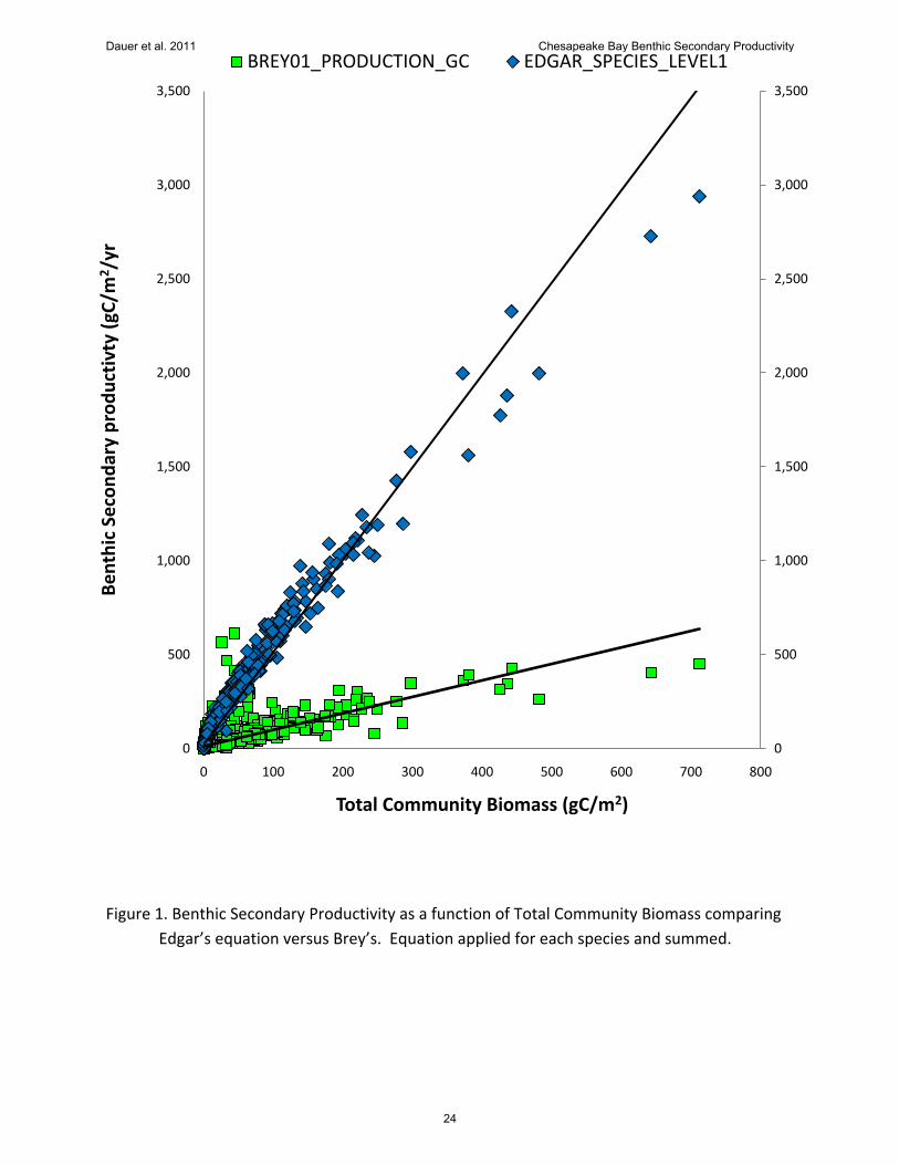
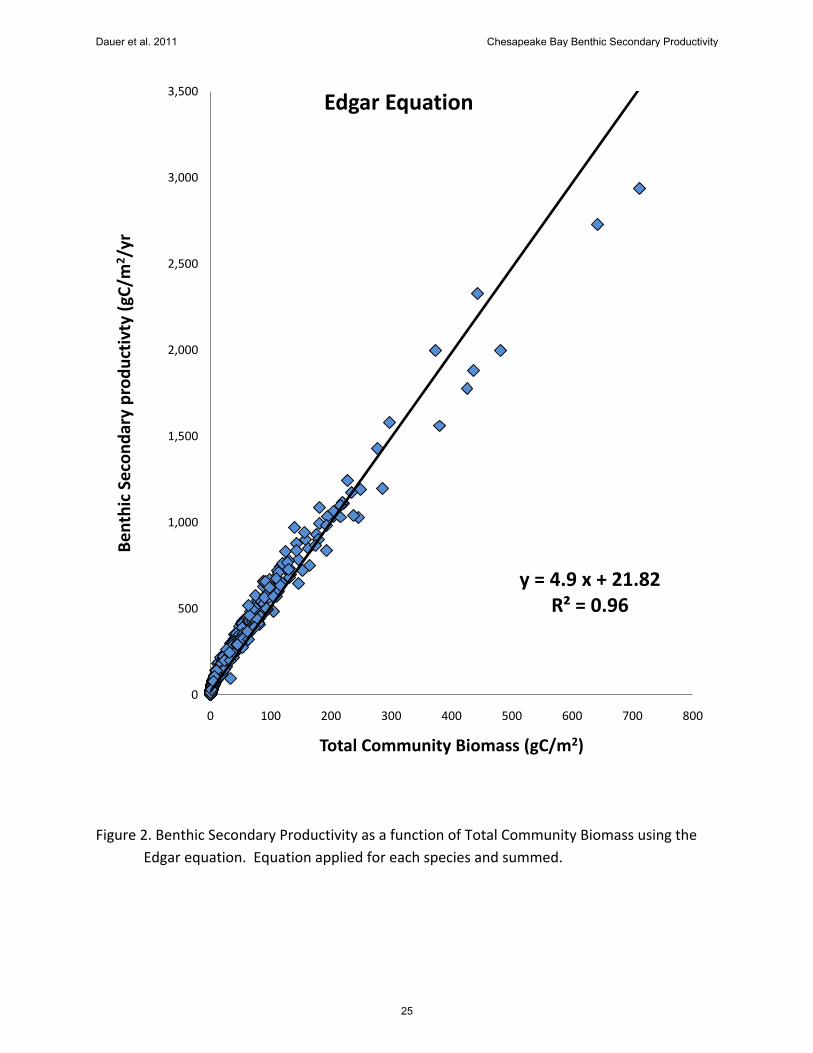
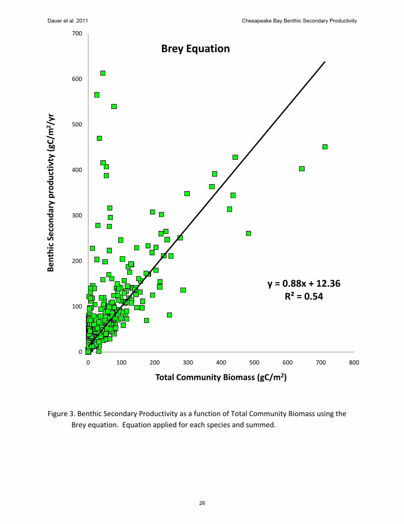
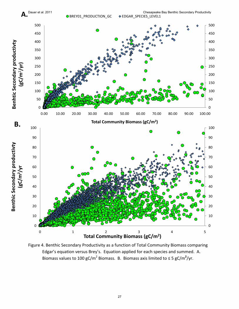
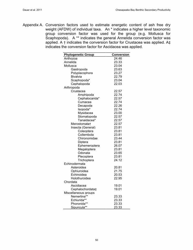
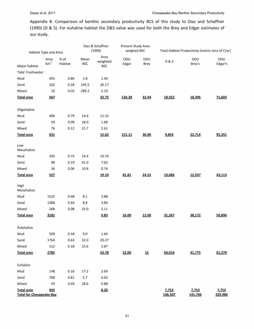
P/B ratios for individual species were estimated by first dividing the AFDW per sample by the total number of individuals to obtain an average mass per individual in g C. These values were then converted to the required units (kJ) using taxonomic group specific conversion factors provided by Brey (2001) (see Appendix A). The species level mass values in combination with depth and temperature recorded at the time of collection were used to calculate log10 transformed P/B ratios using the equation. By converting the ratio back to a linear scale (i.e. raising as an exponent to 10), the linear P/B ratios obtained were then multiplied to the mean standing crop biomass (per m2) to obtain an estimate of production per unit area and time for each species. We assumed that the standing crop values per sample were representative of one year of benthic community biomass and that the resultant productivity estimates were in units of g C/m2/yr for each species. Total community production for a given site was the summation of all taxa specific production values. RESULTS AND DISCUSSION Comparison of Edgar versus Brey estimates of benthic secondary productivity Edgar secondary productivity estimates were generally higher than those of the Brey estimates (Figure 1). The Edgar estimates of productivity were linearly related to biomass with an R2 value of 0.96 (Figure 2). Brey estimates were poorly related to biomass in a liner manner with an R2 = 0.54 (Figure 3). Benthic biomass values in Chesapeake Bay are not typically greater than 100 gC/m2 . Biomass values > 100 gC/m2 (Figure 4A) again show Edgar values for secondary productivity much higher the Brey values with the same pattern for biomass values > 5 gC/m2 that account for the vast majority of biomass values in Chesapeake. In essence Edgar values for benthic secondary productivity are basically a simple linear transformation of biomass values. For macrobenthic communities that contain species (1) with a diversity of life spans, (2) very different allocations of energy into protective coverings or ther refugia from predation (e.g. high versus low mobility), and (3) taxon-specific differences in P/B ratios that are best explained by natural history traits (Cusson and Bourget, 2005), the linear relationship to biomass of the Edgar values seems ecologically unreasonable. In addition the Brey equation contains many more variables than Edgar’s equation that are likely to affect secondary productivity and Brey values are more consistent with the review of production marine benthic habitats of Cusson and Bourget (2005). Finally our results Brey values were also consistent with estimates provided by Diaz and Schaffner (1990) for various benthic habitat types in Chesapeake Bay (see Appendix B). As such, further results of secondary production presented will be from Brey’s equation.


5

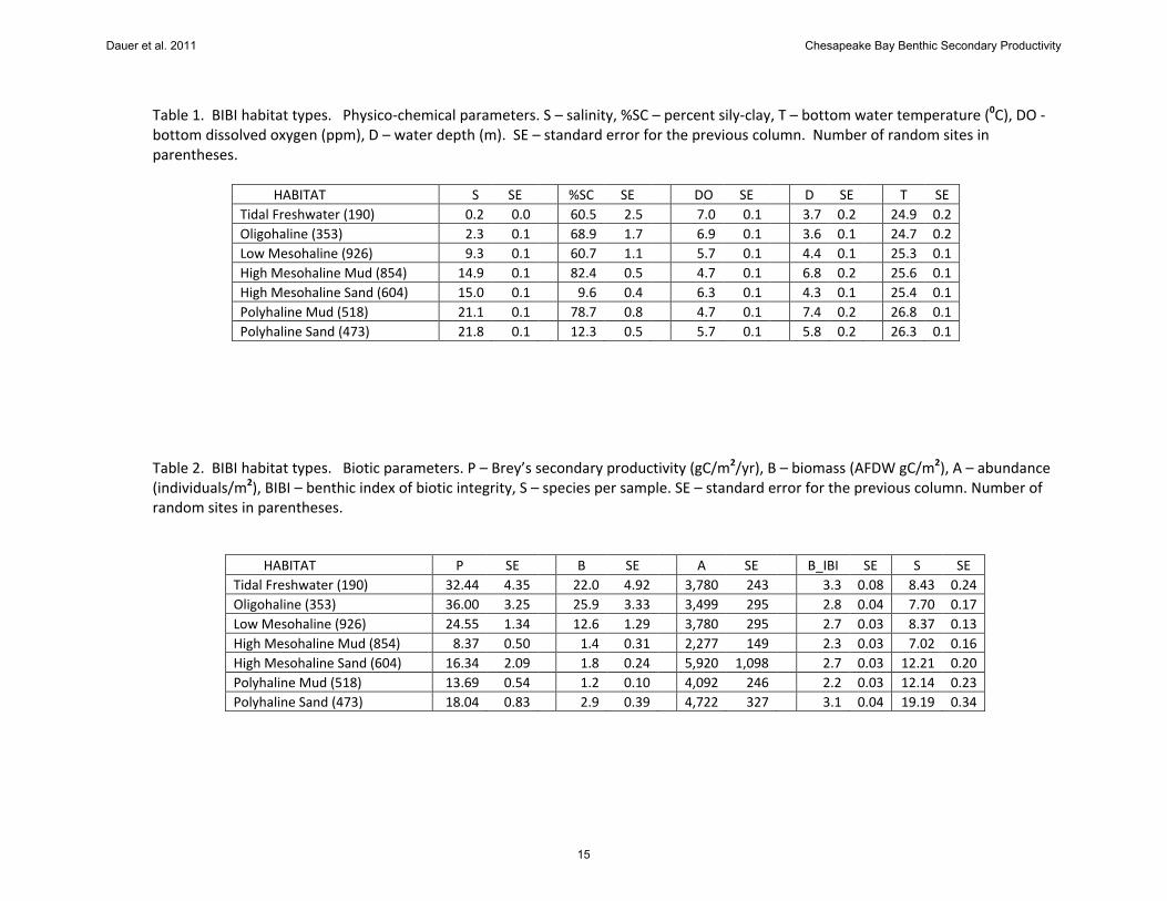
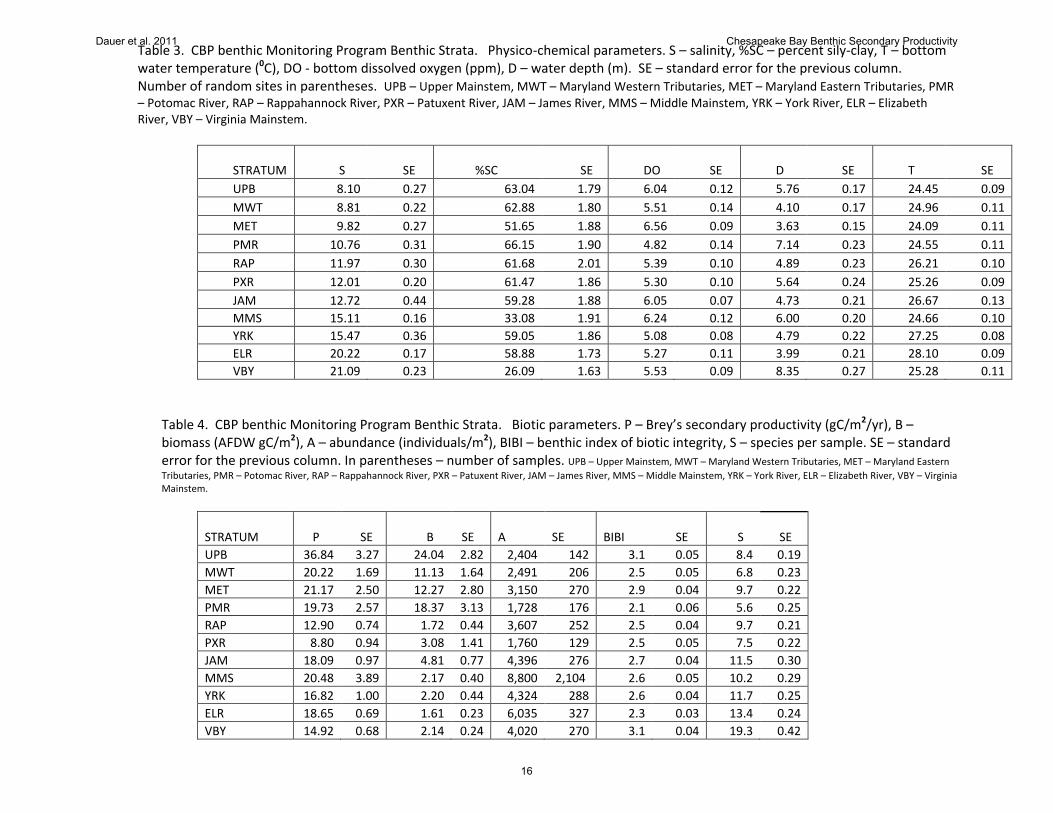
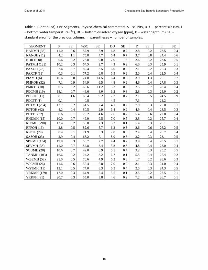
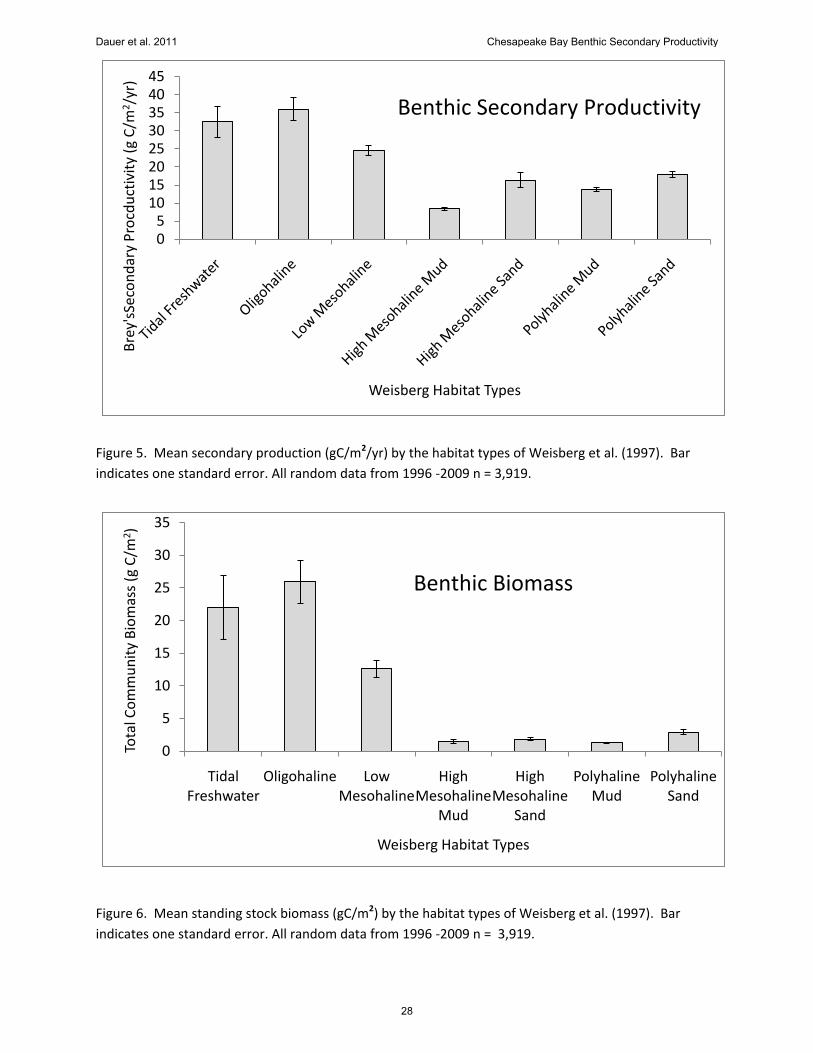
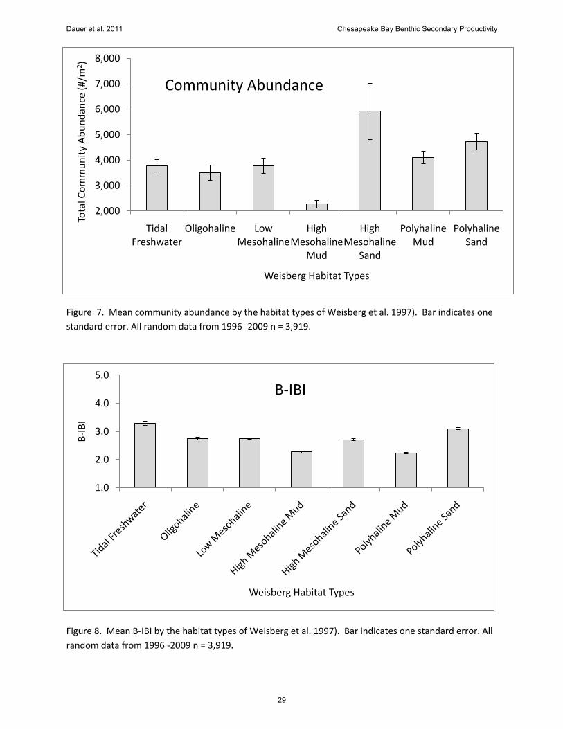
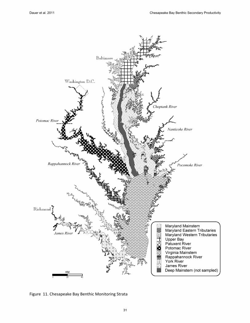
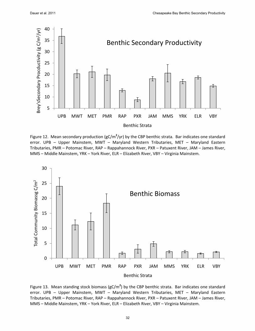
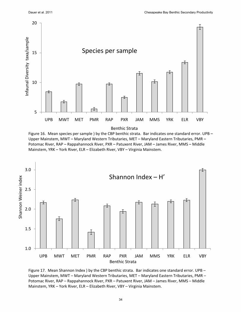
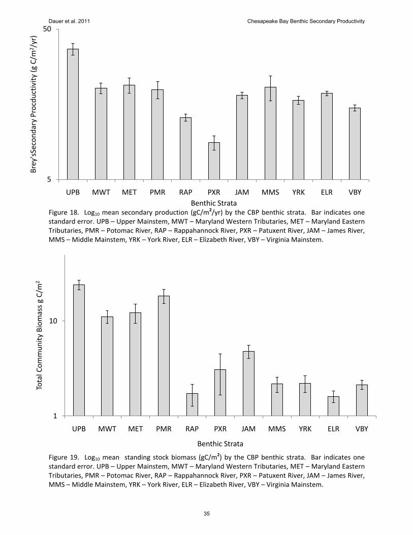
Benthic productivity - patterns and relationships with physico-chemical and benthic metrics B-IBI Habitat Types In developing the benthic index of biotic integrity, Weisberg et al. (1997) identified seven benthic habitat types in Chesapeake Bay – tidal freshwater (TF), oligohaline (OH), low mesohaline (LMH), high mesohaline mud (HMHM), high mesohaline sand (HMHS), polyhaline mud (PHM) and polyhaline sand (PHS). Benthic community metrics were selected and scored for each of these seven habitat types. For the 3,918 samples used in our study Table 1 summarizes the physico-chemical parameters and Table 2 presents Brey’s secondary productivity estimates as well as community level biomass, abundance, B-IBI values and species per sample. In Figures 5-9 the data for these benthic biotic parameters are presented as well as the Shannon Index of informational diversity in Figure 10. Both benthic secondary productivity and biomass were higher in the three lowest salinity habitat types (TF, OH, LMH)(Figures 5 and 6). This pattern is not obvious from Figure 3 were the highest benthic secondary productivity, e.g. > 200 gC/m2/yr, occurs with biomass from 10 – 700 gC/m2. These three lowest salinity habitats had the lowest species richness (Table 2 and Figure 9) and Shannon diversity (Figure 10) as expected from the general Remane Curve relationship for estuarine-transition waters but also lower abundance than the three highest salinity habitat types (HMHS, PHM,PHS) (Figure 7). CBP Benthic Monitoring Strata Since 1996 the Chesapeake Bay Benthic Monitoring Program has presented data on benthic community condition by randomly sampling all tidal waters of the Bay. Allocation of samples is random-stratified approach with each of ten strata allocated 25 random samples (sites) each year (see Figure 11 for the ten strata). The 3,918 samples used in our study were summarized by the stratum of collection. An eleventh stratum for the Elizabeth River watershed was added to the analyses in this section (ELR). The physico-chemical parameters are summarized in Table 3 and the biotic parameters in Table 4. In Figures 12-16 the data for these benthic biotic parameters are presented as well as the Shannon Index of informational diversity in Figure 17. Benthic secondary productivity varied widely with highest levels in upper mainstem of the Bay (UPB) and the lowest in the Patuxent River (PXR) (Figure 12). As such the benthic secondary productivity and biomass are plotted on a semilog scale in Figures 18 and 19, respectively. The semilog plots emphasize the disconnect in several strata between estimates of benthic secondary productivity and biomass. For example the James River had a much higher biomass than the Elizabeth River (4.81 versus 1.61 gC/m2 ) yet the Elizabeth River secondary productivity is comparable to that of the James River (18.09 gC/m2/yr in the James and 18.65 gC/m2/yr in the Elizabeth River).


6

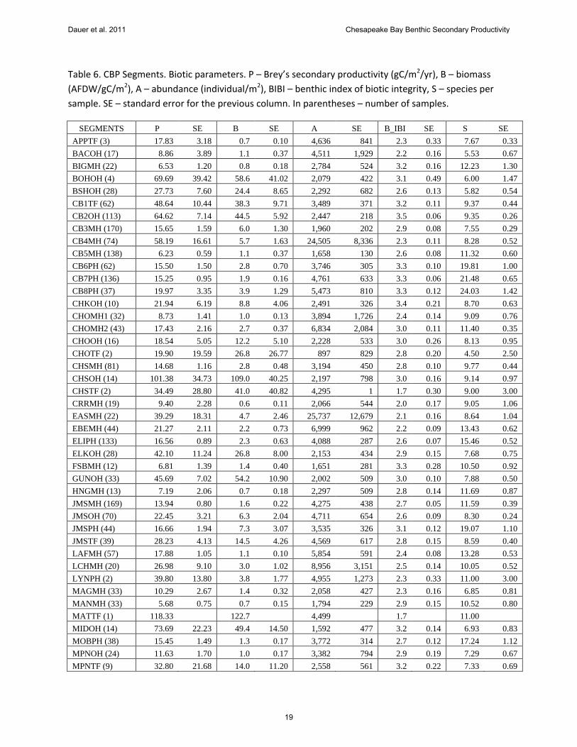
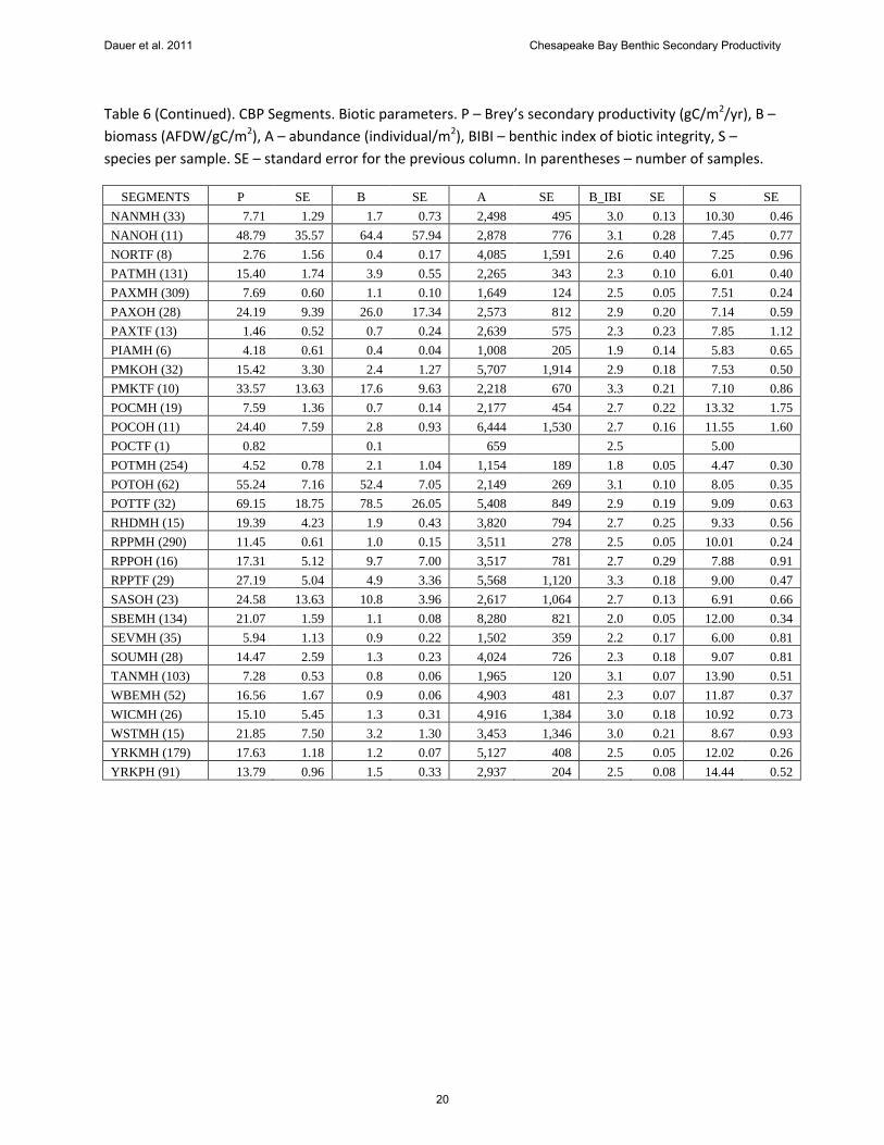
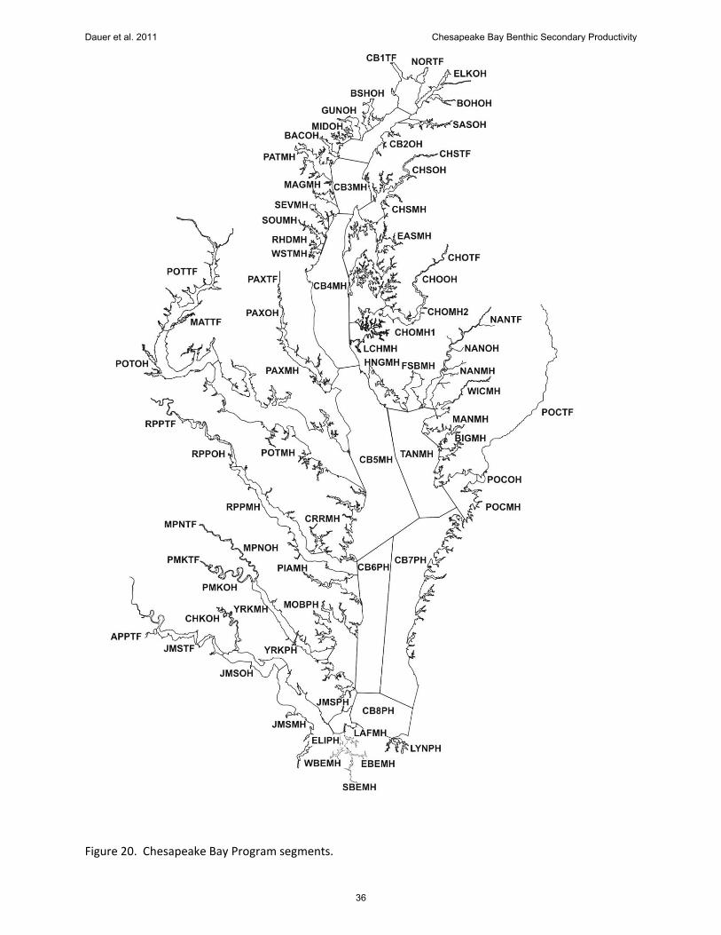
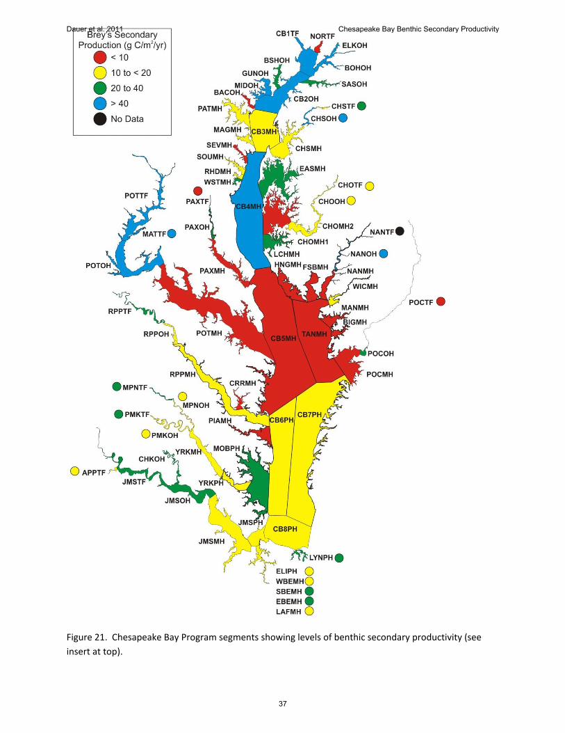
CBP monitoring Segments The Chesapeake Bay Program (CBP) divides the Bay into 73 segments (Figure 20). The 3,918 samples used in our study were summarized by CBP segments. The physico-chemical parameters are summarized in Table 5 and the biotic parameters in Table 6. The Brey’s benthic secondary productivity values for each CBP segment are summarized in Figures 21 and 22. The highest levels of benthic secondary productivity are all in Maryland and typically in TF and OH segments that have significant populations of the bivalve species Corbicula fluminea, Rangia cuneata or Gemma gemma (ELKOH, GUNOH, NANOH , POTTF, POTOH, MIDOH, CHSOH CB1TF, CB2OH and CB4MH). The second most productive segments were (1) the TF sections of the Virginia tributaries (JMSTF, PMKTF, MPNTF, RPPTF), (2) several OH sections, primarily in smaller tributaries and in Maryland (CHKOH, JMSOH, PAXOH, POCOH, SASOH, BSHOH), (3) several mesohaline small Maryland tributaries (WSTMH, LCHMH, EASMH), (4) the mouth of the Bay (CBPH8) and (5) two segments in the heavily impacted Elizabeth River watershed (SBEMH and EBEMH). The third group of segments had secondary productivity values between 10 to <20 gC/m2/yr. This group included (1) three sections of the Mainstem of the Bay bordered upstream (CB3MH) and downstream (CB6PH, CB7PH) of the Maintsem section (CB5MH) typically subjected to bottom low dissolved oxygen events, (2) all of the Rappahannock River mainstem downstream of the TF section (RPPOH, RPPMH), (3) all of the York River downstream of the TF sections, including MobJack Bay (MPNOH; PMKOH, YRKMH, YRKPH, MOBPH), (4) all of the James River mainstem downstream of the TF and OH segments (JMSMH, JMSPH), (5) most of the Choptank River (CHOMH2, CHOOH, CHOTF), (6) several mesohaline small Maryland tributaries (MAGMH, PATMH, SOUMH, CHSMH, WICMH, RHDMH), and (7) three segments in the heavily impacted Elizabeth River watershed (ELIPH, WBEMH, LAFMH). The final group of segments had secondary productivity values <10 gC/m2/yr and included (1) a single segment in the Mainstem (CB5MH), (2) numerous mesohaline segments in Maryland (POTMH, MANMH, SEVMH, BIGMH, FSBMH, HNGMH, TANMH, POCMH, PAXMH, NANMH, CHOMH1), (3) two mesohaline segments in Virginia (CRRMH, PIAMH), and (4) two lower salinity segments in Maryland (PAXTF, BACOH). CBP monitoring Segments - Low DO and Contaminant Effects The major stressors of the macrobenthic communities of Chesapeake Bay are (1) bottom low dissolved oxygen (driven primarily by excess primary production and a resulting imbalance in aerobic versus anaerobic metabolism at the ecosystem level) and (2) sediment contamination (modified by abiotic chemical and biochemical amelioration of toxic effects, as well as bioturbation effects upon bioavailability). However, in examining the patterns of benthic secondary productivity within the CBP segments two concerns were obvious – the unexpectedly high benthic secondary productivity (1) in the Mainstem segment CB4MH


7

subjected to periodic and acute low dissolved oxygen events and (2) within the CBP segments in the Elizabeth River watershed (SBEMH, EBEMH) subjected to long-term, chronic exposure to sediment contaminants, primarily high levels of PAHs (Dauer and Llanso 2003). Low Dissolved Oxygen and CBP Segment Benthic Productivity The effects on the benthos of low oxygen events are globally widespread (Diaz and Rosenberg

1995) and well documented in in Chesapeake Bay (Pihl et al., 1991; Dauer et al. 1992, 1993;

Dauer 1993). Marine and coastal ecosystems with hypoxic and or anoxic bottom water

conditions have low annual secondary production (Diaz and Rosenberg 2008). Diaz and

Rosenberg (2008) estimated for Chesapeake Bay that ~10,000 MT C is lost because of hypoxia

each year, representing ~5% of the Bay’s total secondary production. Low dissolved oxygen

events alter benthic energy flow pathways with more energy diverted into microbial pathways

including in essential benthic habitats that are nursery and recruitment areas.

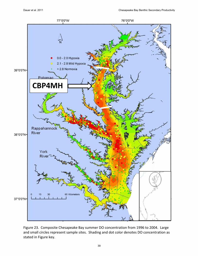
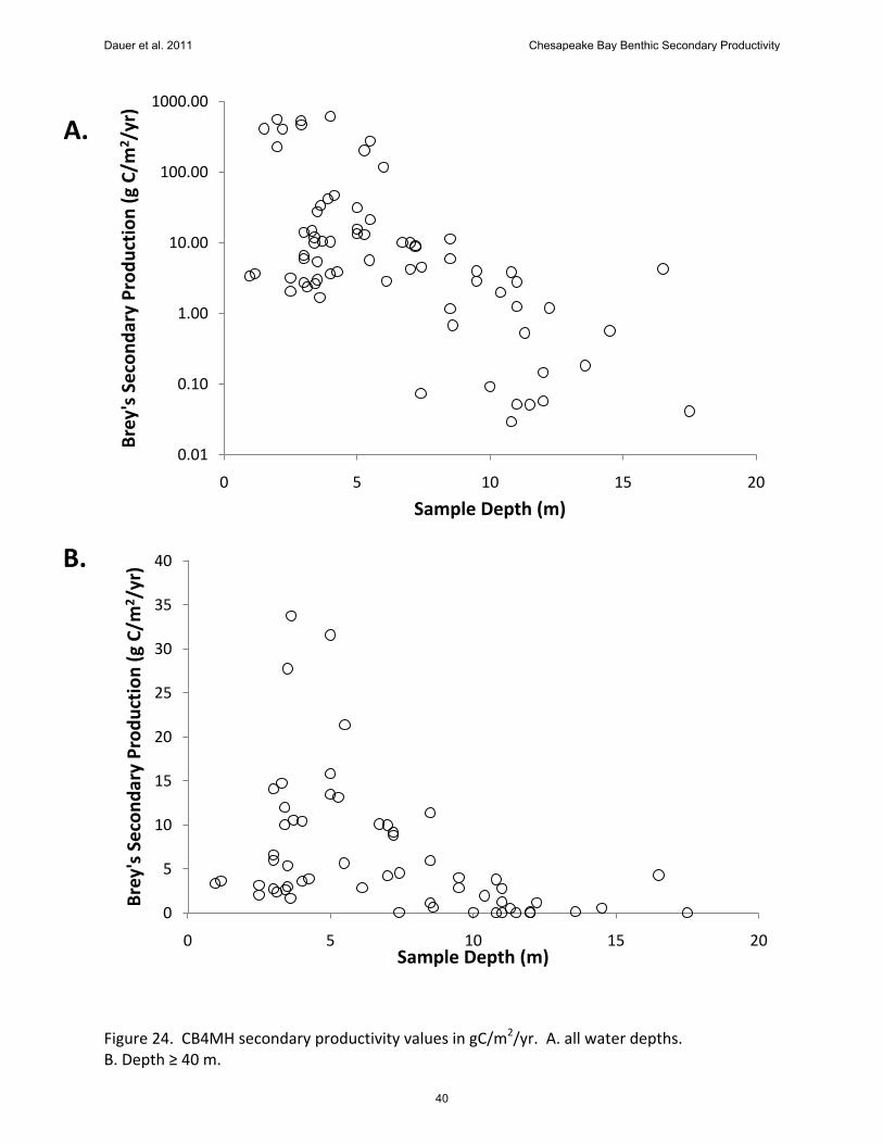
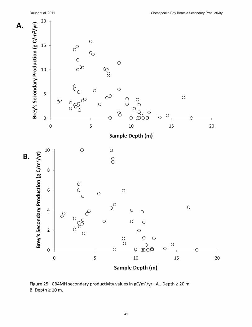
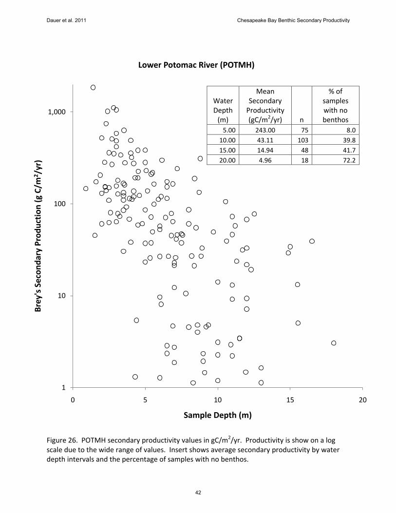
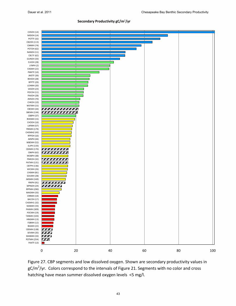
CB4MH has spatially extensive low dissolved during the summer especially in the channel region (Figure 23); however, higher dissolved oxygen levels supportive of benthos are found on the shallower shoals, particularly on the eastern side of the segment. Closer examination within CB4MH indicates that the high segment level secondary productivity values is driven by shallow water samples (<8m) highly dominated by the small but productive bivalve Gemma gemma. Figures 24 and 25 show the distribution of secondary productivity in CB4MH with various depth intervals. Lower rates of benthic production associated with lower levels of dissolved oxygen were clearly shown in other segments, for example, the lower Potomac River (POTMH). In this segment, very low bottom dissolved oxygen levels occur each summer especially at great water depths. Benthic secondary productivity was by far the highest in depths shallower than 5 m (Figure 26). Benthic secondary productivity declined from levels of 243 gC/m2/yr in water depths <5m to <5 gC/m2/yr in water depths >20m. The percentage of azoic samples (no benthos found) increased with depth with over 70% of the benthic sample in >20m being azoic. In general CBP segments with lower dissolved oxygen levels has lower benthic secondary productivity. For example, there were 12 CBP segments (excluding CBP segments with < 10 samples) with a summer mean bottom dissolved oxygen value > 5mg/l (see values in Table 5). (CBP segments with > 10 samples were excluded). These segments were (1) Mainstem segments CB3MH, CB5MH and CB6PH, (2) the lower reaches of the Potomac River (POTMH) and the York River (YRKPH), (3) the oligohaline segments of both source tributaries of the York River (MPNOH, PMKOH), and (4) several mesohaline segments in highly urbanized regions of Maryland - the Patapsco River (PATMH), the Magothy River (MAGMH), and the Severn River (SEVMH) – and Virginia’s Elizabeth River – the Southern Branch (SBEMH), and the Eastern Branch (EBEMH). Ten of the twelve segments were in the two lowest ranges of productivity (see Figure 27), except for the two segments in the Elizabeth River (the Southern Branch -SBEMH, and the Eastern Branch -EBEMH).


8

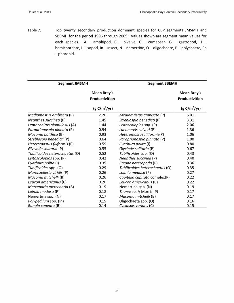
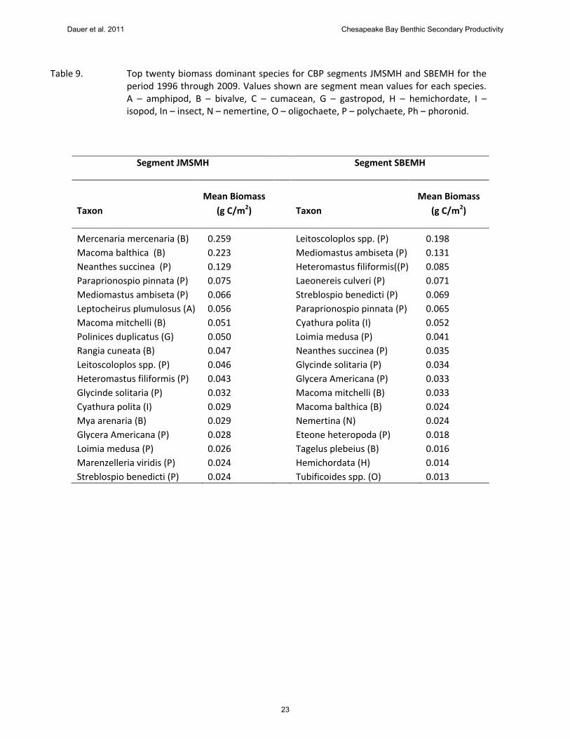
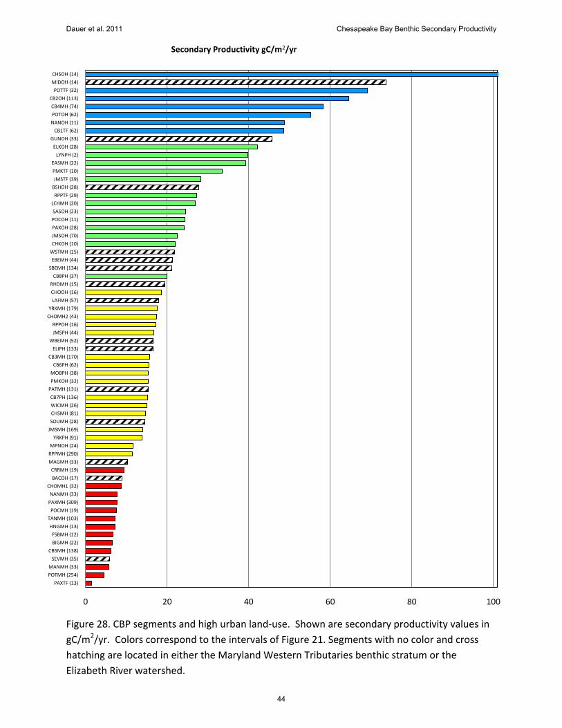
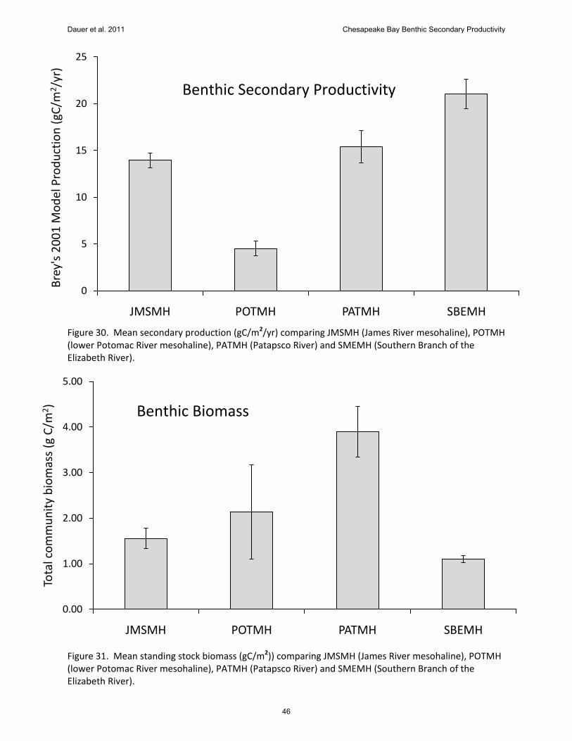
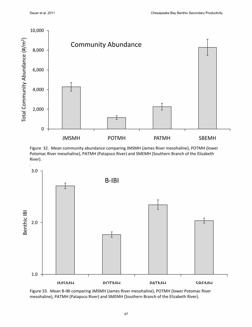
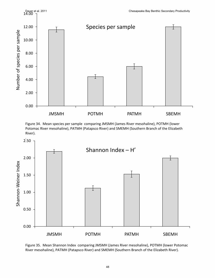
Sediment Contaminants and CBP Segment Benthic Productivity Two of the segments in the Elizabeth River were in the second highest benthic productivity level (Figure 21) although at the lower end of the scale (Figure 22). Generally sediment contaminant levels are closely related to near-field levels of urban land-use. As such Figure 22 is modified in Figures 28 and 29 to indicate the five segments of the Elizabeth River watershed (ELIPH, LAFMH, WBEMH, EBEMH, SBEMH), and the ten segments of the Maryland Western Tributaries (BSHOH, GUNOH, MIDOH, BACOH, PATMH, MAGMH, SEVMH, SOUMH, RHDMH, WSTMH) all of which are relatively small segments by benthic surface area and have shorelines with high levels of urban land-use. These small urbanized segments have values of benthic secondary productivity in all four intervals shown in Figure 21. In order to better understand the dynamics of benthic secondary production and the structural benthic metrics, four CBP segments were further compared - JMSMH, POTMH, PATMH and SBEMH. All are mesohaline regions with the James River segment (JMSMH) having no bottom low dissolved oxygen events and no known sediment contaminant levels of concern. The Potomac River segment (POTMH) has significant low dissolved oxygen events during the summer but no known sediment contaminant levels of concern. Both the Patapsco River segment (PATMH) and the Elizabeth River segment (SBEMH) are characterized by levels of sediment contaminants that have significant biological effects. The highest benthic secondary productivity (Figure 30) was in the two contaminant influenced segments (PATMH, SBEMH) a pattern not reflective of the biomass pattern (Figure 31). The lowest benthic secondary productivity value was the Potomac River which also had relatively high and variable biomass value especially compared to the James River segment (JMSMH). The two sediment contaminanted segments had similar levels of benthic secondary productivity (Figure 30) but very different biomass values (Figure 31). The high biomass values in the Patapsco River segment are driven by bivalve species Macoma balthica and Rangia cuneata that are rare in the Southern Branch of the Elizabeth River. The high levels of benthic secondary productivity in the Southern Branch is driven by the very high abundances (Figure 32) and high productivity of the polychaetes Mediomastus ambiseta and Streblospio benedicti (Tables 7- 9). B-IBI values (Figure 33), Species richness (Figure 34), and the Shannon diversity index (Figure 35) follow the expected pattern with (1) the lowest values of these three metrics in the Potomac River segment where numerous azoic samples were collected (Figure 26), (2) highest values in general at the James River segment, and (3) intermediate at the two sediment contaminated segments in the Patapsco and Elizabeth rivers. In assessing species-level influences upon benthic secondary productivity, the comparison between JMSMH and SBEMH is indicative of the disconnect between benthic community abundance (Figure 32), biomass (Figure 31) and benthic secondary productivity (Figure 30). Abundance of both segments was dominated by annelids with the top ten density dominant being annelid species in SBEMH and seven of the top ten annelids in JMSMH (Table 8). However abundances of the polychaete species Mediomastus ambiseta and Streblospio benedicti were much higher in SBEMH. Biomass dominants in SBEMH were also primarily annelids (nine of ten); however, in JMSMH the top biomass dominants included four bivalve


9

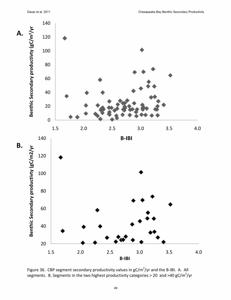
species (Mercenaria mercenaria, Macoma balthica, Macoma mitchelli, Rangia cuneata), one gastropod species (Polinices duplicatus) and one amphipod species (Leptocheirus plumulosus)(Table 9). Finally when benthic secondary productivity rates were calculated the primary differences were (1) the great importance in both segments of productivity rates of polychaete species (Mediomastus ambiseta, Streblospio benedicti, Leitoscoloplos spp., Heteromastus filiformis, Paraprionospio pinnata, Neanthes succinea), (2) the great productivity rates in JMSMH of bivalve species Macoma balthica and the amphipod Leptocheirus plumulosus that are rarely collected in SBEMH, and (3) the higher productivity rate in SBEMH of the polychaete species Laeonereis culveri that is rarely collected in JMSMH. Summary The relationship between benthic community condition as measured by the B-IBI and rates of benthic secondary productivity is not simple (Figure 36). High secondary productivity can be associated with either low BIBI levels characterized as severely degraded (BIBI ≤ 2.0) or with BIBI values considered undegraded (BIBI ≥ 3.0). In addition, regions with high levels of sediment contaminants such as the Patapsco River and Elizabeth River can have unexpectedly high levels of benthic secondary productivity The next steps in using benthic secondary productivity estimates is to develop a protocol to reflect the actual availability of the benthic production to higher trophic levels. Important ecological factors are (1) protective coverings such has molluscan shells and crustacean exoskeletons that reduce predation, (2) depth of dwelling within the sediment that might provide a refuge from predation, (3) body size factors that affect strength of protective coverings and/or age-related sediment depth dwelling location, and (4) general behaviors that can modify susceptibility to predation, e.g. rapid motility. In natural ecosystems, local species diversity and productivity are regulated by a myriad of interacting factors at a variety of temporal and spatial scales. Ecological status assessment is essential to direct maintenance, protection, and/or restoration efforts in regard to marine and estuarine ecosystem services. Parameters that assess ecosystem structure are widely used, diverse, and often profligate. Parameters that assess ecosystem function should be less variable and better understood in directing ecosystem management decisions. Thus assessment of benthic secondary productivity estimates as a management assessment tool deserves serious further consideration, development as a tool and application in management decisions.


10

Literature Cited Alden, R.W. III, S.B. Weisberg, J.A. Ranasinghe, and D.M. Dauer. 1997. Optimizing temporal sampling strategies for benthic environmental monitoring programs. Marine Pollution Bulletin 34:913-922. Asmus, H., 1987. Secondary production of an intertidal mussel bed community related to its storage and turnover compartments. Marine Ecology Progress Series. 39:251-266. Bilyard, G.R., 1987. The value of benthic infauna in marine pollution monitoring studies. Marine Pollution Bulletin. 18:581-585. Boesch, D.F., 1973. Classification and community structure of the macrobenthos in the Hampton Roads area, Virginia. Marine Biology. 21:226-224. Boesch, D.F. 1977. A new look at zonation of the benthos along the estuarine gradient. pp. 285-308, In Marine Benthic Dynamic, K.R. Tenore and B.C. Coull, eds., University of South Carolina Press, Columbia SC. Bolam, S.G., J. Barry, T. Bolam, C. Mason, H.S. Rumney, J.E. Thain, and R.J. Law. 2011. Impacts of maintenance dredged material disposal on macrobenthic structure and secondary productivity. Marine Pollution Bulletin 62:2230-2245. Borja, A. and D.M. Dauer. 2008. Assessing the environmental quality status in estuarine and coastal systems: comparing methodologies and indices. Ecological Indicators 8: 331-337. Borja, A, S.B. Bricker, D.M. Dauer, N.T. Demetriades, J.G. Ferreira, A. T. Forbes, P. Hutchings, X. Jia, R.Kenchington, J.C. Marques and C. Zhu. 2008. Overview of integrative tools and methods in assessing ecological integrity in estuarine and coastal systems worldwide. Marine Pollution Bulletin 56: 1519-1537.

Borja, A, D.M. Dauer, M. Elliott, and C.A. Simenstad. 2010. Medium and long-term recovery of estuarine and coastal ecosystems: patterns, rates and restoration effectiveness. Estuaries and Coasts 33:1249–1260. Borja, Á, D. M. Dauer, and A. Grémare. 2011. The importance of setting targets and reference conditions in assessing marine ecosystem quality. Ecological Indicators. 12:1-7. Brey, T. 1999. A collection of empirical relations for use in ecological modelling. ICLARM Quarterly 22:24-28. Brey, T. 2001. Population dynamics in benthic invertebrates. A virtual handbook. Version 01.2. http://www.thomas-brey.de/science/virtualhandbook.


11

http://www.thomas-brey.de/science/virtualhandbook.

Cusson, M. and E. Bourget, 2005. Global patterns of macroinvertebrate production in marine benthic habitats. Marine Ecology Progress Series. 279:1-14. Dauer, D.M., 1993. Biological criteria, environmental health and estuarine macrobenthic community structure. Marine Pollution Bulletin 26: 249-257. Dauer, D.M. 1997. Dynamics of an estuarine ecosystem: Long-term trends in the macrobenthic communities of the Chesapeake Bay, USA (1985-1993). Oceanologica Acta 20:291-298. Dauer, D.M. 2000. Benthic Biological Monitoring Program of the Elizabeth River Watershed (1999). Final Report to the Virginia Department of Environmental Quality, Chesapeake Bay Program, 73 pp. Dauer, D.M. 2009. Benthic Biological Monitoring Program of the Elizabeth River Watershed (2008). Final Report to the Virginia Department of Environmental Quality, Chesapeake Bay Program, 119 pp. Dauer, D.M. and R.W. Alden III. 1995. Long-term trends in the macrobenthic communities of the lower Chesapeake Bay (1985-1991). Marine Pollution Bulletin 30:840-850. Dauer, D.M. and R.J. Llansó. 2003. Spatial scales and probability based sampling in determining levels of benthic community degradation in the Chesapeake Bay. Environmental Monitoring and Assessment 81:175-186. Dauer, D.M., Luckenbach. M.W. and A.J. Rodi, Jr. 1993. Abundance biomass comparison (ABC method): effects of an estuarine gradient, anoxic/hypoxic events and contaminated sediments. Marine Biology 116: 507-518. Dauer, D.M., J. A. Ranasinghe, and S. B. Weisberg. 2000. Relationships between benthic Community condition, water quality, sediment quality, nutrient loads, and land use patterns in Chesapeake Bay. Estuaries 23: 80-96. Dauer, D.M., Rodi, A.J., Ranasinghe, J.A., 1992. Effects of low dissolved oxygen events on the macrobenthos of the lower Chesapeake Bay. Estuaries 15, 384– 391. Diaz, R.J. and R. Rosenberg, R., 1995. Marine benthic hypoxia: a review of its ecological effects and the behavioural responses of benthic macrofauna. Annual Review of Oceanography and Marine Biology 33: 245– 303.

Diaz, R.J. and R. Rosenberg, R., 2008. Spreading dead zones and consequences for marine

ecosystems. Science 32: 926-929


12

Diaz, R.J. and L.C. Schaffner. 1990. pp. 25–56, in Perspectives in the Chesapeake Bay: Advances

in Estuarine Sciences, M. Haire, E. C. Krome, Eds., Chesapeake Research Consortium,

Gloucester Point, VA.

Dolbeth, M., A.I. Lillebø, P.G. Cardoso, S.M. Ferreira, and M.A. Pardal, 2005. Annual production of estuarine fauna in different environmental conditions: An evaluation of the estimation methods. Journal of Experimental Marine Biology and Ecology 326:115-127. Dolbeth, M., M. A. Pardal, A. I. Lillebø, U. Azeiteiro, and J. C. Marques, 2003. Short- and long-term effects of eutrophication on the secondary production of an intertidal macrobenthic community. Marine Biology. 143:1229-1238 Edgar, G.J., 1990. The use of the size structure of benthic macrofaunal communities to estimate faunal biomass and secondary production. Journal of Experimental Marine Biology and Ecology 137:195-214. Flint, R.W., 1985. Long-term estuarine variability and associated biological response. Estuaries 8:158-189. Gillet, D.J. 2010. Effects of habitat quality on secondary production in shallow estuarine waters and the consequences for the benthic-pelagic food web. PhD Dissertation. College of William and Mary, Virginia. 175 p. Gray, J. S., M. Ascan, M.R. Carr, K.R. Clarke, R.H. Green, T.H. Pearson, R. Rosenberg, and R.W. Warwick, 1988. Analysis of community attributes of the benthic macrofauna of Frierfjord/ Langesundfjord and in a mesocosm experiment. Marine Ecology Progress Series 46:151-165. Holland, A. E, Mountford, N. K., Hiegel, M. H., Kaumeyer, K. R. and Mihursky, J. A. (1980). Influence of predation on infaunal abundance in upper Chesapeake Bay. Marine Biology 57:221-235. Llansó, R.J., D.M. Dauer, and J.H. Vølstad. 2009. Assessing ecological integrity for impaired waters decisions in Chesapeake Bay, USA. Marine Pollution Bulletin 59: 48-53. Llansó, R.J., D.M. Dauer, J.H. Vølstad, and L.S. Scott. 2003. Application of the Benthic Index of Biotic Integrity to environmental monitoring in Chesapeake Bay. Environmental Monitoring and Assessment 81:163-174. Nixon, S.W. and B.A. Buckley, 2002. "A strikingly rich zone" Nutrient enrichment and secondary production in coastal marine ecosystems. Estuaries 25:782-796. Pearson, T., and R. Rosenberg, 1978. Macrobenthic succession in relation to organic enrichment and pollution of the marine environment. Oceanography Marine Biology Annual Review. 16:229-311.


13

Pihl, L., S. P. Baden, and R. J. Diaz. 1991. Effects of periodic hypoxia on distribution of demersal fish and crustaceans. Marine Biology 108:349-360. Reisch, D., 1973. The use of benthic animals in monitoring the marine environment. Journal of Environmental Planning and Pollution Control. 1:32:38. Schwinghamer, P., B. Hargrave, D. Peer, C.M. Hawkins, 1986. Partitioning of production and respiration among size groups of organisms in an intertidal benthic community. Marine Ecology Progress Series 31:131-142. Steimle, F.W. Jr., 1985. Biomass and estimated productivity of the benthic macrofauna in the New York Bight: a stressed coastal area. Estuarine, Coastal and Shelf Science 21:539-554. Sturdivant, S.K., 2011. The effects of hypoxia on macrobenthic production and function in the lower Rappahannock River, Chesapeake Bay, USA. PhD. Dissertation. College of William and Mary, Virginia. Tumbiolo, M.L. and J. Downing, 1994. An empirical model for the prediction of secondary production in marine benthic invertebrate populations. Marine Ecology Progress Series 114:165-174. Wilber, D.H. and D.G. Clarke, 1998. Estimating secondary production and benthic consumption in monitoring studies: a case study of impacts of dredged material disposal in Galveston Bay. Estuaries. 21:230-245. Wilson, J.G., 2002. Productivity, fisheries and aquaculture in temperate estuaries. Estuarine, Coastal and Shelf Science. 55:953-967.


14

Table 1. BIBI habitat types. Physico-chemical parameters. S – salinity, %SC – percent sily-clay, T – bottom water temperature (0C), DO - bottom dissolved oxygen (ppm), D – water depth (m). SE – standard error for the previous column. Number of random sites in parentheses.

HABITAT S SE %SC SE DO SE D SE T SE

Tidal Freshwater (190) 0.2 0.0 60.5 2.5 7.0 0.1 3.7 0.2 24.9 0.2

Oligohaline (353) 2.3 0.1 68.9 1.7 6.9 0.1 3.6 0.1 24.7 0.2

Low Mesohaline (926) 9.3 0.1 60.7 1.1 5.7 0.1 4.4 0.1 25.3 0.1

High Mesohaline Mud (854) 14.9 0.1 82.4 0.5 4.7 0.1 6.8 0.2 25.6 0.1

High Mesohaline Sand (604) 15.0 0.1 9.6 0.4 6.3 0.1 4.3 0.1 25.4 0.1

Polyhaline Mud (518) 21.1 0.1 78.7 0.8 4.7 0.1 7.4 0.2 26.8 0.1

Polyhaline Sand (473) 21.8 0.1 12.3 0.5 5.7 0.1 5.8 0.2 26.3 0.1

Table 2. BIBI habitat types. Biotic parameters. P – Brey’s secondary productivity (gC/m2/yr), B – biomass (AFDW gC/m2), A – abundance (individuals/m2), BIBI – benthic index of biotic integrity, S – species per sample. SE – standard error for the previous column. Number of random sites in parentheses.

HABITAT P SE B SE A SE B_IBI SE S SE

Tidal Freshwater (190) 32.44 4.35 22.0 4.92 3,780 243 3.3 0.08 8.43 0.24

Oligohaline (353) 36.00 3.25 25.9 3.33 3,499 295 2.8 0.04 7.70 0.17

Low Mesohaline (926) 24.55 1.34 12.6 1.29 3,780 295 2.7 0.03 8.37 0.13

High Mesohaline Mud (854) 8.37 0.50 1.4 0.31 2,277 149 2.3 0.03 7.02 0.16

High Mesohaline Sand (604) 16.34 2.09 1.8 0.24 5,920 1,098 2.7 0.03 12.21 0.20

Polyhaline Mud (518) 13.69 0.54 1.2 0.10 4,092 246 2.2 0.03 12.14 0.23

Polyhaline Sand (473) 18.04 0.83 2.9 0.39 4,722 327 3.1 0.04 19.19 0.34


15

Table 3. CBP benthic Monitoring Program Benthic Strata. Physico-chemical parameters. S – salinity, %SC – percent sily-clay, T – bottom water temperature (0C), DO - bottom dissolved oxygen (ppm), D – water depth (m). SE – standard error for the previous column. Number of random sites in parentheses. UPB – Upper Mainstem, MWT – Maryland Western Tributaries, MET – Maryland Eastern Tributaries, PMR – Potomac River, RAP – Rappahannock River, PXR – Patuxent River, JAM – James River, MMS – Middle Mainstem, YRK – York River, ELR – Elizabeth River, VBY – Virginia Mainstem.

STRATUM S SE %SC SE DO SE D SE T SE

UPB 8.10 0.27 63.04 1.79 6.04 0.12 5.76 0.17 24.45 0.09

MWT 8.81 0.22 62.88 1.80 5.51 0.14 4.10 0.17 24.96 0.11

MET 9.82 0.27 51.65 1.88 6.56 0.09 3.63 0.15 24.09 0.11

PMR 10.76 0.31 66.15 1.90 4.82 0.14 7.14 0.23 24.55 0.11

RAP 11.97 0.30 61.68 2.01 5.39 0.10 4.89 0.23 26.21 0.10

PXR 12.01 0.20 61.47 1.86 5.30 0.10 5.64 0.24 25.26 0.09

JAM 12.72 0.44 59.28 1.88 6.05 0.07 4.73 0.21 26.67 0.13

MMS 15.11 0.16 33.08 1.91 6.24 0.12 6.00 0.20 24.66 0.10

YRK 15.47 0.36 59.05 1.86 5.08 0.08 4.79 0.22 27.25 0.08

ELR 20.22 0.17 58.88 1.73 5.27 0.11 3.99 0.21 28.10 0.09

VBY 21.09 0.23 26.09 1.63 5.53 0.09 8.35 0.27 25.28 0.11

Table 4. CBP benthic Monitoring Program Benthic Strata. Biotic parameters. P – Brey’s secondary productivity (gC/m2/yr), B – biomass (AFDW gC/m2), A – abundance (individuals/m2), BIBI – benthic index of biotic integrity, S – species per sample. SE – standard error for the previous column. In parentheses – number of samples. UPB – Upper Mainstem, MWT – Maryland Western Tributaries, MET – Maryland Eastern

Tributaries, PMR – Potomac River, RAP – Rappahannock River, PXR – Patuxent River, JAM – James River, MMS – Middle Mainstem, YRK – York River, ELR – Elizabeth River, VBY – Virginia Mainstem.

STRATUM P SE B SE A SE BIBI SE S SE

UPB 36.84 3.27 24.04 2.82 2,404 142 3.1 0.05 8.4 0.19

MWT 20.22 1.69 11.13 1.64 2,491 206 2.5 0.05 6.8 0.23

MET 21.17 2.50 12.27 2.80 3,150 270 2.9 0.04 9.7 0.22

PMR 19.73 2.57 18.37 3.13 1,728 176 2.1 0.06 5.6 0.25

RAP 12.90 0.74 1.72 0.44 3,607 252 2.5 0.04 9.7 0.21

PXR 8.80 0.94 3.08 1.41 1,760 129 2.5 0.05 7.5 0.22

JAM 18.09 0.97 4.81 0.77 4,396 276 2.7 0.04 11.5 0.30

MMS 20.48 3.89 2.17 0.40 8,800 2,104 2.6 0.05 10.2 0.29

YRK 16.82 1.00 2.20 0.44 4,324 288 2.6 0.04 11.7 0.25

ELR 18.65 0.69 1.61 0.23 6,035 327 2.3 0.03 13.4 0.24

VBY 14.92 0.68 2.14 0.24 4,020 270 3.1 0.04 19.3 0.42


16

Table 5. CBP Segments. Physico-chemical parameters. S – salinity, %SC – percent silt-clay, T – bottom

water temperature (0C), DO – bottom dissolved oxygen (ppm), D – water depth (m). SE – standard error

for the previous column. In parentheses – number of samples.

SEGMENT S SE %SC SE DO SE D SE T SE

APPTF (3) 0.1 0.0 59.8 9.8 6.6 0.4 4.4 1.1 28.8 1.2

BACOH (17) 3.1 0.6 66.8 8.5 8.4 0.7 1.6 0.2 25.1 0.5

BIGMH (22) 16.6 0.4 39.4 6.8 7.1 0.2 2.4 0.2 24.4 0.6

BOHOH (4) 5.3 1.9 65.3 17.5 8.0 0.2 2.1 0.3 24.7 1.2

BSHOH (28) 3.4 0.4 83.8 3.2 8.4 0.3 2.1 0.1 22.1 0.4

CB1TF (62) 1.1 0.2 40.2 3.8 8.1 0.2 3.3 0.3 23.5 0.3

CB2OH (113) 7.0 0.3 69.6 2.7 6.8 0.1 5.3 0.2 24.4 0.2

CB3MH (170) 11.8 0.2 66.0 2.7 4.8 0.2 7.0 0.2 24.9 0.1

CB4MH (74) 14.1 0.4 38.0 4.5 6.0 0.3 6.6 0.5 24.6 0.2

CB5MH (138) 17.0 0.2 23.4 2.7 4.8 0.2 9.8 0.4 25.4 0.2

CB6PH (62) 20.8 0.5 36.4 4.4 4.9 0.2 9.2 0.3 25.1 0.2

CB7PH (136) 22.8 0.3 21.0 2.2 5.6 0.1 9.2 0.4 24.9 0.2

CB8PH (37) 24.8 0.5 12.6 2.2 6.0 0.1 8.0 0.4 24.1 0.4

CHKOH (10) 1.5 0.6 69.1 9.1 6.7 0.4 2.0 0.3 28.7 0.5

CHOMH1 (32) 13.3 0.4 46.5 6.5 6.9 0.4 5.0 0.6 24.2 0.4

CHOMH2 (43) 10.7 0.3 48.7 5.2 6.4 0.1 4.4 0.4 23.9 0.3

CHOOH (16) 4.6 0.8 57.1 8.0 5.8 0.4 5.3 0.8 23.2 0.3

CHOTF (2) 0.8 0.1 92.9 0.9 7.2 1.1 2.9 0.1 24.7 3.0

CHSMH (81) 11.7 0.2 38.5 4.0 5.5 0.2 4.9 0.4 24.5 0.2

CHSOH (14) 6.8 0.9 74.3 6.0 6.0 0.4 3.0 0.5 24.4 0.5

CHSTF (2) 3.0 2.4 92.6 1.7 5.2 0.3 1.7 0.3 22.9 2.1

CRRMH (19) 15.6 0.4 53.8 9.8 5.1 0.3 3.2 0.5 27.4 0.5

EASMH (22) 13.4 0.4 35.8 7.8 7.0 0.3 3.8 0.6 23.8 0.3

EBEMH (44) 17.5 0.6 70.4 4.3 4.5 0.3 3.3 0.4 27.6 0.2

ELIPH (133) 21.5 0.2 51.8 3.2 5.4 0.1 6.5 0.5 27.3 0.1

ELKOH (28) 2.7 0.3 60.3 6.6 7.1 0.3 3.5 0.7 23.9 0.4

FSBMH (12) 11.8 1.1 70.0 8.3 7.2 0.4 2.3 0.2 21.0 1.0

GUNOH (33) 4.5 0.5 70.7 5.8 7.3 0.2 2.2 0.2 22.9 0.4

HNGMH (13) 15.1 0.6 37.0 7.9 7.3 0.2 2.9 0.4 25.2 0.5

JMSMH (169) 15.9 0.4 58.4 2.6 6.1 0.1 4.1 0.2 26.3 0.2

JMSOH (70) 5.8 0.5 64.6 4.7 6.3 0.2 3.8 0.3 27.8 0.2

JMSPH (44) 22.5 0.4 39.2 5.1 5.8 0.1 8.3 0.8 25.4 0.3

JMSTF (39) 0.6 0.1 71.4 5.3 6.4 0.2 4.8 0.7 26.6 0.4

LAFMH (57) 19.3 0.4 69.8 4.3 6.6 0.3 1.9 0.2 28.9 0.2

LCHMH (20) 14.9 0.4 30.3 7.8 7.9 0.3 2.6 0.5 23.7 0.4

LYNPH (2) 19.8 0.8 61.3 12.3 3.2 2.9 1.3 0.7 28.3 0.3

MAGMH (33) 11.1 0.6 53.7 6.7 4.6 0.4 3.8 0.4 24.9 0.3

MANMH (33) 15.6 0.3 41.3 6.2 7.3 0.2 2.3 0.2 25.0 0.3

MATTF (1) 2.1 16.7 6.5 2.7 25.4

MIDOH (14) 4.4 0.6 58.9 10.5 7.6 0.2 2.1 0.2 25.3 0.5

MOBPH (38) 19.6 0.6 37.4 5.8 5.7 0.3 5.3 0.7 26.4 0.2

MPNOH (24) 6.9 1.3 48.7 8.1 4.1 0.2 6.0 0.7 27.6 0.3

MPNTF (9) 0.3 0.2 29.8 12.7 5.2 0.2 3.7 0.8 25.3 0.5


17

Table 5. (Continued). CBP Segments. Physico-chemical parameters. S – salinity, %SC – percent silt-clay, T

– bottom water temperature (0C), DO – bottom dissolved oxygen (ppm), D – water depth (m). SE –

standard error for the previous column. In parentheses – number of samples.

SEGMENT S SE %SC SE DO SE D SE T SE

NANMH (33) 11.0 0.6 57.9 5.9 6.8 0.2 2.8 0.2 23.5 0.4

NANOH (11) 4.2 1.1 75.8 4.7 6.4 0.7 3.7 0.8 24.4 0.6

NORTF (8) 0.6 0.2 73.8 9.0 7.0 1.3 2.6 0.2 23.6 0.5

PATMH (131) 10.2 0.3 64.5 2.7 4.3 0.2 6.0 0.3 25.9 0.1

PAXOH (28) 7.4 0.7 82.4 3.5 6.0 0.3 2.1 0.2 25.3 0.3

PAXTF (13) 0.3 0.1 77.2 6.8 6.3 0.2 2.0 0.4 22.5 0.4

PIAMH (6) 16.6 0.8 74.0 14.5 6.4 0.6 3.9 1.3 25.1 0.7

PMKOH (32) 7.1 0.9 54.9 6.5 4.8 0.2 4.6 0.4 27.8 0.3

PMKTF (10) 0.5 0.2 68.6 11.2 5.3 0.5 2.5 0.7 28.4 0.4

POCMH (19) 18.1 0.7 46.6 8.0 6.2 0.3 2.8 0.3 25.0 0.2

POCOH (11) 8.1 1.6 65.4 9.2 7.2 0.7 2.1 0.5 24.5 0.9

POCTF (1) 0.1 0.8 4.5 7.3 21.2

POTMH (254) 13.7 0.2 61.5 2.4 4.1 0.2 7.9 0.3 25.0 0.1

POTOH (62) 4.2 0.4 80.5 2.9 6.4 0.2 4.9 0.4 23.5 0.3

POTTF (32) 0.6 0.1 79.2 4.6 7.6 0.2 5.4 0.6 22.8 0.4

RHDMH (15) 10.0 0.7 49.9 9.5 7.0 0.5 2.8 0.2 25.7 0.4

RPPMH (290) 13.4 0.2 59.8 2.3 5.2 0.1 5.4 0.3 26.1 0.1

RPPOH (16) 2.8 0.5 82.6 5.7 6.2 0.3 2.6 0.6 26.2 0.5

RPPTF (29) 0.4 0.1 71.9 5.3 7.0 0.3 2.4 0.4 26.7 0.4

SASOH (23) 2.9 0.4 66.2 7.1 8.0 0.3 3.2 0.3 23.1 0.5

SBEMH (134) 19.9 0.3 53.7 2.7 4.4 0.2 3.9 0.4 28.5 0.1

SEVMH (35) 11.0 0.7 57.8 5.4 3.8 0.5 4.8 0.4 25.0 0.4

SOUMH (28) 10.6 0.7 42.0 6.9 5.1 0.4 3.2 0.3 25.2 0.5

TANMH (103) 16.6 0.2 24.2 3.2 6.7 0.1 5.5 0.4 25.4 0.2

WBEMH (52) 21.0 0.5 70.6 4.9 6.2 0.3 1.7 0.2 28.6 0.3

WICMH (26) 11.6 0.6 52.4 6.8 7.0 0.2 3.1 0.3 24.0 0.4

WSTMH (15) 12.1 0.5 74.0 8.3 6.3 0.4 2.5 0.3 24.3 0.5

YRKMH (179) 17.0 0.3 64.9 2.4 5.5 0.1 3.5 0.2 27.5 0.1

YRKPH (91) 20.7 0.3 55.0 3.8 4.6 0.2 7.2 0.6 26.7 0.1


18

Table 6. CBP Segments. Biotic parameters. P – Brey’s secondary productivity (gC/m2/yr), B – biomass

(AFDW/gC/m2), A – abundance (individual/m2), BIBI – benthic index of biotic integrity, S – species per

sample. SE – standard error for the previous column. In parentheses – number of samples.

SEGMENTS P SE B SE A SE B_IBI SE S SE

APPTF (3) 17.83 3.18 0.7 0.10 4,636 841 2.3 0.33 7.67 0.33

BACOH (17) 8.86 3.89 1.1 0.37 4,511 1,929 2.2 0.16 5.53 0.67

BIGMH (22) 6.53 1.20 0.8 0.18 2,784 524 3.2 0.16 12.23 1.30

BOHOH (4) 69.69 39.42 58.6 41.02 2,079 422 3.1 0.49 6.00 1.47

BSHOH (28) 27.73 7.60 24.4 8.65 2,292 682 2.6 0.13 5.82 0.54

CB1TF (62) 48.64 10.44 38.3 9.71 3,489 371 3.2 0.11 9.37 0.44

CB2OH (113) 64.62 7.14 44.5 5.92 2,447 218 3.5 0.06 9.35 0.26

CB3MH (170) 15.65 1.59 6.0 1.30 1,960 202 2.9 0.08 7.55 0.29

CB4MH (74) 58.19 16.61 5.7 1.63 24,505 8,336 2.3 0.11 8.28 0.52

CB5MH (138) 6.23 0.59 1.1 0.37 1,658 130 2.6 0.08 11.32 0.60

CB6PH (62) 15.50 1.50 2.8 0.70 3,746 305 3.3 0.10 19.81 1.00

CB7PH (136) 15.25 0.95 1.9 0.16 4,761 633 3.3 0.06 21.48 0.65

CB8PH (37) 19.97 3.35 3.9 1.29 5,473 810 3.3 0.12 24.03 1.42

CHKOH (10) 21.94 6.19 8.8 4.06 2,491 326 3.4 0.21 8.70 0.63

CHOMH1 (32) 8.73 1.41 1.0 0.13 3,894 1,726 2.4 0.14 9.09 0.76

CHOMH2 (43) 17.43 2.16 2.7 0.37 6,834 2,084 3.0 0.11 11.40 0.35

CHOOH (16) 18.54 5.05 12.2 5.10 2,228 533 3.0 0.26 8.13 0.95

CHOTF (2) 19.90 19.59 26.8 26.77 897 829 2.8 0.20 4.50 2.50

CHSMH (81) 14.68 1.16 2.8 0.48 3,194 450 2.8 0.10 9.77 0.44

CHSOH (14) 101.38 34.73 109.0 40.25 2,197 798 3.0 0.16 9.14 0.97

CHSTF (2) 34.49 28.80 41.0 40.82 4,295 1 1.7 0.30 9.00 3.00

CRRMH (19) 9.40 2.28 0.6 0.11 2,066 544 2.0 0.17 9.05 1.06

EASMH (22) 39.29 18.31 4.7 2.46 25,737 12,679 2.1 0.16 8.64 1.04

EBEMH (44) 21.27 2.11 2.2 0.73 6,999 962 2.2 0.09 13.43 0.62

ELIPH (133) 16.56 0.89 2.3 0.63 4,088 287 2.6 0.07 15.46 0.52

ELKOH (28) 42.10 11.24 26.8 8.00 2,153 434 2.9 0.15 7.68 0.75

FSBMH (12) 6.81 1.39 1.4 0.40 1,651 281 3.3 0.28 10.50 0.92

GUNOH (33) 45.69 7.02 54.2 10.90 2,002 509 3.0 0.10 7.88 0.50

HNGMH (13) 7.19 2.06 0.7 0.18 2,297 509 2.8 0.14 11.69 0.87

JMSMH (169) 13.94 0.80 1.6 0.22 4,275 438 2.7 0.05 11.59 0.39

JMSOH (70) 22.45 3.21 6.3 2.04 4,711 654 2.6 0.09 8.30 0.24

JMSPH (44) 16.66 1.94 7.3 3.07 3,535 326 3.1 0.12 19.07 1.10

JMSTF (39) 28.23 4.13 14.5 4.26 4,569 617 2.8 0.15 8.59 0.40

LAFMH (57) 17.88 1.05 1.1 0.10 5,854 591 2.4 0.08 13.28 0.53

LCHMH (20) 26.98 9.10 3.0 1.02 8,956 3,151 2.5 0.14 10.05 0.52

LYNPH (2) 39.80 13.80 3.8 1.77 4,955 1,273 2.3 0.33 11.00 3.00

MAGMH (33) 10.29 2.67 1.4 0.32 2,058 427 2.3 0.16 6.85 0.81

MANMH (33) 5.68 0.75 0.7 0.15 1,794 229 2.9 0.15 10.52 0.80

MATTF (1) 118.33 122.7 4,499 1.7 11.00

MIDOH (14) 73.69 22.23 49.4 14.50 1,592 477 3.2 0.14 6.93 0.83

MOBPH (38) 15.45 1.49 1.3 0.17 3,772 314 2.7 0.12 17.24 1.12

MPNOH (24) 11.63 1.70 1.0 0.17 3,382 794 2.9 0.19 7.29 0.67

MPNTF (9) 32.80 21.68 14.0 11.20 2,558 561 3.2 0.22 7.33 0.69


19

Table 6 (Continued). CBP Segments. Biotic parameters. P – Brey’s secondary productivity (gC/m2/yr), B –

biomass (AFDW/gC/m2), A – abundance (individual/m2), BIBI – benthic index of biotic integrity, S –

species per sample. SE – standard error for the previous column. In parentheses – number of samples.

SEGMENTS P SE B SE A SE B_IBI SE S SE

NANMH (33) 7.71 1.29 1.7 0.73 2,498 495 3.0 0.13 10.30 0.46

NANOH (11) 48.79 35.57 64.4 57.94 2,878 776 3.1 0.28 7.45 0.77

NORTF (8) 2.76 1.56 0.4 0.17 4,085 1,591 2.6 0.40 7.25 0.96

PATMH (131) 15.40 1.74 3.9 0.55 2,265 343 2.3 0.10 6.01 0.40

PAXMH (309) 7.69 0.60 1.1 0.10 1,649 124 2.5 0.05 7.51 0.24

PAXOH (28) 24.19 9.39 26.0 17.34 2,573 812 2.9 0.20 7.14 0.59

PAXTF (13) 1.46 0.52 0.7 0.24 2,639 575 2.3 0.23 7.85 1.12

PIAMH (6) 4.18 0.61 0.4 0.04 1,008 205 1.9 0.14 5.83 0.65

PMKOH (32) 15.42 3.30 2.4 1.27 5,707 1,914 2.9 0.18 7.53 0.50

PMKTF (10) 33.57 13.63 17.6 9.63 2,218 670 3.3 0.21 7.10 0.86

POCMH (19) 7.59 1.36 0.7 0.14 2,177 454 2.7 0.22 13.32 1.75

POCOH (11) 24.40 7.59 2.8 0.93 6,444 1,530 2.7 0.16 11.55 1.60

POCTF (1) 0.82 0.1 659 2.5 5.00

POTMH (254) 4.52 0.78 2.1 1.04 1,154 189 1.8 0.05 4.47 0.30

POTOH (62) 55.24 7.16 52.4 7.05 2,149 269 3.1 0.10 8.05 0.35

POTTF (32) 69.15 18.75 78.5 26.05 5,408 849 2.9 0.19 9.09 0.63

RHDMH (15) 19.39 4.23 1.9 0.43 3,820 794 2.7 0.25 9.33 0.56

RPPMH (290) 11.45 0.61 1.0 0.15 3,511 278 2.5 0.05 10.01 0.24

RPPOH (16) 17.31 5.12 9.7 7.00 3,517 781 2.7 0.29 7.88 0.91

RPPTF (29) 27.19 5.04 4.9 3.36 5,568 1,120 3.3 0.18 9.00 0.47

SASOH (23) 24.58 13.63 10.8 3.96 2,617 1,064 2.7 0.13 6.91 0.66

SBEMH (134) 21.07 1.59 1.1 0.08 8,280 821 2.0 0.05 12.00 0.34

SEVMH (35) 5.94 1.13 0.9 0.22 1,502 359 2.2 0.17 6.00 0.81

SOUMH (28) 14.47 2.59 1.3 0.23 4,024 726 2.3 0.18 9.07 0.81

TANMH (103) 7.28 0.53 0.8 0.06 1,965 120 3.1 0.07 13.90 0.51

WBEMH (52) 16.56 1.67 0.9 0.06 4,903 481 2.3 0.07 11.87 0.37

WICMH (26) 15.10 5.45 1.3 0.31 4,916 1,384 3.0 0.18 10.92 0.73

WSTMH (15) 21.85 7.50 3.2 1.30 3,453 1,346 3.0 0.21 8.67 0.93

YRKMH (179) 17.63 1.18 1.2 0.07 5,127 408 2.5 0.05 12.02 0.26

YRKPH (91) 13.79 0.96 1.5 0.33 2,937 204 2.5 0.08 14.44 0.52


20

Table 7. Top twenty secondary production dominant species for CBP segments JMSMH and

SBEMH for the period 1996 through 2009. Values shown are segment mean values for

each species. A – amphipod, B – bivalve, C – cumacean, G – gastropod, H –

hemichordate, I – isopod, In – insect, N – nemertine, O – oligochaete, P – polychaete, Ph

– phoronid.

Segment JMSMH Segment SBEMH

Taxon

Mean Brey's

Productivition

(g C/m2/yr)

Taxon

Mean Brey's

Productivition

(g C/m2/yr)

Mediomastus ambiseta (P) 2.20 Mediomastus ambiseta (P) 6.01 Neanthes succinea (P) 1.45 Streblospio benedicti (P) 3.31 Leptocheirus plumulosus (A) 1.44 Leitoscoloplos spp. (P) 2.06 Paraprionospio pinnata (P) 0.94 Laeonereis culveri (P) 1.36 Macoma balthica (B) 0.93 Heteromastus filiformis(P) 1.06 Streblospio benedicti (P) 0.64 Paraprionospio pinnata (P) 1.00 Heteromastus filiformis (P) 0.59 Cyathura polita (I) 0.80 Glycinde solitaria (P) 0.55 Glycinde solitaria (P) 0.67 Tubificoides heterochaetus (O) 0.52 Tubificoides spp. (O) 0.43 Leitoscoloplos spp. (P) 0.42 Neanthes succinea (P) 0.40 Cyathura polita (I) 0.35 Eteone heteropoda (P) 0.36 Tubificoides spp. (O) 0.29 Tubificoides heterochaetus (O) 0.35 Marenzelleria viridis (P) 0.26 Loimia medusa (P) 0.27 Macoma mitchelli (B) 0.26 Capitella capitata complex(P) 0.22 Leucon americanus (C) 0.20 Leucon americanus (C) 0.22 Mercenaria mercenaria (B) 0.19 Nemertina spp. (N) 0.19 Loimia medusa (P) 0.18 Tharyx sp. A Morris (P) 0.17 Nemertina spp. (N) 0.17 Macoma mitchelli (B) 0.17 Polypedilum spp. (In) 0.15 Oligochaeta spp. (O) 0.16 Rangia cuneata (B) 0.14 Cyclaspis varians (C) 0.15


21

Table 8. Top twenty density dominant species for CBP segments JMSMH and SBEMH for the period 1996

through 2009. Values shown are segment mean values for each species. A – amphipod, B – bivalve,

C – cumacean, G – gastropod, H – hemichordate, I – isopod, In – insect, N – nemertine, O –

oligochaete, P – polychaete, Ph – phoronid.

Segment JMSMH Segment SBEMH

Taxon

Mean Density

(#/m2)

Taxon

Mean Density

(#/m2)

Mediomastus ambiseta (P) 1330 Mediomastus ambiseta (P) 3859 Tubificoides heterochaetus (O) 589 Streblospio benedicti (P) 2259 Streblospio benedicti (P) 526 Tubificoides heterochaetus (O)

(O) (O)

313 Leptocheirus plumulosus (A) 519 Tubificoides spp. (O) 281 Tubificoides spp. (O) 203 Laeonereis culveri (P) 206 Glycinde solitaria (P) 135 Paraprionospio pinnata (P) 161 Paraprionospio pinnata (P) 134 Oligochaeta spp. (O) 155 Neanthes succinea (P) 128 Leitoscoloplos spp (P) 149 Leucon americanus (C) 85 Glycinde solitaria (P) 113 Heteromastus filiformis (P) 82 Heteromastus filiformis(P) 104 Acteocina canaliculata (G) 42 Cyathura polita (I) 90 Macoma balthica (B) 39 Leucon americanus 75 Nemertina (N) 36 Capitella capitata complex (P) 64 Cyathura polita (I) 34 Eteone heteropoda (P) 58 Leitoscoloplos spp. (P) 32 Nemertina (N) 36 Ampelisca spp. (A) 28 Tharyx sp. A Morris (P) 34 Polydora cornuta (P) 28 Neanthes succinea (P) 33 Marenzelleria viridis (P) 28 Cyclaspis varians (C) 30 Phoronis spp. (Ph) 23 Hobsonia florida (P) 29 Macoma mitchelli (B) 22 Tubificidae spp. (O) 28


22

Table 9. Top twenty biomass dominant species for CBP segments JMSMH and SBEMH for the period 1996 through 2009. Values shown are segment mean values for each species. A – amphipod, B – bivalve, C – cumacean, G – gastropod, H – hemichordate, I – isopod, In – insect, N – nemertine, O – oligochaete, P – polychaete, Ph – phoronid.

Segment JMSMH

Segment SBEMH

Taxon

Mean Biomass

(g C/m2)

Taxon

Mean Biomass

(g C/m2)

Mercenaria mercenaria (B) 0.259

Leitoscoloplos spp. (P) 0.198

Macoma balthica (B) 0.223

Mediomastus ambiseta (P) 0.131

Neanthes succinea (P) 0.129

Heteromastus filiformis((P) 0.085

Paraprionospio pinnata (P) 0.075

Laeonereis culveri (P) 0.071

Mediomastus ambiseta (P) 0.066

Streblospio benedicti (P) 0.069

Leptocheirus plumulosus (A) 0.056

Paraprionospio pinnata (P) 0.065

Macoma mitchelli (B) 0.051

Cyathura polita (I) 0.052

Polinices duplicatus (G) 0.050

Loimia medusa (P) 0.041

Rangia cuneata (B) 0.047

Neanthes succinea (P) 0.035

Leitoscoloplos spp. (P) 0.046

Glycinde solitaria (P) 0.034

Heteromastus filiformis (P) 0.043

Glycera Americana (P) 0.033

Glycinde solitaria (P) 0.032

Macoma mitchelli (B) 0.033

Cyathura polita (I) 0.029

Macoma balthica (B) 0.024

Mya arenaria (B) 0.029

Nemertina (N) 0.024

Glycera Americana (P) 0.028

Eteone heteropoda (P) 0.018

Loimia medusa (P) 0.026

Tagelus plebeius (B) 0.016

Marenzelleria viridis (P) 0.024

Hemichordata (H) 0.014

Streblospio benedicti (P) 0.024

Tubificoides spp. (O) 0.013


23

0

500

1,000

1,500

2,000

2,500

3,000

3,500

0

500

1,000

1,500

2,000

2,500

3,000

3,500

0 100 200 300 400 500 600 700 800

Be

nth

ic S

eco

nd

ary

pro

du

ctiv

ty (

gC/m

2/y

r

Total Community Biomass (gC/m2)

BREY01_PRODUCTION_GC EDGAR_SPECIES_LEVEL1

Figure 1. Benthic Secondary Productivity as a function of Total Community Biomass comparing

Edgar’s equation versus Brey’s. Equation applied for each species and summed.


24

Figure 2. Benthic Secondary Productivity as a function of Total Community Biomass using the

Edgar equation. Equation applied for each species and summed.

y = 4.9 x + 21.82R² = 0.96

0

500

1,000

1,500

2,000

2,500

3,000

3,500

0 100 200 300 400 500 600 700 800

Be

nth

ic S

eco

nd

ary

pro

du

ctiv

ty (

gC/m

2/y

r


Edgar Equation


25

Figure 3. Benthic Secondary Productivity as a function of Total Community Biomass using the

Brey equation. Equation applied for each species and summed.

y = 0.88x + 12.36R² = 0.54

0

100

200

300

400

500

600

700

0 100 200 300 400 500 600 700 800

Be

nth

ic S

eco

nd

ary

pro

du

ctiv

ty (

gC/m

2/y

r


Brey Equation


26

Figure 4. Benthic Secondary Productivity as a function of Total Community Biomass comparing

Edgar’s equation versus Brey’s. Equation applied for each species and summed. A.

Biomass values to 100 gC/m2 Biomass. B. Biomass axis limited to ≤ 5 gC/m2/yr.

0

50

100

150

200

250

300

350

400

450

500

0

50

100

150

200

250

300

350

400

450

500

0.00 10.00 20.00 30.00 40.00 50.00 60.00 70.00 80.00 90.00 100.00

Be

nh

tic

Seco

nd

ary

pro

du

ctiv

ty

(gC

/m2/y

r)


BREY01_PRODUCTION_GC EDGAR_SPECIES_LEVEL1

0

10

20

30

40

50

60

70

80

90

100

0

10

20

30

40

50

60

70

80

90

100

0 1 2 3 4 5

Be

nth

ic S

eco

nd

ary

pro

du

ctiv

ty

(gC

/m2/y

r


A.

B.


27

Figure 5. Mean secondary production (gC/m2/yr) by the habitat types of Weisberg et al. (1997). Bar

indicates one standard error. All random data from 1996 -2009 n = 3,919.

Figure 6. Mean standing stock biomass (gC/m2) by the habitat types of Weisberg et al. (1997). Bar

indicates one standard error. All random data from 1996 -2009 n = 3,919.

05

1015202530354045

Bre

y'sS

eco

nd

ary

Pro

cdu

ctiv

ity

(g C

/m2/y

r)

Weisberg Habitat Types

0

5

10

15

20

25

30

35

Tidal Freshwater

Oligohaline Low Mesohaline

High Mesohaline

Mud

High Mesohaline

Sand

Polyhaline Mud

Polyhaline Sand

Tota

l Co

mm

un

ity

Bio

mas

s (g

C/m

2)


Benthic Secondary Productivity

Benthic Biomass


28

Figure 7. Mean community abundance by the habitat types of Weisberg et al. 1997). Bar indicates one

standard error. All random data from 1996 -2009 n = 3,919.

.

Figure 8. Mean B-IBI by the habitat types of Weisberg et al. 1997). Bar indicates one standard error. All

random data from 1996 -2009 n = 3,919.

1.0

2.0

3.0

4.0

5.0

B-I

BI


B-IBI

2,000

3,000

4,000

5,000

6,000

7,000

8,000

Tidal Freshwater

Oligohaline Low Mesohaline

High Mesohaline

Mud

High Mesohaline

Sand

Polyhaline Mud

Polyhaline Sand

Tota

l Co

mm

un

ity

Ab

un

dan

ce (

#/m

2)


Community Abundance


29

Figure 9. Mean species per sample by the habitat types of Weisberg et al. 1997). Bar indicates one


Figure 10. Mean Shannon Index by the habitat types of Weisberg et al. 1997). Bar indicates one


5

10

15

20

Infa

un

al D

iver

sity

(#

of

taxa

)


1.5

2.0

2.5

3.0

Shan

no

n W

ein

er

Ind

ex


Shannon Index – H’

Species per sample


30

Figure 11. Chesapeake Bay Benthic Monitoring Strata


31

Figure 12. Mean secondary production (gC/m2/yr) by the CBP benthic strata. Bar indicates one standard error. UPB – Upper Mainstem, MWT – Maryland Western Tributaries, MET – Maryland Eastern Tributaries, PMR – Potomac River, RAP – Rappahannock River, PXR – Patuxent River, JAM – James River, MMS – Middle Mainstem, YRK – York River, ELR – Elizabeth River, VBY – Virginia Mainstem.

Figure 13. Mean standing stock biomass (gC/m2) by the CBP benthic strata. Bar indicates one standard error. UPB – Upper Mainstem, MWT – Maryland Western Tributaries, MET – Maryland Eastern Tributaries, PMR – Potomac River, RAP – Rappahannock River, PXR – Patuxent River, JAM – James River, MMS – Middle Mainstem, YRK – York River, ELR – Elizabeth River, VBY – Virginia Mainstem.

0

5

10

15

20

25

30

UPB MWT MET PMR RAP PXR JAM MMS YRK ELR VBY

Tota

l Co

mm

un

ity

Bio

mas

sg C

/m2

Benthic Strata

5

10

15

20

25

30

35

40


Bre

y'sS

eco

nd

ary

Pro

cdu

ctiv

ity

(g C

/m2/y

r)

Benthic Strata


Benthic Biomass


32

0

2000

4000

6000

8000

10000

12000


Tota

l Co

mm

un

ity

Ab

un

dan

ce (

#/m

2

Benthic Strata

2.0

2.5

3.0

3.5


B-I

BI

Benthic Strata

Figure 14. Mean community abundance by the CBP benthic strata. Bar indicates one standard error. UPB – Upper Mainstem, MWT – Maryland Western Tributaries, MET – Maryland Eastern Tributaries, PMR – Potomac River, RAP – Rappahannock River, PXR – Patuxent River, JAM – James River, MMS – Middle Mainstem, YRK – York River, ELR – Elizabeth River, VBY – Virginia Mainstem.

Figure 15. Mean B-IBI by the habitat types by the CBP benthic strata. Bar indicates one standard error. UPB – Upper Mainstem, MWT – Maryland Western Tributaries, MET – Maryland Eastern Tributaries, PMR – Potomac River, RAP – Rappahannock River, PXR – Patuxent River, JAM – James River, MMS – Middle Mainstem, YRK – York River, ELR – Elizabeth River, VBY – Virginia Mainstem.

Community Abundance

B-IBI


33

5

10

15

20


Infa

un

al D

iver

sity

tax

a/sa

mp

le

Benthic Strata

Figure 16. Mean species per sample ) by the CBP benthic strata. Bar indicates one standard error. UPB – Upper Mainstem, MWT – Maryland Western Tributaries, MET – Maryland Eastern Tributaries, PMR – Potomac River, RAP – Rappahannock River, PXR – Patuxent River, JAM – James River, MMS – Middle Mainstem, YRK – York River, ELR – Elizabeth River, VBY – Virginia Mainstem.

Figure 17. Mean Shannon Index ) by the CBP benthic strata. Bar indicates one standard error. UPB – Upper Mainstem, MWT – Maryland Western Tributaries, MET – Maryland Eastern Tributaries, PMR – Potomac River, RAP – Rappahannock River, PXR – Patuxent River, JAM – James River, MMS – Middle Mainstem, YRK – York River, ELR – Elizabeth River, VBY – Virginia Mainstem.

Species per sample

1.0

1.5

2.0

2.5

3.0


Shan

no

n W

ein

er

ind

ex

Benthic Strata



34

1

10


Tota

l Co

mm

un

ity

Bio

mas

s g

C/m

2

Benthic Strata

5

50


Bre

y'sS

eco

nd

ary

Pro

cdu

ctiv

ity

(g C

/m2/y

r)

Benthic Strata

Figure 18. Log10 mean secondary production (gC/m2/yr) by the CBP benthic strata. Bar indicates one standard error. UPB – Upper Mainstem, MWT – Maryland Western Tributaries, MET – Maryland Eastern Tributaries, PMR – Potomac River, RAP – Rappahannock River, PXR – Patuxent River, JAM – James River, MMS – Middle Mainstem, YRK – York River, ELR – Elizabeth River, VBY – Virginia Mainstem.

Figure 19. Log10 mean standing stock biomass (gC/m2) by the CBP benthic strata. Bar indicates one standard error. UPB – Upper Mainstem, MWT – Maryland Western Tributaries, MET – Maryland Eastern Tributaries, PMR – Potomac River, RAP – Rappahannock River, PXR – Patuxent River, JAM – James River, MMS – Middle Mainstem, YRK – York River, ELR – Elizabeth River, VBY – Virginia Mainstem.


35

Figure 20. Chesapeake Bay Program segments.


36

Figure 21. Chesapeake Bay Program segments showing levels of benthic secondary productivity (see

insert at top).


37

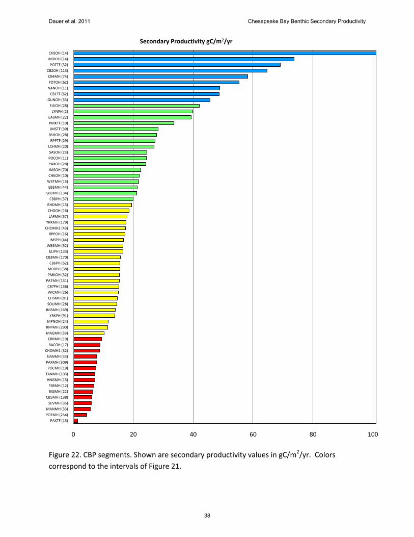
Figure 22. CBP segments. Shown are secondary productivity values in gC/m2/yr. Colors

correspond to the intervals of Figure 21.

0 20 40 60 80 100

PAXTF (13)

POTMH (254)

MANMH (33)

SEVMH (35)

CB5MH (138)

BIGMH (22)

FSBMH (12)

HNGMH (13)

TANMH (103)

POCMH (19)

PAXMH (309)

NANMH (33)

CHOMH1 (32)

BACOH (17)

CRRMH (19)

MAGMH (33)

RPPMH (290)

MPNOH (24)

YRKPH (91)

JMSMH (169)

SOUMH (28)

CHSMH (81)

WICMH (26)

CB7PH (136)

PATMH (131)

PMKOH (32)

MOBPH (38)

CB6PH (62)

CB3MH (170)

ELIPH (133)

WBEMH (52)

JMSPH (44)

RPPOH (16)

CHOMH2 (43)

YRKMH (179)

LAFMH (57)

CHOOH (16)

RHDMH (15)

CB8PH (37)

SBEMH (134)

EBEMH (44)

WSTMH (15)

CHKOH (10)

JMSOH (70)

PAXOH (28)

POCOH (11)

SASOH (23)

LCHMH (20)

RPPTF (29)

BSHOH (28)

JMSTF (39)

PMKTF (10)

EASMH (22)

LYNPH (2)

ELKOH (28)

GUNOH (33)

CB1TF (62)

NANOH (11)

POTOH (62)

CB4MH (74)

CB2OH (113)

POTTF (32)

MIDOH (14)

CHSOH (14)

Secondary Productivity gC/m2/yr


38

Figure 23. Composite Chesapeake Bay summer DO concentration from 1996 to 2004. Large and small circles represent sample sites. Shading and dot color denotes DO concentration as stated in Figure key.

CBP4MH


39

Figure 24. CB4MH secondary productivity values in gC/m2/yr. A. all water depths. B. Depth ≥ 40 m.

0.01

0.10

1.00

10.00

100.00

1000.00

0 5 10 15 20

Bre

y's

Seco

nd

ary

Pro

du

ctio

n (

g C

/m2/y

r)

Sample Depth (m)

0

5

10

15

20

25

30

35

40

0 5 10 15 20

Bre

y's

Seco

nd

ary

Pro

du

ctio

n (

g C

/m2/y

r)

Sample Depth (m)

A.

B.


40

0

2

4

6

8

10

0 5 10 15 20

Bre

y's

Seco

nd

ary

Pro

du

ctio

n (

g C

/m2/y

r)

Sample Depth (m)

Figure 25. CB4MH secondary productivity values in gC/m2/yr. A.. Depth ≥ 20 m. B. Depth ≥ 10 m.

0

5

10

15

20

0 5 10 15 20

Bre

y's

Seco

nd

ary

Pro

du

ctio

n (

g C

/m2/y

r)

Sample Depth (m)

A.

B.


41

1

10

100

1,000

0 5 10 15 20

Bre

y's

Seco

nd

ary

Pro

du

ctio

n (

g C

/m2/y

r)

Sample Depth (m)

Lower Potomac River (POTMH)

Water Depth

(m)

Mean Secondary

Productivity (gC/m2/yr) n

% of samples with no benthos

5.00 243.00 75 8.0

10.00 43.11 103 39.8

15.00 14.94 48 41.7

20.00 4.96 18 72.2

Figure 26. POTMH secondary productivity values in gC/m2/yr. Productivity is show on a log scale due to the wide range of values. Insert shows average secondary productivity by water depth intervals and the percentage of samples with no benthos.


42

0 20 40 60 80 100

PAXTF (13)

POTMH (254)

MANMH (33)

SEVMH (35)

CB5MH (138)

BIGMH (22)

FSBMH (12)

HNGMH (13)

TANMH (103)

POCMH (19)

PAXMH (309)

NANMH (33)

CHOMH1 (32)

BACOH (17)

CRRMH (19)

MAGMH (33)

RPPMH (290)

MPNOH (24)

YRKPH (91)

JMSMH (169)

SOUMH (28)

CHSMH (81)

WICMH (26)

CB7PH (136)

PATMH (131)

PMKOH (32)

MOBPH (38)

CB6PH (62)

CB3MH (170)

ELIPH (133)

WBEMH (52)

JMSPH (44)

RPPOH (16)

CHOMH2 (43)

YRKMH (179)

LAFMH (57)

CHOOH (16)

RHDMH (15)

CB8PH (37)

SBEMH (134)

EBEMH (44)

WSTMH (15)

CHKOH (10)

JMSOH (70)

PAXOH (28)

POCOH (11)

SASOH (23)

LCHMH (20)

RPPTF (29)

BSHOH (28)

JMSTF (39)

PMKTF (10)

EASMH (22)

LYNPH (2)

ELKOH (28)

GUNOH (33)

CB1TF (62)

NANOH (11)

POTOH (62)

CB4MH (74)

CB2OH (113)

POTTF (32)

MIDOH (14)

CHSOH (14)


Figure 27. CBP segments and low dissolved oxygen. Shown are secondary productivity values in

gC/m2/yr. Colors correspond to the intervals of Figure 21. Segments with no color and cross

hatching have mean summer dissolved oxygen levels <5 mg/l.


43

0 20 40 60 80 100

PAXTF (13)

POTMH (254)

MANMH (33)

SEVMH (35)

CB5MH (138)

BIGMH (22)

FSBMH (12)

HNGMH (13)

TANMH (103)

POCMH (19)

PAXMH (309)

NANMH (33)

CHOMH1 (32)

BACOH (17)

CRRMH (19)

MAGMH (33)

RPPMH (290)

MPNOH (24)

YRKPH (91)

JMSMH (169)

SOUMH (28)

CHSMH (81)

WICMH (26)

CB7PH (136)

PATMH (131)

PMKOH (32)

MOBPH (38)

CB6PH (62)

CB3MH (170)

ELIPH (133)

WBEMH (52)

JMSPH (44)

RPPOH (16)

CHOMH2 (43)

YRKMH (179)

LAFMH (57)

CHOOH (16)

RHDMH (15)

CB8PH (37)

SBEMH (134)

EBEMH (44)

WSTMH (15)

CHKOH (10)

JMSOH (70)

PAXOH (28)

POCOH (11)

SASOH (23)

LCHMH (20)

RPPTF (29)

BSHOH (28)

JMSTF (39)

PMKTF (10)

EASMH (22)

LYNPH (2)

ELKOH (28)

GUNOH (33)

CB1TF (62)

NANOH (11)

POTOH (62)

CB4MH (74)

CB2OH (113)

POTTF (32)

MIDOH (14)

CHSOH (14)


Figure 28. CBP segments and high urban land-use. Shown are secondary productivity values in

gC/m2/yr. Colors correspond to the intervals of Figure 21. Segments with no color and cross

hatching are located in either the Maryland Western Tributaries benthic stratum or the

Elizabeth River watershed.


44

4

40

0.75 7.5 75

Be

nth

ic S

eco

nd

ary

Pro

du

ctiv

ity

(gC

/m2

/yr)


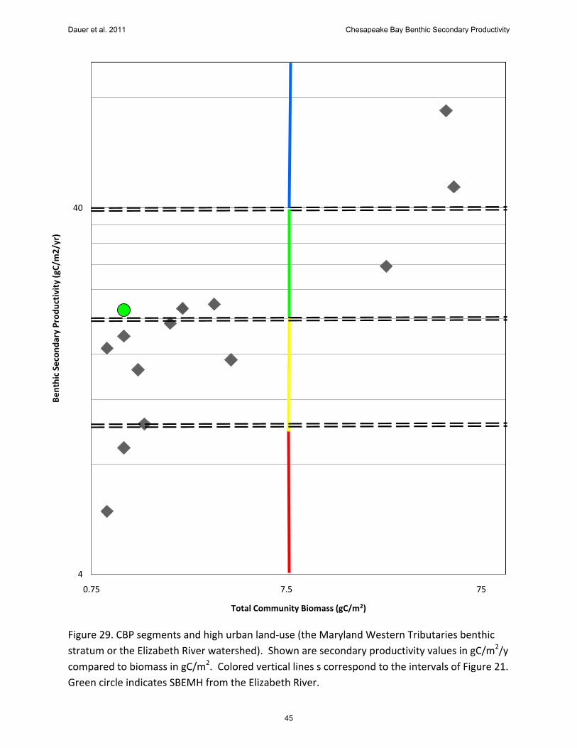
Figure 29. CBP segments and high urban land-use (the Maryland Western Tributaries benthic

stratum or the Elizabeth River watershed). Shown are secondary productivity values in gC/m2/y

compared to biomass in gC/m2. Colored vertical lines s correspond to the intervals of Figure 21.

Green circle indicates SBEMH from the Elizabeth River.


45

0

5

10

15

20

25

JMSMH POTMH PATMH SBEMH

Bre

y's

20

01

Mo

del

Pro

du

ctio

n (

gC/m

2/y

r)

0.00

1.00

2.00

3.00

4.00

5.00


Tota

l co

mm

un

ity

bio

mas

s (g

C/m

2)

Figure 30. Mean secondary production (gC/m2/yr) comparing JMSMH (James River mesohaline), POTMH (lower Potomac River mesohaline), PATMH (Patapsco River) and SMEMH (Southern Branch of the Elizabeth River).

Figure 31. Mean standing stock biomass (gC/m2)) comparing JMSMH (James River mesohaline), POTMH (lower Potomac River mesohaline), PATMH (Patapsco River) and SMEMH (Southern Branch of the Elizabeth River).


Benthic Biomass


46

0

2,000

4,000

6,000

8,000

10,000


Tota

l Co

mm

un

ity

Ab

un

dan

ce (

#/m

2)

1.0

2.0

3.0


Ben

thic

IBI

Figure 32. Mean community abundance comparing JMSMH (James River mesohaline), POTMH (lower Potomac River mesohaline), PATMH (Patapsco River) and SMEMH (Southern Branch of the Elizabeth River). .

Figure 33. Mean B-IBI comparing JMSMH (James River mesohaline), POTMH (lower Potomac River mesohaline), PATMH (Patapsco River) and SMEMH (Southern Branch of the Elizabeth River).

Community Abundance

B-IBI


47

0.00

2.00

4.00

6.00

8.00

10.00

12.00

14.00


Nu

mb

er o

f sp

ecie

s p

er s

amp

le

0.00

0.50

1.00

1.50

2.00

2.50


Shan

no

n-W

ein

er

Ind

ex

Figure 34. Mean species per sample comparing JMSMH (James River mesohaline), POTMH (lower Potomac River mesohaline), PATMH (Patapsco River) and SMEMH (Southern Branch of the Elizabeth River). .

Figure 35. Mean Shannon Index comparing JMSMH (James River mesohaline), POTMH (lower Potomac River mesohaline), PATMH (Patapsco River) and SMEMH (Southern Branch of the Elizabeth River).

Species per sample



48

20

40

60

80

100

120

140

1.5 2.0 2.5 3.0 3.5 4.0

Be

nth

ic S

eco

nd

ary

pro

du

ctiv

ty (

gC/m

2/y

r

B-IBI

Figure 36. CBP segment secondary productivity values in gC/m2/yr and the B-IBI. A. All segments. B. Segments in the two highest productivity categories > 20 and >40 gC/m2/yr

A.

B.

0

20

40

60

80

100

120

140

1.5 2.0 2.5 3.0 3.5 4.0

Be

nth

ic S

eco

nd

ary

pro

du

ctiv

ty (

gC/m

2/y

r

B-IBI


49

Appendix A. Conversion factors used to estimate energetic content of ash free dry weight (AFDW) of individual taxa. An * indicates a higher level taxonomic group conversion factor was used for the group (e.g. Mollusca for Scaphopoda). A ** indicates the general Annelida conversion factor was applied. A H indicates the conversion factor for Crustacea was applied. AI indicates the conversion factor for Ascidacea was applied.

Phylogenetic Group Conversion

Factor (J per mg

AFDW)

Anthozoa 24.46 Annelida 23.33 Mollusca 23.04

Gastropoda 23.63 Polyplacophora 23.27 Bivalvia 22.79 Scaphopoda* 23.04 Cephalopoda 22.03

Arthropoda Crustacea 22.57

Amphipoda 22.74 Cephalocarida* 22.57 Cumacea 22.74 Decapoda 22.26 Isopoda* 22.74 Mysidacea 23.00 Stomatopoda 22.57 Tanaidacea* 22.57

MerostomataH 22.57 Insecta (General) 23.81

Coleoptera 23.81 Collembola 23.81 Chironomidae 23.44 Diptera 23.81 Ephemeroptera 26.07 Megaloptera 23.81 Odonata 23.65 Plecoptera 23.81 Trichoptera 24.12

Echinodermata Asteroidea 20.81 Ophiuroidea 21.75 Echinoidea 20.53 Holothuroidea 22.95

Chordata Ascidiacea 19.01 CephalochordataI 19.01

Miscellaneous groups Nemertina** 23.33 Echiurida** 23.33 Phoronida** 23.33 Sipuncula** 23.33


50

Appendix B. Comparison of benthic secondary productivity BCS of this study to Diaz and Schaffner

(1990) (D & S). For euhaline habitat the D&S value was used for both the Brey and Edgar estimates of

our study.

Habitat Type and Area

Diaz & Schaffner (1990)

Present Study Area weighed BSC

Total Habitat Productivity (metric tons of C/yr)

Major habitat

Area km2

% of Habitat

Mean BSC

Area weighted

BSC

ODU Edgar

ODU Brey

D & S ODU

Brey’s ODU

Edgar’s

Tidal Freshwater Mud 455 0.80 1.8 1.44

Sand 102 0.18 145.5 26.17 Mixed 10 0.02 289.2 5.10 Total area 567

32.72 126.28 32.44 18,552 18,396 71,603

Oligohaline Mud 496 0.79 14.4 11.32


15.62 151.11 36.00 9,854 22,714 95,351

Low

Mesohaline Mud 393 0.75 14.4 10.74

Sand 98 0.19 41.0 7.62 Mixed 36 0.06 10.8 0.74 Total area 527 19.10 81.81 24.55 10,066 12,937 43,113

High

Mesohaline Mud 1525 0.48 8.1 3.88

Sand 1388 0.44 8.8 3.84 Mixed 268 0.08 25.0 2.11 Total area 3181 9.83 16.00 12.00 31,267 38,172 50,896

Polyhaline Mud 509 0.18 9.0 1.64


24.78 22.00 15 69,016 41,775 61,270

Euhaline Mud 148 0.16 17.2 2.69

Sand 768 0.81 5.7 4.63 Mixed 29 0.03 28.6 0.88 Total area 945 8.20 7,753 7,753 7,753

Total for Chesapeake Bay 146,507 141,746 329,986


51

Date post:	01-Sep-2019
Category:	Documents
Upload:	others
View:	1 times
Download:	0 times

Llansó Diaz - Old Dominion...

Documents