26
Superstructure Test, Feb. 2002 Stefan Simrock DESY LLRF for Superstructure Test Stefan Simrock DESY

Superstructure Test, Feb. 2002 Stefan Simrock DESY
LLRF for Superstructure Test
Stefan Simrock
DESY
Superstructure Test, Feb. 2002 Stefan Simrock DESY
LLRF for Superstructure (SS) Test
• RF Control - Separate klystron for SS- and 8 cav. cryomodule- Split 24 cav. LINAC system (24 cav.) in 2 x 8 cav. systems
... 8 probes for 2 x 2x7-cell cavity superstructure - control vector sum of 2 SS cavities - implement bandpass filter at downconverter output - modify LO tables for continuous phase shift - remote controlled waveguide tuners
• RF diagnostic - precise detuning measurements ... for cavity field flatness, microphonics, Lorentz force - high resolution and wide band gradient detection ... measure excitation of passband modes - measurement of IQ or A&P transfer function with lock-in
Superstructure Test, Feb. 2002 Stefan Simrock DESY
LLRF Measurements
• RF Control Performance - gradient and phase stability ... rf and beam energy measurements ... noise sources (beam, microphonics, Lorentz force) ... Adaptive feedforward - Loop stability with/without bandpass filter
• Cavity Tuning - field flatness - resonance frequency
• Other RF measurements - excitation of passband modes by rf and beam - gradient and phase calibration (beam based)
Superstructure Test, Feb. 2002 Stefan Simrock DESY
LLRF Parameters
• Operational - Medium (15 MV/m) and low gradient (2.5 MV/m) ... for ACC1(SS) and ACC2 - Long beam pulses ( up to 8 mA, 800 µs) ... 1 MHz and 54 MHz with current modulation
• Expected field stability with adaptive feedforward - ∆Eacc < 0.02 MV/m - ∆φ < 0.05 deg. (15 MV/m), 0.3 deg. (2.5 MV/m) Note : assumes ∆Ib/Ib< 5% within bunch train at 8 mA
∆Ib/Ib< 0.5% pulse to pulse at 8 mA
Superstructure Test, Feb. 2002 Stefan Simrock DESY
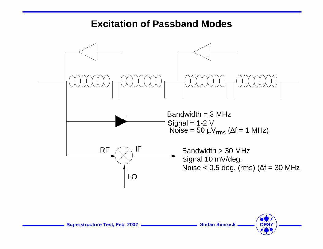
Excitation of Passband Modes
LO
RF
Bandwidth = 3 MHz
Noise = 50 µVrms (∆f = 1 MHz)Signal = 1-2 V
IF Bandwidth > 30 MHzSignal 10 mV/deg.Noise < 0.5 deg. (rms) (∆f = 30 MHz
5.8/ Generator Power 63
1275 1280 1285 1290 1295 1300 1305−80
−60
−40
−20
0
20
40
f [MHz]
ampl
itude
(ce
ll #1
) [d
BA
]ππ8
9π19
π29 π3
9 π49 π7
9π69π5
9
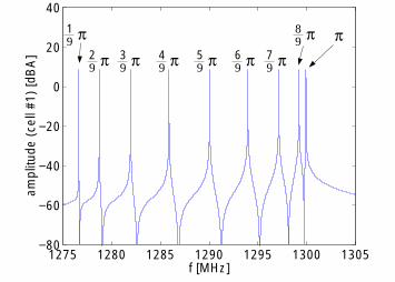
Figure 5.9: Calculated resonance spectrum of the TM010 modes in a TESLA 9-cell cavity.Shown is the steady state amplitude of the eld in cell #1 as a function of the frequency of
the driving RF generator (Kcc = 1:9%, !(1)0 =(2) = 1:276 GHz, Q
(1)0 = 1010, Q
(1;1)e;1 = 105).
5.8 Generator Power
When calculating the generator power by means of the equivalent cavity circuitmodel, we have to take into account, that this model does not include the transmis-sion line, the circulator and the coupler between the generator and the cavity, seegure 5.10. In the simplied cavity model the external load is modelled by the trans-formed waveguide impedance Re = n2Zt for a coupler transformation ratio 1 : n.We have to distinguish carefully between the generator current ~Ig in the model in-cluding the transmission line and the ctitious generator current Ig in the simpliedcavity model. To illustrate the dierence between these currents, we assume thatthe external load is matched to the wall losses according to n2Zt = R0 and thatthe single cell cavity (see gure 5.10) is driven on resonace, i.e !2
g = 1=(LC1). Wewill nd that for these conditions the eld in the cavity is maximized for a givengenerator current. Accordingly, as is well known, all generator power is transferredto the cavity. From gure 5.10 (a) we nd that the cell current I1 is then given by
I1 =1
n~Ig ; (5.108)
since the LC series has zero impedance for !2g = 1=(LC1). Recall that I1 is repre-
senting the eld amplitude in the cell, see (5.84). However, for the simplied modelwe have
I1 =1
2Ig ; (5.109)
6.2/ Amplitude Prole Measurements 85
of the cell. Note that a bead-pull measurement gives absolut values jv(j)b j.It is discussed above that the frequency shift Æf
(j)bead is usually determined by mea-
suring the frequency shift fph for tracking a constant phase. We shall see that
fph and Æf(j)bead are in good agreement for 7-cell and 9-cell cavities, as long as the
two antennas are mounted at opposite end-cells. Accordingly measuring fph is thestandard procedure to determine the amplitude proles of the TM010 eigenmodesin TESLA multicell cavites. The eigenmode prole of the accelerating mode thenneeds to be tuned for homogeneity.It is important to note, that the rst order perturbation approximation (6.11) isused to determine the mode amplitude proles. More accurately we have for theperturbated eigenvalues in a second order perturbation approach
Æ(j)bead = ((j))0 (j) Æbead
v(j)b
2+Xr 6=j
1
(j) (r)
Æbeadv
(j)b v
(r)b
2: (6.12)
As before we consider that the metal bead is in the center of cell b. To ensure thatthe second order term in (6.12) can be neglected, the frequency perturbation dueto the bead has to be suÆcient small. From (6.4) and (6.12) we nd the conditionÆfb fmodes. We will see later in this section, that a perturbation Æfb < 100 kHzshould be used for an accurate bead-pull measurement.The amplitude proles measurement in superstructures needs to be studied morecarefully. The reason for this is, that the spacing of modes is signicantly smallerin a superstructure than in a TESLA 9-cell cavity. Accordingly we have to takeinto account, that the modes overlap at room temperature (see gure 6.4), which isperturbing the bead-pull measurement. Figure 6.5 shows measured on-axis prolesfor selected TM010 resonances of a 27-cell prototype superstructure. The measured
1293 1294 1295 1296 1297 1298 1299 1300−70
−60
−50
−40
−30
−20
−10
0
fg [MHz]
ampl
itude
(ce
ll #1
4)
[dB
A]
π -
π m
ode
6 7π
- π
mod
e
6 7π
- 0
mod
e
5 7π
- π
mod
e
5 7π
- 0
mod
e
π -
0 m
ode
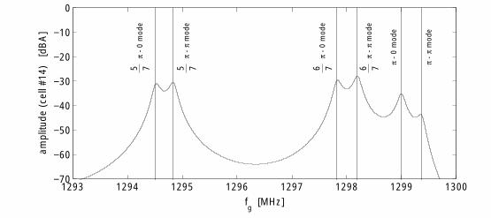
Figure 6.4: Calculated resonance spectrum of the higher frequency TM010 modes in a
TESLA 2 7-cell superstructure at room temperature (Q(1)0 = 104). Shown is the steady
state amplitude of the eld in cell #14 as function of the driving RF generator frequency.The vertical lines mark the eigenfrequencies of the TM010 eigenmodes.
98 Chapter 6/ Amplitude Prole Measurement and Tuning
has been assembled. Figure 6.16 (a) shows the bead-pull amplitude prole of theaccelerating 0 mode, measured after small frequency corrections of the individualcavities (each cavity in a superstructure is equipped with its own frequency tuningsystem). By comparing the measured cell amplitude prole with a simulation for a
0 1000 2000 3000 40000
0.5
1
1.5
2
0 1000 2000 3000 40000
0.5
1
1.5
√| d
f | /
(1kH
z)
√| d
f | /
(1kH
z)
z [mm]
z [mm]
(a)
(b)
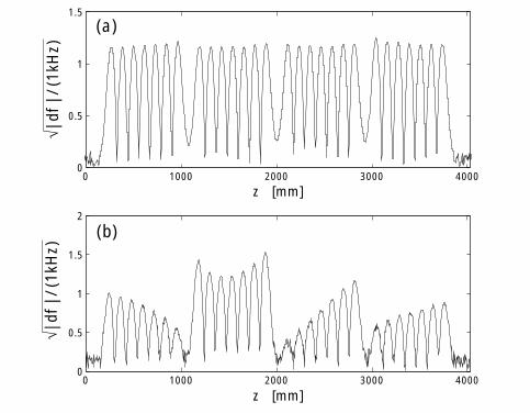
Figure 6.16: Bead-pull resultsqjÆfphj=1kHz on the 47-cell copper model superstructure,
see also gure 9.2. (a) Accelerating 0 mode after small frequency corrections of theindividual cavities. The input antenna is placed at cell #1 and the output antenna at cell#28. Compare to gure 6.12. (b) Same as before, but with cavities detuned to permithigh-power-processing of the second cavity. The rst cavity is detuned by +25 kHz andthe second cavity by -200 kHz.
perfectly tuned superstructure (see gure 6.12) it is found that the achieved ampli-tude homogeneity of the accelerating 0 eigenmode is better than 95 %.High-power-processing is often used to improve the eld performance of supercon-ducting cavities while there are installed in an accelerator [Pad 98]. For the high-power-processing of a superstructure it is desirable to process the cavities of thestructure successively, to reduce the maximum power transferred by the input cou-pler. By proper detuning of the superstructure cavities the dominating part of theinput power can be transferred to one of the cavities. As example, the gure 6.16(b) shows a bead-pull prole on the 4 7-cell copper superstructure with cavitiesdetuned to permit processing of the second cavity.Tuning of the superstructures for the TESLA collider
Based on the promising experience with the 2 7-cell prototypes and the 4 7-cellcopper model, it is proposed to use the pre-tuning procedure also for the TESLA
114 Chapter 7/ Transient Behaviour and Bunch-to-Bunch Energy Variation
1 5 9 1310
−6
10−4
10−2
100
102
R/Q
[Ω
]
TM010 mode #
π-0 modeπ-0 modeπ-0 mode73
75
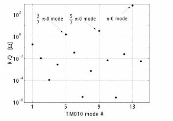
Figure 7.5: (Rsh=Q0)(l) values of the TM010 modes of a 2 7-cell superstructure, as calcu-
lated from equation (7.12). It is considered that (Rsh=Q0)n values of the four end-cells are2=3 of the value for a center cell [Sek 00]. The 0 mode is the accelerating eigenmode.
2 7-cell structure, as calculated from equation (7.12). The accelerating ( 0)mode (l = 13) has the largest (Rsh=Q0)
(13) = 729 . The (37 0) mode and the
(57 0) mode will also interact with the beam, but their (Rsh=Q0)
(l) is a few 103
of the fundamental mode (Rsh=Q0)(13).
The resulting energy variation of the bunches has been calculated by computer sim-ulations. For this purpose a TESLA-type bunch train of 2820 bunches is considered.The rst bunch of the train is injected at tf = 2Q(13;13)
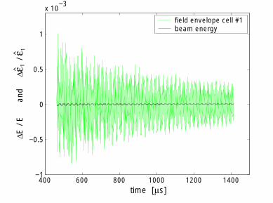
e =!(13)ln(2) = 462 s. Thebunches are 337 ns spaced [TDR 01]. Each bunch is composed of 2 1010 relativisticelectrons. Figure 7.6 shows the computed bunch-to-bunch energy variation as wellas the uctuation of the eld envelope in cell #1. The eld is sampled immediatelybefore a bunch is injected into the superstructure, thus showing the modulation ofthe accelerating voltage in this cell as "seen" by the beam. It is found, that thebunch-to-bunch energy gain variation is more than one order of magnitude smallerthan the uctuation of the individual elds in the cells. The modulation of the eldamplitude in the cell is caused by the non-fundamental modes, which are excited bythe generator and the beam. The amplitude of excitation depends on the frequencyof the modes, their time constant and the generator and beam coupling to themodes, see (5.143) and (7.13). Figure 7.7 shows the eld energy U (l) = 1
2"0a
(l)(a(l))
of selected modes as a function of time. With increasing frequency separation to thegenerator frequency fg = 1:3 GHz, the mode excitation by the generator current is
getting smaller. For a single bunch the amplitude coeÆcient a(l)b induced by the
bunch is proportional to the square root of the (Rsh=Q0)(l) of mode l, see equation
(7.12) and (7.13). The excitation by a bunch train depends also on the distance be-tween the eigenfrequencies and the Fourier components of the bunched beam, sincethis determines how the bunch-induced transients add up. For the parameters of thecomputation discussed here it is found, that beside the fundamental mode mainlythe (3
7 0) mode of the 2 7-cell superstructure is excited by the beam. This is
7.2/ Bunch-to-Bunch Energy Variation 115
400 600 800 1000 1200 1400−1
−0.5
0
0.5
1
x 10−3
time [µs]
field envelope cell #1beam energy
∆E /
E
an
d
∆ε
/ ε
11
^^
Figure 7.6: Computed energy gain variation and modulation of the eld envelope in the
rst cell for a 27-cell superstructure (Kcc = 0:01934, Krr = 3:6104, Q(13;13)e = 2:733106,
f (13) = 1:3 GHz). The nominal energy gain is 37.9 MeV. The envelope eld is sampledimmediately before the injection of the bunches. The used (Rsh=Q0)
(l) values of the TM010
modes are shown in gure 7.5.
due to the small, but non-vanishing (Rsh=Q0)(5) value of the (3
7 0) mode and its
spacing of only 46 kHz to the nearest beam harmonics.Figure 7.6 shows that the bunch-to-bunch energy gain variation is more than anorder of magnitude smaller than the uctuation of the accelerating elds of the in-dividual cells. The reason for this is that the bunches are accelerated by the sumof the accelerating elds of all cells. This sum nearly vanishes for all eigenmodesexcept for the fundamental ( 0) mode. This cancellation is the physical originof the small (Rsh=Q0)
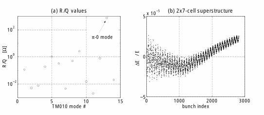
(l) values of the non-fundamental modes shown in gure 7.5.Figure 7.8 compares the individual cell eld uctuation with the uctuation of thetotal accelerating voltage in the 2 7-cell superstructure. The total acceleratingvoltage is mainly modulated by the bunch-induced transients of the acceleratingmode and the relling between the bunches. The computed energy gain variationfor the 2 7-cell superstructure is shown in gure 7.9. The nominal energy gainis 37.9 MeV. It is found, that the bunch-to-bunch energy variation for the wholeTESLA bunch-train in this structure is predicted to be smaller than 5 105, thuswell below the intra-bunch energy spread. This demonstrates, that the energy owfrom the input coupler through the whole 2 7-cell superstructure is suÆcient toreplenish the stored energy in all cells without causing unacceptable energy spread.The variation in energy becomes smaller at the end of the bunch-train due to thedecay of the interfering modes. As discussed above, the uctuation is dominated bythe (3
7 0) mode for the parameters used in this simulation; see also gure 7.7.
Accordingly by shifting the eigenfrequency of this mode such, that the distance to
118 Chapter 7/ Transient Behaviour and Bunch-to-Bunch Energy Variation
1411 1412 1413 1414−1
−0.5
0
0.5
1x 10
−3
time [µs]
cell #1 cell #13
0 1000 2000 3000−5
0
5x 10
−5
bunch index
∆ E
/ E
2kc=0.01934
2kc=0.019
bunch injectionbunch ...
∆ε
/ εn
n^
^
(a) field amplitude in a cell (b) energy gain variation
Figure 7.10: Computed modulation of the eld amplitude and the energy gain in a 2 7-
cell superstructure (Krr = 3:6 104, Q(13;13)e = 2:733 106, f (13) = 1:3 GHz). The nominal
energy gain is 37.9 MeV. The cell-to-cell coupling factor is shifted from Kcc = 0:019 toKcc = 0:019 to shift the 3
7 0 mode eigenfrequency by 258 kHz. (a) Fluctuation of theabsolute value of the eld envelope coeÆcient of cell #1 and #13. Shown are the last 3 sof the bunch train. (b) Bunch-to-bunch energy gain variation for a TESLA bunch-trainof 2820 bunches (cell-to-cell coupling factor Kcc = 0:01934 and Kcc = 0:019).
0 1000 2000 3000−5
0
5x 10
−5
∆E /
E
0 5 10 15
10−2
100
102
TM010 mode #
R/Q
[Ω
]
bunch index
π-0 mode
(a) R/Q values (b) 2x7-cell superstructure
Figure 7.11: Interaction between the beam and the TM010 modes in a 27-cell superstruc-ture. (a) (Rsh=Q0)
(l) values of the eigenmodes calculated by a numerical code [Sek 94].Computation done by J. Sekutowicz, DESY [Sek 00]. (b) Computed bunch-to-bunch en-ergy gain variation for a train of 2820 bunches (TESLA parameters). Nominal energy gain35.6 MeV. Computation done by M. Ferrario, INFN, with HOMDYN [Fer 96].
8CHAPTER
8 RF Field Control for Superstructures
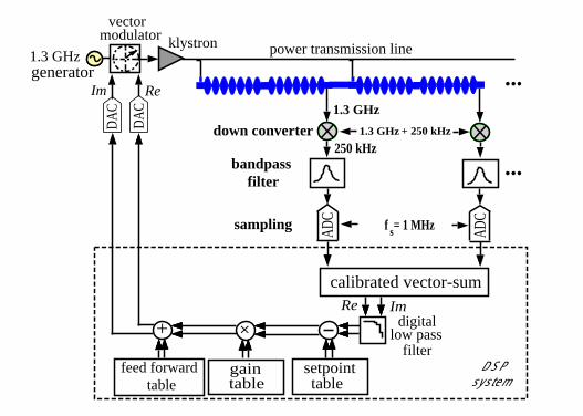
In the previous chapters it has been discussed how the relatively small TM010 eigen-frequency spacing in a superstructure aects the amplitude homogeneity tuning andthe bunch-to-bunch energy spread. In this chapter we study the consequences of thesmall eigenfrequency spacing for the RF control system. For the 9-cell cavites atthe TESLA-Test-Faciliy a digital RF control system has been developed [Schi 98],as brie y described in section 2.2. We will nd that an additional analog bandpasslter in the eld detection (see gure 8.1) is suÆcient to adapt the TTF controlsystem for superstructures and to guarantee stability of the control loop.
ReIm
klystron
vectormodulator
1.3 GHz
1.3 GHz + 250 kHz
power transmission line
DA
C
DA
C
...
ADC
f = 1 MHzs
calibrated vector-sum
DSPsystem
++ digitallow pass
filter
ImRe
250 kHz
ADC
setpointtable
gaintable
feed forward table
...bandpass filter
down converter1.3 GHz
generator
sampling
Figure 8.1: Schematic view of the TTF RF control system [Schi 98], as adapted for eldstabilization in superstructures. The down-converted pick-up antenna signal is lteredby a bandpass lter before it is sampled with an ADC (Analog-Digital-Converter). Thecontrol system is stabilizing the vector-sum of the elds of several superstructures.
8.1/ Accelerating Field Detection 121
8.1 Accelerating Field Detection
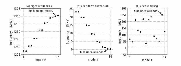
In the TTF control system [Schi 98] the real and imaginary components of the cavityeld are stabilized. The fundamental mode 1.3 GHz signal of a pick-up antennaclose to one end-cell of each cavity is down-converted to an intermediate frequency(IF) of 250 kHz, which contains the amplitude and phase information of the RFsignal. Accordingly the eigenfrequencies f (l) of the non-fundamental TM010 modesare converted to
f(l)if = flo f (l) = 1:3 GHz + 250 kHz f (l) : (8.1)
Here flo is the frequency of a local oscillator, which serves as the frequency osetin the down-conversion, see [Schi 98] for details. Figure 8.2 (a) shows the TM010
eigenfrequencies of a 2 7-cell superstructure. The down-converted frequencies ofthe modes are shown in gure 8.2 (b). According to the 1 MHz electron-bunch
1 14−50
0
50
100
150
200
250
300
mode #
freq
uenc
y
[kH
z]
1 14
0
5
10
15
20
25
mode #
freq
uenc
y
[MH
z]
1 141275
1280
1285
1290
1295
1300
1305
mode #
freq
uenc
y
[MH
z]fundamental mode fundamental mode
fundamental mode
(a) eigenfrequencies (b) after down conversion (c) after sampling
Figure 8.2: Frequencies in the eld detection signal of a 2 7-cell superstructure. (a)
TM010 eigenfrequencies. (b) Frequencies f(l)if after down-conversion. (c) Frequencies after
down-conversion and sampling with 500 kHz.
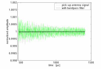
repetition rate at the TTF linac, the down-converted signal is sampled with a rateof 1MHz. This yields four samples per period of the 250 kHz IF signal. Sincethe samples are 90Æ apart, two subsequent voltages can be taken as the real andthe imaginary parts of a complex eld vector, which is representing the accleratingeld of the fundamental mode. Accordingly the real and the imaginary parts areupdated every 2 s, corresponding to an eective sampling rate of 500 kHz. Alsothe eld of non-fundamental modes is measured, down-converted and sampled with500 kHz rate. Due to aliasing, all IF frequencies above 250 kHz are mapped ontofrequencies between 0 to 250 kHz, see gure 8.2 (c). The sampled eld probe signalis uctuating on account of the non-fundamental modes, see gure 8.3. However,the accelerating voltage experienced by a beam is totally dominated by the funda-mental mode, since the non-fundamental TM010 modes have only small (Rsh=Q0)values, see chapter 7. Thus it is desirable to suppress the pick-up antenna signalof the non-fundamental eigenmodes. To achieve this, analog bandpass lters with
122 Chapter 8/ RF Field Control for Superstructures
a center frequency of 250 kHz and a bandwidth of about 100 kHz to 200 kHz willbe placed after the down-converters, see gure 8.1. These lters do not attenuatethe fundamental mode signal, since its down-converted frequency is 250 kHz, butsuppress the non-fundamental mode signals, see gure 8.3. Note that this suppres-
500 1000 15000.998
0.9985
0.999
0.9995
1
1.0005
1.001
1.0015
1.002
time [µs]
norm
aliz
ed a
mpl
itude
pick−up antenna signalwith bandpass filter
Figure 8.3: Computed amplitude signal of a pick-up antenna close to cell #14 of a 2 7-cell superstructure, which is sampled with to the bunch repetition rate. Shown is theamplitude of the unltered signal, which is uctuating on account of the pick-up signalof the non-fundamental modes. The corresponding bunch-to-bunch energy variation isshown in gure 7.6 (see also gure 7.7). Also shown is the ltered signal (Butterworth 8th
order analog lter with 100 kHz bandwidth).
sion is more important for superstructures than for 9-cell cavites, since the excita-tion of non-fundamental modes by the driving generator is stronger on account ofthe smaller frequency spacing between the fundamental mode and the neighboringTM010 modes. Accordingly in the present control system for the 9-cell cavities atthe TTF linac no analog bandpass lter is needed.
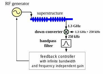
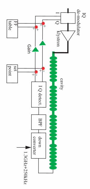
8.2 Stability Analysis
By ltering the measured signal, which is used for controlling of the acceleratingvoltage, robustness and stability of the control loop can be guaranteed. This willbe illustrated in the following for the 2 7-cell prototype superstructure. In or-der to cover the most critical case with respect to stability, an ctive controller isconsidered (see gure 8.4), which provides frequency independent feedback gain.Moreover it is assumed that the generator, which is driving the superstructure, hasalso innite bandwidth. Therefore stability has to be guaranteed by the bandpasslter, since this lter is the only bandwidth limiting element in the control loopbeside the superstructure itself, see gure 8.4. Accordingly if the ctive control loopshown in gure 8.4 is stable, stablility is also guaranteed for the controller, which is
8.2/ Stability Analysis 123
1.3 GHz + 250 kHz
250 kHzbandpass
filter
down-converter1.3 GHz
RF generator
feedback controllerwith infinite bandwidth
and frequency independent gain
superstructure
Figure 8.4: Schematic view of the ctive control loop, which is considered in the stabilityanalysis of the feedback system for superstructures (total delay in the feedback loop: 5 s).
proposed for the superstructures, see gure 8.1. The total delay in the control loopis assumed to be 5 s as it is in the present TTF RF eld control system. A controlloop is stable at a given frequency, if the total phase advance along the loop is amultiple of 2. For this phase advance an oscillation with the considered frequencyis supressed by the negative feedback of the control loop. In the control loop forthe cavity RF eld (see gure 8.1 and 8.4), the phase advance along the loop isadjusted for negative feedback at the frequency of the fundamental mode, since theaccelerating eld needs to be stabilized. However, the phase advance along the loopdepends on the frequency. If the phase advance reaches 180Æ, the negative controlloop feedback is turned into positive feedback. Accordingly the loop is unstable ifits gain at this frequency is larger than one (unity gain, 0 dB).Figure 8.5 (a) shows the computed amplitude of the eld probe signal for the2 7-cell superstructure as function of the generator frequency. Hereby it is con-sidered that the pick-up antenna is close to cell #14 and that the generator currentamplitude is independent of the frequency. After after mixing with flo = 1300:25MHz the fundamental mode frequency 1.3 GHz is mapped to 250 kHz. The com-puted frequency spectrum of the pick-up signal after down-conversion is shown ingure 8.5 (b). Subsequently the down-converted signal is ltered by the bandpasslters (Butterworth 8th order analog bandpass lter with 100 kHz bandwidth), asshown by the lower curve in gure 8.5 (b). The center frequency of the bandpasslter is adjusted to 250 kHz, thus the signal of the fundamental 0 mode is notattenuated, whereas the signal of the non-fundamental TM010 modes is supressed.The lter characteristics of the bandpass lter is shown in gure 8.6 for selectedbandwidths.

124 Chapter 8/ RF Field Control for Superstructures
1.275 1.28 1.285 1.29 1.295 1.3 1.305
−150
−100
−50
0
50
frequency [GHz]
ampl
itude
[dB
A]
104
105
106
107
108
−300
−250
−200
−150
−100
−50
0
50
frequency [Hz]
ampl
itude
[dB
A]
without filterwith filter
(a) pick-up antenna signal before down-conversion
(b) pick-up antenna signal after down-conversion
π-0 modeπ-π mode
π-0 modeπ-π mode π-π mode67
Figure 8.5: Computed TM010 resonance spectrum of a superconducting 2 7-cell su-perstructure for a driving RF generator with constant amplitude (Kcc = 0:019, Krr =
3:6 104, Q(1)0 = 1010, Q
(13;13)e = 2:733 106). (a) Amplitude of the eld probe signal
measured via a pick-up antenna close to cell #14. (b) Field probe signal after mixingwith flo = 1300:25 MHz and ltering (Butterworth 8th order analog bandpass lter with100 kHz bandwidth).

8.2/ Stability Analysis 125
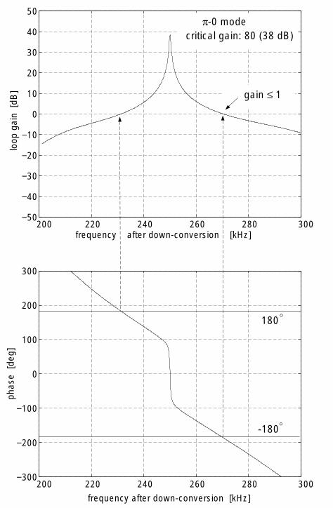
For the control loop shown in gure 8.4 the amplitude of the ltered pick-upantenna signal gives the frequency dependence of the loop gain, since the controllerand the generator are considered to have frequency independent gain. Stability of thecontrol loop requires, that the gain at all frequencies with positive feedback is belowone. Figure 8.7 shows the loop gain and the loop phase advance (minus multiples of2) at frequencies near to the fundamental-mode frequency. It is found that the gain-margin between the gain at the fundamental mode frequency and the frequencieswith positive feedback (180Æ phase advance) is 80 (38 dB) for the parameters ofthe example dicussed here. This gain-margin gives the critical loop gain for the
103
105
107
−250
−200
−150
−100
−50
0
50
frequency [Hz]
ampl
itude
[dB
A]
500 kHz bandwidth200 kHz bandwidth50 kHz bandwidth
103
105
107
−800
−700
−600
−500
−400
−300
−200
−100
0
frequency [Hz]
phas
e [d
eg]
500 kHz bandwidth200 kHz bandwidth50 kHz bandwidth
(a) (b)
Figure 8.6: Computed lter characteristics of Butterworth 8th order analog bandpass lterswith selected bandwidths. The center frequency is 250 kHz. (a) Amplitude response asfunction of frequency. (b) Phase advance as function of frequency.
negative feedback on the fundamental eigenmode eld. However, a loop gain belowbut close to this critical gain results in overshooting and oscillation around a givensetpoint for the accelerating eld [Schi 98]. According to the methode of Ziegler andNichols [Lun 97] the optimal gain Kopt for a proportional gain controller is half ofthe critical gain Kcrit
Kopt = 0:5 Kcrit : (8.2)
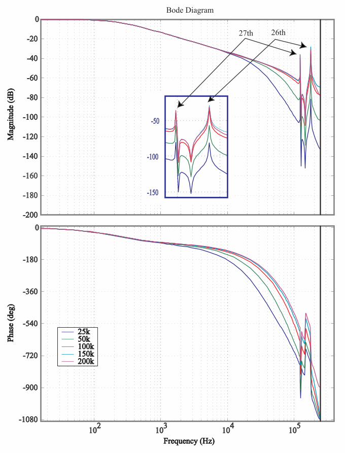
Accordingly for the example shown in gure 8.7 the optimal feedback gain at thefundamental mode frequency is 40.Up to now only frequencies near to the fundamental mode frequencies have beenconsidered in the stability analysis. Figure 8.8 shows the frequency dependence ofthe loop gain for the full frequency range of the TM010 modes for the ctive con-trol loop. It is found that the gain has local maxima at the mode eigenfrequenciesafter down-conversion. The phase advance of the control loop at these frequenciesstrongly depends on the eigenfrequencies and the time delay in the loop. To guaran-tee robustness against parameter uctuations the worst case needs to be considered,i.e. positive feedback at the eigenfrequencies of the non-fundamental modes. Ac-cordingly stability of the control loop requires, that the gain at these frequenciesis below one, as is discussed above. The gain at the eigenfrequencies of the non-
126 Chapter 8/ RF Field Control for Superstructures
200 220 240 260 280 300−300
−200
−100
0
100
200
300
frequency after down-conversion [kHz]
phas
e [d
eg]
200 220 240 260 280 300−50
−40
−30
−20
−10
0
10
20
30
40
50lo
op g
ain
[dB
]
-180°
180°
π-0 modecritical gain: 80 (38 dB)
gain ≤ 1
frequency after down-conversion [kHz]
Figure 8.7: Computed loop gain and phase advance near to fundamental-mode frequencyafter down-conversion for the control loop, which is shown in gure 8.4 (2 7-cell super-
structure, Q(13;13)e = 2:733 106, 5 s loop delay, Butterworth 8th order analog bandpass
lter with 100 kHz bandwidth).

128 Chapter 8/ RF Field Control for Superstructures
104
105
106
107
108
−300
−250
−200
−150
−100
−50
0
50
frequency after down-conversion [Hz]
loop
gai
n [d
B]
π-0 modemax. gain: 210 (46.5 dB)
π-π modemax. gain: ≤1 (0 dB)
incre
ased
feed
back
-gain
Figure 8.8: Computed loop gain of the control loop, which is shown in gure 8.4 as function
of frequency after down-conversion (2 7-cell superstructure, Q(13;13)e = 2:733 106, 5 s
loop delay, Butterworth 8th order analog bandpass lter with 100 kHz bandwidth). Shownis the loop gain for two dierent feedback gains of the controller.
8.3/ Conclusion 129
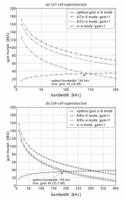
0 50 100 150 200 250 300 350 4000
20
40
60
80
100
120
140
160
180
200
gain
mar
gin
[dB
A]
optimal gain π−0 mode8/9π−0 mode: gain=1 8/9π−π mode: gain=1π−π mode: gain=1
0 50 100 150 2000
20
40
60
80
100
120
140
160
180
200ga
in m
argi
n [d
BA
]
optimal gain π−0 mode6/7π−0 mode: gain=1 6/7π−π mode: gain=1π−π mode: gain=1
optimal bandwidth: 140 kHzmax. gain: 50 (34 dB)
bandwidth [kHz]
bandwidth [kHz]
optimal bandwidth: 190 kHzmax. gain: 60 (35.5 dB)
(a) 2x7-cell superstructure
(b) 2x9-cell superstructure
Figure 8.9: Maximum feedback gain Kfb for the control loop shown in gure 8.4 at thefundamental mode frequency (5 s loop delay) as function of the full bandwidth of theButterworth 8th order analog bandpass lter. The curves show the optimal gain if only thefundamental 0 mode is considered as well as the maximum gain for the stability con-dition Kfb 1 at the frequencies of the neighboring modes. (a) 2 7-cell superstructure.(b) 2 9-cell superstructure.
down
converterB
PFI Q
detect.
IQde-m
odulatorklystroncavity
+ -+ -
set point
+ ++ +
FF table
I Q
1.3GH
z+250kHz
+
Gain
Bode Diagram
Frequency (Hz)
Phas
e (d
eg)
Mag
nitu
de (d
B)
-200
-180
-160
-140
-120
-100
-80
-60
-40
-20
0
102 103 104 105-1080
-900
-720
-540
-360
-180
0
25k50k100k150k200k
26th27th
-150
-100
-50
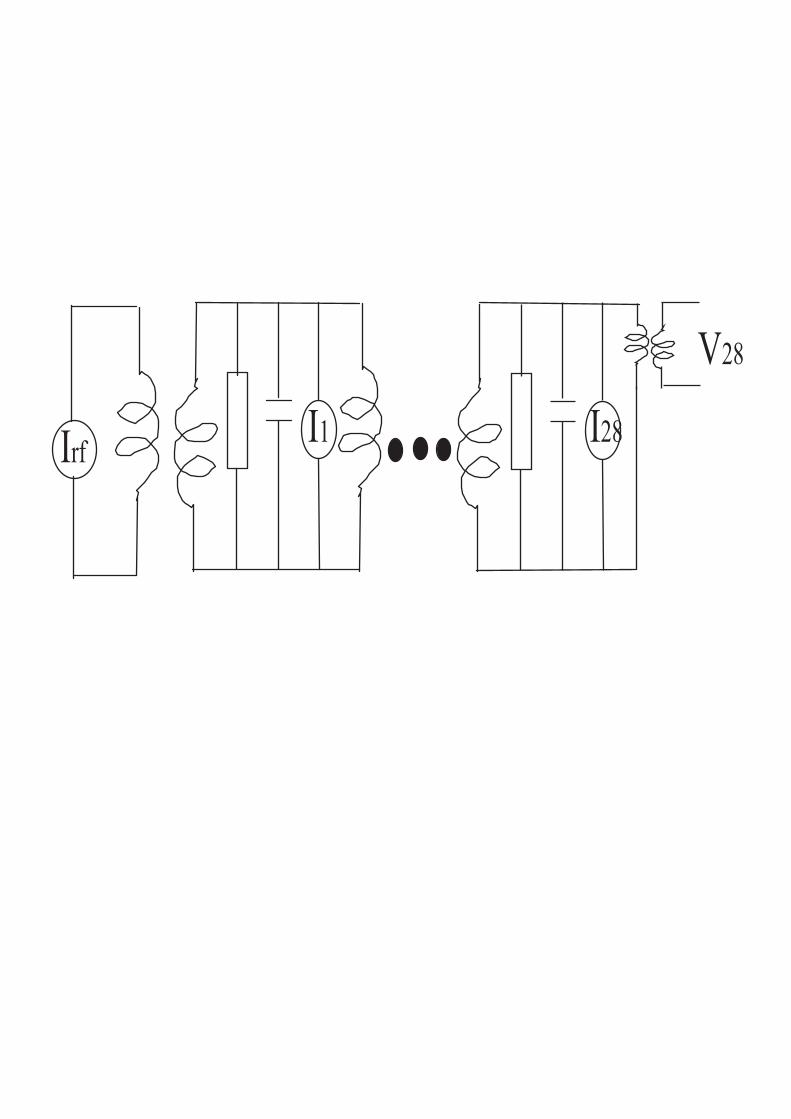
Irf I1 I28
V28

25th24th
26th27th
28th250kHz 250kHz
fLO(1.3GHz+250kHz)
BPFBPF
1.3GHzfrequency
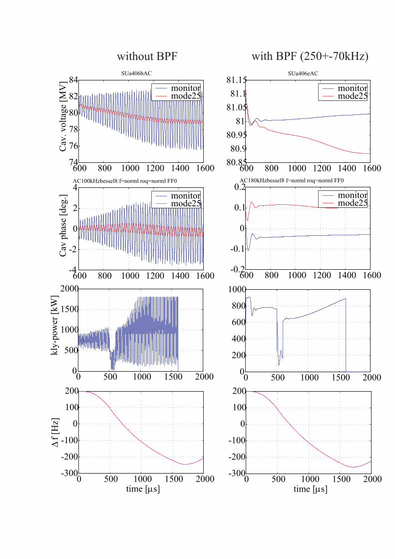
600 800 1000 1200 1400 160074
76
78
80
82
84SUa406bAC
Cav
. vol
tage
[MV
]
monitormode25
600 800 1000 1200 1400 1600-4
-2
0
2
4
Cav
pha
se [d
eg.]
AC100kHzbessel8 f=norml roq=norml FF0
monitormode25
0 500 1000 1500 20000
500
1000
1500
2000
kly-
pow
er [k
W]
0 500 1000 1500 2000-300
-200
-100
0
100
200
time [µs]
∆f [
Hz]
600 800 1000 1200 1400 160080.8580.9
80.9581
81.0581.1
81.15SUa406eAC
monitormode25
600 800 1000 1200 1400 1600-0.2
-0.1
0
0.1
0.2AC180kHzbessel8 f=norml roq=norml FF0
monitormode25
0 500 1000 1500 20000
200
400
600
800
1000
0 500 1000 1500 2000-300
-200
-100
0
100
200
time [µs]
without BPF with BPF (250+-70kHz)
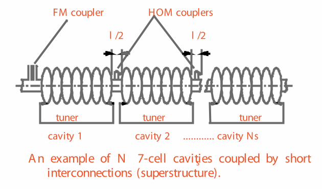
FM coupler HOM couplers
tuner tuner tuner
cavity 1 cavity 2 ............ cavity Ns
l /2 l /2
A n example of N s7-cell cavities coupled by shortinterconnections (superstructure).


