LMI Methods in Optimal and Robust Control

Matthew M. PeetArizona State University

Lecture 1: Introductions

Who Am I?

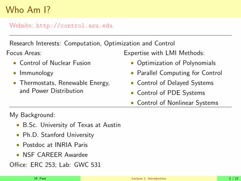
Website: http://control.asu.edu

Research Interests: Computation, Optimization and Control

Focus Areas:

• Control of Nuclear Fusion

• Immunology

• Thermostats, Renewable Energy,and Power Distribution

Expertise with LMI Methods:

• Optimization of Polynomials

• Parallel Computing for Control

• Control of Delayed Systems

• Control of PDE Systems

• Control of Nonlinear Systems

My Background:

• B.Sc. University of Texas at Austin

• Ph.D. Stanford University

• Postdoc at INRIA Paris

• NSF CAREER Awardee

Office: ERC 253; Lab: GWC 531

M. Peet Lecture 1: Introduction 2 / 22

MAE 598: LMI Methods in Optimal and Robust ControlReferences

Required: LMIs in Control Systemsby Duan and Yu

LMIs in Systems and Control Theoryby S. BoydLink: Available Online Here

Linear State-Space Control Systemsby Williams and Lawrence

Convex Optimizationby S. BoydLink: Available Online Here

Link: Entire Course Online Here

M. Peet Lecture 1: Introduction 3 / 22

MAE 598: LMI Methods in Optimal and Robust Control

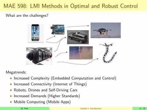
What are the challenges?

Megatrends:

• Increased Complexity (Embedded Computation and Control)

• Increased Connectivity (Internet of Things)

• Robots, Drones and Self-Driving Cars

• Increased Demands (Higher Standards)

• Mobile Computing (Mobile Apps)

M. Peet Lecture 1: Introduction 4 / 22

MAE 598: LMI Methods in Optimal and Robust Control

What are the challenges?

Megatrends:

• Increased Complexity (Embedded Computation and Control)

• Increased Connectivity (Internet of Things)

• Robots, Drones and Self-Driving Cars

• Increased Demands (Higher Standards)

• Mobile Computing (Mobile Apps)

2019-08-27

Lecture 1Introduction

MAE 598: LMI Methods in Optimal and RobustControl

• Sources of Complexity: Smarter devices have more complicated action spaces;Ubiquitous computation; Cheap sensors and actuators;

• Sources of Connectivity: RFID, bluetooth, low-energy bluetooth, LAN, WiFi,WAN, 5G LTE, GPS, satellite broadband, TDRS, integrated circuits

– Problems: delay, lost packets, noise, loss of signal

• Sources of Demands: Improved Efficiency; Expanded Functionality; UserFriendliness; Reduced Tolerance for Failure.

Challenges for Control in the 21st centuryPrivatization of Space Travel

Challenges

• Safety

• Complexity

• Uncertainty

Links:Blue Origin Successful LandingBlue Origin Successful Landing: Flight 3SpaceX Landing, Second AttemptProton M launch Failure (FCS was for wrong rocket)Kepler Space Telescope

M. Peet Lecture 1: Introduction 5 / 22

Challenges for Control in the 21st centuryUAVs and Drones (Delay, Sampled-Data)

Safe Interaction with

• Crowded Airspace

• Real-Time ObstacleAvoidance

Precision Control with

• Delayed Feedback

x(t) = Ax(t) +Bu(t− τ)

• Lossy Connections

x(t) = Ax(t) +Bu(tk)

Links:X47 Drone Carrier LandingRaff’s TED talk

M. Peet Lecture 1: Introduction 6 / 22

Challenges for Control in the 21st centurySelf-Driving Vehicles

Challenges:

• Safety (Provable)

• Uncertainty (in model,environment)

• Other Drivers (Multi-Agent)

• Obstacles

Self-Driving Vehicles

• Google (Waymo)

• Uber

• Tesla, Mobileye

• Toyota, Nutonomy

Links:Toyota’s Research Expansion in AutomationUber’s self-driving Taxis are in PittsburgSelf-Driving Cars Flood into Arizona

M. Peet Lecture 1: Introduction 7 / 22

Challenges for Control in the 21st centuryInterconnectivity (Decentralized Control)

Surface Coal MineUnderground Coal MineBiomass Power PlantCoal Power PlantGeothermal Power PlantHydroelectric Power Plant

Natural Gas Power PlantNuclear Power PlantOther Power PlantPetroleum Power PlantPumped Storage Power PlantSolar Power Plant

Wind Power PlantPetroleum RefineryBiodiesel PlantEthanol PlantNatural Gas Processing Plant (z)Ethylene Cracker

HGL Market Hub (z)Natural Gas Market Hub (z)Electricity Border CrossingNatural Gas Pipeline Border Crossing

0 30 6015 MilesmNCredits : layer1 : Esri, HERE, DeLorme, MapmyIndia, © OpenStreetMap contributors, and the GIS user community; State Layers : ; layer0 : Esri, HERE,DeLorme, MapmyIndia, © OpenStreetMap contributors, and the GIS user community

Figure: Power Generation and Distribution Map of AZ and Southern CA

M. Peet Lecture 1: Introduction 8 / 22

Challenges for Control in the 21st centuryRobotics (Hybrid and Nonlinear Dynamics, PDE systems)

HARD Robots

• Uncertain Terrain

• Interactions with the environment

If x(t)>0:

x(t) = Ax(t)

If x1(t)=0 AND x2(t)<0: Set

x2(t) = −x2(t)Link:Boston Dynamics, Atlas Mark 3

SOFT Robots

• Infinite Degrees of Freedom

• Material Dynamics

Link:Robotic Worm

M. Peet Lecture 1: Introduction 9 / 22

Challenges for Control in the 21st centuryArduino and Raspberry Pi

Trends:

• Rapid prototyping

• Internet of Things

• Control is Everywhere

Challenges

• Noisy Sensors

• Data-Driven Modeling

• Dynamics with logical switching

x = Ax+Bu(t)

If Occupied=True :

u(t) = K1x(t)

Else : u(t) = K2x(t)

M. Peet Lecture 1: Introduction 10 / 22

MAE 598: LMI Methods in Optimal and Robust Control

This course is on RECENT Developments in Control

• Techniques Developed in the Last 20 years

• Computational MethodsI No Root LocusI No Bode PlotsI No PID (Proportion-Integral-Differential)

We focus on State-Space Methods

• In the time-domain

• We use large state-space matrices

d

dt

x1(t)x2(t)x3(t)x4(t)

=

−1 1.2 −1 .81 0 0 00 1 0 00 0 1 0

x1(t)x2(t)x3(t)x4(t)

+

1 00 10 00 0

[u1(t)u2(t)

]

• We require MatlabI Need robust control toolbox.I Recommend using YALMIP.

Link: Installs YALMIP and some other toolboxes

M. Peet Lecture 1: Introduction 11 / 22

So What is an Automatic Control System???

Well... What is a System?

Definition 1.

A System is anything with Inputs and Outputs

There should ALWAYS be Inputs and Outputs!

• If No Inputs: You can’t change anything.

• IF No Outputs: Then it doesn’t matter anyway.

M. Peet Lecture 1: Introduction 12 / 22

So What is an Automatic Control System???12 - 2 LFTs and stability 2001.11.07.04

2-input 2-output framework

exogenous inputs wz regulated outputs

y sensed outputs actuator inputs uPlant

Inputs

• Actuator inputs u are those inputs to the system that can be manipulated by thecontroller.

• Exogenous inputs w are all other inputs.

Outputs

• Regulated outputs z are every output signal from the model.

• Sensed outputs are those outputs which are accessible to the controller.

Notes

• Objective is to write all specifications in terms of z and w.

In Controls, we separate internal signals from external signals.Output Signals:

• z: Output to be controlled/minimized

• y: Output used by the controller

Input Signals:

• w: Disturbance, Tracking Signal, etc.

• u: Output from controllerI Input to actuator

M. Peet Lecture 1: Introduction 13 / 22

So What is an Automatic Control System???State-Space System

12 - 2 LFTs and stability 2001.11.07.04

2-input 2-output framework

exogenous inputs wz regulated outputs

y sensed outputs actuator inputs uPlant

Inputs

• Actuator inputs u are those inputs to the system that can be manipulated by thecontroller.

• Exogenous inputs w are all other inputs.

Outputs

• Regulated outputs z are every output signal from the model.

• Sensed outputs are those outputs which are accessible to the controller.

Notes

• Objective is to write all specifications in terms of z and w.

A state-space system has the form

x(t) = Ax(t) +B1w(t) +B2u(t)

z(t) = C1x(t) +D11w(t) +D12u(t)

y(t) = C2x(t) +D21w(t) +D22u(t)

x(t) ∈ Rn is the internal state.x ∈ Ln

2 is the internal signal.

M. Peet Lecture 1: Introduction 14 / 22

So What is an Automatic Control System???State-Space System

12 - 2 LFTs and stability 2001.11.07.04

2-input 2-output framework

exogenous inputs wz regulated outputs

y sensed outputs actuator inputs uPlant

Inputs

• Actuator inputs u are those inputs to the system that can be manipulated by thecontroller.

• Exogenous inputs w are all other inputs.

Outputs

• Regulated outputs z are every output signal from the model.

• Sensed outputs are those outputs which are accessible to the controller.

Notes

• Objective is to write all specifications in terms of z and w.

A state-space system has the form

x(t) = Ax(t) +B1w(t) +B2u(t)

z(t) = C1x(t) +D11w(t) +D12u(t)

y(t) = C2x(t) +D21w(t) +D22u(t)

x(t) ∈ Rn is the internal state.x ∈ Ln

2 is the internal signal.2019-08-27

Lecture 1Introduction

So What is an Automatic Control System???

Notation Matters

• y ∈ L2 is a function

• y(t) ∈ Rm is a real number

• Systems (e.g. K) map signals to signals

– We can say y = Ku– We can NOT say y(t) = Ku(t)

So What is an Automatic Control System???

12 - 6 LFTs and stability 2001.11.07.04

Linear fractional transformations

Suppose P and K are state-space systems with

[zy

]=

[P11 P12

P21 P22

] [wu

]where P =

A B1 B2

C1 D11 D12

C2 D21 D22

and

u = Ky where K =

[AK BK

CK DK

]

The following interconnection is called the (lower) star-product of P andK, or the (lower)linear-fractional transformation (LFT).

wz

y uP

K

The map from w to z is given by

S(P,K) = P11 + P12K(I − P22K)−1P21

The controller, K, determines how to use the signal y to get the signal u.

• Can be dynamic : u = Fx, ˙x(t) = Ax(t) + L(y(t)− Cx(t))• Can be static : u(t) = Fy(t).

Our job is to find the BEST K.

M. Peet Lecture 1: Introduction 15 / 22

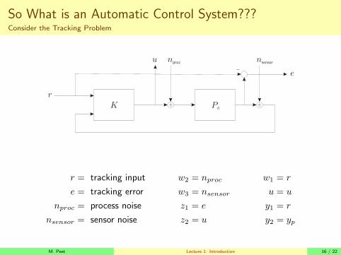
So What is an Automatic Control System???Consider the Tracking Problem12 - 5 LFTs and stability 2001.11.07.04

Example: a tracking problemnproc nsensoru

r

e

P0

K + +

−

y u

P0

P

WsensWact

WprocWerr

K

n wproc 2=

r w= 1

nsensor = w3

z1 = e

z u2 =

++

−r = tracking input w2 = nproc w1 = r

e = tracking error w3 = nsensor u = u

nproc = process noise z1 = e y1 = r

nsensor = sensor noise z2 = u y2 = yp

M. Peet Lecture 1: Introduction 16 / 22

Tracking Control

12 - 5 LFTs and stability 2001.11.07.04

Example: a tracking problemnproc nsensoru

r

e

P0

K + +

−

y u

P0

P

WsensWact

WprocWerr

K

n wproc 2=

r w= 1

nsensor = w3

z1 = e

z u2 =

++

−

P =

I −P0 0 −P0

0 0 0 II 0 0 00 P0 I P0

z1 = r − P0(nproc + u)

z2 = u

y1 = r

y2 = w3 + P0(nproc + u)

M. Peet Lecture 1: Introduction 17 / 22

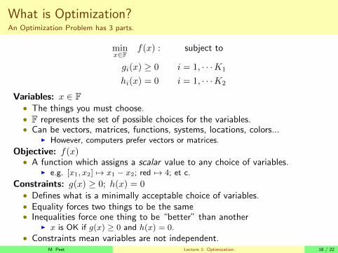
What is Optimization?An Optimization Problem has 3 parts.

minx∈F

f(x) : subject to

gi(x) ≥ 0 i = 1, · · ·K1

hi(x) = 0 i = 1, · · ·K2

Variables: x ∈ F• The things you must choose.• F represents the set of possible choices for the variables.• Can be vectors, matrices, functions, systems, locations, colors...

I However, computers prefer vectors or matrices.

Objective: f(x)• A function which assigns a scalar value to any choice of variables.

I e.g. [x1, x2] 7→ x1 − x2; red 7→ 4; et c.

Constraints: g(x) ≥ 0; h(x) = 0• Defines what is a minimally acceptable choice of variables.• Equality forces two things to be the same• Inequalities force one thing to be “better” than another

I x is OK if g(x) ≥ 0 and h(x) = 0.

• Constraints mean variables are not independent.M. Peet Lecture 1: Optimization 18 / 22

What is Optimization?An Optimization Problem has 3 parts.

minx∈F

f(x) : subject to

gi(x) ≥ 0 i = 1, · · ·K1

hi(x) = 0 i = 1, · · ·K2

Variables: x ∈ F• The things you must choose.• F represents the set of possible choices for the variables.• Can be vectors, matrices, functions, systems, locations, colors...

I However, computers prefer vectors or matrices.

Objective: f(x)• A function which assigns a scalar value to any choice of variables.

I e.g. [x1, x2] 7→ x1 − x2; red 7→ 4; et c.

Constraints: g(x) ≥ 0; h(x) = 0• Defines what is a minimally acceptable choice of variables.• Equality forces two things to be the same• Inequalities force one thing to be “better” than another

I x is OK if g(x) ≥ 0 and h(x) = 0.

• Constraints mean variables are not independent.

2019-08-27

Lecture 1Optimization

What is Optimization?

The word “better” is defined using a notion of positivity (A Complete or PartialOrdering)

EVERYTHING is an Optimization Problem

• Teaching

• Studying

• Choosing a Class

• Getting Lunch

• Getting to Class

• Doing chores

The Trick is Modeling the Optimization Problem

How Hard is it to Solve Optimization Problems

For Humans:

• Almost always IMPOSSIBLE (or at least tedious)

For Computers:

• Easy if the Problem is CONVEX. (Polynomial Time)

• Otherwise IMPOSSIBLE. (NP-Hard)

We will talk about this a bit more later!

M. Peet Lecture 1: Optimization 19 / 22

Now What is an LMI?An LMI is a type of constraint

Definition 2.

A symmetric matrix (P = PT ) is Positive Definite (denoted P > 0) if all of itseigenvalues are positive.

A Linear Matrix Inequality (LMI) is a constraint that looks like

AiPBi +Qi > 0

where P is the variable and Ai, Bi, Qi are matrices.

Question: Why do we have a whole controls course devoted to LMIs?

• LMI constraints are convex (Computers can solve them)

• Positive matrices can be used to study systems.I This is because we are really optimizing Lyapunov functions.I V (x) = xTPx ≥ 0 if P > 0.

Almost ALL computational methods in Control are based on LMIs.

• Or at least be reformulated as an LMI.

M. Peet Lecture 1: Optimization 20 / 22

Now What is an LMI?An LMI is a type of constraint

Definition 2.

A symmetric matrix (P = PT ) is Positive Definite (denoted P > 0) if all of itseigenvalues are positive.

A Linear Matrix Inequality (LMI) is a constraint that looks like

AiPBi +Qi > 0

where P is the variable and Ai, Bi, Qi are matrices.

Question: Why do we have a whole controls course devoted to LMIs?

• LMI constraints are convex (Computers can solve them)

• Positive matrices can be used to study systems.I This is because we are really optimizing Lyapunov functions.I V (x) = xTPx ≥ 0 if P > 0.

Almost ALL computational methods in Control are based on LMIs.

• Or at least be reformulated as an LMI.

2019-08-27

Lecture 1Optimization

Now What is an LMI?

LMIs define a Partial Ordering

• One matrix may not be better or worse than another

• The LMI means the LHS must be better in EVERY way.

Now What is an LMI?An Example: The Lyapunov Inequality

The systemx = Ax

is stable (eigenvalues have negative real part) if and only if there exists a P > 0such that

ATP + PA < 0

YALMIP Code for Stability Analysis:> A = [-1 2 0; -3 -4 1; 0 0 -2];

> P = sdpvar(3,3);

> F = [P >= eye(3)];

> F = [F, A’*P+P*A <= 0];

> optimize(F);

If Feasible, YALMIP Code to Retrieve the Solution:> Pfeasible = value(P);

M. Peet Lecture 1: Optimization 21 / 22

Class Project

In lieu of a final exam, we will have two class projects (Alone or in pairs).1. Write a Wikibook Chapter• Include a minimum of 10 pages (20 for pairs)

2. Do Research/Solve a Problem• Can be based on existing research.

Some Project Ideas:• Gain Scheduling for Missile Attitude Control (Switched Systems)

• Control of Robots over the internet (Sampled-Data Systems)

• Spacecraft Attitude Control with delayed communication (Delay Systems)

• Social Cognitive Therapy using Discrete Inputs (Mixed-Integer Control)

• Self-Driving Vehicles (Decentralized Control)

• Soft Robotics (Decentralized Control)

• Thermostat Programming (Dynamic Programming)

• Flow Control (PDEs)

• Controller/Estimator Design using Arduino and Simulink (Robust Control)

• System Identification using LMIs

• Mobile App for solving an optimization or control problem.

For those who dislike Projects, we can arrange to take a Final Exam instead.M. Peet Lecture 1: Optimization 22 / 22