Formulae of the Full Potential LMTO method: Second Edition (unfinished) S.Yu.Savrasov Department of Physics, New Jersey Institute of Technology, Newark, NJ 07102 (April 2003) Table of Content I. Basic statements. II. Basis functions. a. MT spheres b. Interstitials: Fourier Tranforms of pseudoLMTOs III. Hamiltonian and overlap matrix (MT-part). a. Expressions. b. Radial matrix elements. IV. Hamiltonian (NMT-part within sphere). a. Expressions. b. Matrix elements. V. Hamiltonian and overlap matrix (interstitial region). a. Expressions. b. Matrix elements. VI. Overlap matrix in the interstitial region (derivation through œ S). a. Expressions. b. Derivation. VII. Structure constants and their energy derivatives (Evalds procedure). VIII. Full potential. a. Coulomb part within MT-sphere. b. Coulomb part in the interstitial region. c. Exchange-correlation contribu- tion. IX. Wave functions. a. Denitions. b. Symmetry relations. X. Full density. a. Expressions. b. Numbers of states matrix. c. Core density (Mattheisss procedure). XI. Radial Schr¤ odinger equation. a. Non-relativistic case. b. Scalar-relativistic case. APPENDIX A: Spherical functions. APPENDIX B: Spherical harmonics. APPENDIX C: Spherical coordinates. I. BASIC STATEMENTS It is supposed that the crystalline space is divided into the atom centered spheres and the remaining interstitial region. The charge density and effective potential are expanded in spherical harmonics inside spheres: ρ τ (r τ )= L v τ X L ρ Lτ (r τ )i l Y L ( r) (1) V τ (r τ )= L v τ X L V Lτ (r τ )i l Y L ( r) (2) The Schroedinger equation is solved in terms of the variational principle: (−∇ 2 + V − E kλ )ψ kλ =0 (3) 1
Transcript
Formulae of the Full Potential LMTO method: Second Edition (unfinished)
S.Yu.SavrasovDepartment of Physics, New Jersey Institute of Technology, Newark,
NJ 07102(April 2003)
Table of Content
I. Basic statements.II. Basis functions.a. MT spheresb. Interstitials: Fourier Tranforms of pseudoLMTOsIII. Hamiltonian and overlap matrix (MT-part).a. Expressions. b. Radial matrix elements.IV. Hamiltonian (NMT-part within sphere).a. Expressions. b. Matrix elements.V. Hamiltonian and overlap matrix (interstitial region).a. Expressions. b. Matrix elements.VI. Overlap matrix in the interstitial region (derivation through úS).a. Expressions. b. Derivation.VII. Structure constants and their energy derivatives (Evalds procedure).VIII. Full potential.a. Coulomb part within MT-sphere. b. Coulomb part in the interstitial region. c. Exchange-correlation contribu-
tion.IX. Wave functions.a. DeÞnitions.b. Symmetry relations.X. Full density.a. Expressions.b. Numbers of states matrix.c. Core density (Mattheisss procedure).XI. Radial Schrodinger equation.a. Non-relativistic case.b. Scalar-relativistic case.APPENDIX A: Spherical functions.APPENDIX B: Spherical harmonics.APPENDIX C: Spherical coordinates.
I. BASIC STATEMENTS
It is supposed that the crystalline space is divided into the atom centered spheres and the remaining interstitialregion. The charge density and effective potential are expanded in spherical harmonics inside spheres:
ρτ (rτ ) =
LvτXL
ρLτ (rτ )ilYL(r) (1)
Vτ (rτ ) =
LvτXL
VLτ (rτ )ilYL(r) (2)
The Schroedinger equation is solved in terms of the variational principle:
The space is partitioned into the non overlapping (or slightly overlapping) muffintin spheres sR surrounding everyatom and the remaining interstitial region Ωint. Within the spheres, the basis functions are represented in terms ofnumerical solutions of the radial Schrodinger equation for the spherical part of the potential multiplied by sphericalharmonics as well as their energy derivatives taken at some set of energies .ν at the centers of interest. In theinterstitial region, where the potential is essentially ßat, the basis functions are spherical waves taken as the solutionsof Helmholtzs equation: (−∇2−.)f(r, .) = 0 with some Þxed value of the average kinetic energy . = κ2ν . In particular,in the standard LMTO method using the atomicsphere approximation (ASA), the approximation κ2ν = 0 is chosen.In the extensions of the LMTO method for a potential of arbitrary shape (full potential), a multiplekappa basis setis normally used in order to increase the variational freedom of the basis functions while recent developments of anew LMTO technique promise to avoid this problem.The general strategy for including the fullpotential terms in the calculation is the use of the variational principle.
A few different techniques have been developed for taking the nonspherical corrections into account in the frameworkof the LMTO method. They include Fourier transforms of the LMTOs in the interstitial region, onecenter sphericalharmonics expansions within atomic cells, interpolations in terms of the Hankel functions as well as direct calculationsof the charge density in the tightbinding representation. In two of these schemes the treatment of open structuressuch as, e.g. the diamond structure is complicated and interstitial spheres are usually placed between the atomicspheres. Therefore we will develop the linearresponse LMTO technique using the planewave Fourier representation.We introduce the following partial waves or muffin-tin orbitals deÞned in whole space:
χLκτ (rτ ) =
½ΦHLκτ (rτ ) rτ < SτHLκτ (rτ ) rτ > Sτ
¯(6)
where ΦHLκτ (rτ ) is constructed from the linear combination of φν and úφν with the condition of smooth augmentationat the sphere.
A. MT-Spheres
The LMTO-basis functions are obtained from the Bloch sum of these partial waves:
χkLκτ (r) =
XR
eikRχLκτ (r−R− τ) = ΦHLκτ (rτ )δττ 0 −XR
0eikRHLκτ (r−R− τ) (7)
Using the addition theorem
XR
0eikRHLκτ (r−R− τ) = −
LtτXL0JL0κτ 0(rτ 0)γl0τ 0S
kL0τ 0Lτ (κ) (8)
where SkL0τ 0Lτ (κ) stand for the structure constants and where γlτ =
1Sτ (2l+1)
, we obtain:
χkLκτ (rτ 0) = Φ
HLκτ (rτ )δττ 0 −
LtτXL0JL0κτ 0(rτ 0)γl0τ 0S
kL0τ 0Lτ (κ) (9)
Let us perform the augmentation inside MT-sphere
2
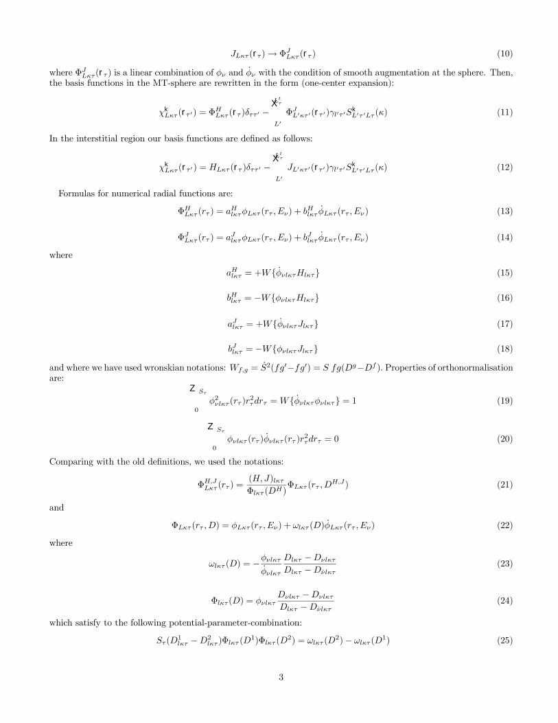
JLκτ (rτ )→ ΦJLκτ (rτ ) (10)
where ΦJLκτ (rτ ) is a linear combination of φν andúφν with the condition of smooth augmentation at the sphere. Then,
the basis functions in the MT-sphere are rewritten in the form (one-center expansion):
χkLκτ (rτ 0) = Φ
HLκτ (rτ )δττ 0 −
LtτXL0ΦJL0κτ 0(rτ 0)γl0τ 0S
kL0τ 0Lτ (κ) (11)
In the interstitial region our basis functions are deÞned as follows:
χkLκτ (rτ 0) = HLκτ (rτ )δττ 0 −
LtτXL0JL0κτ 0(rτ 0)γl0τ 0S
kL0τ 0Lτ (κ) (12)
Formulas for numerical radial functions are:
ΦHLκτ (rτ ) = aHlκτφLκτ (rτ , Eν) + b
HlκτúφLκτ (rτ , Eν) (13)
ΦJLκτ (rτ ) = aJlκτφLκτ (rτ , Eν) + b
JlκτúφLκτ (rτ , Eν) (14)
where
aHlκτ = +W úφνlκτHlκτ (15)
bHlκτ = −WφνlκτHlκτ (16)
aJlκτ = +W úφνlκτJlκτ (17)
bJlκτ = −WφνlκτJlκτ (18)
and where we have used wronskian notations: Wf,g = úS2(fg0−fg0) = S fg(Dg−Df ). Properties of orthonormalisationare: Z Sτ
0
φ2νlκτ (rτ )r2τdrτ =W úφνlκτφνlκτ = 1 (19)
Z Sτ
0
φνlκτ (rτ ) úφνlκτ (rτ )r2τdrτ = 0 (20)
Comparing with the old deÞnitions, we used the notations:
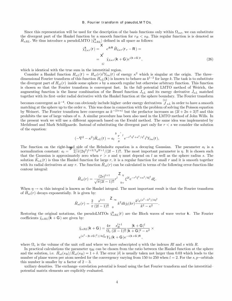
Since this representation will be used for the description of the basis functions only within Ωint, we can substitutethe divergent part of the Hankel function by a smooth function for rR < sR. This regular function is is denoted asHκRL. We thus introduce a pseudoLMTO |χk
κRLi deÞned in all space as follows:χkLκτ (r) =
Xt
eikR HLκτ (rτ −R) =
=XG
χLκτ (k+G)ei(k+G)r, (26)
which is identical with the true sum in the interstitial region.Consider a Hankel function HκL(r) = Hκl(r)i
lYlm(r) of energy κ2 which is singular at the origin. The three
dimensional Fourier transform of this function HκL(k) is known to behave as kl−2 for large k.The task is to substitutethe divergent part of Hκl(r) inside some sphere s by a smooth regular but otherwise arbitrary function. This functionis chosen so that the Fourier transform is convergent fast. In the fullpotential LMTO method of Weirich, theaugmenting function is the linear combination of the Bessel function JκL and its energy derivative úJκL matchedtogether with its Þrstorder radial derivative with the Hankel function at the sphere boundary. The Fourier transform
becomes convergent as k−4. One can obviously include higherorder energy derivatives(n)
J κL in order to have a smoothmatching at the sphere up to the order n. This was done in connection with the problem of solving the Poisson equationby Weinert. The Fourier transform here converges as k−(3+n) but the prefactor increases as (2l + 2n+ 3)!! and thisprohibits the use of large values of n. A similar procedure has been also used in the LMTO method of John Wills. Inthe present work we will use a different approach based on the Ewald method. The same idea was implemented byMethfessel and Mark Schilfgaarde. Instead of substituting the divergent part only for r < s we consider the solutionof the equation:
(−∇2 − κ2) HκL(r) = al³rs
´le−r
2η2+κ2/η2
ilYlm(r),
The function on the right-hand side of the Helmholtz equation is a decaying Gaussian. The parameter al is anormalization constant: al =
p2/π(2η2)l+3/2s2l+1/(2l − 1)!!. The most important parameter is η. It is chosen such
that the Gaussian is approximately zero when r > s and η must depend on l as well as the sphere radius s. Thesolution KκL(r) is thus the Hankel function for large r, it is a regular function for small r and it is smooth together
with its radial derivatives at any r. The function Hκl(r) can be calculated in terms of the following error-function-likecontour integral:
Hκl(r) =(2s)l+1√π(2l − 1)!!r
l
Z η
0+
ξ2le−r2ξ2+κ2/4ξ2
dξ.
When η →∞ this integral is known as the Hankel integral. The most important result is that the Fourier transformof Hκl(r) decays exponentially. It is given by:
Hκl(r) =2
π
sl+1
(2l− 1)!!Z ∞
0
k2dkjl(kr)kle(κ
2−k2)/4η2
k2 − κ2 .
Restoring the original notations, the pseudoLMTOs χkκRL(r) are the Bloch waves of wave vector k. The Fourier
coefficients χκRL(k+G) are given by:
χκRL(k+G) =4π
Ωc
sl+1R
(2l − 1)!!|k+G|l
|k+G|2 − κ2 ×
e(κ2−|k+G|2)/4η2
RlYL(k+G)e−i(k+G)R,
where Ωc is the volume of the unit cell and where we have subscripted η with the indexes Rl and s with R.In practical calculations the parameter ηRl can be chosen from the ratio between the Hankel function at the sphere
and the solution, i.e. Hκl(sR)/ Hκl(sR) = 1+ δ. The error |δ| is usually taken not larger than 0.03 which leads to thenumber of plane waves per atom needed for the convergency varying from 150 to 250 when l = 2. For the s, p−orbitalsthis number is smaller by a factor of 2− 3.uxiliary densities. The exchangecorrelation potential is found using the fast Fourier transform and the interstitial
potential matrix elements are explicitly evaluated.
4
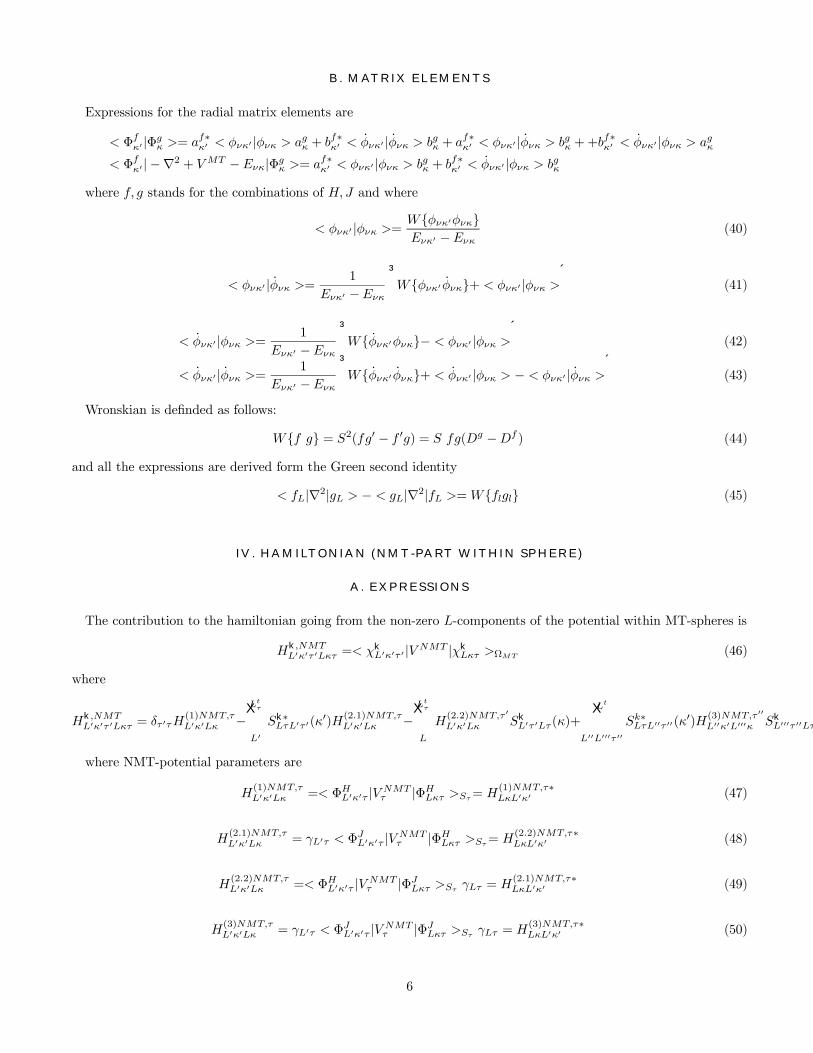
III. HAMILTONIAN AND OVERLAP MATRIX (MT-PART)
The hamiltonian and overlap matrices are separated into the following contributions:
HkL0κ0τ 0Lκτ = H
k,MTL0κ0τ 0Lκτ +H
k,NMTL0κ0τ 0Lκτ + κ
2Ok,INTL0κ0τ 0Lκτ + V
k,INTL0κ0τ 0Lκτ
OkL0κ0τ 0Lκτ = O
k,MTL0κ0τ 0Lκτ +O
k,INTL0κ0τ 0Lκτ
where the Þrst term in H-matrix represents the contribution of the MT-part of the one-electron hamiltonian andthe second term is the non-muffin-tin correction within MT-space. The third term is the matrix element of kineticeenergy in the interstitial region and the fourth term is the interstitial-potential matrix element. The O-matrix is alsodivided to the contributions from inside the spheres and from the interstitials. We Þrst study the MT-part of thesematrices.
A. EXPRESSIONS
The MT-part of the hamiltonian and overlap matrix is deÞned as follows:
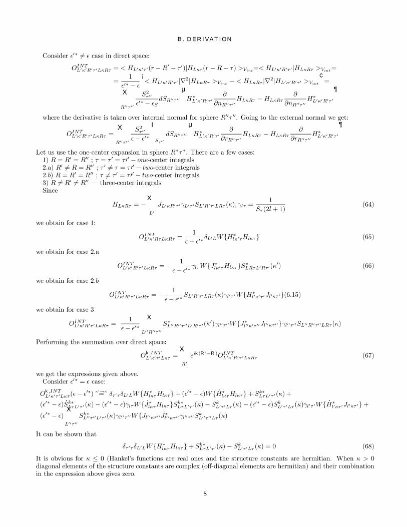
It is obvious for κ ≤ 0 (Hankels functions are real ones and the structure constants are hermitian. When κ > 0diagonal elements of the structure constants are complex (off-diagonal elements are hermitian) and their combinationin the expression above gives zero.
8
VI. STRUCTURE CONSTANTS AND THEIR ENERGY DERIVATIVES
LMTO-structure constants are given by
SkL0τ 0Lτ (κ) = (Sτ 0Sτ )
1/2Xl00gl
00L0L(κSWZ)
l+l0−l00µSτ 0
SWZ
¶l0+1/2 µSτSWZ
¶l+1/2×Σk
l00m0−m,τ 0−τ (E)
where
gl00L0L = −
8π√4π
(2l00 − 1)!!(2l0 − 1)!!(2l − 1)!!C
L00LL0 (69)
and the lattice sum is given by:
ΣkLδ(.) =
X0ReikRHlκWZ(|R− δ|)[
√4πilYL( R− δ)]∗ (70)
Evalds transformation for the lattice sum is:
ΣkLδ(.) = Σ
k(1)Lδ (.) +Σ
k(2)Lδ (.) +Σ
(3)Lδ (.) (71)
where
Σk(1)Lδ (.) =
8π√π
(2l − 1)!!Sl+1WZ
Ωce>/4η
2 XG
|k+G|le−|k+G|2/4η2
|k+G|2 − . ei(k+G)δY ∗L (k+G)
Σk(2)Lδ (.) =
4(−2i)l+1(2l − 1)!! S
l+1WZ
0XR
eikR|R− δ|lY ∗L (R−δ)Z ∞
η
dξ ξ2le−|R−δ|2ξ2+>/4ξ2
Σ(3)Lδ (.) = δL0δδ0
2ηSWZ√π
∞Xn=0
(./4η2)n
n!(2n− 1) − δL0δδ0iSWZ
√.(7.7)
and κ2 = . while . can be considered in units (1/a)2.Energy derivatives of the LMTO-structure constants are given by
úSkL0τ 0Lτ (κ) = S
2WZ
d
d.SkL0τ 0Lτ (κ) = S
2WZ
³úS
k(1)L0τ 0Lτ (κ) +
úSk(2)L0τ 0Lτ (κ)
´where we deÞne:
úSk(1)L0τ 0Lτ (κ) =
1
2(Sτ 0Sτ )
1/2Xl00gl
00L0L(l + l
0 − l00)12(κSWZ)
l+l0−l00µSτ 0
SWZ
¶l0+1/2 µSτSWZ
¶l+1/2×
Σkl00m0−m,τ 0−τ (.) (72)
úSk(2)L0τ 0Lτ (κ) =
Xl00gl
00L0L(κSWZ)
l+l0−lµ
Sτ 0
SWZ
¶l0+1/2 µSτSWZ
¶l+1/2× úΣk
l00m0−m,τ 0−τ (.)
and where the energy derivative of the lattice sum is:
úΣkLδ(.) =
0XR
eikR úHlκWZ(|R− δ|)[√4πilYL(R−δ)]∗ (73)
Evalds transformation for the lattice sum is:
9
úΣkLδ(.) = úΣ
k(1)Lδ (.) +
úΣk(2)Lδ (.) +
úΣ(3)Lδ (.) (74)
where
úΣk(1)Lδ (.) =
8π√πSl−1WZ
(2l − 1)!!Ωce>/4η
2 XG
|k+G|le−|k+G|2/4η2
|k+G|2 − . ei(k+G)δY ∗L(k+G)
µ1
4η2+
1
|k+G|2 − .
úΣk(2)Lδ (.) =
4(−2i)l+1(2l− 1)!! S
l−1WZ
0XR
eikR|R− δ|lY ∗L(R−δ)1
4
Z ∞
η
dξ ξ2l−2e−|R−δ|2ξ2+>/4ξ2
úΣ(3)Lδ (.) = δL0δδ0
1
2√πηSW Z
∞Xn=0
(./4η2)n
n!(2n+ 1)− δL0δδ0 i
2SWZ√.
Error function integrals are given by:
Fl(η,∆, .) =
Z ∞
η
dξ ξ2le−∆2ξ2+>/4ξ2
(75)
and satisfy to the following recurrent relationships:
2∆2Fl+1(η,∆, .) = e−∆2η2+>/4η2
η2l+1 + (2l + 1)Fl(η,∆, .)− .
2Fl−1(η,∆, .) (76)
First integrals are:
F0(η,∆, .) =e−∆
2η2
2∆
Z ∞
0
dx
(x+∆2η2)1/2e−x exp(
.∆2
4(x+∆2η2)) (77)
F−1(η,∆, .) =∆
2e−∆
2η2
Z ∞
0
dx
(x+∆2η2)3/2e−x exp(
.∆2
4(x+∆2η2)) (78)
which have been reduced to Gauss-Laguerre quadrature integration.Note that for . = 0 the last contribution to úΣ(3) diverges. It must be dropped since it is cancelled out with the
same divergency in wronskian WHκ úHκ0 when .missmiss0. Note also that for . > 0, S and S − dot matrices arenot hermitian since Hankels functions are complex. This non-hermitianness goes from the last contribution to Σ(3)
and, consequently, diagonal elements of S and S−dot are complex numbers. This last contribution to Σ(3) is, indeed,equal to the lattice sum of Bessels functions. By considering Neumans functions for E > 0 we can, in priniple, obtainhermitian structure constants.Usefull properties of Σ-constants in case real energies:
Σklm,−δ(.) = (−1)mΣk∗l−m,δ(.) (79)
úΣklm,−δ(.) = (−1)m úΣk∗l−m,δ(.) (80)
In case k = 0, . = 0 the divergent contribution with G = 0 in Σ(1)l=0 must be dropped from the electroneutrality
condition. Instead, Σ(4)l=0 contribution is appeared which is given by
Σ(4)Lδ (. = 0) = δL0
−34Natomη2S2WZ
(81)
It can be shown that the singularities appeared in Σ-constants when .missmiss0 and kmissmiss0 are also cancelledout if one assumes the absence of dipol and quadrupole moments of the whole crystal. This is valid if one Þrst sets. = 0 and then k → 0. If one sets k = 0 and then considers the limit .→0 one more term seems to appear:
Sk=0L0τ 0Lτ (. = 0) =??? + δl01δl1δm0m8π√π
ΩcellS2τ 0S
2τ/√4π(7.24)
In this case, only electroneutrality condition can be assumed to get this limit behavior.
10
More useful relations:
S−kL0τ 0Lτ (.) = (−)l0+m0+l+mSkLτL0τ 0(.) (82)
for any . (7.25)
Sk∗L0τ 0Lτ (.) = SkLτL0τ 0(.) (83)
for real energies (7.26)
S−k∗L0τ 0Lτ (.) = (−)l0+m0+l+mSkL0τ 0Lτ (.) (84)
VII. FULL POTENTIAL
A. COULOMB PART WITHIN MT-SPHERE
Electrostatic potential inside MT-sphere is given by
V Cτ (rτ ) = −δL0Zτe
2
rτ
√4πY00 + e
2XL
µrτSτ
¶lilYL(rτ )
4π
2l + 1Slτ
Z Sτ
rτ
ρLτ (r0τ )r
0−l−1τ r02τdr
0τ +
+e2XL
µSτrτ
¶+l+1ilYL(rτ )
4π
2l + 1S−l−1τ
Z rτ
0
ρLτ (r0τ )r
0lτr02τdr
0τ +
e2XL
µrτSτ
¶lilYL(rτ )
hQ(1)Lτ +Q
(2)Lτ
iwhere
Q(1)Lτ =
√4π
Sτ (2l + 1)t(1)Lτ (85)
Q(2)Lτ = −
√4π
Sτ (2l + 1)
XL0τ 0
Sk=0LτL0τ 0(κ = 0)MtotL0τ 0
Sτ 0(2l0 + 1)(86)
MtotLτ = −ZτδL0 +Mρ
Lτ + t(2)Lτ (87)
MρLτ =
√4πS−lτ
Z Sτ
0
ρLτ (rτ )rlτr2τdrτ (88)
t(1)Lτ =
√4πSl+1τ
ZΩiτ
tcolρnτt(rτ )[r
−l−1τ ilYL(rτ )]
∗drτ (89)
t(2)Lτ =
√4πS−lτ
ZΩiτ
tcolρnτt(rτ )[r
lτ ilYL(rτ )]
∗drτ (90)
Integrals over intersitital region are given by:
t(1)Lτ =
√4πSl+1τL
2LwτX0n0n
Aρ,n0
L0τ A(1),nl τ
XL
CLLL0il0−lTn
0nLτ = (91)
√4πSl+1τ
Xn
A(1),nl τ Cρ,nLτ t
(2)Lτ =
√4πS−lτL
2LwτX0n0n
Aρ,n0
L0τ A(2),nl τ
XL
CLLL0il0−lTn
0nLτ =
√4πS−lτ
Xn
A(2),nl τ Cρ,nLτ (92)
11
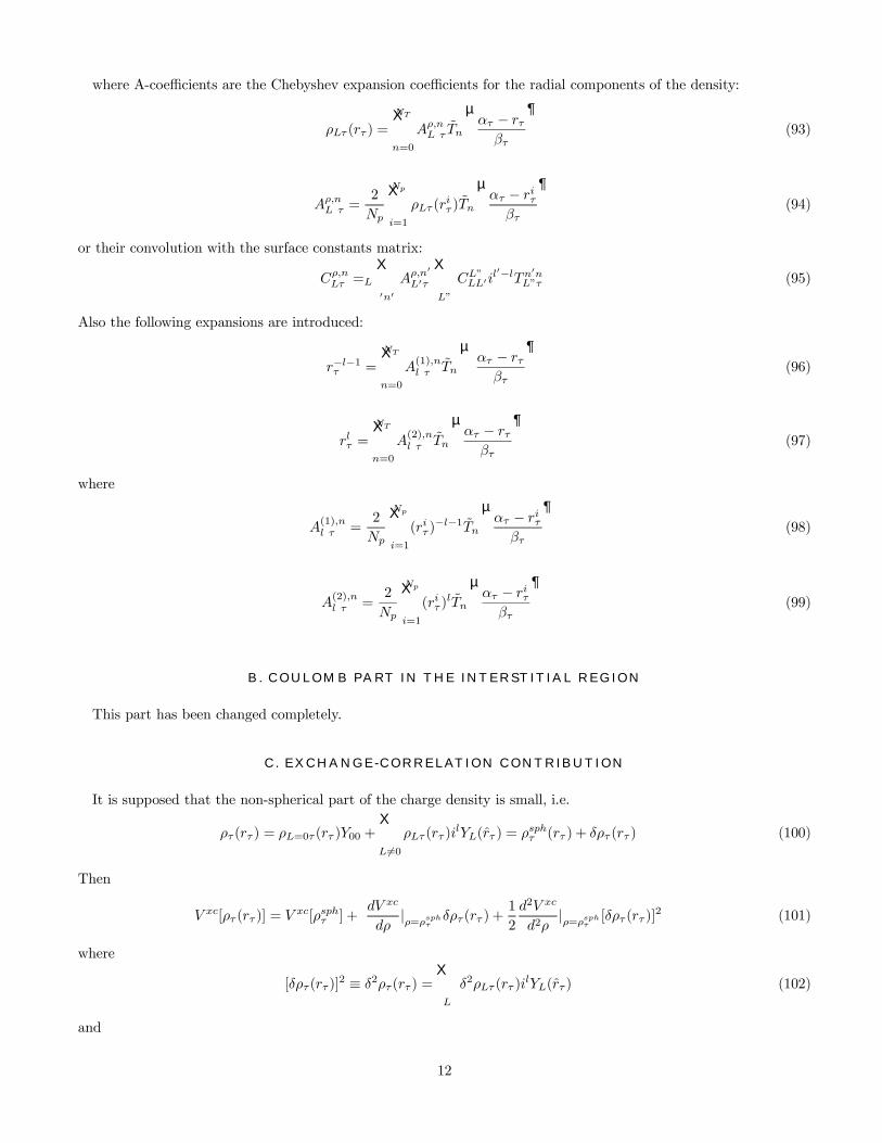
where A-coefficients are the Chebyshev expansion coefficients for the radial components of the density:
ρLτ (rτ ) =NTXn=0
Aρ,nL τTn
µατ − rτβτ
¶(93)
Aρ,nL τ =2
Np
NpXi=1
ρLτ (riτ ) Tn
µατ − riτβτ
¶(94)
or their convolution with the surface constants matrix:
Cρ,nLτ =LX0n0Aρ,n
0L0τ
XL
CLLL0il0−lTn
0nLτ (95)
Also the following expansions are introduced:
r−l−1τ =
NTXn=0
A(1),nl τ
Tn
µατ − rτβτ
¶(96)
rlτ =NTXn=0
A(2),nl τ
Tn
µατ − rτβτ
¶(97)
where
A(1),nl τ =
2
Np
NpXi=1
(riτ )−l−1 Tn
µατ − riτβτ
¶(98)
A(2),nl τ =
2
Np
NpXi=1
(riτ )l Tn
µατ − riτβτ
¶(99)
B. COULOMB PART IN THE INTERSTITIAL REGION
This part has been changed completely.
C. EXCHANGE-CORRELATION CONTRIBUTION
It is supposed that the non-spherical part of the charge density is small, i.e.
ρτ (rτ ) = ρL=0τ (rτ )Y00 +XL6=0
ρLτ (rτ )ilYL(rτ ) = ρ
sphτ (rτ ) + δρτ (rτ ) (100)
Then
V xc[ρτ (rτ )] = Vxc[ρsphτ ] +
dV xc
dρ|ρ=ρsphτ
δρτ (rτ ) +1
2
d2V xc
d2ρ|ρ=ρsphτ
[δρτ (rτ )]2 (101)
where
[δρτ (rτ )]2 ≡ δ2ρτ (rτ ) =
XL
δ2ρLτ (rτ )ilYL(rτ ) (102)
and
12
δ2ρL00τ (rτ ) =LX0L6=0
il+l0−l00ρLτ (rτ )CL
0LL00ρL0τ (rτ ) (103)
Radial derivatives are given by
δ2ρ0L(rτ ) =LX0L6=0
2il+l0−lρ0
Lτ (rτ )CL0LLmiss
ρL0τ (rτ ) (104)
δ2ρ0L0miss
τ(rτ ) =LX0L6=0
2il+l0−lρ0Lτ (rτ )C
L0LLρ
0L0τ (rτ ) +L
X0L6=0
il+l0−lρ0L0τ (rτ )C
L0LLρL0τ (rτ )
and spherical part is given by
δ2ρL=0τ (rτ ) =1√4π
XL6=0
(−1)lρlmτ (rτ )ρl−mτ (rτ ) (105)
With the above deÞnitions the exchange-correlation part to the potential is
V xcτ (rτ ) =XL
V xcLτ (rτ )ilYL(rτ ) (106)
V xcLτ (rτ ) =√4πV xc[ρsphτ ]δL0 + µ
xc[ρsphτ ]ρLτ (1− δL0) + 1
2ηxc[ρsphτ ]δ2ρLτ (rτ ) (107)
where the following notations have been used
µxc =dV xc
dρ; ηxc =
d2V xc
d2ρ; γxc =
d3V xc
d3ρ(108)
for different derivatives of local-density-approximation-formulas.
VIII. WAVE FUNCTIONS
A. DEFINITIONS
The wave function is given as the expansion over LMTOs:
ψkλ(r) =
LvτXLκτ
AkλLκτχ
kLκτ (r) (109)
Inside MT-sphere it is represented as the one-center expansion:
ψkλ(rτ ) =XLκ
AkλLκτΦ
HLκτ (rτ )−
XLκ
SkλLκτγlτΦ
JLκτ (rτ ) (110)
and in the interstitial region the wave function has the same form:
ψkλ(rτ ) =XLκ
AkλLκτHLκτ (rτ )−
XLκ
SkλLκτγlτJLκτ (rτ ) (111)
where AkλLκτ are the variational coefficients of the LMTO-eigenvalue problem and SkλLκτ are their convolution with thestructure constants, i.e
SkλLκτ =
XL0τ 0
SkLτL0τ 0(κ)A
kλL0κτ 0 (112)
13
B. SYMMETRY RELATIONS
Let us consider group operations transforming wave functions. If g is an operator of a space group it can be givenby rotation γ and shift a, i.e.
g = γ|a (113)
g−1 = γ−1|− γ−1a (114)
gp = γ|aξ|b = γ ξ|γb+ a (115)
such that
gr = γr + a (116)
g−1r = γ−1r − γ−1a (117)
After applying a point group operation γ coefficients AkλLκτ are transformed in terms of Wigners matrices:
Aγklmκτ =
Xm0U lmm0(γ)Akλ
lm0κg−1τeikRg (118)
Rg = g−1τ − [g−1τ ]inp (119)
where vector in brackets refers to an input basis vector. It can be readily proved that the coefficients S are transformedin the same manner if we account for the tranformation for LMTO-structure constants:
Sγkl0m0τ 0lmτ (κ) =
Xm1m2
U l0m0m1
(γ)Skl0m1g−1τ 0lm2g−1τ (κ)U
l∗mm2
(γ)eik(R0g−Rg) (120)
where
Rg = g−1τ − [g−1τ ]inp (121)
R0g = g
−1τ 0 − [g−1τ 0]inp (122)
IX. FULL DENSITY
A. EXPRESSIONS
The full charge density inside MT-sphere is given by:
ρτ (rτ ) =Xkλ
2fkλψ∗kλ(rτ )ψkλ(rτ ) = (123)X
kλ
2fkλ
XL0κ0L κ
Akλ∗L0κ0τA
kλLκτΦ
H∗L0κ0τ (rτ )Φ
HLκτ (rτ )−
Xkλ
2fkλ
XL0κ0L κ
Akλ∗L0κ0τS
kλLκτΦ
H∗L0κ0τ (rτ )Φ
JLκτ (rτ )γlτ − (124)
Xkλ
2fkλ
XL0κ0L κ
Skλ∗L0κ0τA
kλLκτγl0τΦ
J∗L0κ0τ (rτ )Φ
HLκτ (rτ ) +
Xkλ
2fkλ
XL0κ0L κ
Skλ∗L0κ0τS
kλLκτγl0τΦ
J∗L0κ0τ (rτ )Φ
JLκτ (rτ )γlτ (125)
or as an expansion in spherical harmonics
ρτ (rτ ) =
LvτXL00ρL00τ (rτ )i
l00YL00(rτ ) (126)
14
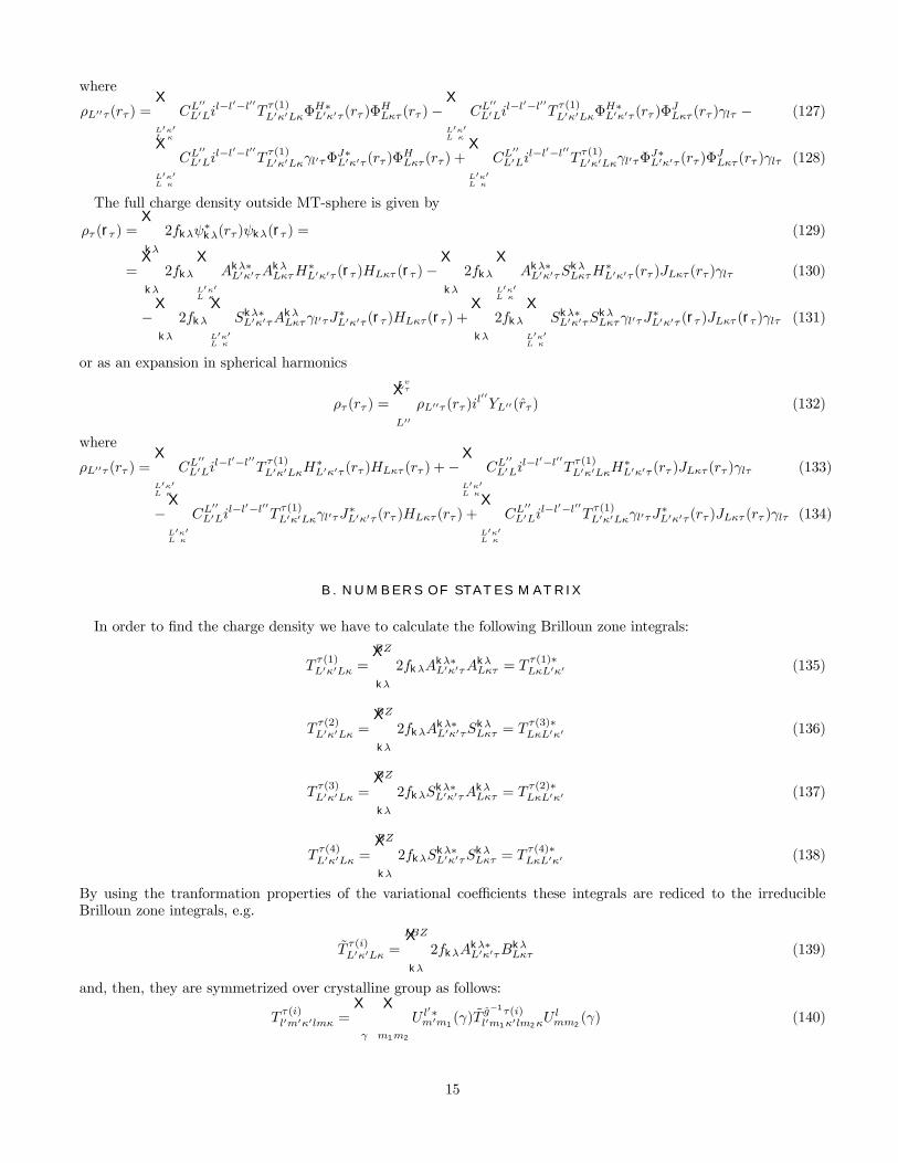
where
ρL00τ (rτ ) =XL0κ0L κ
CL00
L0Lil−l0−l00T τ(1)L0κ0LκΦ
H∗L0κ0τ (rτ )Φ
HLκτ (rτ )−
XL0κ0L κ
CL00
L0Lil−l0−l00T τ(1)L0κ0LκΦ
H∗L0κ0τ (rτ )Φ
JLκτ (rτ )γlτ − (127)
XL0κ0L κ
CL00
L0Lil−l0−l00T τ(1)L0κ0Lκγl0τΦ
J∗L0κ0τ (rτ )Φ
HLκτ (rτ ) +
XL0κ0L κ
CL00
L0Lil−l0−l00T τ(1)L0κ0Lκγl0τΦ
J∗L0κ0τ (rτ )Φ
JLκτ (rτ )γlτ (128)
The full charge density outside MT-sphere is given by
ρτ (rτ ) =Xkλ
2fkλψ∗kλ(rτ )ψkλ(rτ ) = (129)
=Xkλ
2fkλ
XL0κ0L κ
Akλ∗L0κ0τA
kλLκτH
∗L0κ0τ (rτ )HLκτ (rτ )−
Xkλ
2fkλ
XL0κ0L κ
Akλ∗L0κ0τS
kλLκτH
∗L0κ0τ (rτ )JLκτ (rτ )γlτ (130)
−Xkλ
2fkλ
XL0κ0L κ
Skλ∗L0κ0τA
kλLκτγl0τJ
∗L0κ0τ (rτ )HLκτ (rτ ) +
Xkλ
2fkλ
XL0κ0L κ
Skλ∗L0κ0τS
kλLκτγl0τJ
∗L0κ0τ (rτ )JLκτ (rτ )γlτ (131)
or as an expansion in spherical harmonics
ρτ (rτ ) =
LvτXL00ρL00τ (rτ )i
l00YL00(rτ ) (132)
where
ρL00τ (rτ ) =XL0κ0L κ
CL00
L0Lil−l0−l00T τ(1)L0κ0LκH
∗L0κ0τ (rτ )HLκτ (rτ ) +−
XL0κ0L κ
CL00
L0Lil−l0−l00T τ(1)L0κ0LκH
∗L0κ0τ (rτ )JLκτ (rτ )γlτ (133)
−XL0κ0L κ
CL00
L0Lil−l0−l00T τ(1)L0κ0Lκγl0τJ
∗L0κ0τ (rτ )HLκτ (rτ ) +
XL0κ0L κ
CL00
L0Lil−l0−l00T τ(1)L0κ0Lκγl0τJ
∗L0κ0τ (rτ )JLκτ (rτ )γlτ (134)
B. NUMBERS OF STATES MATRIX
In order to Þnd the charge density we have to calculate the following Brilloun zone integrals:
Tτ(1)L0κ0Lκ =
BZXkλ
2fkλAkλ∗L0κ0τA
kλLκτ = T
τ(1)∗LκL0κ0 (135)
Tτ(2)L0κ0Lκ =
BZXkλ
2fkλAkλ∗L0κ0τS
kλLκτ = T
τ(3)∗LκL0κ0 (136)
Tτ(3)L0κ0Lκ =
BZXkλ
2fkλSkλ∗L0κ0τA
kλLκτ = T
τ(2)∗LκL0κ0 (137)
Tτ(4)L0κ0Lκ =
BZXkλ
2fkλSkλ∗L0κ0τS
kλLκτ = T
τ(4)∗LκL0κ0 (138)
By using the tranformation properties of the variational coefficients these integrals are rediced to the irreducibleBrilloun zone integrals, e.g.
Tτ(i)L0κ0Lκ =
IBZXkλ
2fkλAkλ∗L0κ0τB
kλLκτ (139)
and, then, they are symmetrized over crystalline group as follows:
Tτ(i)l0m0κ0lmκ =
Xγ
Xm1m2
U l0∗m0m1
(γ) Tg−1τ(i)l0m1κ0lm2κ
U lmm2(γ) (140)
15
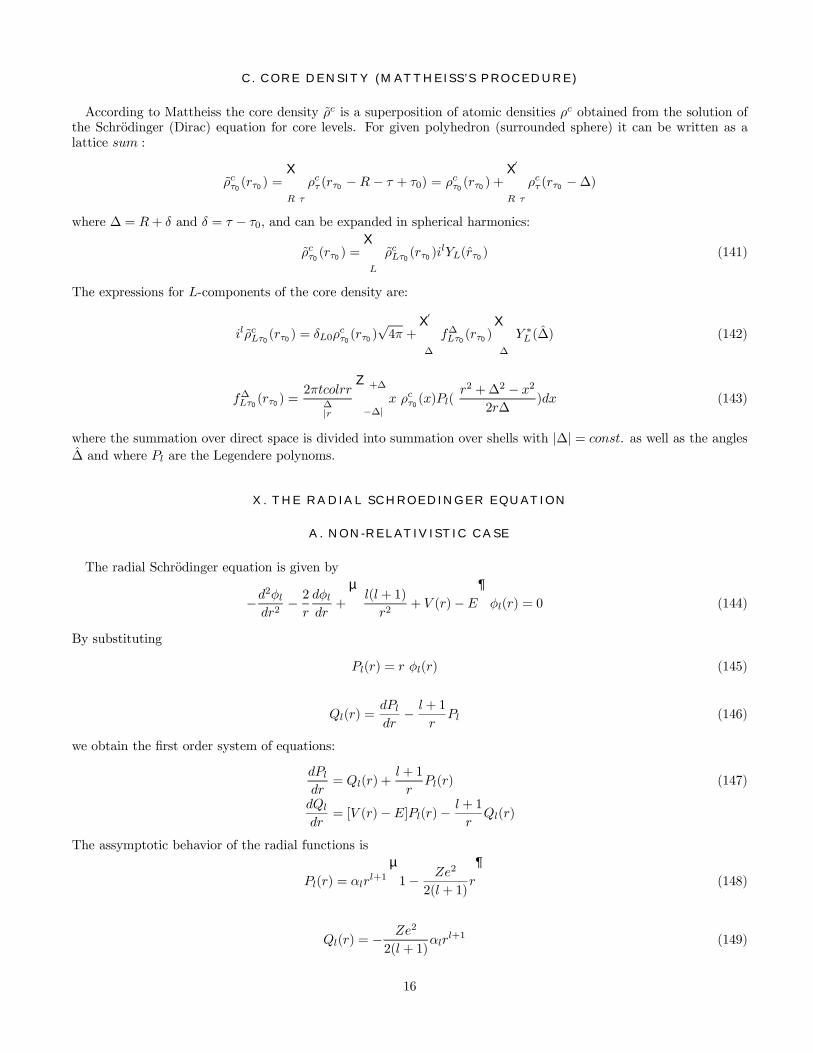
C. CORE DENSITY (MATTHEISS’S PROCEDURE)
According to Mattheiss the core density ρc is a superposition of atomic densities ρc obtained from the solution ofthe Schrodinger (Dirac) equation for core levels. For given polyhedron (surrounded sphere) it can be written as alattice sum :
ρcτ0(rτ0) =
XR τ
ρcτ (rτ0 −R − τ + τ0) = ρcτ0(rτ0) +
0XR τ
ρcτ (rτ0 −∆)
where ∆ = R+ δ and δ = τ − τ0, and can be expanded in spherical harmonics:
ρcτ0(rτ0) =
XL
ρcLτ0(rτ0)i
lYL(rτ0) (141)
The expressions for L-components of the core density are:
ilρcLτ0(rτ0) = δL0ρ
cτ0(rτ0)
√4π +
0X∆
f∆Lτ0(rτ0)
X∆
Y ∗L ( ∆) (142)
f∆Lτ0(rτ0) =
2πtcolrr∆|r
Z +∆
−∆|x ρcτ0
(x)Pl(r2 +∆2 − x2
2r∆)dx (143)
where the summation over direct space is divided into summation over shells with |∆| = const. as well as the angles∆ and where Pl are the Legendere polynoms.
X. THE RADIAL SCHROEDINGER EQUATION
A. NON-RELATIVISTIC CASE
The radial Schrodinger equation is given by
−d2φldr2
− 2r
dφldr
+
µl(l + 1)
r2+ V (r)−E
¶φl(r) = 0 (144)
By substituting
Pl(r) = r φl(r) (145)
Ql(r) =dPldr
− l + 1rPl (146)
we obtain the Þrst order system of equations:
dPldr
= Ql(r) +l + 1
rPl(r) (147)
dQldr
= [V (r)−E]Pl(r)− l + 1rQl(r)
The assymptotic behavior of the radial functions is
Pl(r) = αlrl+1
µ1− Ze2
2(l + 1)r
¶(148)
Ql(r) = − Ze2
2(l + 1)αlr
l+1 (149)
16
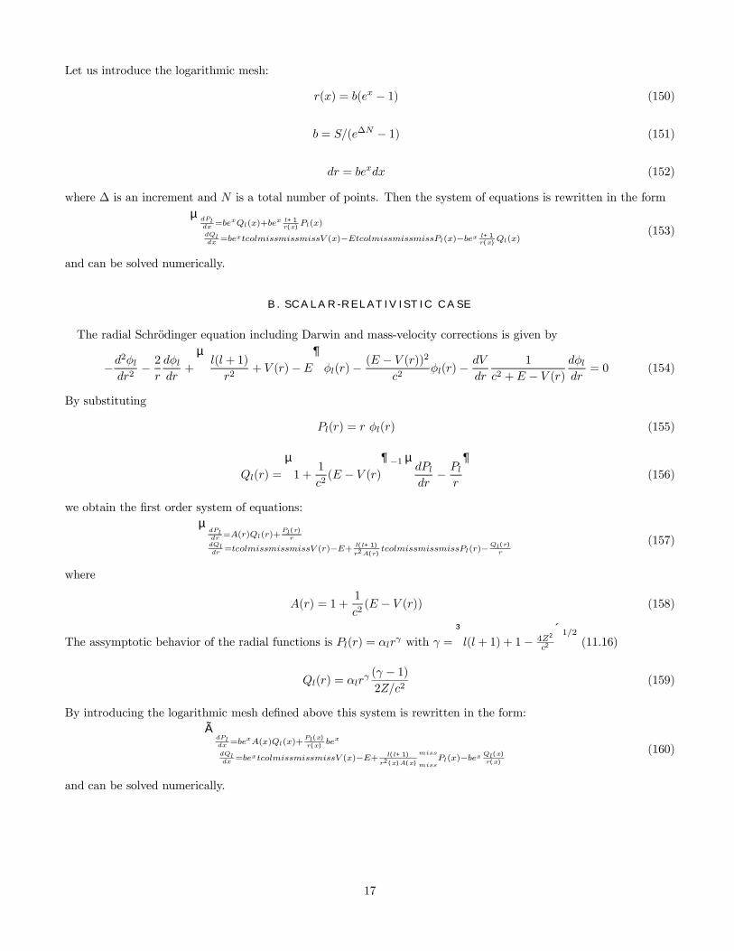
Let us introduce the logarithmic mesh:
r(x) = b(ex − 1) (150)
b = S/(e∆N − 1) (151)
dr = bexdx (152)
where ∆ is an increment and N is a total number of points. Then the system of equations is rewritten in the formµdPldx =be
The radial Schrodinger equation including Darwin and mass-velocity corrections is given by
−d2φldr2
− 2r
dφldr
+
µl(l + 1)
r2+ V (r)−E
¶φl(r)− (E − V (r))
2
c2φl(r)− dV
dr
1
c2 +E − V (r)dφldr
= 0 (154)
By substituting
Pl(r) = r φl(r) (155)
Ql(r) =
µ1+
1
c2(E − V (r)
¶−1 µdPldr
− Plr
¶(156)
we obtain the Þrst order system of equations:µdPldr =A(r)Ql(r)+
Pl(r)
rdQldr =tcolmissmissmissV (r)−E+ l(l+1)
r2A(r)tcolmissmissmissPl(r)−Ql(r)
r
(157)
where
A(r) = 1+1
c2(E − V (r)) (158)
The assymptotic behavior of the radial functions is Pl(r) = αlrγ with γ =
³l(l + 1) + 1− 4Z2
c2
´1/2(11.16)
Ql(r) = αlrγ (γ − 1)2Z/c2
(159)
By introducing the logarithmic mesh deÞned above this system is rewritten in the form:ÃdPldx =be
xA(x)Ql(x)+Pl(x)
r(x)bex
dQldx =be
xtcolmissmissmissV (x)−E+ l(l+1)
r2(x)A(x)
miss
missPl(x)−bex Ql(x)
r(x)
(160)
and can be solved numerically.
17
XI. APPENDIX: SPHERICAL FUNCTIONS
Spherical functions used here are deÞned as follows:
Jlκ(r) =(2l + 1)!!
(κS)ljl(κr)=>
³ rS
´l µ1− (κr)2
2(2l + 3)+ ...
¶(A.1)
Nlκ(r) = − (κS)l+1
(2l − 1)!!nl(κr)=>³ rS
´−l−1 µ1+
(κr)2
2(2l − 1) + ...¶(A.2)
Hlκ(r) = − (κS)l+1
(2l − 1)!!hl(κr)=>³ rS
´−l−1 µ1+
(κr)2
2(2l − 1) + ...¶(A.3)
where jl, nl are the spherical Bessel and Neuman functions and hl = nl − i jl are the Hankel functions.Recurrent relations including radial derivatives:
dJlκ(r)
dr= − l + 1
rJlκ(r) +
(2l + 1)
SJl−1κ(r) ; ∀E (161)
dJlκ(r)
dr=l
rJlκ(r) +
(|κ|S)2S
1
(2l + 3)Jl+1κ(r);E < 0 (162)
dJlκ(r)
dr=l
rJlκ(r)− (κS)2
S
1
(2l + 3)Jl+1κ(r);E > 0 (163)
dHlκ(r)
dr= − l + 1
rHlκ(r)− (|κ|S)
2
S
1
(2l − 1)Hl−1κ(r);E < 0) (164)
dHlκ(r)
dr= − l + 1
rHlκ(r) +
(κS)2
S
1
(2l− 1)Hl−1κ(r);E > 0 (165)
dHlκ(r)
dr=l
rHlκ(r)− (2l + 1)
SHl+1κ(r);∀E (166)
Recurrent relations
Jl+1κ(r) =(2l + 1)(2l + 3)
(|κ|S)2³Jl−1κ(r)− r
SJlκ(r)
´;E < 0 (167)
Jl+1κ(r) = −(2l + 1)(2l+ 3)(κS)2
³Jl−1κ(r)− r
SJlκ(r)
´;E > 0 (168)
Hl+1κ(r) =S
rHlκ(r) +
(|κ|S)2(2l− 1)(2l + 1)Hl−1κ(r);E < 0 (169)
Hl+1κ(r) =S
rHlκ(r)− (κS)2
(2l− 1)(2l + 1)Hl−1κ(r);E > 0 (170)
Relations including second order derivatives
18
d2Jlκ(r)
d2r=
µl(l + 1)
r2−E
¶Jlκ(r)− 2
r
dJlκ(r)
dr;∀E (171)
d2Hlκ(r)
d2r=
µl(l + 1)
r2−E
¶Hlκ(r)− 2
r
dHlκ(r)
dr;∀E (172)
Relations including energy derivatives
dJlκ(r)
dE= úJlκ(r) =
r
2E
µdJlκ(r)
dr− l
rJlκ(r)
¶= − rS
2(2l + 3)Jl+1κ(r);∀E(A.17)
dHlκ(r)
dE= úHlκ(r) =
r
2E
µdHlκ(r)
dr+l + 1
rJlκ(r)
¶=
rS
2(2l − 1)Hl−1κ(r);∀E(A.18)
d úJlκ(r)
dr= úJ 0lκ(r) = −
S
2(2l + 3)Jl+1κ(r)− rS
2(2l + 3)J 0l+1κ(r);∀E(A.19)
d úHlκ(r)
dr= úH 0
lκ(r) =S
2(2l − 1)Hl−1κ(r) +rS
2(2l− 1)H0l−1κ(r);∀E(A.20)
Special deÞnitions:
H−1κ(r) = − 1
|κ|SH0κ(r) ; E < 0 (173)
H−1κ(r) = − i
κSH0κ(r) ; E > 0 (174)
Particular formulas for E < 0:
J0κ(r) = − 1
2|κ|r³e−|κ|r − e|κ|r
´(175)
J1κ(r) = − 3
|κ|2rS J0κ(r) +3
2|κ|2rS³e−|κ|r + e|κ|r
´(176)
H0κ(r) =S
re−|κ|r (177)
H1κ(r) = |κ|Sµ1
|κ|r + 1¶H0κ(r) (178)
We set for convinience H−1κ=0 = 1 and H 0−1κ=0 = 0 in order to obtain the smooth limit from Þnite κ to zero in theinterstitial overlap matrix.Gradients:
∇µf(r)Ylm(r) ==r4π
3C1µlml+1m+µ
µdf
dr− l
rf
¶Yl+1m+µ(r) + +
r4π
3C1µlml−1m+µ
µdf
dr+l + 1
rf
¶Yl−1m+µ(r) (179)
∇µJLκ(r) = ∇µJLκ(r)ilYlm(r) = +ir4π
3C1µlml+1m+µ
ES
2l+ 3Jl+1κ(r)i
l+1Yl+1m+µ(r) + (180)
+i
r4π
3C1µlml−1m+µ
2l + 1
SJl−1κ(r)il−1Yl−1m+µ(r) (181)
∇µHLκ(r) = ∇µHLκ(r)ilYlm(r) == ir4π
3C1µlml+1m+µ
2l + 1
SHl+1κ(r)i
l+1Yl+1m+µ(r) + (182)
+i
r4π
3C1µlml−1m+µ
ES
2l − 1Hl−1κ(r)il−1Yl−1m+µ(r) (183)
19
XII. APPENDIX: SPHERICAL HARMONICS
Spherical harmonic Y is an eigenfunction of the angular part of the Laplace operatoris deÞned as follows
Ylm(r) = (−1)m+|m|
2 αlmP|m|l (cosθ)eimϕ (184)
which is orthonormalized in a sphere S ZS
Y ∗l0m0(r)Ylm(r)dr = δl0lδm0m (185)
and Pml are the augemented Legandre polynoms while αlm are the normalization coefficients:
αlm =
r2l + 1
4π
µ(l + |m|)!(l − |m|)!
¶1/2
(186)
The expansion of two spherical harmonics is given by:
Y ∗L0(r)YL(r) =XL00CL
00L0LYL00(r)
where
CL00
L0L =
ZS
YL0(r)YL00(r)Y∗L (r)dr (187)
are the Gaunt coefficients. They are equal to zero unless mmiss = m - m and l00 = |l − l0|, |l − l0|+ 2, ..., l + l0. Thefollowing relations are valid:
Cl00m−m0l0m0lm = Cl
0m0l00m−m0lm = (−1)m−m
0Cl
00m0−mlml0m0 (188)
Also introduced are the g-coefficients which are given by
gl00L0L = −
8π√4π
(2l00 − 1)!!(2l0 − 1)!!(2l − 1)!!C
L00LL0 (189)
and
gl00L0L = (−1)m−m
0gl
00LL0 (190)
Transformation of spherical harmonics after applying rotation γ is given by the Wigner matrices:
Ylm(γ−1r) =
Xm0U lm0m(γ)Ylm0(r) (191)
Ylm(γr) =Xm0U lm0m(γ
−1)Ylm0(r) (192)
Ylm(γr) =Xm0U l+m0m(γ)Ylm0(r) (193)
The properties of Wigners matrices are
U lmm0(γ−1) = U lmm0(γ)−1 (194)
U lmm0(γ)−1 = U l+mm0(γ) = Ul∗m0m(γ) (195)
20
Xm00U lmm00(γ−1)U lm00m0(γ) = δm0m
Xm00U l+mm00(γ)U lm00m0(γ) = δm0m (196)
Cl00m−m0l0m0lm U l
00m00m−m0(γ) =
Xm1m2
U l0+m0m1
(γ)Cl00m00l0m1lm2
U lm2m(γ) (197)
Particular cases:
U lm0(γ) =
µ4π
2l + 1
¶1/2Y ∗lm(γn) (198)
where n is a vector lying along z-axes.
XIII. APPENDIX: SPHERICAL COORDINATES
Cyclic coordinate system is obtained from the Cartesian coordinate system by the following transformation: