Technical Foundation and Calibration Methods

for Time-of-Flight Cameras

Damien Lefloch1, Rahul Nair2,3, Frank Lenzen2,3, Henrik Schafer2,3,Lee Streeter4, Michael J. Cree4, Reinhard Koch5, and Andreas Kolb1

1 Computer Graphics Group, University of Siegen, Germany2 Heidelberg Collaboratory for Image Processing, University of Heidelberg, Germany

3 Intel Visual Computing Institute, Saarland University, Germany4 University of Waikato, New Zealand

5 Multimedia Information Processing, University of Kiel, Germany

Abstract. Current Time-of-Flight approaches mainly incorporate ancontinuous wave intensity modulation approach. The phase reconstruc-tion is performed using multiple phase images with different phase shiftswhich is equivalent to sampling the inherent correlation function at dif-ferent locations. This active imaging approach delivers a very specific setof influences, on the signal processing side as well as on the optical side,which all have an effect on the resulting depth quality. Applying ToFinformation in real application therefore requires to tackle these effectsin terms of specific calibration approaches. This survey gives an overviewover the current state of the art in ToF sensor calibration.

1 Technological Foundations

Time-of-Flight (ToF) cameras provide an elegant and efficient way to capture 3Dgeometric information of real environments in real-time. However, due to theiroperational principle, ToF cameras are subject to a large variety of measurementerror sources. Over the last decade, an important number of investigations con-cerning these error sources were reported and have shown that they were causedby factors such as camera parameters and properties (sensor temperature, chipdesign, etc), environment configuration and the sensor hardware principle. Eventhe distances measured, the primary purpose of ToF cameras, have non linearerror.

ToF sensors usually provide two measurement frames at the same time fromdata acquired by the same pixel array; the depth and amplitude images. Theamplitude image corresponds to the amount of returning active light signal andis also considered a strong indicator of quality/reliability of measurements.

Camera calibration is one of the most important and essential step for Com-puter Vision and Computer Graphics applications and leads generally to a signif-icant improvement of the global system output. In traditional greyscale imagingcamera calibration is required for factors such as lens dependent barrel and pin-cushion distortion, also an issue in ToF imaging. In ToF cameras the on-board

M. Grzegorzek et al. (Eds.): Time-of-Flight and Depth Imaging, LNCS 8200, pp. 3–24, 2013.c© Springer-Verlag Berlin Heidelberg 2013

4 D. Lefloch et al.

technology is more complicated, and leads to different errors which strongly re-duce the quality of the measurements. For example, non-linearities in distancewhich also require calibration and correction.

The work herein is a complete and up to date understanding of Time-of-Flight camera range imaging, incorporating all known sources of distance errors.The paper supplies an exhaustive list of the different measurement errors and apresentation of the most popular and state of art calibration techniques used inthe current research field. We primarily focus on a specific ToF principle calledContinuous Modulation Approach (see Sec. 1.1) that is widely used nowadays,because continuous wave technology dominates the hardware available on themarket. However, many of the techniques described are also useful in other ToFmeasurement techniques.

The chapter is organized as follows: Sections 1.1 and 1.2 give an overview ofthe basic technological foundation of two different ToF camera principles. In Sec-tion 2, a presentation of all different measurement errors of ToF sensors will begiven. Section 3 discusses camera calibration techniques and several issues thatappear. To conclude, Section 4 will introduce current image processing tech-niques in order to overcome scene dependent error measurement which cannotbe handled directly by calibration procedure.

1.1 Continuous Modulation Approach

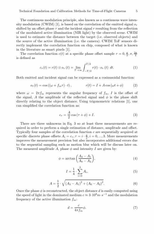
Most of the ToF manufacturers built-in the following principle in their camerassuch as pmdtechnologies1, Mesa Imaging2 or Soft Kinetic3 (cf. Fig. 1). Thesecameras are able to retrieve 2.5D image at a frame rate of 30FPS; pmdtechnolo-gies is currently working on faster device (such as the Camboard Nano) whichoperates at 90FPS. Note that common ToF cameras usually use high modulationfrequency range that make them suitable for near or middle range applications.

Fig. 1. Different ToF phase based camera models available in the market. A PMDCamCube 2.0 (left), a swissranger SR 400 (middle) and a DepthSense DS325 (right).

1 http://www.pmdtec.com/2 http://www.mesa-imaging.ch/3 http://www.softkinetic.com/

Technical Foundation and Calibration Methods for Time-of-Flight Cameras 5

The continuous modulation principle, also known as a continuous wave inten-sity modulation (CWIM) [1], is based on the correlation of the emitted signal oτshifted by an offset phase τ and the incident signal r resulting from the reflectionof the modulated active illumination (NIR light) by the observed scene. CWIMis used to estimate the distance between the target (i.e. observed objects) andthe source of the active illumination (i.e. the camera). CWIM ToF sensors di-rectly implement the correlation function on chip, composed of what is knownin the literature as smart pixels [1].

The correlation function c(t) at a specific phase offset sample τ = 0, π2 , π,

3π2

is defined as

cτ (t) = r(t) ⊗ oτ (t) = limT→∞

∫ T/2

−T/2

r(t) · oτ (t) dt. (1)

Both emitted and incident signal can be expressed as a cosinusoidal function:

oτ (t) = cos ((ω + fmτ) · t) , r(t) = I +A cos (ωt+ φ) (2)

where ω = 2πfm represents the angular frequency of fm, I is the offset ofthe signal, A the amplitude of the reflected signal and φ is the phase shiftdirectly relating to the object distance. Using trigonometric relations [1], onecan simplified the correlation function as:

cτ =A

2cos (τ + φ) + I. (3)

There are three unknowns in Eq. 3 so at least three measurements are re-quired in order to perform a single estimation of distance, amplitude and offset.Typically four samples of the correlation function c are sequentially acquired atspecific discrete phase offsets Ai = cτ , τ = i · π

2 , i = 0, ..., 3. More measurementsimproves the measurement precision but also incorporates additional errors dueto the sequential sampling such as motion blur which will be discuss later on.The measured amplitude A, phase φ and intensity I are given by:

φ = arctan

(A3 −A1

A0 −A2

), (4)

I =1

4·

3∑i=0

Ai, (5)

A =1

2·√(A3 −A1)

2+ (A0 −A2)

2. (6)

Once the phase φ is reconstructed, the object distance d is easily computed usingthe speed of light in the dominated medium c ≈ 3·108m·s−1 and the modulationfrequency of the active illumination fm:

d =c

4πfmφ. (7)

6 D. Lefloch et al.

Since the described principle is mainly based on phase shift calculation, onlya range of distances within one unambiguous range [0, 2π] can be retrieved.This range depends on the modulation frequency fm used during the acquisitiongiving a maximum distance of dmax = c

2fmthat can be computed. Note that the

factor 2 here is due to the fact that the active illumination needs to travel backand forth between the observed object and the camera. It is understood that inthis simple depth retrieval calculation from the phase shift, φ, simplifications aremade which leads to possible measurement errors, e.g the assumption that theactive illumination module and the ToF sensors are placed in the same positionin space; which is physically impossible.

1.2 Pulse Based Approach

Conversely, pulse modulation is an alternative time-of-flight principle which gen-erates pulse of light of known dimension coupled with a fast shutter observation.The 3DV System camera is using this class of technology also known as shut-tered light-pulse (SLP) sensor in order to retrieve depth information. The basicconcept lies on the fact that the camera projects a NIR pulse of light with knownduration (i.e. known dimension) and discretized the front of the reflected illumi-nation. This discretization is realized before the returning of the entire light pulseusing a fast camera shutter. The portion of the reflected pulse signal actuallydescribes the shape of the observed object. Conversely to the unambiguous rangeseen in continuous modulation approach, the depth of interest is directly linkedto the duration of the light pulse and the duration of the shutter (tpulse+δs). Thisphenomenon is known as light wall. The intensity signal capture by the sensorduring the shutter time is strongly correlated with the depth of the observedobject. Since nearer object will appear brighter. This statement is not fully ex-act, since the intensity signal also depends of the observed object reflectivityproperty. As Davis stated [2], double pulse shuttering hardware provide a betterdepth measurement precision than the ones based on a single shutter.

Note that shuttered light-pulse cameras are also subject to similar errors in-troduced in Sec. 1. But due to the fact that this type of cameras are not easilyavailable and that less calibration methods were specially designed for it, we willconcentrate in the following sections on continuation modulation approach.

2 Error Sources

In this section, a full understanding of ToF camera error sources is developed(errors identification and explanation). Calibration approaches that tackle theintrinsic errors of the sensor to correct incorrect depth measurements are pre-sented in Sec. 3. Errors based of extrinsic influences, such as multi-path reflectionor motion can be corrected with methods presented in Sec. 4.

Technical Foundation and Calibration Methods for Time-of-Flight Cameras 7

Beside integration time, that directly influences the signal-to-noise ratio (SNR)of the measurement and consequently the variance of the measured distance, theuser can influenced the quality of the measurements made by setting the fm valueto fit the application. As stated by Lange [1], as fm increases the depth resolutionincreases but the non ambiguity range decreases.

2.1 Systematic Distance Error

Systematic errors occur when the formulas used for the reconstruction do notmodel all aspects of the actual physical imager. In CWIM cameras a prominentsuch error is caused by differences between the actual modulation and correlationfunctions and the idealized versions used for calculations. In case of a sinusodialmodulation Sec. 1.1 , higher order harmonics in the modulating light source(Fig. 2.1) induce deviations from a perfect sine function.Use of the correlationof the physical light source with the formulas 1.1 lead to a periodic ”wiggling”error which causes the calculated depth to oscillate around the actual depth.The actual form of this oscillation depends on the strength and frequencies ofthe higher order harmonics. [1,3].

Fig. 2. Left:Measured modulation of the PMD light source: Right: Mean depth devia-tion as a function of the real distance. Images from [4].

There are two approaches for solving this problem. The first approach is tosample the correlation more phase shifts and extend the formulas to incorporatehigher order harmonics[5]. With current 2-tap sensor this approach induces moreerrors when observing dynamic scenes. The second approach which we will fur-ther discuss in 3.2 is to keep the formulas as they are and estimate the residualerror between true and calculated depth [6,7] . The residual can then be usedin a calibration step to eliminate the error. Finally, [8] employ a phase modu-lation of the amplitude signal to attenuate the higher harmonics in the emittedamplitude.

8 D. Lefloch et al.

2.2 Intensity-Related Distance Error

In addition to the wiggling systematic error, the measured distance is greatlyaltered by an error dependent of the total amount of incident light recieved bythe sensor. Measured distance of lower reflectivity objects appear closer to thecamera (up to 3cm drift for the darkest objects). Fig. 3 highlights this erroreffect using a simple black-and-white checkerboard pattern. The described erroris usually known as Intensity-related distance error and its cause is not fullyunderstood yet [9].

Nevertheless, recent investigation [10] shows that ToF sensor has a non-linearresponse during the conversion of photons to electrons. Lindner et al. [9] claimsthat the origin of the intensity-related error is assumed to be caused by non-linearities of the semi conductor hardware.

A different point of view would be to consider the effect of multiple returnscaused by inter-reflections in the sensor itself (scattering between the chip andthe lens). Since the signal strength of low reflectivity objects is considerablyweak, they will be more affected by this behavior than for high signal strengthgiven by brighter objects. For more information about multi-path problems onToF cameras, referred to Sec. 2.5.

Fig. 3. Impact of the intensity-related distance error on the depth measurement: Leftimage shows the intensity image given by a ToF camera. Right image shows the surfacerendering obtained by the depth map colored by its corresponding intensity map. Notethat those images were acquired using a PMD CamCube 2.0, PMDTechnologies GmbH

2.3 Depth Inhomogeneity

An important type of errors in ToF imaging, the so-called flying pixels, occursalong depth inhomogeneities. To illustrate these errors, we consider a depthboundary with one foreground and one background object. In the case that thesolid angle extent of a sensor pixel falls on the boundary of the foreground andthe background, the recorded signal is a mixture of the light returns from bothareas. Due to the non-linear dependency of the depth on the raw channels and

Technical Foundation and Calibration Methods for Time-of-Flight Cameras 9

the phase ambiguity, the resulting depth is not restricted to the range betweenforeground and background depth, but can attain any value of the camera’sdepth range. We will see in Section 4.1, that is important to distinguish betweenflying pixels in the range of the foreground and background depth and outliers.The fact that today’ ToF sensors provide only a low resolution promotes theoccurrence of flying pixels of both kinds.

We remark that the problem of depth inhomogeneities is related to the mul-tiple return problem, since also here light from different paths is mixed in onesensor cell. In the case of flying pixels, however, local information from neigh-boring pixels can be used to approximately reconstruct the original depth. Werefer to Section 4.1 for details.

2.4 Motion Artifacts

As stated in 1.1, CWIM ToF imagers need to sample the correlation betweenincident and reference signal at least using 3 different phase shifts. Ideally theseraw images would be acquired simultaneously. Current two tap sensors onlyallow for two of these measurements to be made simultaneously such that atleast one more measurement is needed. Usually, further raw images are acquiredto counteract noise and compensate for different electronic charateristics of theindividual taps. Since these (pairs) of additional exposures have to be madesequentially, dynamic scenes lead to erroneous distance values at depth andreflectivity boundaries.

Methods for compensating motion artifacts will be discussed in Section 4.2.

2.5 Multiple Returns

The standard AMCW model for range imaging is based on the assumption thatthe light return to each pixel of the sensor is from a single position in the scene.This assumption, unfortunately, is violated in most scenes of practical interest,thus multiple returns of light do arrive at a pixel and generally lead to erroneousreconstruction of range at that pixel. Multiple return sources can be categoriseddue to two primary problems. Firstly, the imaging pixel views a finite solid angleof the scene and range inhomogeneities of the scene in the viewed solid anglelead to multiple returns of light—the so-calledmixed pixed effect which results inflying pixels (see Section 2.3 above). Secondly, the light can travel multiple pathsto intersect the viewed part of the scene and the imaging pixel—the multipathinteference problem. Godbaz [11] provides a thorough treatment of the multiplereturn problem, including a review covering full field ToF and other rangingsystems with relevant issues, such as point scanners.

In a ToF system light returning to the sensor is characterised by amplitude Aand phase shift φ. The demodulated light return is modelled usefully as thecomplex phasor

η = Aejφ, (8)

10 D. Lefloch et al.

φ1

η1

I

R

ξ

φ2η2

Fig. 4. Phasor diagram of the demodulated output in complex form. The primaryreturn, η1, is perturbed by a secondary return, η2, resulting in the measured phasor, ξ.

where j =√−1 is the imaginary unit. When light returns to a pixel via N mul-

tiple paths then the individual return complex phasors add yielding a totalmeasurement ξ given by

ξ =

N∑n=1

ηn =

N∑n=1

Anejφn . (9)

One of the phasors is due to the primary return of light, namely that of theideal path intended in the design of the imaging system. Note that the primaryreturn is often the brightest return, though it need not be. Let us take η1 as theprimary return and every other return (η2, η3, etc.) as secondary returns arisingfrom unwanted light paths. A diagram of the two return case is shown in Fig. 4.Note that when the phase of the second return φ2 changes, the measured phasorξ changes both in amplitude and phase.

It is useful to categorise multiple returns due to multipath interference as tothose that are caused by scattering within the scene and those resulting fromscattering within the camera. Scene based multi-path interference arises due tolight reflecting or scattering off multiple points in the scene to arrive at the samepixel of the sensor, and is frequently the most obvious effect to see in a ToF rangeimage. The following example illustrates a common situation. Consider a scenewhere there is a large region of shiny floor exhibiting specular reflection. Whenlight diffusely reflects off some other surface, such as a wall or furniture, a portionof that light is diffusely reflected so that it travels down towards the floor. When

Technical Foundation and Calibration Methods for Time-of-Flight Cameras 11

the ToF camera is viewing the floor and wall a hole is reconstructed in the floor,where the position of the hole aligns with the light path from camera to wall,wall to floor, and then back to the camera. The distance into the hole is dueto the phase of the total measured phasor and is determined by the relativeamplitude and phase of the component returns, as per Eq. 9. Another examplethat exhibits strong multipath interference is the sharp inside corner junctionbetween two walls [12]. The light bouncing from one wall to the other causes thecamera to measure an erroneous curved corner.

Multipath interference can also occur intra-camera due to the light refractionand reflection of an imaging lens and aperture [13,14,15]. The aperture effectis due to diffraction which leads to localised blurring in the image formationprocess. Fine detail beyond the limits in angular resolution is greatly reduced,causing sharp edges to blur. Aberrations in the lens increase the loss in resolu-tion. Reflections at the optical boundaries of the glass produce what is commonlyreferred to as lens flare [16], which causes non-local spreading of light across thescene. In ToF imaging the lens-flare effect is most prominent when a bright fore-ground scatterer is present. The foreground object does not need to be directlyvisible to the camera, as long as the light from the source is able to reach thatobject and reflect, at least in part, back to the lens [17]. Such light scatteringleads to distorted reconstructed ranges throughout the scene with the greatesterrors occurring for darker objects.

2.6 Other Error Sources

ToF camera sensors suffer from the same errors as standard camera sensors. Themost important error source in the sensor is a result of the photon countingprocess in the sensor. Since photons are detected only by a certain probability,Poisson noise is introduced. We refer to Seitz [18] and the thesis by Schmidt [10,Sect. 3.1] for detailed studies on the Poisson noise. An experimental evaluationof noise characteristics of different ToF cameras has been performed in by Erz& Jahne [19]. Besides from that other kinds of noise, e.g. dark (fixed-pattern)noise and read-out noise, occur.

In ToF cameras, however, noise has a strong influence on the estimated scenedepth, due to the following two issues

– The recorded light intensity in the raw channels is stemming from both activeand background illumination. Isolating the active part of the signal reducesthe SNR. Such a reduction could be compensated by increasing the integra-tion time, which on the other hand increases the risk of an over-saturation ofthe sensor cells, leading to false depth estimation. As a consequence, a trade-off in the integration time has to be made, often leading to a low SNR in theraw data, which occurs especially in areas with extremely low reflectivity orobjects far away from the sensor.

– Since the estimated scene depth depends non-linearly on the raw channels(cf. Eqs. 4 and 7), the noise is amplified in this process. This amplification istypically modeled ([1,20]) by assuming Gaussian noise in the raw data and

12 D. Lefloch et al.

performing a sensitivity analysis. By this simplified approach, it turns outthat the noise variance in the final depth estimates depend quadratically onthe amplitude of the active illumination signal. In particular, the variancecan change drastically within the different regions of the scene depending onthe reflectivity and the distance of the objects.

Due to these short-comings current ToF cameras have a resolution smaller thanhalf VGA, which is rather small in comparison to standard RGB or grayscalecameras.

We remark that the noise parameters of ToF cameras are part of the EMVAstandard 1228[21], thus they are assumed to be provided in the data sheet, ifthe ToF camera conforms to the standard.

We finally consider a scenario, where several ToF cameras are used to retrievedepth maps of a scene from different viewpoints. As a consequence of the modu-lation of the active illumination, the emitted light of each camera can affect therecordings of the other cameras, leading to false depth estimates. Some cameramanufacturers account for this issue by allowing to change the modulation inthe camera settings. In case that the modulation frequency of one sensor doesnot match the frequency of the light from a different light source, the effect ofinterference can be reduced as long as the integration time for the raw channelsis far larger than 1

fm.

3 Calibration Approaches

In this section, the approaches to handle individual error sources are explained indetail. First a foundation on standard camera calibration techniques is presentedto be followed by ToF depth calibration and depth enhancement.

3.1 Standard Camera Calibration

Optical camera calibration is one of the basic requirements before precise mea-surements can be performed. The optical lens configuration and the cameraassembly determine the optical path of the light rays reaching each pixel. Onehas to distinguish between the camera-specific parameters that determine theoptical rays in camera-centered coordinates, termed intrinsic calibration, andthe extrinsic calibration which determines the 3D position and 3D orientation(the pose) of the camera coordinate system in 3D world coordinates.

Typically, the intrinsic parameters are defined by the linear calibration matrix,K, which holds the camera focal length f , the pixel size sx, sy, and the opticalimage center cx, cy of the imaging chip. In addition, non-linear image distortioneffects from the lens-aperture camera construction have to be included, which canbe severe in cheap cameras and for wide-angle lenses. A polynomial radial andtangential distortion function is typically applied to approximate the distortioneffects. Radial-symmetric and tangential coefficients for polynomials up to 3rdorder are included in the intrinsic calibration.

Technical Foundation and Calibration Methods for Time-of-Flight Cameras 13

Unfortunately, it is very difficult to determine the intrinsic parameters byinspecting the optical system directly. Instead, intrinsic and extrinsic parametershave to be estimated jointly. A known 3D reference, the calibration object, isneeded for this task, since it allows to relate the light rays emitted from known3D object points to the 2D pixel in the camera image plane. A non-planar 3Dcalibration object with very high geometric precision is preferred in high-qualityphotogrammetric calibration, but these 3D calibration objects are difficult tomanufacture and handle, because they ideally should cover the complete 3Dmeasurement range of the camera system. In addition, when calibrating notonly optical cameras but also depth cameras, the design of such 3D pattern isoften not possible due to the different imaging modalities of depth and color.

Therefore, a planar 2D calibration pattern is preferred which allows a mucheasier capture of the calibration data. A popular approach based on a 2D pla-nar calibration pattern was proposed by Zhang[22]. The 2D calibration objectdetermines the world coordinate system, with the x-y coordinates spanning the2D calibration plane, and the z coordinate spanning the plane normal direction,defining the distance of the camera center from the plane. For 3D point identi-fication, a black and white checkerboard pattern is utilized to define a regularspacing of known 3D coordinates. In this case, a single calibration image is notsufficient, but one has to take a series of different calibration images while mov-ing and tilting the calibration plane to cover the 3D measurement range of thesystem. For each image, a different extrinsic camera pose has to be estimated,but all intrinsic parameters remain fixed and are estimated jointly from the im-age series. This is advantageous, since some of the calibration parameters arehighly correlated and need disambiguation. For example, it is difficult to distin-guish between the extrinsic camera distance, z, and the intrinsic focal length,f, because f is similar to a simple magnification and inversely proportional toz. However, if sufficiently many different camera distances are recorded in thecalibration sequence, one can distinguish them from the constant focal length.

Another source of error during calibration is the optical opening angle of thecamera, the field of view fov. Calibration of a camera with narrow fov leadsto high correlation between extrinsic position and orientation, because movingthe camera in the x-y plane and simultaneous rotating it to keep the camerafocused on the same part of the calibration pattern is distinguishable only bythe perspective distortions in the image plane due to out-of-plane rotation of thecalibration object[23,7]. Hence it is advisable to employ wide-angle cameras, ifpossible, for stable extrinsic pose estimation. Brought to the extreme, one wouldlike to use omnidirectional or fisheye cameras with extremely large fov for bestpossible extrinsic pose estimation. In this case, however, it is also advisable toincrease the available image resolution as much as possible, since for large fovoptics the angular resolution per pixel decreases. See [24] for a detailed analysis.

The focus of this contribution is to calibrate a tof depth camera from imagedata. Given the above discussion, it is clear that this will be a difficult prob-lem. The cameras typically have a limited fov by construction, since its infraredlighting has to illuminate the observable object region with sufficient intensity.

14 D. Lefloch et al.

Thus, wide fov illumination is not really an option, unless in very restrictedsituations. In addition, the image resolution is typically much lower than withmodern optical cameras, and this will not change soon due to the large pixel sizeof the correlating elements. Finally, no clear optical image is captured but onlythe reflectance image can be utilized for calibration. Early results show that thequality of the calibration using the approaches as described above is poor[6,25].

However, there is also an advantage of using depth cameras, since the cameradistance z can be estimated with high accuracy from the depth data, eliminatingthe f/z ambiguity. The calibration plane can be aligned with all depth measure-ments from the camera by plane fitting. Hence, all measurements are utilizedsimultaneously in a model-based approach that compares the estimated planefit with the real calibration plane. More general, a virtual model of the calibra-tion plane is built, including not only geometry but also surface color, and issynthesized for comparison with the observed data. This model-driven analysis-by-synthesis approach exploits all camera data simultaneously, and allows furtheron to combine the ToF camera with additional color cameras, which are rigidlycoupled in a camera rig. The coupling of color cameras with depth cameras isthe key to high-quality calibration, since it combines the advantages of colorand depth data. High-resolution color cameras with large fov allow a stable andaccurate pose estimation of the rig, while the depth data disambiguates z fromf . The synthesis part is easily ported to GPU-Hardware, allowing for fast cali-bration even with many calibration images4. For details about this approach werefer to [26,7]. The approach allows further to include non-linear depth effects,like the wiggling error, and reflectance-dependent depth bias estimates into thecalibration[27]. Depth calibration will be discussed next.

3.2 Depth Calibration

As described in 2, there are several reasons for a deviation of actual depth anddepth measured by the ToF camera. To record accurate data, a thorough depthcalibration has to be done. It should be noted here, that since the ToF camerameasures the time of flight along the light path of course, error calibration shouldbe done with respect to the radial distance as well, not in Cartesian coordinates.

One of the first contributions to this topic is [6] by Lindner and Kolb. Theycombined a pixelwise linear calibration with a global B-splines fit. In [7] Schilleret. al. used a polynomial to model the distance deviation.

Since a large share of the deviation is due to the non-sinusoidal illuminationsignal 2.1, an approach modelling this behavior is possible as well, as shown in[10]. But a completely model based behaviour would have to incorporate othererror sources as well, like the intensity related distance error 2.2, which is notyet understood and hence, there is no model to fit to the data.

Lindner and Kolb used two separate B-spline functions to separate the dis-tance and intensity related error in [28], even the integration time is considered

4 Software is available athttp://www.mip.informatik.uni-kiel.de/tiki-index.php?page=Calibration

Technical Foundation and Calibration Methods for Time-of-Flight Cameras 15

by linear interpolation of the control points. The drawback of this method is thelarge amount of data, necessary to determine all the parameters of the compen-sation functions.

Lindner et. al. reduce the amount of necessary data in [27]. They use a mod-ified calibration pattern, a checkerboard with different greylevels and introducea normalization for the intensity data of different depths, reducing the amountof necessary data considerably.

Temperature Drift

9400 9600 9800

10000 10200 10400 10600 10800 11000 11200

0 1000 2000 3000 4000 5000 6000 7000 8000

inte

nsity

[1]

time [s]

2010

2015

2020

2025

2030

2035

2040

2045

0 1000 2000 3000 4000 5000 6000 7000 8000

ampl

itude

[1]

time [s]

3.3

3.31

3.32

3.33

3.34

3.35

3.36

3.37

0 1000 2000 3000 4000 5000 6000 7000 8000

dept

h [m

]

time [s]

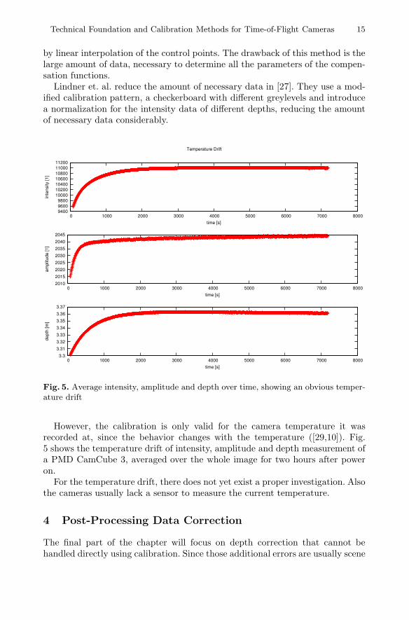
Fig. 5. Average intensity, amplitude and depth over time, showing an obvious temper-ature drift

However, the calibration is only valid for the camera temperature it wasrecorded at, since the behavior changes with the temperature ([29,10]). Fig.5 shows the temperature drift of intensity, amplitude and depth measurement ofa PMD CamCube 3, averaged over the whole image for two hours after poweron.

For the temperature drift, there does not yet exist a proper investigation. Alsothe cameras usually lack a sensor to measure the current temperature.

4 Post-Processing Data Correction

The final part of the chapter will focus on depth correction that cannot behandled directly using calibration. Since those additional errors are usually scene

16 D. Lefloch et al.

dependent (as dynamic environment), a last processing needs to be applied afterthe depth correction via calibration in order to increase the reliability of ToFrange measurements.

This section is divided into three subsections and will present state-of-the-arttechniques to correct the remaining errors.

4.1 Depth Inhomogeneity and Denoising

For the task of denoising Time-of-Flight data, we refer to Chapter 2, Section 2,where state-of-the-art denoising methods and denoising strategies are discussedin detail. In the following, we focus on the problem of flying pixels. We distinguishbetween methods which directly work on the 2D output of the ToF cameras andmethods which are applied after interpreting the data as 3D scenes, e.g. as pointclouds.

On methods applied to the 2D data we remark that median filtering is a simpleand efficient means to for a rough correction of flying pixels, which are outsidethe objects’ depth range. We refer to [30] for a more involved filtering pipeline.In addition, we remark that denoising methods to a certain extend are capableof dealing with such kind flying pixels. This is due to the fact that regions ofdepth inhomogeneities are typically one dimensional structures and flying pixelsappear only in a narrow band along these regions. As a consequence, out-of-rangeflying pixels can be regarded as outliers in the depth measurement. Denoisingmethod in general are robust against such outliers, and produces reconstructionswith a certain spatial regularity. The correction of in-range flying pixels is muchmore involved. The standard approach is to identify such pixels, e.g. by confi-dence measures [31] and to discard them. The depth value of the discarded pixelthen has to be reconstructed using information from the surrounding pixels. Inparticular, the pixel has to be assigned to one of the adjacent objects. Super-resolution approaches [32,33] allow to assign parts the pixel area to each of theobjects.

Also when considering 3D data (point clouds), geometrical information canbe used to correct for flying pixels, for example by clustering the 3D data inorder to determining the underlying object surface (e.g. [34,35]).

Finally, flying pixels can be dealt with when fusing point clouds [36,37] fromdifferent sources with sub-pixel accuracy. Here, it is substantial to reliably iden-tify flying pixels, so that they can be removed before the actual fusion process.Missing depth data then is replaced by input from other sources. In order toidentify flying pixels, confidence measures [31] for ToF data can be taken intoaccount.

4.2 Motion Compensation

As stated in 2.4, motion artifacts occur in dynamic scenes at depth and reflectiv-ity boundaries due to the sequential sampling of the correlation function. Thereare three (or arguably two) different approaches to reduce such artifacts. Oneway is by decreasing the number of frames obtained sequentially and needed to

Technical Foundation and Calibration Methods for Time-of-Flight Cameras 17

produce a valid depth reconstruction. As current two-tap sensors have differentelectronic characteristics for each tap, the raw values belonging to different tapscannot be combined without further calibration. In 4.2.1 a method proposed bySchmidt et al. [10] will be presented where each of these taps are dynamically cal-ibrated, such that a valid measurement can be obtained with the bare minimumof 2 consecutive frames. Another approach commonly employed is composed ofa detection step, where erroneous regions due to motion are found, followed bya correction step. The methods presented in 4.2.2 differ how these two steps areundertaken and in how much knowledge of the working principles is put in to thesystem. The final approach proposed by Lindner et al [38] is to directly estimatescene motion between sub-frames using optical flow. This approach can be seenas an extension of the detect and repair approach, but as the detection is notonly binary and the correction not only local it will be presented separately in4.2.3.

4.2.1 Framerate EnhancementCurrent correlating pixels used in ToF cameras are capable of acquiring Q =2 phase images simultaneously, shifted by 180 degrees. N of these simultane-ous measurements are made sequentially to obtain a sufficient sampling of thecorrelation function.

Table 1. Illustration of raw frame yphaseindex,tapindex for Q = 2 taps and N = 4acquisitions

time t0 t1 t2 t3tap 0 y0,0 y1,0 y2,0 y3,0tap 1 y3,1 y2,1 y1,1 y0,1

As shown by Erz et al [19,39] these taps have different amplification char-acteristics, such that the raw values obtained from the taps cannot directly beused. Instead N has to be chosen as 4. and the Ai used in Eq. 3 calculated as

Ai =

Q∑k=0

yi,k (10)

The relationship between the different taps is given implicitly per pixel by

yi,0 = ri,k(yi,k) (11)

Schmidt [10] models these ri,k as a linear polynomial and proposes a dynamiccalibration scheme to estimate them. For different intensity and depth staticsequences are obtained and a linear model fitted between yi,0 and yi,k. The fullmodel with further extensions such as interleaved calibration can be found in[10]. Note that this only reduces, but does not eliminate motion artifacts.

18 D. Lefloch et al.

4.2.2 Detect and Repair MethodsDetect and repair approaches can be further categorized in methods that operatedirectly on the depth image [40,41] and the methods that harness the relationbetween the raw data channels [10,42,43].

Filter based methodsGokturk et al. [40] applied morphological filters on a foreground/background seg-mented depth image to obtain motion artifact regions. These pixels are replacedby synthetic values using a spatial filtering process. Lottner et al. [41] proposedto employ data of an additional high resolution 2D sensor being monocularlycombined with the 3D sensor, effectively suggesting a joint filtering approachwhich uses the edges of the 2d sensor to guide the filter.

Methods operating on raw dataDetection Schmidt [10] calculates the temporal derivatives of the individualraw frames. Motion artifacts occur if the first raw frame derivative is near 0 (nochange) whereas one of the other raw frames has a large derivative. This meansthat movement occured between sub-frames. Lee et al. [43] operates on a similarprinciple. But evaluates the sums of two sub-frames.

Correction Finally once regions with artifacts are detected, they need to berepaired in some where. Here Schmidt uses the last pixel values with valid rawimages whereas Lee uses the spatially nearest pixel with valid data.

Correction Finally once regions with artifacts are detected, they need to berepaired in some way. Here Schmidt uses the last pixel values with valid rawimages whereas Lee uses the spatially nearest pixel with valid data.

4.2.3 Flow Based Motion CompensationSo far, the detection step gave a binary output whether or whether not mo-tion was present in a pixel. Subsequently some heuristic was applied to inpaintthe regions with detected motion. Lindner et al. [38] took a somewhat differentapproach by loosening the requirement that the 4 measurements used for recon-struction need to originate from the same pixel. Instead, the ”detection” is doneover the whole scene by estimating the optical flow between sub-frames. Theapplication of optical flow to the raw data and the subsequent demodulation atdifferent pixel positions require the following two points to be considered:

– Brightness constancy (corresponding surface points in subsequent sub-framesshould have the same brightness to be able to match). This is not the case forthe raw channels due to the internal phase shift between modulated and ref-erence signal. Fortunately, in multi-tap sensors, the intensity (total amountof modulated light) can be obtained by adding up the measurements in dif-ferent taps. Thus, the brightness constancy is given between the intensity ofsub-frames:

Ii =

Q∑j=0

ui,j (12)

Technical Foundation and Calibration Methods for Time-of-Flight Cameras 19

– Pixel Homogeneity. The application of the demodulation at different pixellocations requires a homogeneous sensor behavior over all locations. Other-wise artifacts will be observed which usually cancel out by using the samepixel for all four measurements. Again, this is not the case for the raw chan-nels due to pixel gain differences and a radial light attenuation toward theimage border. To circumvent this, Lindner et al. [38] proposed a raw valuecalibration based on work by Sturmer et al. [44].

Once the flow is known, it can be used to correct the raw image before applyingthe standard reconstruction formulas. The strength and weakness of this methodis strongly coupled with the flow method used. It is important to obtain thecorrect flow especially at occlusion boundaries, such that discontinuity preservingflow methods should be preserved. Lindner et al. [38] reported a rate of 10 framesper second using the GPU implemented version TV-L1 flow proposed by Zach etal. [45] on a 2009 machine. Lefloch et al. [46] has recently proposed an alternativesolution, based on the previous work of Lindner et al., in order to improve theperformance of the motion compensation by reducing the number of computedsubsequent optical flows.

4.3 Multiple Return Correction

The determination of the multiple returns of multipath or mixed pixels essen-tially is the separation of complex phasors into two or more components. Giventhe complex measurement arising from the demodulation, Eq. 9, correction isthe separation of the total phasor into its constituent returns. The problem ofmultiple return correction of a single range image is underdetermined as only onecomplex measurement is made but the signal at each pixel is the linear combi-nation (in the complex plane) of more than one return. To separate out multiplereturns more information is needed, either in the form of a priori assumptionsor multiple measurements.

Iterative offline processing of range images has been used to demonstratesucessful separation of multiple returns [47], however the algorithm is not suitablefor realtime operation. Here we summarise the work of Godbaz [11], who pro-vides a mathematical development that leads to a fast online algorithm. Godbazemploys multiple measurements with the assumption that two returns dominatethe measurement process, thus requiring at least two measurements for returnseparation. Note that a fully closed form solution is possible for the overdeter-mined case of three or more measurements and two returns [11,48].

We begin by writing Eq. 9 for two returns with the implicit assumption thatthe measurement is taken at camera modulation frequency f1, namely

ξ1 = η1 + η2. (13)

Now, consider measurement at a second frequency fr = rf1, where r is therelative frequency between fr and f1. A measurement at relative frequency r is

ξr =ηr1

|η1|r−1+

ηr2|η2|r−1

. (14)

20 D. Lefloch et al.

Qualitatively, the action of making a new measurement at relative frequency rrotates each component return so that its phase is increased to r times its originalwhile leaving the amplitude unchanged.5 This phase rotation is the informationthat is exploited to separate the returns. It can be shown that the measurementmade at relative frequency r factorises as

ξr =ηr1

|η1|r−1Λr(b, θ), (15)

where Λr(b, θ) = 1 + bejrθ (16)

with b =|η2||η1| , (17)

and θ = φ2 − φ1. (18)

Here b and θ are the relative amplitude and phase and describe the perturba-tion of the primary return by the secondary return. From these we obtain thecharacteristic measurement, χ, defined by

χ =ξr|ξ1|r−1

ξr1(19)

=Λr(b, θ)|Λ1(b, θ)|r−1

Λ1(b, θ)r. (20)

The computation of χ normalises for the primary return, yielding a number thatis explicitly dependent on b and θ.

A look-up table of the inverse of Eq. 20 can be constructed using parametriccurve fitting. Given indices |χ| and argχ into the table, b and θ are read fromthe look-up table, Λ1(b, θ) is computed, and the estimate of the primary returnis simply

η1 =ξ1

Λ1(b, θ). (21)

The relative frequency r = 2 is used in the implementation described by God-baz [11], with the development and merit of other frequency ratios also consid-ered. It is important to note that the characteristic measurement χ is multi-valued thus multiple solutions arise in calculating its inverse. For the case r = 2there are two solutions, but there is a symmetry in Λr(b, θ) that leads to a degen-eracy. The two solutions are equivalent up to the fact that the second solutionphysically corresponds to solving for η2 in Eq. 21.

The multiple return correction is demonstrated using the Mesa ImagingSR4000 camera with a frequency combination of 15:30 MHz. An amplitude andphase pair is shown in Fig. 6 of a scene of a hallway with a shiny floor and a

5 The assumption of invariance of the component amplitude with respect to a change inmodulation frequency is an ideal one. In practice factors arising due to the light andsensor modulation mean that a calibration of amplitude with respect to frequencyis required.

Technical Foundation and Calibration Methods for Time-of-Flight Cameras 21

10 m

0 m

Fig. 6. The amplitude (left) and phase (right) of a range image pair. The reflection ofa bright white circular object manifests as multipath returns from the floor.

10 m

0 m

Fig. 7. The estimated primary (left) and secondary (right) returns

target object of a black board with a large round white circle. The board is 4.5 mfrom the camera. The effect of the reflection of the white circle is visible on thefloor near the bottom of both the amplitude and phase images. The estimates ofthe primary and secondary returns are shown in Fig. 7. The appearance of thephase shift induced by the reflection of the white circle is greatly reduced in theprimary return estimate. Godbaz [11] analysed the noise behaviour of multiplereturn correction and found an increase in noise, as is seen when comparing theprimary return estimate with the distance measurement.

5 Conclusion

In this paper, we present state-of-the art techniques that improved significantlyraw data given by ToF sensors. We have seen that ToF cameras are subject toa variety of errors caused by different sources. Some errors can be handled bysimple calibration procedure, nevertheless other sources of errors are directlyrelated to the observed scene configuration which thus require post processingtechniques. Nevertheless, there are still some open issues that need to be further

22 D. Lefloch et al.

investigated. One concerns the intensity-related distance error which is, as statedpreviously, not fully yet understood. The second open issue lies on multi-pathproblem where separation of global and local illumination is required to providea reliable correction. Finally, there are still some difficulties for researchers toevaluate their work since groundtruth generation is still an open issue.

References

1. Lange, R.: 3D Time-of-Flight Distance Measurement with Custom Solid-State Im-age Sensor in CMOS/CCD-Technology. PhD thesis (2000)

2. Davis, J., Gonzalez-Banos, H.: Enhanced shape recovery with shuttered pulses oflight. In: Pulses of Light? IEEE Workshop on Projector-Camera Systems (2003)

3. Rapp, H.: Experimental and theoretical investigation of correlating tof-camera sys-tems. Master’s thesis (2007)

4. Schmidt, M., Jahne, B.: A physical model of time-of-flight 3D imaging systems,including suppression of ambient light. In: Kolb, A., Koch, R. (eds.) Dyn3D 2009.LNCS, vol. 5742, pp. 1–15. Springer, Heidelberg (2009)

5. Dorrington, A.A., Cree, M.J., Carnegie, D.A., Payne, A.D., Conroy, R.M., Godbaz,J.P., Jongenelen, A.P.: Video-rate or high-precision: A flexible range imaging cam-era. In: Electronic Imaging 2008, International Society for Optics and Photonics,pp. 681307–681307 (2008)

6. Lindner, M., Kolb, A.: Lateral and depth calibration of pmd-distance sen-sors. In: Bebis, G., Boyle, R., Parvin, B., Koracin, D., Remagnino, P., Ne-fian, A., Meenakshisundaram, G., Pascucci, V., Zara, J., Molineros, J., Theisel,H., Malzbender, T. (eds.) ISVC 2006. LNCS, vol. 4292, pp. 524–533. Springer,Heidelberg (2006)

7. Schiller, I., Beder, C., Koch, R.: Calibration of a pmd camera using a planar cali-bration object together with a multi-camera setup. In: The International Archivesof the Photogrammetry, Remote Sensing and Spatial Information Sciences, PartB3a, Beijing, China, vol. XXXVII, pp. 297–302 XXI. ISPRS Congress (2008)

8. Payne, A.D., Dorrington, A.A., Cree, M.J., Carnegie, D.A.: Improved measurementlinearity and precision for amcw time-of-flight range imaging cameras. AppliedOptics 49(23), 4392–4403 (2010)

9. Lindner, M.: Calibration and Real-Time Processing of Time-of-Flight Range Data.PhD thesis, CG, Fachbereich Elektrotechnik und Informatik, Univ. Siegen (2010)

10. Schmidt, M.: Analysis, Modeling and Dynamic Optimization of 3D Time-of-FlightImaging Systems. PhD thesis, IWR, Fakultat fur Physik und Astronomie, Univ.Heidelberg (2011)

11. Godbaz, J.P.: Ameliorating systematic errors in full-field AMCW lidar. PhD thesis,School of Engineering, University of Waikato, Hamilton, New Zealand (2012)

12. A., G.S., Aanaes, H., Larsen, R.: Environmental effects on measurement uncer-tainties of time-of-flight cameras. In: Proceedings of International Symposium onSignals, Circuits and Systems 2007, ISSCS 2007 (2007)

13. Shack, R.V.: Characteristics of an image-forming system. Journal of Research ofthe National Bureau of Standards 56(5), 245–260 (1956)

14. Barakat, R.: Application of the sampling theorem to optical diffaction theory. Jour-nal fo the Optical Society of America 54(7) (1964)

15. Saleh, B.E.A., Teich, M.C.: 10. In: Fundamentals of Photonics, pp. 368–372. JohnWiley and Sons, New York (1991)

Technical Foundation and Calibration Methods for Time-of-Flight Cameras 23

16. Matsuda, S., Nitoh, T.: Flare as applied to photographic lenses. Applied Op-tics 11(8), 1850–1856 (1972)

17. Godbaz, J., Cree, M., Dorrington, A.: Understanding and ameliorating non-linearphase and amplitude responses in amcw lidar. Remote Sensing 4(1) (2012)

18. Seitz, P.: Quantum-noise limited distance resolution of optical range imaging tech-niques. IEEE Transactions on Circuits and Systems I: Regular Papers 55(8),2368–2377 (2008)

19. Erz, M., Jahne, B.: Radiometric and spectrometric calibrations, and distance noisemeasurement of toF cameras. In: Kolb, A., Koch, R. (eds.) Dyn3D 2009. LNCS,vol. 5742, pp. 28–41. Springer, Heidelberg (2009)

20. Frank, M., Plaue, M., Rapp, H., Kothe, U., Jahne, B., Hamprecht, F.A.: Theoreticaland experimental error analysis of continuous-wave time-of-flight range cameras.Optical Engineering 48(1), 13602 (2009)

21. Emva standard 1288 -standard for measurement and presentation of specificationsfor machine vision sensors and cameras, Release 3.0 (2010)

22. Zhang, Z.: A flexible new technique for camera calibration. IEEE Trans. PatternAnal. Mach. Intell. 22(11), 1330–1334 (2000)

23. Beder, C., Bartczak, B., Koch, R.: A comparison of PMD-cameras and stereo-visionfor the task of surface reconstruction using patchlets. In: IEEE/ISPRS BenCOSWorkshop 2007 (2007)

24. Streckel, B., Koch, R.: Lens model selection for visual tracking. In: Kropatsch,W.G., Sablatnig, R., Hanbury, A. (eds.) DAGM 2005. LNCS, vol. 3663, pp. 41–48.Springer, Heidelberg (2005)

25. Kahlmann, T., Remondino, F., Ingensand, H.: Calibration for increased accuracyof the range imaging camera swissrangertm. In: Proc. of IEVM (2006)

26. Beder, C., Koch, R.: Calibration of focal length and 3d pose based on the reflectanceand depth image of a planar object. In: Proceedings of the DAGM Dyn3D Work-shop, Heidelberg, Germany (2007)

27. Marvin, L., Ingo, S., Andreas, K., Reinhard, K.: Time-of-flight sensor calibrationfor accurate range sensing. Comput. Vis. Image Underst. 114(12), 1318–1328 (2010)

28. Lindner, M., Kolb, A.: Calibration of the intensity-related distance error of the pmdtof-camera. In: Proc. SPIE, Intelligent Robots and Computer Vision, vol. 6764, p.67640W (2007)

29. Steiger, O., Felder, J., Weiss, S.: Calibration of time-of-flight range imaging cam-eras. In: 15th IEEE International Conference on Image Processing, ICIP 2008, pp.1968–1971. IEEE (2008)

30. Swadzba, A., Beuter, N., Schmidt, J., Sagerer, G.: Tracking objects in 6d for re-constructing static scenes. In: IEEE Computer Society Conference on ComputerVision and Pattern Recognition Workshops, CVPRW 2008, pp. 1–7. IEEE (2008)

31. Reynolds, M., Dobos, J., Peel, L., Weyrich, T., Brostow, G.J.: Capturing time-of-flight data with confidence. In: 2011 IEEE Conference on Computer Vision andPattern Recognition (CVPR), pp. 945–952. IEEE (2011)

32. Lindner, M., Lambers, M., Kolb, A.: Sub-pixel data fusion and edge-enhanceddistance refinement for 2d / 3d images. International Journal of Intelligent SystemsTechnologies and Applications 5, 344–354 (2008)

33. Pathak, K., Birk, A., Poppinga, J.: Sub-pixel depth accuracy with a time of flightsensor using multimodal gaussian analysis. In: IEEE/RSJ International Conferenceon Intelligent Robots and Systems, IROS 2008, pp. 3519–3524 (2008)

34. Moser, B., Bauer, F., Elbau, P., Heise, B., Schoner, H.: Denoising techniques forraw 3D data of ToF cameras based on clustering and wavelets. In: Proc. SPIE,vol. 6805 (2008)

24 D. Lefloch et al.

35. H., S., Moser, B., Dorrington, A.A., Payne, A., Cree, M.J., Heise, B., Bauer, F.:A clustering based denoising technique for range images of time of flight cameras.In: CIMCA/IAWTIC/ISE 2008, pp. 999–1004 (2008)

36. Schuon, S., Theobalt, C., Davis, J., Thrun, S.: Lidarboost: Depth superresolutionfor tof 3d shape scanning. In: IEEE Conference on Computer Vision and PatternRecognition, CVPR 2009, pp. 343–350. IEEE (2009)

37. Cui, Y., Schuon, S., Chan, D., Thrun, S., Theobalt, C.: 3d shape scanning with atime-of-flight camera. In: 2010 IEEE Conference on Computer Vision and PatternRecognition, CVPR, pp. 1173–1180. IEEE (2010)

38. Lindner, M., Kolb, A.: Compensation of motion artifacts for time-of-flight cameras.In: Kolb, A., Koch, R. (eds.) Dyn3D 2009. LNCS, vol. 5742, pp. 16–27. Springer,Heidelberg (2009)

39. Erz, M.: Charakterisierung von Laufzeit-Kamera-Systemen fur Lumineszenz-Lebensdauer-Messungen. PhD thesis, IWR, Fakultat fur Physik und Astronomie,Univ. Heidelberg (2011)

40. Gokturk, S.B., Yalcin, H., Bamji, C.: A time-of-flight depth sensor-system de-scription, issues and solutions. In: Conference on Computer Vision and PatternRecognition Workshop, CVPRW 2004, pp. 35–35. IEEE (2004)

41. Lottner, O., Sluiter, A., Hartmann, K., Weihs, W.: Movement artefacts in rangeimages of time-of-flight cameras. In: International Symposium on Signals, Circuitsand Systems, ISSCS 2007, vol. 1, pp. 1–4. IEEE (2007)

42. Hussmann, S., Hermanski, A., Edeler, T.: Real-time motion artifact suppression intof camera systems. IEEE Transactions on Instrumentation and Measurement 60,1682–1690 (2011)

43. Hansard, M., Lee, S., Choi, O., Horaud, R.P.: Time of Flight Cameras: Principles,Methods, and Applications. SpringerBriefs in Computer Science. Springer (2012)

44. Sturmer, M., Penne, J., Hornegger, J.: Standardization of intensity-values acquiredby time-of-flight-cameras. In: IEEE Computer Society Conference on ComputerVision and Pattern Recognition Workshops, CVPRW 2008, pp. 1–6. IEEE (2008)

45. Zach, C., Pock, T., Bischof, H.: A duality based approach for realtime tv-l 1 opti-cal flow. In: Hamprecht, F.A., Schnorr, C., Jahne, B. (eds.) DAGM 2007. LNCS,vol. 4713, pp. 214–223. Springer, Heidelberg (2007)

46. Lefloch, D., Hoegg, T., Kolb, A.: Real-time motion artifacts compensation of tofsensors data on gpu. In: Proc. SPIE, Three-Dimensional Imaging, Visualization,and Display, vol. 8738. SPIE (2013)

47. Dorrington, A.A., Godbaz, J.P., Cree, M.J., Payne, A.D., Streeter, L.V.: Separatingtrue range measurements from multi-path and scattering interference in commercialrange cameras (2011)

48. Godbaz, J.P., Cree, M.J., Dorrington, A.A.: Closed-form inverses for the mixedpixel/multipath interference problem in AMCW lidar (2012)