Local Algorithms for Hierarchical Dense Subgraph Discovery Ahmet Erdem Sarıy ¨ uce University at Buffalo Buffalo, NY [email protected]C. Seshadhri University of California Santa Cruz, CA [email protected]Ali Pinar Sandia National Laboratories Livermore, CA [email protected]ABSTRACT Finding the dense regions of a graph and relations among them is a fundamental problem in network analysis. Core and truss decompositions reveal dense subgraphs with hi- erarchical relations. The incremental nature of algorithms for computing these decompositions and the need for global information at each step of the algorithm hinders scalable parallelization and approximations since the densest regions are not revealed until the end. In a previous work, Lu et al. proposed to iteratively compute the h-indices of neighbor vertex degrees to obtain the core numbers and prove that the convergence is obtained after a finite number of iterations. This work generalizes the iterative h-index computation for truss decomposition as well as nucleus decomposition which leverages higher-order structures to generalize core and truss decompositions. In addition, we prove convergence bounds on the number of iterations. We present a framework of local algorithms to obtain the core, truss, and nucleus de- compositions. Our algorithms are local, parallel, offer high scalability, and enable approximations to explore time and quality trade-offs. Our shared-memory implementation ver- ifies the efficiency, scalability, and effectiveness of our local algorithms on real-world networks. PVLDB Reference Format: Ahmet Erdem Sarıy¨ uce, C. Seshadhri, and Ali Pinar. Local Al- gorithms for Hierarchical Dense Subgraph Discovery. PVLDB, 12(1): 43-56, 2018. DOI: https://doi.org/10.14778/3275536.3275540 1. INTRODUCTION A characteristic feature of the real-world graphs is sparsity at the global level yet density in the local neighborhoods [15]. Dense subgraphs are indicators for functional units or un- usual behaviors. They have been adopted in various ap- plications, such as detecting DNA motifs in biological net- works [12], identifying the news stories from microblogging streams in real-time [2], finding price value motifs in finan- cial networks [10], and locating spam link farms in web [24, 13, 9]. Dense regions are also used to improve efficiency of This work is licensed under the Creative Commons Attribution- NonCommercial-NoDerivatives 4.0 International License. To view a copy of this license, visit http://creativecommons.org/licenses/by-nc-nd/4.0/. For any use beyond those covered by this license, obtain permission by emailing [email protected]. Copyright is held by the owner/author(s). Publication rights licensed to the VLDB Endowment. Proceedings of the VLDB Endowment, Vol. 12, No. 1 ISSN 2150-8097. DOI: https://doi.org/10.14778/3275536.3275540 compute-heavy tasks like distance query computation [21] and materialized per-user view creation [14]. Detecting dense structures in various granularities and finding the hierarchical relations among them is a funda- mental problem in graph mining. For instance, in a citation network, the hierarchical relations of dense parts in various granularities can reveal how new research areas are initiated or which research subjects became popular in time [38]. k- core [39, 27] and k-truss decompositions [34, 6, 44, 48] are effective ways to find many dense regions in a graph and construct a hierarchy among them. k-core is based on the vertices and their degrees, whereas k-truss relies on the edges and their triangle counts. Higher-order structures, also known as motifs or graphlets, have been used to find dense regions that cannot be detected with edge-centric methods [4, 42]. Computing the frequency and distribution of triangles and other small motifs is a sim- ple yet effective approach used in data analysis [19, 30, 1, 33]. Nucleus decomposition is a framework of decomposi- tions that is able to use higher-order structures to find dense subgraphs with hierarchical relations [37, 38]. It generalizes the k-core and k-truss approaches and finds higher-quality dense subgraphs with more detailed hierarchies. However, existing algorithms in the nucleus decomposition framework require global graph information, which becomes a perfor- mance bottleneck for massive networks. They are also not amenable for parallelization or approximation due to their interdependent incremental nature. We introduce a frame- work of algorithms for nucleus decomposition that uses only local information. Our algorithms provide faster and ap- -1.0 -0.5 0.0 0.5 1.0 0 5 10 15 20 25 30 Kendall Tau number of iterations FB SSE TW WN WIKI (a) Convergence rates 0.0 1.0 2.0 3.0 4.0 5.0 6.0 7.0 4 6 12 24 speedup number of threads ASK FRI HG ORK SLJ WIKI Peeling-24t 57.3s 30.8s 2794s (b) Scalability performance Figure 1: On the left, we present the convergence rates for k- truss decomposition on five graphs. Kendall-Tau similarity score compares the obtained and the exact decompositions; becomes 1.0 when they are the same. Our local algorithms compute the almost-exact decompositions in around 10 it- erations. On the right, we show the runtime performances w.r.t. partially parallel peeling algorithms. On average, k- truss computations are 4.8x faster when we switch from 4 threads to 24 threads. 43
Transcript
Local Algorithms forHierarchical Dense Subgraph Discovery
ABSTRACTFinding the dense regions of a graph and relations amongthem is a fundamental problem in network analysis. Coreand truss decompositions reveal dense subgraphs with hi-erarchical relations. The incremental nature of algorithmsfor computing these decompositions and the need for globalinformation at each step of the algorithm hinders scalableparallelization and approximations since the densest regionsare not revealed until the end. In a previous work, Lu et al.proposed to iteratively compute the h-indices of neighborvertex degrees to obtain the core numbers and prove that theconvergence is obtained after a finite number of iterations.This work generalizes the iterative h-index computation fortruss decomposition as well as nucleus decomposition whichleverages higher-order structures to generalize core and trussdecompositions. In addition, we prove convergence boundson the number of iterations. We present a framework oflocal algorithms to obtain the core, truss, and nucleus de-compositions. Our algorithms are local, parallel, offer highscalability, and enable approximations to explore time andquality trade-offs. Our shared-memory implementation ver-ifies the efficiency, scalability, and effectiveness of our localalgorithms on real-world networks.
PVLDB Reference Format:Ahmet Erdem Sarıyuce, C. Seshadhri, and Ali Pinar. Local Al-gorithms for Hierarchical Dense Subgraph Discovery. PVLDB,12(1): 43-56, 2018.DOI: https://doi.org/10.14778/3275536.3275540
1. INTRODUCTIONA characteristic feature of the real-world graphs is sparsityat the global level yet density in the local neighborhoods [15].Dense subgraphs are indicators for functional units or un-usual behaviors. They have been adopted in various ap-plications, such as detecting DNA motifs in biological net-works [12], identifying the news stories from microbloggingstreams in real-time [2], finding price value motifs in finan-cial networks [10], and locating spam link farms in web [24,13, 9]. Dense regions are also used to improve efficiency of
This work is licensed under the Creative Commons Attribution-NonCommercial-NoDerivatives 4.0 International License. To view a copyof this license, visit http://creativecommons.org/licenses/by-nc-nd/4.0/. Forany use beyond those covered by this license, obtain permission by [email protected]. Copyright is held by the owner/author(s). Publication rightslicensed to the VLDB Endowment.Proceedings of the VLDB Endowment, Vol. 12, No. 1ISSN 2150-8097.DOI: https://doi.org/10.14778/3275536.3275540
Detecting dense structures in various granularities andfinding the hierarchical relations among them is a funda-mental problem in graph mining. For instance, in a citationnetwork, the hierarchical relations of dense parts in variousgranularities can reveal how new research areas are initiatedor which research subjects became popular in time [38]. k-core [39, 27] and k-truss decompositions [34, 6, 44, 48] areeffective ways to find many dense regions in a graph andconstruct a hierarchy among them. k-core is based on thevertices and their degrees, whereas k-truss relies on the edgesand their triangle counts.
Higher-order structures, also known as motifs or graphlets,have been used to find dense regions that cannot be detectedwith edge-centric methods [4, 42]. Computing the frequencyand distribution of triangles and other small motifs is a sim-ple yet effective approach used in data analysis [19, 30, 1,33]. Nucleus decomposition is a framework of decomposi-tions that is able to use higher-order structures to find densesubgraphs with hierarchical relations [37, 38]. It generalizesthe k-core and k-truss approaches and finds higher-qualitydense subgraphs with more detailed hierarchies. However,existing algorithms in the nucleus decomposition frameworkrequire global graph information, which becomes a perfor-mance bottleneck for massive networks. They are also notamenable for parallelization or approximation due to theirinterdependent incremental nature. We introduce a frame-work of algorithms for nucleus decomposition that uses onlylocal information. Our algorithms provide faster and ap-
-1.0
-0.5
0.0
0.5
1.0
0 5 10 15 20 25 30
Kend
all T
au
number of iterations
FBSSETWWN
WIKI
(a) Convergence rates
0.01.02.03.04.05.06.07.0
4 6 12 24
spee
dup
number of threads
ASKFRIHG
ORKSLJ
WIKIPeeling-24t
57.3s
30.8s
2794s
(b) Scalability performance
Figure 1: On the left, we present the convergence rates for k-truss decomposition on five graphs. Kendall-Tau similarityscore compares the obtained and the exact decompositions;becomes 1.0 when they are the same. Our local algorithmscompute the almost-exact decompositions in around 10 it-erations. On the right, we show the runtime performancesw.r.t. partially parallel peeling algorithms. On average, k-truss computations are 4.8x faster when we switch from 4threads to 24 threads.
43
proximate solutions and their local nature enables query-driven processing of vertices/edges.
1.1 Problem and challengesThe standard method to compute a k-core decompositionis a sequential algorithm, known as the peeling process. Tofind a k-core, all vertices with degree less than k are re-moved repeatedly until no such vertex remains. This processis repeated after incrementing k until no vertices remain.Batagelj and Zaversnik introduced a bucket-based O(|E|)algorithm for this process [3]. It keeps track of the vertexwith the minimum degree at each step, thus requires globalinformation about the graph at any time. k-truss decom-position has a similar peeling process with O(|4|) complex-ity [6]. To find a k-truss, all edges with less than k trianglesare removed repeatedly and at each step, algorithm keepstrack of the edge with the minimum triangle count, whichrequires information from all around the graph. Nucleus de-composition [37] also facilitates the peeling process on thegiven higher-order structures. The computational bot-tleneck in the peeling process is the need for theglobal graph information. This results in inherently se-quential processing. Parallelizing the peeling process in ascalable way is challenging since each step depends on theresults of the previous step. Parallelizing each step in itself isalso infeasible since synchronizations are needed to decreasethe degrees of the vertices that are adjacent to multiple ver-tices being processed in that step.Iterative h-index computation: Lu et al. introduced analternative formulation for k-core decomposition [26]. Theyproposed iteratively computing h-indices on the vertex de-grees to find the core numbers of vertices (even though theydo not call out the correspondence of their method to h-indices). Degrees of the vertices are used as the initial corenumber estimates and each vertex updates its estimate asthe h-index value for its neighbors’ core number estimates.This process is repeated until convergence. At the end, eachvertex has its core number. They prove that convergenceto the core numbers is guaranteed, and analyze the conver-gence characteristics of the real-world networks and showruntime/quality trade-offs.
We generalize Lu et al.’s work for any nucleus decom-position, including k-truss. We show that convergence isguaranteed for all nucleus decompositions and prove thefirst upper bounds for the number of iterations. Our frame-work of algorithms locally compute any nucleus decompo-sition. We propose that iteratively computing h-indices ofvertices/edges/r-cliques based on their degrees/triangle/s-clique counts converges in the core/truss/nucleus numbers(r < s). Local formulation also enables the parallelization.Intermediate values provide an approximation to the ex-act nucleus decomposition to trade-off between runtime andquality. Note that this is not possible in the peeling process,because no intermediate solution can provide an overall ap-proximation to the exact solution, e.g., the densest regionsare not revealed until the end.
1.2 ContributionsOur contributions can be summarized as follows:• Generalizated nucleus decomposition: We general-
ize the iterative h-index computation idea [26] for any nu-cleus decomposition by using only local information. Ourapproach is based on iteratively computing the h-indices
on the degrees of vertices, triangle counts of edges, ands-clique counts of r-cliques (r < s) until convergence. Weprove that the iterative computation by h-indices guaran-tees exact core, truss, and nucleus decompositions.• Upper bounds for convergence: We prove an upper
bound for the number of iterations needed for conver-gence. We define the concept of degree levels that modelsthe worst case for convergence. Our bounds are applicableto any nucleus decomposition and much tighter than thetrivial bounds that rely on the total number of vertices.• Framework of parallel local algorithms: We intro-
duce a framework of efficient algorithms that only uselocal information to compute any nucleus decomposition.Our algorithms are highly parallel due to the local com-putation and are implemented in OpenMP for shared-memory architectures.• Extensive evaluation on real-world networks: We
evaluate our algorithms and implementation on variousreal-world networks. We investigate the convergence char-acteristics of our new algorithms and show that close ap-proximations can be obtained only in a few iterations.This enables exploring trade-offs between time and ac-curacy. Figure 1a presents the convergence rates for thek-truss decomposition. In addition, we present a metricthat approximates solution quality for informed decisionson accuracy/runtime trade-offs. We also evaluate run-time performances of our algorithms, present scalabilityresults, and examine trade-offs between runtime and ac-curacy. Figure 1b has the results at a glance for the k-trusscase. Last, but not least, we highlight a query-driven sce-nario where our local algorithms are used on a subset ofvertices/edges to estimate the core and truss numbers.
2. BACKGROUNDWe work on a simple undirected graph G = (V,E) where Vis the set of vertices and E is the set of edges. We definer-clique as a complete graph among r vertices for r > 0, i.e.,each vertex is connected to all the other vertices. We useR (and S) to denote r-clique (and s-clique).
2.1 Core, Truss, and Nucleus Decompositions
Definition 1. k-core of G is a maximal connected sub-graph of G, where each vertex has at least degree k.
A vertex can reside in multiple k-cores, for different kvalues, which results in a hierarchy. Core number of a vertexis defined to be the the largest k value for which there is ak-core that contains the vertex. Maximum core of a vertexis the maximal subgraph around it that contains verticeswith equal or larger core numbers. It can be found by atraversal that only includes the vertices with larger or equalcore numbers. Figure 2a illustrates k-core examples.
Definition 2. k-truss of G is a maximal connected sub-graph of G where each edge is in at least k triangles.
Cohen [6] defined the standard maximal k-truss as one-component subgraph such that each edge participates in atleast k − 2 triangles, but here we just assume it is k tri-angles for the sake of simplicity. An edge can take part inmultiple k-trusses, for different k values, and there are alsohierarchical relations between k-trusses in a graph. Similarto the core number, truss number of an edge is defined to
44
33
3 3
33
3 3
2
1 3
12
(a) k-cores
02
2
2
2
22 12
2
2
2
22 0
1
2
012
(b) k-trusses
Figure 2: Illustrative examples for k-core and k-truss. Onthe left, red, blue, and green regions show the 3-, 2-, and1-cores. Core numbers are also shown for each vertex. Forthe same graph, trusses are presented on the right. Entiregraph is a 0-truss. Five vertices on the right form a 1-truss,in blue. There are also two 2-trusses and one of them is asubset of the 1-truss. Truss numbers of the edges are alsoshown.
be the largest k value for which there exists a k-truss thatincludes the edge and maximum truss of an edge is the max-imal subgraph around it that contains edges with larger orequal truss numbers. We show some truss examples in Fig-ure 2b. Computing the core and truss numbers are knownas the core and truss decomposition.Unifying k-core and k-truss: Nucleus decomposition is aframework that generalizes core and truss decompositions [37].k-(r, s) nucleus is defined as the maximal subgraph of the r-cliques where each r-clique takes part in at least k s-cliques.We first give some basic definitions and then formally definethe k-(r, s) nucleus subgraph.
Definition 3. Let r < s be positive integers.• R(G)and S(G) are the set of r-cliques and s-cliques inG, respectively (or R and S when G is unambigous).
• S-degree of R ∈ R(G) is the number of S ∈ S(G)such that S contains R (R ⊂ S). It is denoted asds|G(R) (or ds|(R) when G is obvious).
• Two r-cliques R,R′ are S-connected if there existsa sequence R = R1, R2, . . . , Rk = R′ in R suchthat for each i, some S ∈ S contains Ri ∪Ri+1.
• Let k, r, and s be positive integers such that r < s. Ak-(r, s) nucleus is a subgraph G′ which contains theedges in the maximal union S of s-cliques such that
– S-degree of any r-clique R ∈ R(G′) is at leastk.
– Any r-clique pair R,R′ ∈ R(G′) are S-connected.
For r = 1, s = 2, k-(1, 2) nucleus is a maximal (induced)connected subgraph with minimum vertex degree k. This is
e
f
ca
b d h 2
1g
(a) k-trusses
e
f
ca
b d h 1
0g
1
(b) k-(3,4) nuclei
Figure 3: Illustrative examples for k-truss and k-(3, 4) nu-cleus. On the left, entire graph is a single 1-truss and allexcept vertex g forms a 2-truss. For the same graph, k-(3, 4)nuclei are shown on the right. Entire graph is a 0-(3,4) nu-cleus and there are two 1-(3,4) nuclei (in red): subgraphamong vertices a, b, c, d and subgraph among c, d, e, f, h.Note that those two subgraphs are reported as separate, notmerged, since there is no four-clique that contains a trianglefrom each nuclei (breaking S-connectedness).
Table 1: Notations
Symbol Description
G graphR r-cliqueS s-cliqueR(G) (or R) set of r-cliques in graph GS(G) (or S) set of s-cliques in graph GC(G) (or C) R(G) ∪ S(G)ds|G(R) S-degree of R: number of s-cliques(or ds(R)) that contains R in graph Gδr,s(G) minimum S-degree of an r-clique in graph GNs(R) neighbor R′s s.t. ∃ an s-clique S ⊇ (R ∪R′)κs(R) largest k s.t. R is contained in a k-(r, s) nucleusκ2(u), κ3(e) Core number of vertex u, truss number of edge eH(K) largest h s.t. at least h numbers in set K are ≥ hU update operator, (τ : R→ N)→ (Uτ : R→ N)
exactly the k-core. Setting r = 2, s = 3 gives maximal sub-graphs where every edge participates in at least k triangles,which corresponds to k-truss, and all edges are triangle con-nected, which is also introduced as a k-truss community [18].Note that the original k-truss definition is different from(2, 3) nucleus since it does not require triangle connectiv-ity. In this work, we focus on core, truss, and κs indices(Definition 4) and our algorithms work for any connectivityconstraint. We skip details for brevity.
Nucleus decomposition for r = 3 and s = 4 has beenshown to give denser (and non-trivial) subgraphs than thek-cores and k-trusses, where density of G = (V,E) is de-
fined as 2|E|/(|V |
2
)[37]. Figure 3 presents the difference
between k-truss and k-(3, 4) nucleus on a toy graph. It isused to analyze citation networks of APS journal papersand discovered hierarchy of topics i.e., a large subgraph oncomplex networks has children subgraphs on synchroniza-tion networks, epidemic spreading and random walks, whichcannot be observed with core and truss decompositions [38].Nucleus decomposition for larger r and s values are costlyand only affordable for small networks with a few thousandedges. Enumerating r-cliques and checking their involve-ments in s-cliques for r, s > 4, can become intractable forlarger graphs, making k-(3, 4) is a sweet spot.
In graph G, minimum S-degree of an r-clique R ∈ R(G)is denoted as δr,s(G), e.g., the minimum degree of a vertexin G is δ1,2(G). We also use Ns(R) to denote the set ofneighbor r-cliques of R such that R′ ∈ Ns(R) if ∃ an s-clique S s.t. S ⊃ R and S ⊃ R′. As in k-core and k-truss definitions, an r-clique can take part in multiple k-(r, s) nuclei for different k values. We define the κs index ofr-clique analogous to the core numbers of vertices and trussnumbers of edges [37].
Definition 4. For any r-clique R ∈ R(G), the κs-indexof R, denoted as κs(R), is the largest k value such that Ris contained in a k-(r, s) nucleus.
Core number of a vertex u is denoted by κ2(u) and thetruss number of an edge e is denoted by κ3(e). We usethe notion of k-(r, s) nucleus and κs-index to introduce ourgeneric theorems and algorithms for any r, s values. The setof k-(r, s) nuclei is found by the peeling algorithm [37] (givenin Algorithm 1). It is a generalization of the k-core and k-truss decomposition algorithms, and finds the κs indices ofr-cliques in non-decreasing order.
The following lemma is standard in the k-core literatureand we prove the analogue for k-(r, s) nucleus. It is a con-venient characterization of the κs indices.
45
Algorithm 1: Peeling(G, r, s)
Input: G: graph, r < s: positive integersOutput: κs(·): array of κs indices for r-cliquesEnumerate all r-cliques in GFor every r-clique R, set ds(R) (S-degrees)Mark every r-clique as unprocessedfor each unprocessed r-clique R with minimum ds(R)doκs(R) = ds(R)Find set S of s-cliques containing Rfor each C ∈ S do
if any R ⊂ C is processed then continuefor each r-clique R′ ⊂ C, R′ 6= R do
if ds(R′) > ds(R) then ds(R′) = ds(R′)− 1
Mark R as processed
return array κs(·)
Lemma 1. ∀ R ∈ R(G), κs(R) = maxR(G′)3Rδr,s(G′),where G′ ⊆ G.
Proof. Let T be the κs(R)-(r, s) nucleus containing R.By definition, δr,s(T ) = κs(R), so maxG′ δr,s(G′) ≥ κs(R).Assume the contrary that there exists some subgraph T ′ 3 Rsuch that δr,s(T ′) > κs(R) (WLOG, we can assume T ′ isconnected; otherwise, we denote T ′ to be the componentcontaining R). There must exist some maximal connectedT ′′ ⊇ T ′ that is a δr,s(T ′)-nucleus. This would imply thatκs(R) ≥ δr,s(T ′) > κs(R), a contradiction.
2.2 h-index computationThe main idea in our work is the iterative h-index com-putation on the S-degrees of r-cliques. h-index metric isintroduced to measure the impact and productivity of re-searchers by the citation counts [17]. A researcher has anh-index of k if she has at least k papers and each paper iscited at least k times such that there is no k′ > k that satis-fies these conditions. We define the function H to computethe h-index as follows:
Definition 5. Given a set K of natural numbers, H(K)is the largest k ∈ N such that ≥ k elements of K are ≥ k.
Core number of a vertex can be defined as the largest k suchthat it has at least k neighbors whose core numbers are alsoat least k. In the following section, we formalize this obser-vation, and build on it to design algorithms to compute notonly core decompositions but also truss or nucleus decom-position for any r and s values.
3. FROM THEh-INDEX TO THEκs-INDEXOur main theoretical contribution is two-fold. First, we in-troduce a generic formulation to compute the k-(r, s) nucleusby an iterated h-index computation on r-cliques. Secondly,we prove convergence bounds on the number of iterations.
We define the update operator U . This takes a functionτ : R→ N and returns another function Uτ : R→ N, whereR is the set of r-cliques in the graph.
Definition 6. The update U is applied on the r-cliquesin a graph G such that for each r-clique R ∈ R(G):1. For each s-clique S ⊃ R, set ρ(S,R) = minR′⊂S,R′ 6=R τ(R′).2. Set Uτ(R) = H({ρ(S,R)}S⊃R).
Observe that Uτ can be computed in parallel over all r-cliques in R(G). It is convenient to think of the S-degrees
(ds) and κs indices as functions R → N. We initialize τ0 =ds, and set τt+1 = Uτt.
The results of Lu et al. [26] prove that, for the k-core case(r = 1, s = 2), there is a sufficiently large t such that τt = κ2
(core number). We generalize this result for any nucleusdecomposition. Moreover, we prove the first convergencebounds for U .
The core idea of [26] is to prove that the τt(·) values neverincrease (monotonicity) and are always lower bounded bycore numbers. We generalize their proof for any (r, s) nu-cleus decomposition.
Theorem 1. For all t and all r-cliques R:• (Monotonicity) τt+1(R) ≤ τt(R).• (Lower bound) τt(R) ≥ κs(R).
Proof. (Monotonicity) We prove by induction on t. Con-sider the base case t = 0. Note that for all R, τ1(R) =Uds(R) ≤ ds(R). This is because in the second step, theH operator acts on a set of ds(R), and this is largest pos-sible value it can return. Now for induction (assume theproperty is true up to t). Fix an r-clique R, and s-cliqueS ⊃ R. For τt(R), one computes the value ρ(S,R) =minR′⊂S,R′ 6=R τt−1(R). By the induction hypothesis, thevalues ρ(S,R) computed for τt+1 is at most the value com-puted for τt. Note that the H operator is monotone; if onedecreases values in a set K, then H(K) cannot increase.Since the ρ values cannot increase, τt+1(R) ≤ τt(R).
(Lower bound) We will prove that for anyG′ ⊆ G,R(G′) 3R, τt(R) ≥ δr,s(G′). Lemma 1 completes the proof.
We prove the above by induction on t. For the base case,τ0(R) = ds|G(R) ≥ ds|G′(R) ≥ δr,s(G′). Now for induc-tion. By the induction hypothesis, ∀ R ∈ R(G′), τt(R) ≥δr,s(G′). Consider the computation of τt+1(R), and the val-ues ρ(S,R) computed in the step one. For every s-clique S,note that ρ(S,R) = minR′⊂S,R′ 6=R τt(R
′). By the inductionhypothesis, this is at least δr,s(G′). By definition of δr,s(G′),ds|G′(R) ≥ δr,s(G′). Thus, in step two, H returns at leastδr,s(G′).
Note that this is an intermediate result and we will presentour final result in Lemma 2 at the end.
3.1 Convergence bounds by the degree levelsA trivial upper bound for convergence is the number of r-cliques in the graph, |R(G)|, because after n iterations n r-cliques with the lowest κs indices will converge. We presenta tighter bound for convergence. Our main insight is to de-fine the degree levels of r-cliques, and relate these to theconvergence of τt to κs. We prove that the κs indices in thei-th level converge within i iterations of the update opera-tion. This gives quantitative bounds on the convergence.
Definition 7. For a graph G,• C(G) = R(G) ∪ S(G), i.e., set of all r-cliques and s-
cliques.• S ∈ C(G) if and only if R ∈ C(G), ∀ R ⊂ S.• If R is removed from C(G), all S ⊃ R are also removed
from C(G).• Degree levels are defined recursively as follows. Thei-th level is the set Li.− L0 is the set of r-cliques that has the minimum S-
degree in C.− Li is the set of r-cliques that has the minimum S-
degree in C \⋃j<i Lj.
46
d
g
c
eb
fa
L0L1L2L3
abc gd e f
Figure 4: Illustration of degree levels for the k-core decom-position. L0 = {a} since it has the minimum degree initiallyand the only such vertex. Its removal makes the b with theminimum degree, so L1 = {b}. After removing vertex b,there are two vertices with the least degree; L2 = {c, g}.Lastly, removing those leaves three vertices with the samedegree and L3 = {d, e, f}.
Figure 4 shows the degree levels for k-core decompositionon a toy graph. We first prove the κs indices cannot decreaseas the level increases. The following proof is closely relatedto the fact the minimum degree removal algorithm (peeling)finds all cores/trusses/nuclei.
Theorem 2. Let i ≤ j. For any Ri ∈ Li and Rj ∈ Lj,κs(Ri) ≤ κs(Rj).
Proof. Let L′ =⋃
r≥i Lr, the union of all levels i and
above, and G′ is the graph such that L′ = R(G′). By def-inition of the levels, ds|G′(Ri) = δr,s(G′) and ds|G′(Rj) ≥ds|G′(Ri). There exists some κs(Ri)-nucleus T containingRi. We split into two cases.
Case 1: R(T ) ⊆ L′. Thus, κs(Ri) = δr,s(T ) ≤ δr,s(G′) =ds|G′(Ri). Note that κs(Rj) = minP3Rj δr,s(P ), so κs(Rj) ≥δr,s(G′). Hence, κs(Ri) ≤ κs(Rj).
Case 2: R(T ) \ L′ 6= ∅. Thus, there exists some r-cliqueR′ ∈ R(T )∩Lb, where b < i. Choose the R′ that minimizesthis value of b. Since T is a κs(Ri)-nucleus, ds|T (R′) ≥κs(Ri). Consider M =
⋃r≥b Lr. Note that R(T ) ⊆ M ,
since we chose R′ to minimize b. Let Q is the graph suchthat M = R(Q). We have ds|Q(R′) ≥ ds|T (R′) ≥ κs(Ri).Since R′ ∈ Lb, ds|Q(R′) = δr,s(Q). Since j > b and Rj ∈M , κs(Rj) ≥ δr,s(Q). Combining the above, we deduceκs(Ri) ≤ κs(Rj).
The main convergence theorem is the following. As ex-plained earlier, it shows that the i-th level converges withini iterations.
Theorem 3. Fix level Li. For all t ≥ i and R ∈ Li,τt(R) = κs(R).
Proof. We prove by induction on i. For the base casei=0; note that for anyR of minimum S-degree inG, κs(R)=ds|G(R)=τ0(R). For induction, assume the theorem is trueup to level i. Thus, for t ≥ i and ∀ R ∈ ⋃j≤i Lj , τt(R) =
κs(R). Select arbitrary Ra ∈ Li+1, and set L′=⋃
j≥i+1 Lj .We partition the s-cliques containing Ra into the “low” setS` and “high” set Sh. s-cliques in S` contain some r-cliqueoutside L′, and those in Sh are contained in L′. For every s-clique S ∈ S`, there is a Rb ⊂ S such that Rb ∈ Lk for k≤ i.By the inductive hypothesis, τt(Rb)=κs(Rb). By Theorem 2applied to Rb ∈ Lk and Ra∈Li+1, κs(Rb)≤κs(Ra).
Now we focus on the computation of τt+1(Ra), whichstarts with computing ρ(S,Ra) in step one of Definition 6.For every S ∈ S`, by the previous argument, there is somer-clique Rb ⊂ S, Rb 6= Ra, such that τt(Rb)≤κs(Ra). Thus,∀S ∈S`, ρ(S,Ra)≤ κs(Ra). This crucially uses the min inthe setting of ρ(S,Ra), and is a key insight into the general-ization of iterated H-indices for any nucleus decomposition.
The number of edges in Sh is exactly ds|G′(Ra) = δr,s(G′).Applying Lemma 1 toRa ∈ L′, we deduce κs(Ra) ≥ ds|G′(Ra).All in all, for all S ∈ S`, ρ(S,Ra) is at most κs(Ra). Onthe other hand, there are at most κs(Ra) s-cliques in Sh.The application of the H function in the second step yieldsτt+1(Ra) ≤ κs(Ra). But the lower bound of Theorem 1 as-serts τt+1(Ra) ≥ κs(Ra), and hence, these are equal. Thiscompletes the induction.
We have the following lemma to show that convergence isguaranteed in a finite number of iterations.
Lemma 2. Given a graph G let l be the maximum i, suchthat Ll 6= ∅ and τl(R) ≥ κs(R) for all r-cliques (e.g., τ0 =ds) and set τt+1 = Uτt. For some t ≤ l, τt(R) = κs(R), forall r-cliques.
4. LOCAL ALGORITHMSWe introduce generalized local algorithms to find the κs in-dices of r-cliques for any (r, s) nucleus decomposition. Foreach r-clique, we iteratively apply h-index computation. Ourlocal algorithms are parallel thanks to the independent na-ture of the h-index computations. We also explore time andquality trade-offs by using the iterative nature. We firstpresent the deterministic synchronous algorithm which doesnot depend on the order of processing the r-cliques. It im-plements the U operator in Definition 6. Then we adaptour algorithm to work in an asynchronous manner that con-verges faster and uses less space. For those familiar with lin-ear algebra, the synchronous and asynchronous algorithmsare analogous to Jacobi and Gauss-Seidel iterations for it-erative solvers. At the end, we discuss some heuristics andkey implementation details for shared-memory parallelismin OpenMP.
4.1 Synchronous Nucleus Decomposition (Snd)We use the update operator U to compute the k-(r, s) nucleiof a graph G in a synchronous way. Algorithm 2 (Snd)implements the Definition 6 for functions τ0 = ds and τt+1 =Uτt to find the κs indices of r-cliques in graph G.Snd algorithm iterates until no further updates occur for
any τ index, which means all the τ indices converged toκs. Computation is performed synchronously on all the r-cliques and at each iteration i, τi indices are found for allr-cliques. We declare two arrays, τ(·) and τp(·), to store theindices being computed and the indices that were computedin the previous iteration, respectively (Lines 1 and 4). τ(·)are initialized to the S-degrees of the r-cliques since τ0 = ds(Line 2). At each iteration, newly computed τ(·) indicesare backed up in τp(·) (Line 7), and the new τ(·) indicesare computed. During the iterative process, convergenceis checked by the flag F (Line 5), which is initially set totrue (Line 3) and stays true as long as there is an updateon a τ index (Lines 6, 13, and 14).
Computation of the new τ(·) indices for each r-clique canbe performed in parallel (Lines 8 to 15). For each r-cliqueR, we apply the two step process in the Definition 6. First,for each s-clique S that contains R, we compute the ρ valuesthat is the minimum τp index of an r-clique R′ ⊂ S (R′ 6= R)and collect them in a set L (Lines 10 to 12). Then, weassign the h-index of the set L as the new τ index of ther-clique (Line 15). The algorithm continues until there areno updates on the τ index ‘ (Lines 13 and 14). Once the
47
Algorithm 2: Snd: Synchronous Nucleus Decomp
Input: G: graph, r, s: positive integers (r < s)Output: κs(·): array of κs indices for r-cliques
1 τ(·)← indices ∀ R ∈ R(G) // current iteration
2 τ(R)← ds(R) ∀ R ∈ R(G) // set to the S-degrees3 F ← true // stays true if any τ(R) is updated
4 τp(·)← backup indices ∀ R ∈ R(G) // prev. iter.
5 while F do6 F ← false7 τp(R)← τ(R) ∀ R ∈ R(G)8 for each R ∈ R(G) in parallel do9 L← empty set
10 for each s-clique S ⊃ R do11 ρ← minR′∈Ns(R) τ
p(R′)12 L . add (ρ)
13 if τp(R) 6= H(L) then14 F ← true
15 τ(R)← H(L)
16 κs(·)← τ(·)17 return array κs(·)
τ indices converge, we assign them to κs indices and finish(Lines 16 and 17).
Time complexity: Snd algorithm starts with enumer-ating the r-cliques (not shown in the pseudocode) and itsruntime is denoted by RTr(G) (this part can be parallelizedas well, but we ignore that for now). Then, each itera-tion (Lines 5 to 15) is performed t times until convergencewhere t is the total number of iterations for which we pro-vided bounds in Section 3.1. In each iteration, each r-cliqueR ∈ R is processed once, which is parallelizable. SupposeR has vertices v1, v2, · · · , vr . We can find all s-cliques con-taining R by looking at all (s − r)-tuples in each of theneighborhoods of vi (Indeed, it suffices to look at just onesuch neighborhood). This takes (
∑R
∑v∈R d(v)s−r)/p =
(∑
v∈V∑
R3v d(v)s−r)/p = (∑
v∈V dR(v)d(v)s−r)/p time ifp threads are used for parallelism. Note that the h-indexcomputation can be done incrementally without storing allρ values in set L (see Section 4.4). Overall, the time com-plexity of Snd using p threads is:
b
e
c
d
a gf
2 2 2
1 1 1 2 1 1
1 1 1
2 2 2
3 2 2
3 2 2
2 2 2
2 2 2
4 2 2
3 2 2 3 2
2
1 1
1
1 1 1
b
e
c
d
a g
h
i
f
2 2 2
2 2 2
2 2 2
2 2 2
2 2 2
2 2 2
1 1 1 1 1 1
1 1 1
1 1 1 2 2 2
3 2
2
4 2 2
3 2 2
3 2 2
3 2 2
4 2 2
4 3 2 3 2
2
⌧ ⌧ ⌧
4.3 Illustrative examplesToDo: explain fig 3 and 4
4.4 Heuristics and implementationHere we introduce an important scheduling decision for
the parallelization in our algorithms, and a heuristic to com-pute the h-index of a set in linear time.
We implemented our algorithms by using OpenMP [6] toutilize the shared-memory architectures. The loops, anno-tated as parallel in Algorithm ??, are shared among threads,and each thread is responsible for its partition of vertices.Default scheduling policy in OpenMP is static and it dis-tributes the iterations of the loop to the threads in chunks,i.e., for two threads, one takes the first half and the othertakes the second. Although this policy is useful for many ap-plications, it will not work well for our algorithms. The no-tification mechanism to avoid the redundant computationscan result in significant load imbalance between threads. Ifmost of the converged vertices reside in a certain part, thenthe thread that is responsible for that part becomes idle un-til the end of computation. To prevent this, we embracedthe dynamic scheduling where each thread is given a newworkload once it is done. No thread stays idle this way, andthe overall computation is parallelized more e�ciently.
h-index computation of a list is done by sorting the itemsin non-increasing order and checking the values from thebeginning of the list to find the largest h value for which atleast h items exist with at least h value. Main bottleneck isthe sorting operation which takes O(n.logn) time. However,h-index can be computed without sorting. We initialize has zero and iterate over the items in the list. At each time,we attempt to increase the current h value based on theinspected item. For the current h value, we keep track ofthe number of items that have equal value to h. We also
a
i
d
f
b
h
c e g122
4
2
4
3
2
4 2
1 1
23
3
2
21st
2nd
3rd
stepstepstep
Figure 4: Core example ToDo: put all step numbers, changelegend for taus
use a hashmap to keep track of the items that are greaterthan the current h value, and we simply ignore the itemsthat are smaller than h. This enables the computation ofthe h-index in linear time. In addition, for the non-initialiterations of the convergence process, we simply check theitems if the current ⌧ index can be preserved. Once we see� ⌧ items with at least ⌧ index, no more checks needed.
5. EXPERIMENTSWe evaluate our algorithms on three instances of the nu-
cleus decomposition: k-core (or (1, 2)), k-truss (or (2, 3)),and (3, 4). Constructing the hypergraphs requires to storeall the s-cliques, which is infeasible for large networks. Thuswe do not construct the actual hypergraphs to computethe indices. Instead, we find the participations of ther-cliques in s-cliques on-the-fly. Details about the com-parison between two approaches are given in [25]. Ourdataset includes di↵erent types of real-world networks, suchas an internet topology network (as-skitter), online socialnetworks (facebook, soc-LiveJournal, soc-orkut), who-trust-whom network (soc-sign-epinions), follower-followee
b
e
c
d
a g
h
i
f
4 32 3
4
3
3 1
11
1 2
2 3
4
2
2 2
2 3 2
22
2
2 22
2
Figure 5: Truss example
a i
d
f b
h
c
e
g2 2 2
3 2 2
4 3 2 2 2 2 2 2 1
4 2 2
4 3 2 1 1 1
2 1 1
0 1 2(d2) ( 2)
22
c
d
bf e a1
1
3
2
21 1 2
2
2
1 1 2 2
2
2
degrees
1 indices in SNDcore numbers
22
c
d
bf e a1
1
3
2
21 1 2
2
2
1 1 2 2
2
2
degreescore numbers2nd step in lex. order
Figure 2: Async example
Theorem 4. In AND algorithm, if the r-cliques are pro-cessed in the non-decreasing order of their final s indices,convergence is obtained in a single iteration.
Proof. Say s(R) = t for an r-clique R. For the sake ofcontradiction, assume that it takes more than one iterationfor ds(R) to converge s(R). So, ⌧0(R) = ds(R) and ⌧0(R) �⌧1(R) > s(R). So, when R is being processed, H(L) > tfor L = {⇢(S) : S 3 R}. That means there are at least t+1s-cliques where each has ⇢ value of at least t+ 1. However,this implies that R is a part of (t + 1)-(r, s) nucleus, whichcontradicts with the initial assumption.
The worst case happens when all the r-cliques see the ⌧values of their neighbors that are computed in the previousiteration and it is exactly the SND algorithm.
Figure 2 illustrates the di↵erence between Snd and Andalgorithms (with di↵erent orderings) on the k-core case (r =1, s = 2). Our focus is on vertices (1-cliques) and their re-lations with edges (2-cliques). We first apply Snd. First,vertex degrees are calculated as ⌧0 indices (blue numbers).Then, for each vertex u we compute the ⌧1(u) = H({⌧0(v) :v 2 N2(u)}, i.e., h-index of its neighbors’ degrees (red num-bers). ⌧ For instance,
ToDo: should I include some numbers in exp, bounds part
4.2.1 Skipping the plateausToDo: fig for tau changes and platos Our computations
converge when none of the vertices update their ⌧ indicesanymore. This implies that computations are performed forall the vertices even when only a single update occurs. Thosecomputations are redundant. When ⌧(v) converges (v) fora vertex v, no more computations are needed for v in thefollowing iterations. Also, a vertex can possibly maintainthe same ⌧ index for a number of iterations, reaches to aplateau, and then updates it. So, it is not possible to deducewhether ⌧(v) has converged to (v) by just looking at ⌧(v)values of any vertex v. In order to skip the intermediateor final plateaus during the convergence of ⌧(v) to (v), weintroduce a notification mechanism where a vertex notifiesits neighbors when its ⌧ index is updated.
Brown lines in Algorithm ?? summarizes the notificationmechanism we plug in to the asynchronous computation.The only changes are in lines ??, ??, ?? and ??. AdditionalC(·) array tracks whether a vertex v 2 V has updated its ⌧index or not. It is set to true at the beginning to initiatethe computations for all vertices. Once C(v) becomes false,i.e., maintains its ⌧ index, we avoid the computation. Notethat, a vertex restarts its computation only when a neighbor
vertex has an update (Line ??). Once a vertex completesthe computation, it is set to be not-updated (line ??) so thatno computation occurs until a notification is received froma neighbor.
4.3 Illustrative examplesToDo: explain fig 3 and 4
4.4 Heuristics and implementationHere we introduce an important scheduling decision for
the parallelization in our algorithms, and a heuristic to com-pute the h-index of a set in linear time.We implemented our algorithms by using OpenMP [6] to
utilize the shared-memory architectures. The loops, anno-tated as parallel in Algorithm ??, are shared among threads,and each thread is responsible for its partition of vertices.Default scheduling policy in OpenMP is static and it dis-tributes the iterations of the loop to the threads in chunks,i.e., for two threads, one takes the first half and the othertakes the second. Although this policy is useful for many ap-plications, it will not work well for our algorithms. The no-tification mechanism to avoid the redundant computationscan result in significant load imbalance between threads. Ifmost of the converged vertices reside in a certain part, thenthe thread that is responsible for that part becomes idle un-til the end of computation. To prevent this, we embracedthe dynamic scheduling where each thread is given a newworkload once it is done. No thread stays idle this way, andthe overall computation is parallelized more e�ciently.h-index computation of a list is done by sorting the items
in non-increasing order and checking the values from thebeginning of the list to find the largest h value for which atleast h items exist with at least h value. Main bottleneck isthe sorting operation which takes O(n.logn) time. However,h-index can be computed without sorting. We initialize has zero and iterate over the items in the list. At each time,we attempt to increase the current h value based on the
a
i
d
f
b
h
c e g122
4
2
4
3
2
4 2
1 1
23
3
2
21st
2nd
3rd
stepstepstep
Figure 3: Core example
Figure 2: Async example
Theorem 4. In AND algorithm, if the r-cliques are pro-cessed in the non-decreasing order of their final s indices,convergence is obtained in a single iteration.
Proof. Say s(R) = t for an r-clique R. For the sake ofcontradiction, assume that it takes more than one iterationfor ds(R) to converge s(R). So, ⌧0(R) = ds(R) and ⌧0(R) �⌧1(R) > s(R). So, when R is being processed, H(L) > tfor L = {⇢(S) : S 3 R}. That means there are at least t+1s-cliques where each has ⇢ value of at least t+ 1. However,this implies that R is a part of (t + 1)-(r, s) nucleus, whichcontradicts with the initial assumption.
The worst case happens when all the r-cliques see the ⌧values of their neighbors that are computed in the previousiteration and it is exactly the SND algorithm.
Figure 2 illustrates Snd and And algorithms (with di↵er-ent orderings) on the k-core case (r = 1, s = 2). Our focusis on vertices (1-cliques) and their edge (2-clique) counts(degrees). We first apply Snd. First, vertex degrees are cal-culated as ⌧0 indices (blue numbers). Then, for each vertexu we compute the ⌧1(u) = H({⌧0(v) : v 2 N2(u)}, i.e., h-index of its neighbors’ degrees (red numbers). For instance,vertex a has two neighbors, e and b, with degrees 2 and3. Since H({2, 3}) = 2, we get ⌧1(a) = 2. For vertex b,we get ⌧1(b) = H({2, 2, 2}) = 2. Once we compute all ⌧1indices, we iterate again because there were changes in ⌧indices, e.g,. ⌧1(e) 6= ⌧0(e) (Line 13 in Algorithm 2). ⌧2indices are shown in green. We observe an update only forthe vertex a; ⌧2(a) = H({⌧1(e), ⌧1(b)}) = H({1, 2}) = 1.When we iterate again, no update is observed in ⌧ indices,which means s = ⌧2 for all vertices. Regarding And algo-rithm, we choose to follow the non-decreasing order of s
indices; {f,e,a,b,c,d}. Computing the ⌧1 indices on this or-der enables us to reach the convergence in a single iteration.For instance, ⌧1(a) = H({⌧1(e), ⌧0(b)}) = H({1, 2}) = 1.If we choose to process the vertices in the alphabetical or-der, {a,b,c,d,e,f}, we have ⌧1(a) = H({⌧0(e), ⌧0(b)}) =H({2, 2}) = 2, which implies that we need more iteration(s)to converge. Indeed ⌧2(a) = H({⌧1(e), ⌧1(b)}) = H({1, 2}) =1
⌧1 ToDo: should I include some numbers in exp, boundspart
4.2.1 Skipping the plateausToDo: fig for tau changes and platos Our computations
converge when none of the vertices update their ⌧ indicesanymore. This implies that computations are performed forall the vertices even when only a single update occurs. Thosecomputations are redundant. When ⌧(v) converges (v) fora vertex v, no more computations are needed for v in the
following iterations. Also, a vertex can possibly maintainthe same ⌧ index for a number of iterations, reaches to aplateau, and then updates it. So, it is not possible to deducewhether ⌧(v) has converged to (v) by just looking at ⌧(v)values of any vertex v. In order to skip the intermediateor final plateaus during the convergence of ⌧(v) to (v), weintroduce a notification mechanism where a vertex notifiesits neighbors when its ⌧ index is updated.Brown lines in Algorithm ?? summarizes the notification
mechanism we plug in to the asynchronous computation.The only changes are in lines ??, ??, ?? and ??. AdditionalC(·) array tracks whether a vertex v 2 V has updated its ⌧index or not. It is set to true at the beginning to initiatethe computations for all vertices. Once C(v) becomes false,i.e., maintains its ⌧ index, we avoid the computation. Notethat, a vertex restarts its computation only when a neighborvertex has an update (Line ??). Once a vertex completesthe computation, it is set to be not-updated (line ??) so thatno computation occurs until a notification is received froma neighbor.
4.3 Illustrative examplesToDo: explain fig 3 and 4
4.4 Heuristics and implementationHere we introduce an important scheduling decision for
the parallelization in our algorithms, and a heuristic to com-pute the h-index of a set in linear time.We implemented our algorithms by using OpenMP [6] to
utilize the shared-memory architectures. The loops, anno-tated as parallel in Algorithm ??, are shared among threads,and each thread is responsible for its partition of vertices.Default scheduling policy in OpenMP is static and it dis-tributes the iterations of the loop to the threads in chunks,i.e., for two threads, one takes the first half and the othertakes the second. Although this policy is useful for many ap-plications, it will not work well for our algorithms. The no-
a
i
d
f
b
h
c e g122
4
2
4
3
2
4 2
1 1
23
3
2
21st
2nd
3rd
stepstepstep
Figure 3: Core example
Figure 4: Core example
⌧ ⌧ ⌧⌧ ⌧
4.3 Illustrative examplesToDo: explain fig 3 and 4 We present two examples to
illustrate the di↵erences between Snd and And algorithms.Figure 4 presents the k-core decomposition process on a toygraph.
4.4 Heuristics and implementationHere we introduce an important scheduling decision for
the parallelization in our algorithms, and a heuristic to com-pute the h-index of a set in linear time.
We implemented our algorithms by using OpenMP [6] toutilize the shared-memory architectures. The loops, anno-tated as parallel in Algorithm ??, are shared among threads,and each thread is responsible for its partition of vertices.Default scheduling policy in OpenMP is static and it dis-tributes the iterations of the loop to the threads in chunks,i.e., for two threads, one takes the first half and the othertakes the second. Although this policy is useful for many ap-plications, it will not work well for our algorithms. The no-tification mechanism to avoid the redundant computationscan result in significant load imbalance between threads. Ifmost of the converged vertices reside in a certain part, thenthe thread that is responsible for that part becomes idle un-til the end of computation. To prevent this, we embracedthe dynamic scheduling where each thread is given a newworkload once it is done. No thread stays idle this way, andthe overall computation is parallelized more e�ciently.
h-index computation of a list is done by sorting the itemsin non-increasing order and checking the values from thebeginning of the list to find the largest h value for which atleast h items exist with at least h value. Main bottleneck isthe sorting operation which takes O(n.logn) time. However,h-index can be computed without sorting. We initialize has zero and iterate over the items in the list. At each time,we attempt to increase the current h value based on theinspected item. For the current h value, we keep track ofthe number of items that have equal value to h. We also
b
e
c
d
a g
h
i
f
2 2 2
2 2 2
2 2 2
2 2 2
2 2
2
2 2 2
1 1 1 1 1 1
1 1 1
1 1 1 2 2 2
3 2
2
4 2 2
3 2 2
3 2 2
3 2 2
4 2 2
4 3 2 3 2
2
⌧ ⌧ ⌧
4.3 Illustrative examplesToDo: explain fig 3 and 4
4.4 Heuristics and implementationHere we introduce an important scheduling decision for
the parallelization in our algorithms, and a heuristic to com-pute the h-index of a set in linear time.
We implemented our algorithms by using OpenMP [6] toutilize the shared-memory architectures. The loops, anno-tated as parallel in Algorithm ??, are shared among threads,and each thread is responsible for its partition of vertices.Default scheduling policy in OpenMP is static and it dis-tributes the iterations of the loop to the threads in chunks,i.e., for two threads, one takes the first half and the othertakes the second. Although this policy is useful for many ap-plications, it will not work well for our algorithms. The no-tification mechanism to avoid the redundant computationscan result in significant load imbalance between threads. Ifmost of the converged vertices reside in a certain part, thenthe thread that is responsible for that part becomes idle un-til the end of computation. To prevent this, we embracedthe dynamic scheduling where each thread is given a newworkload once it is done. No thread stays idle this way, andthe overall computation is parallelized more e�ciently.
h-index computation of a list is done by sorting the itemsin non-increasing order and checking the values from thebeginning of the list to find the largest h value for which atleast h items exist with at least h value. Main bottleneck isthe sorting operation which takes O(n.logn) time. However,h-index can be computed without sorting. We initialize has zero and iterate over the items in the list. At each time,we attempt to increase the current h value based on theinspected item. For the current h value, we keep track ofthe number of items that have equal value to h. We also
a
i
d
f
b
h
c e g122
4
2
4
3
2
4 2
1 1
23
3
2
21st
2nd
3rd
stepstepstep
Figure 4: Core example ToDo: put all step numbers, changelegend for taus
use a hashmap to keep track of the items that are greaterthan the current h value, and we simply ignore the itemsthat are smaller than h. This enables the computation ofthe h-index in linear time. In addition, for the non-initialiterations of the convergence process, we simply check theitems if the current ⌧ index can be preserved. Once we see� ⌧ items with at least ⌧ index, no more checks needed.
5. EXPERIMENTSWe evaluate our algorithms on three instances of the nu-
cleus decomposition: k-core (or (1, 2)), k-truss (or (2, 3)),and (3, 4). Constructing the hypergraphs requires to storeall the s-cliques, which is infeasible for large networks. Thuswe do not construct the actual hypergraphs to computethe indices. Instead, we find the participations of ther-cliques in s-cliques on-the-fly. Details about the com-parison between two approaches are given in [25]. Ourdataset includes di↵erent types of real-world networks, suchas an internet topology network (as-skitter), online socialnetworks (facebook, soc-LiveJournal, soc-orkut), who-trust-whom network (soc-sign-epinions), follower-followee
b
e
c
d
a g
h
i
f
4 32 3
4
3
3 1
11
1 2
2 3
4
2
2 2
2 3 2
22
2
2 22
2
Figure 5: Truss example
0 1 2(d3) ( 3)
22
c
d
bf e a1
1
3
2
21 1 2
2
2
1 1 2 2
2
2
degrees
1 indices in SNDcore numbers
22
c
d
bf e a1
1
3
2
21 1 2
2
2
1 1 2 2
2
2
degreescore numbers2nd step in lex. order
Figure 2: Async example
Theorem 4. In AND algorithm, if the r-cliques are pro-cessed in the non-decreasing order of their final s indices,convergence is obtained in a single iteration.
Proof. Say s(R) = t for an r-clique R. For the sake ofcontradiction, assume that it takes more than one iterationfor ds(R) to converge s(R). So, ⌧0(R) = ds(R) and ⌧0(R) �⌧1(R) > s(R). So, when R is being processed, H(L) > tfor L = {⇢(S) : S 3 R}. That means there are at least t+1s-cliques where each has ⇢ value of at least t+ 1. However,this implies that R is a part of (t + 1)-(r, s) nucleus, whichcontradicts with the initial assumption.
The worst case happens when all the r-cliques see the ⌧values of their neighbors that are computed in the previousiteration and it is exactly the SND algorithm.
Figure 2 illustrates the di↵erence between Snd and Andalgorithms (with di↵erent orderings) on the k-core case (r =1, s = 2). Our focus is on vertices (1-cliques) and their re-lations with edges (2-cliques). We first apply Snd. First,vertex degrees are calculated as ⌧0 indices (blue numbers).Then, for each vertex u we compute the ⌧1(u) = H({⌧0(v) :v 2 N2(u)}, i.e., h-index of its neighbors’ degrees (red num-bers). ⌧ For instance,
ToDo: should I include some numbers in exp, bounds part
4.2.1 Skipping the plateausToDo: fig for tau changes and platos Our computations
converge when none of the vertices update their ⌧ indicesanymore. This implies that computations are performed forall the vertices even when only a single update occurs. Thosecomputations are redundant. When ⌧(v) converges (v) fora vertex v, no more computations are needed for v in thefollowing iterations. Also, a vertex can possibly maintainthe same ⌧ index for a number of iterations, reaches to aplateau, and then updates it. So, it is not possible to deducewhether ⌧(v) has converged to (v) by just looking at ⌧(v)values of any vertex v. In order to skip the intermediateor final plateaus during the convergence of ⌧(v) to (v), weintroduce a notification mechanism where a vertex notifiesits neighbors when its ⌧ index is updated.
Brown lines in Algorithm ?? summarizes the notificationmechanism we plug in to the asynchronous computation.The only changes are in lines ??, ??, ?? and ??. AdditionalC(·) array tracks whether a vertex v 2 V has updated its ⌧index or not. It is set to true at the beginning to initiatethe computations for all vertices. Once C(v) becomes false,i.e., maintains its ⌧ index, we avoid the computation. Notethat, a vertex restarts its computation only when a neighbor
vertex has an update (Line ??). Once a vertex completesthe computation, it is set to be not-updated (line ??) so thatno computation occurs until a notification is received froma neighbor.
4.3 Illustrative examplesToDo: explain fig 3 and 4
4.4 Heuristics and implementationHere we introduce an important scheduling decision for
the parallelization in our algorithms, and a heuristic to com-pute the h-index of a set in linear time.We implemented our algorithms by using OpenMP [6] to
utilize the shared-memory architectures. The loops, anno-tated as parallel in Algorithm ??, are shared among threads,and each thread is responsible for its partition of vertices.Default scheduling policy in OpenMP is static and it dis-tributes the iterations of the loop to the threads in chunks,i.e., for two threads, one takes the first half and the othertakes the second. Although this policy is useful for many ap-plications, it will not work well for our algorithms. The no-tification mechanism to avoid the redundant computationscan result in significant load imbalance between threads. Ifmost of the converged vertices reside in a certain part, thenthe thread that is responsible for that part becomes idle un-til the end of computation. To prevent this, we embracedthe dynamic scheduling where each thread is given a newworkload once it is done. No thread stays idle this way, andthe overall computation is parallelized more e�ciently.h-index computation of a list is done by sorting the items
in non-increasing order and checking the values from thebeginning of the list to find the largest h value for which atleast h items exist with at least h value. Main bottleneck isthe sorting operation which takes O(n.logn) time. However,h-index can be computed without sorting. We initialize has zero and iterate over the items in the list. At each time,we attempt to increase the current h value based on the
a
i
d
f
b
h
c e g122
4
2
4
3
2
4 2
1 1
23
3
2
21st
2nd
3rd
stepstepstep
Figure 3: Core example
Figure 2: Async example
Theorem 4. In AND algorithm, if the r-cliques are pro-cessed in the non-decreasing order of their final s indices,convergence is obtained in a single iteration.
Proof. Say s(R) = t for an r-clique R. For the sake ofcontradiction, assume that it takes more than one iterationfor ds(R) to converge s(R). So, ⌧0(R) = ds(R) and ⌧0(R) �⌧1(R) > s(R). So, when R is being processed, H(L) > tfor L = {⇢(S) : S 3 R}. That means there are at least t+1s-cliques where each has ⇢ value of at least t+ 1. However,this implies that R is a part of (t + 1)-(r, s) nucleus, whichcontradicts with the initial assumption.
The worst case happens when all the r-cliques see the ⌧values of their neighbors that are computed in the previousiteration and it is exactly the SND algorithm.
Figure 2 illustrates Snd and And algorithms (with di↵er-ent orderings) on the k-core case (r = 1, s = 2). Our focusis on vertices (1-cliques) and their edge (2-clique) counts(degrees). We first apply Snd. First, vertex degrees are cal-culated as ⌧0 indices (blue numbers). Then, for each vertexu we compute the ⌧1(u) = H({⌧0(v) : v 2 N2(u)}, i.e., h-index of its neighbors’ degrees (red numbers). For instance,vertex a has two neighbors, e and b, with degrees 2 and3. Since H({2, 3}) = 2, we get ⌧1(a) = 2. For vertex b,we get ⌧1(b) = H({2, 2, 2}) = 2. Once we compute all ⌧1indices, we iterate again because there were changes in ⌧indices, e.g,. ⌧1(e) 6= ⌧0(e) (Line 13 in Algorithm 2). ⌧2indices are shown in green. We observe an update only forthe vertex a; ⌧2(a) = H({⌧1(e), ⌧1(b)}) = H({1, 2}) = 1.When we iterate again, no update is observed in ⌧ indices,which means s = ⌧2 for all vertices. Regarding And algo-rithm, we choose to follow the non-decreasing order of s
indices; {f,e,a,b,c,d}. Computing the ⌧1 indices on this or-der enables us to reach the convergence in a single iteration.For instance, ⌧1(a) = H({⌧1(e), ⌧0(b)}) = H({1, 2}) = 1.If we choose to process the vertices in the alphabetical or-der, {a,b,c,d,e,f}, we have ⌧1(a) = H({⌧0(e), ⌧0(b)}) =H({2, 2}) = 2, which implies that we need more iteration(s)to converge. Indeed ⌧2(a) = H({⌧1(e), ⌧1(b)}) = H({1, 2}) =1
⌧1 ToDo: should I include some numbers in exp, boundspart
4.2.1 Skipping the plateausToDo: fig for tau changes and platos Our computations
converge when none of the vertices update their ⌧ indicesanymore. This implies that computations are performed forall the vertices even when only a single update occurs. Thosecomputations are redundant. When ⌧(v) converges (v) fora vertex v, no more computations are needed for v in the
following iterations. Also, a vertex can possibly maintainthe same ⌧ index for a number of iterations, reaches to aplateau, and then updates it. So, it is not possible to deducewhether ⌧(v) has converged to (v) by just looking at ⌧(v)values of any vertex v. In order to skip the intermediateor final plateaus during the convergence of ⌧(v) to (v), weintroduce a notification mechanism where a vertex notifiesits neighbors when its ⌧ index is updated.Brown lines in Algorithm ?? summarizes the notification
mechanism we plug in to the asynchronous computation.The only changes are in lines ??, ??, ?? and ??. AdditionalC(·) array tracks whether a vertex v 2 V has updated its ⌧index or not. It is set to true at the beginning to initiatethe computations for all vertices. Once C(v) becomes false,i.e., maintains its ⌧ index, we avoid the computation. Notethat, a vertex restarts its computation only when a neighborvertex has an update (Line ??). Once a vertex completesthe computation, it is set to be not-updated (line ??) so thatno computation occurs until a notification is received froma neighbor.
4.3 Illustrative examplesToDo: explain fig 3 and 4
4.4 Heuristics and implementationHere we introduce an important scheduling decision for
the parallelization in our algorithms, and a heuristic to com-pute the h-index of a set in linear time.We implemented our algorithms by using OpenMP [6] to
utilize the shared-memory architectures. The loops, anno-tated as parallel in Algorithm ??, are shared among threads,and each thread is responsible for its partition of vertices.Default scheduling policy in OpenMP is static and it dis-tributes the iterations of the loop to the threads in chunks,i.e., for two threads, one takes the first half and the othertakes the second. Although this policy is useful for many ap-plications, it will not work well for our algorithms. The no-
use a hashmap to keep track of the items that are greaterthan the current h value, and we simply ignore the itemsthat are smaller than h. This enables the computation ofthe h-index in linear time. In addition, for the non-initialiterations of the convergence process, we simply check theitems if the current ⌧ index can be preserved. Once we see� ⌧ items with at least ⌧ index, no more checks needed.
5. EXPERIMENTSWe evaluate our algorithms on three instances of the nu-
cleus decomposition: k-core (or (1, 2)), k-truss (or (2, 3)),and (3, 4). Constructing the hypergraphs requires to storeall the s-cliques, which is infeasible for large networks. Thuswe do not construct the actual hypergraphs to computethe indices. Instead, we find the participations of ther-cliques in s-cliques on-the-fly. Details about the com-parison between two approaches are given in [25]. Ourdataset includes di↵erent types of real-world networks, suchas an internet topology network (as-skitter), online socialnetworks (facebook, soc-LiveJournal, soc-orkut), who-trust-whom network (soc-sign-epinions), follower-followeeTwitter networks (soc-twitter-higgs, twitter), web net-works (web-Google,web-NotreDame), and a network of wikipedia pages(wikipedia-200611). Number of vertices, edges, trianglesand four-cliques in those graphs are given in Table 3.
22
c
d
bf e a1
1
3
2
21 1 2
2
2
1 1 2 2
2
2
degrees
1 indices in SNDcore numbers
22
c
d
bf e a1
1
3
2
21 1 2
2
2
1 1 2 2
2
2
degreescore numbers2nd step in lex. order
Figure 2: Async example
Theorem 4. In AND algorithm, if the r-cliques are pro-cessed in the non-decreasing order of their final s indices,convergence is obtained in a single iteration.
Proof. Say s(R) = t for an r-clique R. For the sake ofcontradiction, assume that it takes more than one iterationfor ds(R) to converge s(R). So, ⌧0(R) = ds(R) and ⌧0(R) �⌧1(R) > s(R). So, when R is being processed, H(L) > tfor L = {⇢(S) : S 3 R}. That means there are at least t+1s-cliques where each has ⇢ value of at least t+ 1. However,this implies that R is a part of (t + 1)-(r, s) nucleus, whichcontradicts with the initial assumption.
The worst case happens when all the r-cliques see the ⌧values of their neighbors that are computed in the previousiteration and it is exactly the SND algorithm.
Figure 2 illustrates the di↵erence between Snd and Andalgorithms (with di↵erent orderings) on the k-core case (r =1, s = 2). Our focus is on vertices (1-cliques) and their re-lations with edges (2-cliques). We first apply Snd. First,vertex degrees are calculated as ⌧0 indices (blue numbers).Then, for each vertex u we compute the ⌧1(u) = H({⌧0(v) :v 2 N2(u)}, i.e., h-index of its neighbors’ degrees (red num-bers). ⌧ For instance,
ToDo: should I include some numbers in exp, bounds part
4.2.1 Skipping the plateausToDo: fig for tau changes and platos Our computations
converge when none of the vertices update their ⌧ indicesanymore. This implies that computations are performed forall the vertices even when only a single update occurs. Thosecomputations are redundant. When ⌧(v) converges (v) fora vertex v, no more computations are needed for v in thefollowing iterations. Also, a vertex can possibly maintainthe same ⌧ index for a number of iterations, reaches to aplateau, and then updates it. So, it is not possible to deducewhether ⌧(v) has converged to (v) by just looking at ⌧(v)values of any vertex v. In order to skip the intermediateor final plateaus during the convergence of ⌧(v) to (v), weintroduce a notification mechanism where a vertex notifiesits neighbors when its ⌧ index is updated.
Brown lines in Algorithm ?? summarizes the notificationmechanism we plug in to the asynchronous computation.The only changes are in lines ??, ??, ?? and ??. AdditionalC(·) array tracks whether a vertex v 2 V has updated its ⌧index or not. It is set to true at the beginning to initiatethe computations for all vertices. Once C(v) becomes false,i.e., maintains its ⌧ index, we avoid the computation. Notethat, a vertex restarts its computation only when a neighbor
vertex has an update (Line ??). Once a vertex completesthe computation, it is set to be not-updated (line ??) so thatno computation occurs until a notification is received froma neighbor.
4.3 Illustrative examplesToDo: explain fig 3 and 4
4.4 Heuristics and implementationHere we introduce an important scheduling decision for
the parallelization in our algorithms, and a heuristic to com-pute the h-index of a set in linear time.We implemented our algorithms by using OpenMP [6] to
utilize the shared-memory architectures. The loops, anno-tated as parallel in Algorithm ??, are shared among threads,and each thread is responsible for its partition of vertices.Default scheduling policy in OpenMP is static and it dis-tributes the iterations of the loop to the threads in chunks,i.e., for two threads, one takes the first half and the othertakes the second. Although this policy is useful for many ap-plications, it will not work well for our algorithms. The no-tification mechanism to avoid the redundant computationscan result in significant load imbalance between threads. Ifmost of the converged vertices reside in a certain part, thenthe thread that is responsible for that part becomes idle un-til the end of computation. To prevent this, we embracedthe dynamic scheduling where each thread is given a newworkload once it is done. No thread stays idle this way, andthe overall computation is parallelized more e�ciently.h-index computation of a list is done by sorting the items
in non-increasing order and checking the values from thebeginning of the list to find the largest h value for which atleast h items exist with at least h value. Main bottleneck isthe sorting operation which takes O(n.logn) time. However,h-index can be computed without sorting. We initialize has zero and iterate over the items in the list. At each time,we attempt to increase the current h value based on the
a
i
d
f
b
h
c e g122
4
2
4
3
2
4 2
1 1
23
3
2
21st
2nd
3rd
stepstepstep
Figure 3: Core example
Figure 2: Async example
Theorem 4. In AND algorithm, if the r-cliques are pro-cessed in the non-decreasing order of their final s indices,convergence is obtained in a single iteration.
Proof. Say s(R) = t for an r-clique R. For the sake ofcontradiction, assume that it takes more than one iterationfor ds(R) to converge s(R). So, ⌧0(R) = ds(R) and ⌧0(R) �⌧1(R) > s(R). So, when R is being processed, H(L) > tfor L = {⇢(S) : S 3 R}. That means there are at least t+1s-cliques where each has ⇢ value of at least t+ 1. However,this implies that R is a part of (t + 1)-(r, s) nucleus, whichcontradicts with the initial assumption.
The worst case happens when all the r-cliques see the ⌧values of their neighbors that are computed in the previousiteration and it is exactly the SND algorithm.
Figure 2 illustrates Snd and And algorithms (with di↵er-ent orderings) on the k-core case (r = 1, s = 2). Our focusis on vertices (1-cliques) and their edge (2-clique) counts(degrees). We first apply Snd. First, vertex degrees are cal-culated as ⌧0 indices (blue numbers). Then, for each vertexu we compute the ⌧1(u) = H({⌧0(v) : v 2 N2(u)}, i.e., h-index of its neighbors’ degrees (red numbers). For instance,vertex a has two neighbors, e and b, with degrees 2 and3. Since H({2, 3}) = 2, we get ⌧1(a) = 2. For vertex b,we get ⌧1(b) = H({2, 2, 2}) = 2. Once we compute all ⌧1indices, we iterate again because there were changes in ⌧indices, e.g,. ⌧1(e) 6= ⌧0(e) (Line 13 in Algorithm 2). ⌧2indices are shown in green. We observe an update only forthe vertex a; ⌧2(a) = H({⌧1(e), ⌧1(b)}) = H({1, 2}) = 1.When we iterate again, no update is observed in ⌧ indices,which means s = ⌧2 for all vertices. Regarding And algo-rithm, we choose to follow the non-decreasing order of s
indices; {f,e,a,b,c,d}. Computing the ⌧1 indices on this or-der enables us to reach the convergence in a single iteration.For instance, ⌧1(a) = H({⌧1(e), ⌧0(b)}) = H({1, 2}) = 1.If we choose to process the vertices in the alphabetical or-der, {a,b,c,d,e,f}, we have ⌧1(a) = H({⌧0(e), ⌧0(b)}) =H({2, 2}) = 2, which implies that we need more iteration(s)to converge. Indeed ⌧2(a) = H({⌧1(e), ⌧1(b)}) = H({1, 2}) =1
⌧1 ToDo: should I include some numbers in exp, boundspart
4.2.1 Skipping the plateausToDo: fig for tau changes and platos Our computations
converge when none of the vertices update their ⌧ indicesanymore. This implies that computations are performed forall the vertices even when only a single update occurs. Thosecomputations are redundant. When ⌧(v) converges (v) fora vertex v, no more computations are needed for v in the
following iterations. Also, a vertex can possibly maintainthe same ⌧ index for a number of iterations, reaches to aplateau, and then updates it. So, it is not possible to deducewhether ⌧(v) has converged to (v) by just looking at ⌧(v)values of any vertex v. In order to skip the intermediateor final plateaus during the convergence of ⌧(v) to (v), weintroduce a notification mechanism where a vertex notifiesits neighbors when its ⌧ index is updated.Brown lines in Algorithm ?? summarizes the notification
mechanism we plug in to the asynchronous computation.The only changes are in lines ??, ??, ?? and ??. AdditionalC(·) array tracks whether a vertex v 2 V has updated its ⌧index or not. It is set to true at the beginning to initiatethe computations for all vertices. Once C(v) becomes false,i.e., maintains its ⌧ index, we avoid the computation. Notethat, a vertex restarts its computation only when a neighborvertex has an update (Line ??). Once a vertex completesthe computation, it is set to be not-updated (line ??) so thatno computation occurs until a notification is received froma neighbor.
4.3 Illustrative examplesToDo: explain fig 3 and 4
4.4 Heuristics and implementationHere we introduce an important scheduling decision for
the parallelization in our algorithms, and a heuristic to com-pute the h-index of a set in linear time.We implemented our algorithms by using OpenMP [6] to
utilize the shared-memory architectures. The loops, anno-tated as parallel in Algorithm ??, are shared among threads,and each thread is responsible for its partition of vertices.Default scheduling policy in OpenMP is static and it dis-tributes the iterations of the loop to the threads in chunks,i.e., for two threads, one takes the first half and the othertakes the second. Although this policy is useful for many ap-plications, it will not work well for our algorithms. The no-
a
i
d
f
b
h
c e g122
4
2
4
3
2
4 2
1 1
23
3
2
21st
2nd
3rd
stepstepstep
Figure 3: Core example
d3
0 1 2 3
1 2 3 4
AND (lex. order) :
no notification :degree, core number :
1 2 3 4 with notification :
Figure 5: Truss example
plateaus. Because it can maintain the same ⌧ index for anumber of iterations, creating a plateau, and then update.Thus, it is not possible to deduce whether ⌧(R) has con-verged to (R) by just looking at consecutive ⌧(R) indices.In order to skip the intermediate or final plateaus during theconvergence, we introduce a notification mechanism wherean r-clique notifies its neighbors when its ⌧ index is updated.
Orange lines in Algorithm 3 presents the notification mech-anism we plug in to the asynchronous computation. c(·)array is declared in line 4 to track whether an R 2 R(G)has updated its ⌧ index or not. c(R) = false means thatR is an idle r-clique and there is no need to recompute its ⌧value, as shown in line 8. Thus, all c(·) is set to true at thebeginning to initiate the computations for all the r-cliques.Each r-clique marks itself idle at the end of an iteration(line 17) and waits until an update happens in the ⌧ in-dex of a neighbor. Whenever the ⌧ index of an r-clique isupdated, all its neighbors are notified and woken up sincetheir ⌧ indices might be a↵ected (line 15). Note that someneighbors might already be active at that time and missesthe new update, but it is ok since the following iterationswill handle it – in the worst case it will be a synchronouscomputation.⌧0 ⌧1 ⌧2 ⌧3⌧0 ⌧1 ⌧2d3 3
⌧0 ⌧1d2 2
Figure 5 illustrates the k-truss decomposition (r = 2, s =3) on a toy graph. We follow the lexicographical order ofthe edges (vertex pairs). Triangle counts (d3) of edges aregiven in blue, which are used to initialize ⌧0 indices. We firstprocess edge ab. It has four triangles, abc, abd, abe, abi.⇢ value of each triangle is calculated by taking the minimum⌧0 value of the neighbor edges of ab (Line 11). Set of ⇢ valuesis {min(⌧0(ac), ⌧0(bc)),min(⌧0(ad), ⌧0(bd)),min(⌧0(ae),⌧0(be)),min(⌧0(ai), ⌧0(bi))}, which is L = {4, 3, 3, 2} and⌧1(ab) = H(L) = 3. After computing ⌧1 indices of all theedges in lexicographical order (ei edge is last),
Here we introduce an important scheduling decision forthe parallelization in our algorithms, and a heuristic to com-pute the h-index of a set in linear time.We implemented our algorithms by using OpenMP [6] to
utilize the shared-memory architectures. The loops, anno-tated as parallel in Algorithm ??, are shared among threads,and each thread is responsible for its partition of vertices.Default scheduling policy in OpenMP is static and it dis-tributes the iterations of the loop to the threads in chunks,i.e., for two threads, one takes the first half and the othertakes the second. Although this policy is useful for many ap-plications, it will not work well for our algorithms. The no-tification mechanism to avoid the redundant computationscan result in significant load imbalance between threads. Ifmost of the converged vertices reside in a certain part, thenthe thread that is responsible for that part becomes idle un-til the end of computation. To prevent this, we embracedthe dynamic scheduling where each thread is given a newworkload once it is done. No thread stays idle this way, andthe overall computation is parallelized more e�ciently.h-index computation of a list is done by sorting the items
in non-increasing order and checking the values from thebeginning of the list to find the largest h value for which atleast h items exist with at least h value. Main bottleneck isthe sorting operation which takes O(n.logn) time. However,h-index can be computed without sorting. We initialize has zero and iterate over the items in the list. At each time,we attempt to increase the current h value based on theinspected item. For the current h value, we keep track ofthe number of items that have equal value to h. We alsouse a hashmap to keep track of the items that are greaterthan the current h value, and we simply ignore the itemsthat are smaller than h. This enables the computation ofthe h-index in linear time. In addition, for the non-initialiterations of the convergence process, we simply check theitems if the current ⌧ index can be preserved. Once we see� ⌧ items with at least ⌧ index, no more checks needed.
5. EXPERIMENTSWe evaluate our algorithms on three instances of the nu-
cleus decomposition: k-core (or (1, 2)), k-truss (or (2, 3)),and (3, 4). Constructing the hypergraphs requires to storeall the s-cliques, which is infeasible for large networks. Thuswe do not construct the actual hypergraphs to computethe indices. Instead, we find the participations of ther-cliques in s-cliques on-the-fly. Details about the com-
to converge. Indeed, a is the only vertex that has notreached its 2 value at the end of first iteration. We get⌧2(a) = H({⌧1(e), ⌧1(b)}) = H({1, 2}) = 1, thus convergein two iterations.
4.2.1 Skipping the plateausAnd algorithm converges when none of the r-cliques up-date their ⌧ indices anymore. Consequently, computationsare performed for all the r-cliques even when only one up-date occurs. Figure 5 shows the ⌧ indices of some edgesin the facebook graph during the k-truss decomposition(r = 2, s = 3). There are wide plateaus where ⌧ indicesstay constant. However, those computations are redundant.When ⌧(R) converges to s(R) for an r-clique R, no morecomputations are needed for R anymore. But we do notknow if the ⌧(R) has converged or not by only watching theplateaus. Because it can maintain the same ⌧ index for anumber of iterations, creating a plateau, and then update.Thus, it is not possible to deduce whether ⌧(R) has con-verged to (R) by just looking at consecutive ⌧(R) indices.In order to skip the intermediate or final plateaus during theconvergence, we introduce a notification mechanism wherean r-clique notifies its neighbors when its ⌧ index is updated.Orange lines in Algorithm 3 presents the notification mech-
anism we plug in to the asynchronous computation. c(·)array is declared in line 4 to track whether an R 2 R(G)has updated its ⌧ index or not. c(R) = false means thatR is an idle r-clique and there is no need to recompute its ⌧value, as shown in line 8. Thus, all c(·) is set to true at thebeginning to initiate the computations for all the r-cliques.Each r-clique marks itself idle at the end of an iteration(line 17) and waits until an update happens in the ⌧ in-dex of a neighbor. Whenever the ⌧ index of an r-clique isupdated, all its neighbors are notified and woken up sincetheir ⌧ indices might be a↵ected (line 15). Note that someneighbors might already be active at that time and missesthe new update, but it is ok since the following iterationswill handle it – in the worst case it will be a synchronouscomputation.⌧0 ⌧1 ⌧2 ⌧3⌧0 ⌧1 ⌧2d3 3
22
c
d
bf e a1
1
3
2
21 1 2
2
2
1 1 2 2
2
2
degree (d2)
1 in SND & AND alph. ordercore number ( 2)
22
c
d
bf e a1
1
3
2
21 1 2
2
2
1 1 2 2
2
2
degreescore numbers2nd step in lex. order
Figure 2: Async example
Theorem 4. In AND algorithm, if the r-cliques are pro-cessed in the non-decreasing order of their final s indices,convergence is obtained in a single iteration.
Proof. Say s(R) = t for an r-clique R. For the sake ofcontradiction, assume that it takes more than one iterationfor ds(R) to converge s(R). So, ⌧0(R) = ds(R) and ⌧0(R) �⌧1(R) > s(R). So, when R is being processed, H(L) > tfor L = {⇢(S) : S 3 R}. That means there are at least t+1s-cliques where each has ⇢ value of at least t+ 1. However,this implies that R is a part of (t + 1)-(r, s) nucleus, whichcontradicts with the initial assumption.
The worst case happens when all the r-cliques see the ⌧values of their neighbors that are computed in the previousiteration and it is exactly the SND algorithm.
Figure 2 illustrates the di↵erence between Snd and Andalgorithms (with di↵erent orderings) on the k-core case (r =1, s = 2). Our focus is on vertices (1-cliques) and their re-lations with edges (2-cliques). We first apply Snd. First,vertex degrees are calculated as ⌧0 indices (blue numbers).Then, for each vertex u we compute the ⌧1(u) = H({⌧0(v) :v 2 N2(u)}, i.e., h-index of its neighbors’ degrees (red num-bers). ⌧ For instance,
ToDo: should I include some numbers in exp, bounds part
4.2.1 Skipping the plateausToDo: fig for tau changes and platos Our computations
converge when none of the vertices update their ⌧ indicesanymore. This implies that computations are performed forall the vertices even when only a single update occurs. Thosecomputations are redundant. When ⌧(v) converges (v) fora vertex v, no more computations are needed for v in thefollowing iterations. Also, a vertex can possibly maintainthe same ⌧ index for a number of iterations, reaches to aplateau, and then updates it. So, it is not possible to deducewhether ⌧(v) has converged to (v) by just looking at ⌧(v)values of any vertex v. In order to skip the intermediateor final plateaus during the convergence of ⌧(v) to (v), weintroduce a notification mechanism where a vertex notifiesits neighbors when its ⌧ index is updated.
Brown lines in Algorithm ?? summarizes the notificationmechanism we plug in to the asynchronous computation.The only changes are in lines ??, ??, ?? and ??. AdditionalC(·) array tracks whether a vertex v 2 V has updated its ⌧index or not. It is set to true at the beginning to initiatethe computations for all vertices. Once C(v) becomes false,i.e., maintains its ⌧ index, we avoid the computation. Notethat, a vertex restarts its computation only when a neighbor
vertex has an update (Line ??). Once a vertex completesthe computation, it is set to be not-updated (line ??) so thatno computation occurs until a notification is received froma neighbor.
4.3 Illustrative examplesToDo: explain fig 3 and 4
4.4 Heuristics and implementationHere we introduce an important scheduling decision for
the parallelization in our algorithms, and a heuristic to com-pute the h-index of a set in linear time.We implemented our algorithms by using OpenMP [6] to
utilize the shared-memory architectures. The loops, anno-tated as parallel in Algorithm ??, are shared among threads,and each thread is responsible for its partition of vertices.Default scheduling policy in OpenMP is static and it dis-tributes the iterations of the loop to the threads in chunks,i.e., for two threads, one takes the first half and the othertakes the second. Although this policy is useful for many ap-plications, it will not work well for our algorithms. The no-tification mechanism to avoid the redundant computationscan result in significant load imbalance between threads. Ifmost of the converged vertices reside in a certain part, thenthe thread that is responsible for that part becomes idle un-til the end of computation. To prevent this, we embracedthe dynamic scheduling where each thread is given a newworkload once it is done. No thread stays idle this way, andthe overall computation is parallelized more e�ciently.h-index computation of a list is done by sorting the items
in non-increasing order and checking the values from thebeginning of the list to find the largest h value for which atleast h items exist with at least h value. Main bottleneck isthe sorting operation which takes O(n.logn) time. However,h-index can be computed without sorting. We initialize has zero and iterate over the items in the list. At each time,we attempt to increase the current h value based on the
a
i
d
f
b
h
c e g122
4
2
4
3
2
4 2
1 1
23
3
2
21st
2nd
3rd
stepstepstep
Figure 3: Core example
22
c
d
bf e a1
1
3
2
21 1 2
2
2
1 1 2 2
2
2
degrees
1 indices in SNDcore numbers
22
c
d
bf e a1
1
3
2
21 1 2
2
2
1 1 2 2
2
2
degreescore numbers2nd step in lex. order
Figure 2: Async example
Theorem 4. In AND algorithm, if the r-cliques are pro-cessed in the non-decreasing order of their final s indices,convergence is obtained in a single iteration.
Proof. Say s(R) = t for an r-clique R. For the sake ofcontradiction, assume that it takes more than one iterationfor ds(R) to converge s(R). So, ⌧0(R) = ds(R) and ⌧0(R) �⌧1(R) > s(R). So, when R is being processed, H(L) > tfor L = {⇢(S) : S 3 R}. That means there are at least t+1s-cliques where each has ⇢ value of at least t+ 1. However,this implies that R is a part of (t + 1)-(r, s) nucleus, whichcontradicts with the initial assumption.
The worst case happens when all the r-cliques see the ⌧values of their neighbors that are computed in the previousiteration and it is exactly the SND algorithm.
Figure 2 illustrates the di↵erence between Snd and Andalgorithms (with di↵erent orderings) on the k-core case (r =1, s = 2). Our focus is on vertices (1-cliques) and their re-lations with edges (2-cliques). We first apply Snd. First,vertex degrees are calculated as ⌧0 indices (blue numbers).Then, for each vertex u we compute the ⌧1(u) = H({⌧0(v) :v 2 N2(u)}, i.e., h-index of its neighbors’ degrees (red num-bers). ⌧ For instance,
ToDo: should I include some numbers in exp, bounds part
4.2.1 Skipping the plateausToDo: fig for tau changes and platos Our computations
converge when none of the vertices update their ⌧ indicesanymore. This implies that computations are performed forall the vertices even when only a single update occurs. Thosecomputations are redundant. When ⌧(v) converges (v) fora vertex v, no more computations are needed for v in thefollowing iterations. Also, a vertex can possibly maintainthe same ⌧ index for a number of iterations, reaches to aplateau, and then updates it. So, it is not possible to deducewhether ⌧(v) has converged to (v) by just looking at ⌧(v)values of any vertex v. In order to skip the intermediateor final plateaus during the convergence of ⌧(v) to (v), weintroduce a notification mechanism where a vertex notifiesits neighbors when its ⌧ index is updated.
Brown lines in Algorithm ?? summarizes the notificationmechanism we plug in to the asynchronous computation.The only changes are in lines ??, ??, ?? and ??. AdditionalC(·) array tracks whether a vertex v 2 V has updated its ⌧index or not. It is set to true at the beginning to initiatethe computations for all vertices. Once C(v) becomes false,i.e., maintains its ⌧ index, we avoid the computation. Notethat, a vertex restarts its computation only when a neighbor
vertex has an update (Line ??). Once a vertex completesthe computation, it is set to be not-updated (line ??) so thatno computation occurs until a notification is received froma neighbor.
4.3 Illustrative examplesToDo: explain fig 3 and 4
4.4 Heuristics and implementationHere we introduce an important scheduling decision for
the parallelization in our algorithms, and a heuristic to com-pute the h-index of a set in linear time.We implemented our algorithms by using OpenMP [6] to
utilize the shared-memory architectures. The loops, anno-tated as parallel in Algorithm ??, are shared among threads,and each thread is responsible for its partition of vertices.Default scheduling policy in OpenMP is static and it dis-tributes the iterations of the loop to the threads in chunks,i.e., for two threads, one takes the first half and the othertakes the second. Although this policy is useful for many ap-plications, it will not work well for our algorithms. The no-tification mechanism to avoid the redundant computationscan result in significant load imbalance between threads. Ifmost of the converged vertices reside in a certain part, thenthe thread that is responsible for that part becomes idle un-til the end of computation. To prevent this, we embracedthe dynamic scheduling where each thread is given a newworkload once it is done. No thread stays idle this way, andthe overall computation is parallelized more e�ciently.h-index computation of a list is done by sorting the items
in non-increasing order and checking the values from thebeginning of the list to find the largest h value for which atleast h items exist with at least h value. Main bottleneck isthe sorting operation which takes O(n.logn) time. However,h-index can be computed without sorting. We initialize has zero and iterate over the items in the list. At each time,we attempt to increase the current h value based on the
a
i
d
f
b
h
c e g122
4
2
4
3
2
4 2
1 1
23
3
2
21st
2nd
3rd
stepstepstep
Figure 3: Core example
Figure 2: Async example
Theorem 4. In AND algorithm, if the r-cliques are pro-cessed in the non-decreasing order of their final s indices,convergence is obtained in a single iteration.
Proof. Say s(R) = t for an r-clique R. For the sake ofcontradiction, assume that it takes more than one iterationfor ds(R) to converge s(R). So, ⌧0(R) = ds(R) and ⌧0(R) �⌧1(R) > s(R). So, when R is being processed, H(L) > tfor L = {⇢(S) : S 3 R}. That means there are at least t+1s-cliques where each has ⇢ value of at least t+ 1. However,this implies that R is a part of (t + 1)-(r, s) nucleus, whichcontradicts with the initial assumption.
The worst case happens when all the r-cliques see the ⌧values of their neighbors that are computed in the previousiteration and it is exactly the SND algorithm.
Figure 2 illustrates Snd and And algorithms (with di↵er-ent orderings) on the k-core case (r = 1, s = 2). Our focusis on vertices (1-cliques) and their edge (2-clique) counts(degrees). We first apply Snd. First, vertex degrees are cal-culated as ⌧0 indices (blue numbers). Then, for each vertexu we compute the ⌧1(u) = H({⌧0(v) : v 2 N2(u)}, i.e., h-index of its neighbors’ degrees (red numbers). For instance,vertex a has two neighbors, e and b, with degrees 2 and3. Since H({2, 3}) = 2, we get ⌧1(a) = 2. For vertex b,we get ⌧1(b) = H({2, 2, 2}) = 2. Once we compute all ⌧1indices, we iterate again because there were changes in ⌧indices, e.g,. ⌧1(e) 6= ⌧0(e) (Line 13 in Algorithm 2). ⌧2indices are shown in green. We observe an update only forthe vertex a; ⌧2(a) = H({⌧1(e), ⌧1(b)}) = H({1, 2}) = 1.When we iterate again, no update is observed in ⌧ indices,which means s = ⌧2 for all vertices. Regarding And algo-rithm, we choose to follow the non-decreasing order of s
indices; {f,e,a,b,c,d}. Computing the ⌧1 indices on this or-der enables us to reach the convergence in a single iteration.For instance, ⌧1(a) = H({⌧1(e), ⌧0(b)}) = H({1, 2}) = 1.If we choose to process the vertices in the alphabetical or-der, {a,b,c,d,e,f}, we have ⌧1(a) = H({⌧0(e), ⌧0(b)}) =H({2, 2}) = 2, which implies that we need more iteration(s)to converge. Indeed ⌧2(a) = H({⌧1(e), ⌧1(b)}) = H({1, 2}) =1
⌧1 ToDo: should I include some numbers in exp, boundspart
4.2.1 Skipping the plateausToDo: fig for tau changes and platos Our computations
converge when none of the vertices update their ⌧ indicesanymore. This implies that computations are performed forall the vertices even when only a single update occurs. Thosecomputations are redundant. When ⌧(v) converges (v) fora vertex v, no more computations are needed for v in the
following iterations. Also, a vertex can possibly maintainthe same ⌧ index for a number of iterations, reaches to aplateau, and then updates it. So, it is not possible to deducewhether ⌧(v) has converged to (v) by just looking at ⌧(v)values of any vertex v. In order to skip the intermediateor final plateaus during the convergence of ⌧(v) to (v), weintroduce a notification mechanism where a vertex notifiesits neighbors when its ⌧ index is updated.Brown lines in Algorithm ?? summarizes the notification
mechanism we plug in to the asynchronous computation.The only changes are in lines ??, ??, ?? and ??. AdditionalC(·) array tracks whether a vertex v 2 V has updated its ⌧index or not. It is set to true at the beginning to initiatethe computations for all vertices. Once C(v) becomes false,i.e., maintains its ⌧ index, we avoid the computation. Notethat, a vertex restarts its computation only when a neighborvertex has an update (Line ??). Once a vertex completesthe computation, it is set to be not-updated (line ??) so thatno computation occurs until a notification is received froma neighbor.
4.3 Illustrative examplesToDo: explain fig 3 and 4
4.4 Heuristics and implementationHere we introduce an important scheduling decision for
the parallelization in our algorithms, and a heuristic to com-pute the h-index of a set in linear time.We implemented our algorithms by using OpenMP [6] to
utilize the shared-memory architectures. The loops, anno-tated as parallel in Algorithm ??, are shared among threads,and each thread is responsible for its partition of vertices.Default scheduling policy in OpenMP is static and it dis-tributes the iterations of the loop to the threads in chunks,i.e., for two threads, one takes the first half and the othertakes the second. Although this policy is useful for many ap-plications, it will not work well for our algorithms. The no-
a
i
d
f
b
h
c e g122
4
2
4
3
2
4 2
1 1
23
3
2
21st
2nd
3rd
stepstepstep
Figure 3: Core example
Figure 2: We apply the k-core decomposition (r =1, s = 2). So, we need to find 2 (edge is 2-clique)indices of vertices. ⌧0 indices are initialized to thedegrees (d2s in blue). Snd algorithm converges intwo iterations (⌧1s in red, ⌧2 = 2s in green). Samehappens when we use And algorithm and process thevertices in the alphabetical order. However, if wechoose {f,e,a,b,c,d} order, which is actually a non-decreasing order on 2 indices, And converges in asingle iteration.
Theorem 4. In And algorithm, if the r-cliques are pro-cessed in the non-decreasing order of their final s indices,convergence is obtained in a single iteration.
Proof. Say s(R) = t for an r-clique R. For the sake ofcontradiction, assume that it takes more than one iterationfor ds(R) to converge s(R). So, ⌧0(R) = ds(R) and ⌧0(R) �⌧1(R) > s(R). So, when R is being processed, H(L) > tfor L = {⇢(S) : S 3 R}. That means there are at least t+1s-cliques where each has ⇢ value of at least t+ 1. However,this implies that R is a part of (t + 1)-(r, s) nucleus, whichcontradicts with the initial assumption.
The worst case happens when all the r-cliques see the ⌧indices of their neighbors that are computed in the previ-ous iteration and it is exactly the SND algorithm. ErdemSAYS: I actually believe that processing the vertices in non-increasing order of their indices will give the worst casefor And algorithm. It’s just an intuition based on the bestcase theorem, not sure if I can prove. If you can prove, Ican include some worst case numbers in exp. section
Figure 2 illustrates Snd and And algorithms (with di↵er-ent orderings) on the k-core case (r = 1, s = 2). Our focusis on vertices (1-cliques) and their edge (2-clique) counts(degrees). We first apply Snd. First, vertex degrees are cal-culated as ⌧0 indices (blue numbers). Then, for each vertexu we compute the ⌧1(u) = H({⌧0(v) : v 2 N2(u)}, i.e., h-index of its neighbors’ degrees (red numbers). For instance,vertex a has two neighbors, e and b, with degrees 2 and3. Since H({2, 3}) = 2, we get ⌧1(a) = 2. For vertex b,we get ⌧1(b) = H({2, 2, 2}) = 2. Once we compute all ⌧1indices, we iterate again because there were changes in ⌧indices, e.g,. ⌧1(e) 6= ⌧0(e) (Line 13 in Algorithm 2). ⌧2indices are shown in green. We observe an update only forthe vertex a; ⌧2(a) = H({⌧1(e), ⌧1(b)}) = H({1, 2}) = 1.When we iterate again, no update is observed in ⌧ indices,which means s = ⌧2 for all vertices. Regarding And algo-rithm, we choose to follow the non-decreasing order of s
indices; {f,e,a,b,c,d}. Computing the ⌧1 indices on this or-der enables us to reach the convergence in a single iteration.For instance, ⌧1(a) = H({⌧1(e), ⌧0(b)}) = H({1, 2}) = 1.
0 10 20 30 40 50 60 70 80 90
0 2 4 6 8 10 12 14 16
t ind
ices
number of iterations
Figure 3: Changesasd
If we choose to process the vertices in the alphabetical or-der, {a,b,c,d,e,f}, we have ⌧1(a) = H({⌧0(e), ⌧0(b)}) =H({2, 2}) = 2, which implies that we need more iteration(s)to converge. Indeed, a is the only vertex that has notreached its 2 value. We get ⌧2(a) = H({⌧1(e), ⌧1(b)}) =H({1, 2}) = 1, thus converge in two iterations.
0102030405060708090
0 2 4 6 8 10 12 14 16
⌧indices
number of iterations
4.2.1 Skipping the plateausToDo: fig for tau changes and platos Our computations
converge when none of the vertices update their ⌧ indicesanymore. This implies that computations are performed forall the vertices even when only a single update occurs. Thosecomputations are redundant. When ⌧(v) converges (v) fora vertex v, no more computations are needed for v in thefollowing iterations. Also, a vertex can possibly maintainthe same ⌧ index for a number of iterations, reaches to aplateau, and then updates it. So, it is not possible to deducewhether ⌧(v) has converged to (v) by just looking at ⌧(v)indices of any vertex v. In order to skip the intermediateor final plateaus during the convergence of ⌧(v) to (v), weintroduce a notification mechanism where a vertex notifiesits neighbors when its ⌧ index is updated.
Brown lines in Algorithm ?? summarizes the notificationmechanism we plug in to the asynchronous computation.The only changes are in lines ??, ??, ?? and ??. Additional
22
cd
bf
ea
1 1
3
2 21
12
2 2
11
22
2 2
deg
ree (d
2)
1
in S
ND
& A
ND
alp
h.
ord
er
co
re n
um
ber
(
2)
22
cd
bf
ea
1 1
3
2 21
12
2 2
11
22
2 2
deg
rees
co
re n
um
bers
2nd st
ep
in le
x. o
rder
Figure
2:Asyncexample
Theorem
4.In
AND
algorithm,ifther-cliques
are
pro-
cessed
inthenon-decreasingorder
oftheirfinalsindices,
convergen
ceis
obtained
inasingleiteration.
Proof.Say
s(R
)=
tforanr-cliqueR.Forthesakeof
contradiction,assumethatit
takes
more
thanoneiteration
fords(R
)to
converges(R
).So,⌧ 0(R
)=
ds(R
)and⌧ 0(R
)�
⌧ 1(R
)>
s(R
).So,when
Ris
beingprocessed
,H(L
)>
tforL=
{⇢(S
):S3R}.
Thatmeansthereare
atleast
t+1
s-cliques
whereeach
has⇢valueofatleast
t+
1.How
ever,
this
implies
thatR
isapart
of(t
+1)-(r, s)nucleu
s,which
contradicts
withtheinitialassumption.
Theworstcase
happen
swhen
allther-cliques
seethe⌧
values
oftheirneighbors
thatare
computedin
theprevious
iterationandit
isexactly
theSND
algorithm.
Figure
2illustratesthedi↵eren
cebetweenSndandAnd
algorithms(w
ithdi↵eren
torderings)
onthek-core
case
(r=
1, s
=2).
Ourfocu
sis
onvertices(1-cliques)andtheirre-
lationswith
edges
(2-cliques).
Wefirstapply
Snd.
First,
vertexdegrees
are
calculatedas⌧ 0
indices
(bluenumbers).
Then
,foreach
vertexuwecompute
the⌧ 1(u)=
H({⌧ 0(v):
v2N
2(u)},i.e.,h-index
ofitsneighbors’degrees
(red
num-
bers).⌧Forinstance,
ToDo:should
Iincludesomenumbersin
exp,boundspart
4.2.
1Sk
ippi
ngth
epl
atea
usToDo:figfortauchanges
andplatosOurcomputations
convergewhen
noneoftheverticesupdate
their⌧indices
anymore.Thisim
plies
thatcomputationsare
perform
edfor
alltheverticeseven
when
only
asingleupdate
occurs.Those
computationsare
redundant.
When
⌧(v)converges
(v)for
avertexv,nomore
computationsare
needed
forvin
the
follow
ingiterations.
Also,avertexcan
possibly
maintain
thesame⌧
index
foranumber
ofiterations,
reaches
toa
plateau,andthen
updatesit.So,itisnotpossible
toded
uce
whether
⌧(v)hasconverged
to(v)byjust
lookingat⌧(v)
values
ofanyvertexv.
Inorder
toskip
theinterm
ediate
orfinalplateausduringtheconvergen
ceof⌧(v)to
(v),
we
introduce
anotificationmechanism
whereavertexnotifies
itsneighbors
when
its⌧index
isupdated.
Brownlines
inAlgorithm
??summarizesthenotification
mechanism
weplug
into
theasynchronouscomputation.
Theonly
changes
are
inlines
??,??,??and??.Additional
C(·)
array
trackswhether
avertexv2V
hasupdatedits⌧
index
ornot.
Itis
setto
trueatthebeginningto
initiate
thecomputationsforallvertices.
Once
C(v)becomes
false
,i.e.,maintainsits⌧index,weavoid
thecomputation.Note
that,avertexrestartsitscomputationonly
when
aneighbor
vertexhasanupdate
(Line??).
Once
avertexcompletes
thecomputation,itissetto
benot-updated(line??)so
that
nocomputationoccurs
untilanotificationis
received
from
aneighbor.
4.3
Illu
stra
tive
exam
ples
ToDo:explain
fig3and4
4.4
Heu
rist
ics a
ndim
plem
enta
tion
Hereweintroduce
an
importantsched
ulingdecision
for
theparallelizationin
ouralgorithms,andaheu
ristic
tocom-
pute
theh-index
ofasetin
lineartime.
Weim
plementedouralgorithmsbyusingOpen
MP
[6]to
utilize
theshared-m
emory
architectures.
Theloops,
anno-
tatedasparallel
inAlgorithm
??,are
sharedamongthreads,
andeach
threadis
resp
onsible
foritspartitionofvertices.
Default
sched
ulingpolicy
inOpen
MP
isstaticand
itdis-
tributestheiterationsoftheloopto
thethreadsin
chunks,
i.e.,fortw
othreads,
onetakes
thefirsthalf
andtheother
takes
thesecond.Althoughthispolicy
isusefulformanyap-
plications,
itwillnotwork
wellforouralgorithms.
Theno-
tificationmechanism
toavoid
theredundantcomputations
canresult
insignificantloadim
balance
betweenthreads.
Ifmost
oftheconverged
verticesresidein
acertain
part,then
thethreadthatisresp
onsible
forthatpart
becomes
idle
un-
tiltheen
dofcomputation.Topreventthis,weem
braced
thedynamic
sched
ulingwhereeach
thread
isgiven
anew
workloadonce
itisdone.
Nothreadstay
sidle
thisway,and
theoverallcomputationis
parallelized
more
e�ciently.
h-index
computationofalist
isdonebysortingtheitem
sin
non-increasingorder
and
checkingthevalues
from
the
beginningofthelist
tofindthelargesthvalueforwhichat
least
hitem
sexistwithatleast
hvalue.
Main
bottleneckis
thesortingoperationwhichtakes
O(n
.log
n)time.
How
ever,
h-index
canbecomputedwithoutsorting.Weinitialize
haszero
anditerate
over
theitem
sin
thelist.Ateach
time,
weattem
ptto
increase
thecu
rren
th
valuebased
on
the
a i
d
f b
h
ce
g 12
2
4
24
3
2 42
11
23
3
2 21st 2nd 3rd
step
step
step
Figure
3:Core
example
22
cd
bf
ea
1 1
3
2 21
12
2 2
11
22
2 2
degre
es
1 in
dic
es
in S
ND
core
num
bers
22
cd
bf
ea
1 1
3
2 21
12
2 2
11
22
2 2
degre
es
core
num
bers
2nd st
ep
in le
x. o
rder
Figure
2:Asyncexample
Theorem
4.In
AND
algorithm,ifther-cliques
are
pro-
cessed
inthenon-decreasingorder
oftheirfinalsindices,
convergen
ceis
obtained
inasingleiteration.
Proof.Say
s(R
)=
tforanr-cliqueR.Forthesakeof
contradiction,assumethatit
takes
more
thanoneiteration
fords(R
)to
converges(R
).So,⌧ 0(R
)=
ds(R
)and⌧ 0(R
)�
⌧ 1(R
)>
s(R
).So,when
Ris
beingprocessed
,H(L
)>
tforL=
{⇢(S
):S3R}.
Thatmeansthereare
atleast
t+1
s-cliques
whereeach
has⇢valueofatleast
t+
1.How
ever,
this
implies
thatR
isapart
of(t
+1)-(r, s)nucleu
s,which
contradicts
withtheinitialassumption.
Theworstcase
happen
swhen
allther-cliques
seethe⌧
values
oftheirneighbors
thatare
computedin
theprevious
iterationandit
isexactly
theSND
algorithm.
Figure
2illustratesthedi↵eren
cebetweenSndandAnd
algorithms(w
ithdi↵eren
torderings)
onthek-core
case
(r=
1, s
=2).
Ourfocu
sis
onvertices(1-cliques)andtheirre-
lationswith
edges
(2-cliques).
Wefirstapply
Snd.
First,
vertexdegrees
are
calculatedas⌧ 0
indices
(bluenumbers).
Then
,foreach
vertexuwecompute
the⌧ 1(u)=
H({⌧ 0(v):
v2N
2(u)},i.e.,h-index
ofitsneighbors’degrees
(red
num-
bers).⌧Forinstance,
ToDo:should
Iincludesomenumbersin
exp,boundspart
4.2.
1Sk
ippi
ngth
epl
atea
usToDo:figfortauchanges
andplatosOurcomputations
convergewhen
noneoftheverticesupdate
their⌧indices
anymore.Thisim
plies
thatcomputationsare
perform
edfor
alltheverticeseven
when
only
asingleupdate
occurs.Those
computationsare
redundant.
When
⌧(v)converges
(v)for
avertexv,nomore
computationsare
needed
forvin
the
follow
ingiterations.
Also,avertexcan
possibly
maintain
thesame⌧
index
foranumber
ofiterations,
reaches
toa
plateau,andthen
updatesit.So,itisnotpossible
toded
uce
whether
⌧(v)hasconverged
to(v)byjust
lookingat⌧(v)
values
ofanyvertexv.
Inorder
toskip
theinterm
ediate
orfinalplateausduringtheconvergen
ceof⌧(v)to
(v),
we
introduce
anotificationmechanism
whereavertexnotifies
itsneighbors
when
its⌧index
isupdated.
Brownlines
inAlgorithm
??summarizesthenotification
mechanism
weplug
into
theasynchronouscomputation.
Theonly
changes
are
inlines
??,??,??and??.Additional
C(·)
array
trackswhether
avertexv2V
hasupdatedits⌧
index
ornot.
Itis
setto
trueatthebeginningto
initiate
thecomputationsforallvertices.
Once
C(v)becomes
false
,i.e.,maintainsits⌧index,weavoid
thecomputation.Note
that,avertexrestartsitscomputationonly
when
aneighbor
vertexhasanupdate
(Line??).
Once
avertexcompletes
thecomputation,itissetto
benot-updated(line??)so
that
nocomputationoccurs
untilanotificationis
received
from
aneighbor.
4.3
Illu
stra
tive
exam
ples
ToDo:explain
fig3and4
4.4
Heu
rist
ics a
ndim
plem
enta
tion
Hereweintroduce
an
importantsched
ulingdecision
for
theparallelizationin
ouralgorithms,andaheu
ristic
tocom-
pute
theh-index
ofasetin
lineartime.
Weim
plementedouralgorithmsbyusingOpen
MP
[6]to
utilize
theshared-m
emory
architectures.
Theloops,
anno-
tatedasparallel
inAlgorithm
??,are
sharedamongthreads,
andeach
threadis
resp
onsible
foritspartitionofvertices.
Default
sched
ulingpolicy
inOpen
MP
isstaticand
itdis-
tributestheiterationsoftheloopto
thethreadsin
chunks,
i.e.,fortw
othreads,
onetakes
thefirsthalf
andtheother
takes
thesecond.Althoughthispolicy
isusefulformanyap-
plications,
itwillnotwork
wellforouralgorithms.
Theno-
tificationmechanism
toavoid
theredundantcomputations
canresult
insignificantloadim
balance
betweenthreads.
Ifmost
oftheconverged
verticesresidein
acertain
part,then
thethreadthatisresp
onsible
forthatpart
becomes
idle
un-
tiltheen
dofcomputation.Topreventthis,weem
braced
thedynamic
sched
ulingwhereeach
thread
isgiven
anew
workloadonce
itisdone.
Nothreadstay
sidle
thisway,and
theoverallcomputationis
parallelized
more
e�ciently.
h-index
computationofalist
isdonebysortingtheitem
sin
non-increasingorder
and
checkingthevalues
from
the
beginningofthelist
tofindthelargesthvalueforwhichat
least
hitem
sexistwithatleast
hvalue.
Main
bottleneckis
thesortingoperationwhichtakes
O(n
.log
n)time.
How
ever,
h-index
canbecomputedwithoutsorting.Weinitialize
haszero
anditerate
over
theitem
sin
thelist.Ateach
time,
weattem
ptto
increase
thecu
rren
th
valuebased
on
the
a i
d
f b
h
ce
g 12
2
4
24
3
2 42
11
23
3
2 21st 2nd 3rd
step
step
step
Figure
3:Core
example
Figure
2:Asyncexample
Theorem
4.In
AND
algorithm,ifther-cliques
are
pro-
cessed
inthenon-decreasingorder
oftheirfinalsindices,
convergen
ceis
obtained
inasingleiteration.
Proof.Say
s(R
)=
tforanr-cliqueR.Forthesakeof
contradiction,assumethatit
takes
more
thanoneiteration
fords(R
)to
converges(R
).So,⌧ 0(R
)=
ds(R
)and⌧ 0(R
)�
⌧ 1(R
)>
s(R
).So,when
Ris
beingprocessed
,H(L
)>
tforL=
{⇢(S
):S3R}.
Thatmeansthereare
atleast
t+1
s-cliques
whereeach
has⇢valueofatleast
t+
1.How
ever,
this
implies
thatR
isapart
of(t
+1)-(r, s)nucleu
s,which
contradicts
withtheinitialassumption.
Theworstcase
happen
swhen
allther-cliques
seethe⌧
values
oftheirneighbors
thatare
computedin
theprevious
iterationandit
isexactly
theSND
algorithm.
Figure
2illustratesSndandAndalgorithms(w
ithdi↵er-
entorderings)
onthek-core
case
(r=
1, s
=2).
Ourfocu
sis
on
vertices(1-cliques)and
theired
ge(2-clique)
counts
(degrees).
Wefirstapply
Snd.First,vertexdegrees
are
cal-
culatedas⌧ 0
indices
(bluenumbers).Then
,foreach
vertex
uwecompute
the⌧ 1(u)=
H({⌧ 0(v):v2
N2(u)},i.e.,h-
index
ofitsneighbors’degrees
(red
numbers).Forinstance,
vertexa
hastw
oneighbors,eand
b,with
degrees
2and
3.
Since
H({2, 3})
=2,weget
⌧ 1(a)=
2.
Forvertexb,
weget
⌧ 1(b
)=
H({2, 2, 2})
=2.Once
wecompute
all⌧ 1
indices,weiterate
again
because
therewerechanges
in⌧
indices,e.g,.
⌧ 1(e)6=
⌧ 0(e)(L
ine13in
Algorithm
2).
⌧ 2indices
are
show
nin
green
.Weobserveanupdate
only
for
thevertexa;⌧ 2(a)=
H({⌧ 1(e),⌧ 1(b
)})=
H({1, 2})
=1.
When
weiterate
again,noupdate
isobserved
in⌧indices,
whichmeanss=
⌧ 2forallvertices.
RegardingAndalgo-
rithm,wechoose
tofollow
thenon-decreasingorder
ofs
indices;{f,e,a,b,c,d}.
Computingthe⌧ 1
indices
onthis
or-
der
enablesusto
reach
theconvergen
cein
asingle
iteration.
Forinstance,⌧ 1(a)=
H({⌧ 1(e),⌧ 0(b
)})=
H({1, 2})
=1.
Ifwechoose
toprocess
theverticesin
thealphabeticalor-
der,{a
,b,c,d,e,f},
wehave⌧ 1(a)=
H({⌧ 0(e),⌧ 0(b
)})=
H({2, 2})
=2,whichim
plies
thatweneedmore
iteration(s)
toconverge.
Indeed⌧ 2(a)=
H({⌧ 1(e),⌧ 1(b
)})=
H({1, 2})
=1⌧ 1
ToDo:should
Iincludesomenumbersin
exp,bounds
part
4.2.
1Sk
ippi
ngth
epl
atea
usToDo:figfortauchanges
andplatosOurcomputations
convergewhen
noneoftheverticesupdate
their⌧indices
anymore.Thisim
plies
thatcomputationsare
perform
edfor
alltheverticeseven
when
only
asingleupdate
occurs.Those
computationsare
redundant.
When
⌧(v)converges
(v)for
avertexv,nomore
computationsare
needed
forvin
the
follow
ingiterations.
Also,avertexcan
possibly
maintain
thesame⌧
index
foranumber
ofiterations,
reaches
toa
plateau,andthen
updatesit.So,itisnotpossible
toded
uce
whether
⌧(v)hasconverged
to(v)byjust
lookingat⌧(v)
values
ofanyvertexv.
Inorder
toskip
theinterm
ediate
orfinalplateausduringtheconvergen
ceof⌧(v)to
(v),
we
introduce
anotificationmechanism
whereavertexnotifies
itsneighbors
when
its⌧index
isupdated.
Brownlines
inAlgorithm
??summarizesthenotification
mechanism
weplug
into
theasynchronouscomputation.
Theonly
changes
are
inlines
??,??,??and??.Additional
C(·)
array
trackswhether
avertexv2V
hasupdatedits⌧
index
ornot.
Itis
setto
trueatthebeginningto
initiate
thecomputationsforallvertices.
Once
C(v)becomes
false
,i.e.,maintainsits⌧index
,weavoid
thecomputation.Note
that,avertexrestartsitscomputationonly
when
aneighbor
vertexhasanupdate
(Line??).
Once
avertexcompletes
thecomputation,itissetto
benot-updated(line??)so
that
nocomputationoccurs
untilanotificationis
received
from
aneighbor.
4.3
Illu
stra
tive
exam
ples
ToDo:explain
fig3and4
4.4
Heu
rist
ics a
ndim
plem
enta
tion
Hereweintroduce
an
importantsched
ulingdecision
for
theparallelizationin
ouralgorithms,andaheu
ristic
tocom-
pute
theh-index
ofasetin
lineartime.
Weim
plementedouralgorithmsbyusingOpen
MP
[6]to
utilize
theshared-m
emory
architectures.
Theloops,
anno-
tatedasparallel
inAlgorithm
??,are
sharedamongthreads,
andeach
threadis
resp
onsible
foritspartitionofvertices.
Default
sched
ulingpolicy
inOpen
MP
isstaticand
itdis-
tributestheiterationsoftheloopto
thethreadsin
chunks,
i.e.,fortw
othreads,
onetakes
thefirsthalf
andtheother
takes
thesecond.Althoughthispolicy
isusefulformanyap-
plications,
itwillnotwork
wellforouralgorithms.
Theno-
a i
d
f b
h
ce
g 12
2
4
24
3
2 42
11
23
3
2 21st 2nd 3rd
step
step
step
Figure
3:Core
example
Figure
2:W
eapply
the
k-core
decomposition
(r=
1,s=
2).
So,weneed
tofind
2(e
dgeis
2-clique)
indicesofvertices.
⌧0indicesare
initialized
toth
edegre
es(d
2sin
blue).
Snd
algorith
mconverg
esin
twoitera
tions(⌧
1sin
red,⌧2=
2sin
gre
en).
Same
happenswhenweuse
Andalgorith
mandpro
cess
the
verticesin
the
alphabeticalord
er.
However,
ifwe
choose
{f,e,a,b,c,d}
ord
er,
which
isactu
ally
anon-
decre
asing
ord
eron
2indices,
And
converg
esin
asingle
itera
tion.
Theorem
4.In
Andalgorithm,ifther-cliques
are
pro-
cessed
inthenon-decreasingorder
oftheirfinalsindices,
convergen
ceis
obtained
inasingleiteration.
Proof.Say
s(R
)=
tforanr-cliqueR.Forthesakeof
contradiction,assumethatit
takes
more
thanoneiteration
fords(R
)to
converges(R
).So,⌧ 0(R
)=
ds(R
)and⌧ 0(R
)�
⌧ 1(R
)>
s(R
).So,when
Ris
beingprocessed
,H(L
)>
tforL=
{⇢(S
):S3R}.
Thatmeansthereare
atleast
t+1
s-cliques
whereeach
has⇢valueofatleast
t+
1.How
ever,
this
implies
thatR
isapart
of(t
+1)-(r, s)nucleu
s,which
contradicts
withtheinitialassumption.
Theworstcase
happen
swhen
allther-cliques
seethe⌧
indices
oftheirneighbors
thatare
computedin
theprevi-
ousiterationandit
isexactly
theSND
algorithm.Erdem
SAYS:Iactuallybelievethatprocessingtheverticesin
non-
increasingorder
oftheir
indices
willgivetheworstcase
forAndalgorithm.It’s
just
anintuitionbasedonthebest
case
theorem,notsure
ifIcanprove.
Ifyoucanprove,
Icanincludesomeworstcase
numbersin
exp.section
Figure
2illustratesSndandAndalgorithms(w
ithdi↵er-
entorderings)
onthek-core
case
(r=
1, s
=2).
Ourfocu
sis
on
vertices(1-cliques)and
theired
ge(2-clique)
counts
(degrees).
Wefirstapply
Snd.First,vertexdegrees
are
cal-
culatedas⌧ 0
indices
(bluenumbers).Then
,foreach
vertex
uwecompute
the⌧ 1(u)=
H({⌧ 0(v):v2
N2(u)},i.e.,h-
index
ofitsneighbors’degrees
(red
numbers).Forinstance,
vertexa
hastw
oneighbors,eand
b,with
degrees
2and
3.
Since
H({2,3})
=2,weget
⌧ 1(a)=
2.
Forvertexb,
weget
⌧ 1(b
)=
H({2,2,2})
=2.Once
wecompute
all⌧ 1
indices,weiterate
again
because
therewerechanges
in⌧
indices,e.g,.
⌧ 1(e)6=
⌧ 0(e)(L
ine13in
Algorithm
2).
⌧ 2indices
are
show
nin
green
.Weobserveanupdate
only
for
thevertexa;⌧ 2(a)=
H({⌧ 1(e),⌧ 1(b
)})=
H({1,2})
=1.
When
weiterate
again,noupdate
isobserved
in⌧indices,
whichmeanss=
⌧ 2forallvertices.
RegardingAndalgo-
rithm,wechoose
tofollow
thenon-decreasingorder
ofs
indices;{f,e,a,b,c,d}.
Computingthe⌧ 1
indices
onthis
or-
der
enablesusto
reach
theconvergen
cein
asingle
iteration.
Forinstance,⌧ 1(a)=
H({⌧ 1(e),⌧ 0(b
)})=
H({1,2})
=1.
0 10
20
30
40
50
60
70
80
90 0
2 4
6 8
10
12
14
16
truss values
num
ber o
f ite
ratio
ns
Figure
3:asd
Ifwechoose
toprocess
theverticesin
thealphabeticalor-
der,{a
,b,c,d,e,f},
wehave⌧ 1(a)=
H({⌧ 0(e),⌧ 0(b
)})=
H({2, 2})
=2,whichim
plies
thatweneedmore
iteration(s)
toconverge.
Indeed,a
isthe
only
vertex
thathasnot
reached
its2value.
Weget
⌧ 2(a)=
H({⌧ 1(e),⌧ 1(b
)})=
H({1, 2})
=1,thusconvergein
twoiterations.
4.2.
1Sk
ippi
ngth
epl
atea
usToDo:figfortauchanges
andplatosOurcomputations
convergewhen
noneoftheverticesupdate
their⌧indices
anymore.Thisim
plies
thatcomputationsare
perform
edfor
alltheverticeseven
when
only
asingleupdate
occurs.Those
computationsare
redundant.
When
⌧(v)converges
(v)for
avertexv,nomore
computationsare
needed
forvin
the
follow
ingiterations.
Also,avertexcan
possibly
maintain
thesame⌧
index
foranumber
ofiterations,
reaches
toa
plateau,andthen
updatesit.So,itisnotpossible
toded
uce
whether
⌧(v)hasconverged
to(v)byjust
lookingat⌧(v)
indices
ofanyvertexv.In
order
toskip
theinterm
ediate
orfinalplateausduringtheconvergen
ceof⌧(v)to
(v),
we
introduce
anotificationmechanism
whereavertexnotifies
itsneighbors
when
its⌧index
isupdated.
Brownlines
inAlgorithm
??summarizesthenotification
mechanism
weplug
into
theasynchronouscomputation.
Theonly
changes
are
inlines
??,??,??and??.Additional
C(·)
array
trackswhether
avertexv2V
hasupdatedits⌧
index
ornot.
Itis
setto
trueatthebeginningto
initiate
thecomputationsforallvertices.
Once
C(v)becomes
false
,i.e.,maintainsits⌧index,weavoid
thecomputation.Note
that,avertexrestartsitscomputationonly
when
aneighbor
vertexhasanupdate
(Line??).
Once
avertexcompletes
thecomputation,itissetto
benot-updated(line??)so
that
nocomputationoccurs
untilanotificationis
received
from
aneighbor.
4.3
Illu
stra
tive
exam
ples
ToDo:explain
fig3and4
4.4
Heu
rist
ics a
ndim
plem
enta
tion
Hereweintroduce
an
importantsched
ulingdecision
for
theparallelizationin
ouralgorithms,andaheu
ristic
tocom-
pute
theh-index
ofasetin
lineartime.
Weim
plementedouralgorithmsbyusingOpen
MP
[6]to
utilize
theshared-m
emory
architectures.
Theloops,
anno-
tatedasparallel
inAlgorithm
??,are
sharedamongthreads,
andeach
threadis
resp
onsible
foritspartitionofvertices.
Default
sched
ulingpolicy
inOpen
MP
isstaticand
itdis-
tributestheiterationsoftheloopto
thethreadsin
chunks,
i.e.,fortw
othreads,
onetakes
thefirsthalf
andtheother
Figure 5: Changes in the ⌧ indices of some edgesin facebook graph during the k-truss decomposition(r = 2, s = 3). Note that there are wide plateausduring the convergence, especially at the end, whereedges do not change their ⌧ indices. Plateaus can bealso observed in the middle of the computation likethe top two lines.
⌧0 ⌧1d2 2
Figure 2 illustrates the k-truss decomposition (r = 2, s =3) on a toy graph. We follow the lexicographical order ofthe edges (vertex pairs). Triangle counts (d3) of edges aregiven in blue, which are used to initialize ⌧0 indices. We firstprocess edge ab. It has four triangles, abc, abd, abe, abi.⇢ value of each triangle is calculated by taking the minimum⌧0 value of the neighbor edges of ab (Line 11). Set of ⇢ valuesis {min(⌧0(ac), ⌧0(bc)),min(⌧0(ad), ⌧0(bd)),min(⌧0(ae),⌧0(be)),min(⌧0(ai), ⌧0(bi))}, which is L = {4, 3, 3, 2} and⌧1(ab) = H(L) = 3. After computing ⌧1 indices of all theedges in lexicographical order (ei edge is last),
4.3 Heuristics and implementationHere we introduce an important scheduling decision for
the parallelization in our algorithms, and a heuristic to com-pute the h-index of a set in linear time.
We implemented our algorithms by using OpenMP [6] toutilize the shared-memory architectures. The loops, anno-tated as parallel in Algorithm ??, are shared among threads,and each thread is responsible for its partition of vertices.Default scheduling policy in OpenMP is static and it dis-tributes the iterations of the loop to the threads in chunks,i.e., for two threads, one takes the first half and the othertakes the second. Although this policy is useful for many ap-plications, it will not work well for our algorithms. The no-tification mechanism to avoid the redundant computationscan result in significant load imbalance between threads. Ifmost of the converged vertices reside in a certain part, thenthe thread that is responsible for that part becomes idle un-til the end of computation. To prevent this, we embracedthe dynamic scheduling where each thread is given a newworkload once it is done. No thread stays idle this way, andthe overall computation is parallelized more e�ciently.
h-index computation of a list is done by sorting the itemsin non-increasing order and checking the values from thebeginning of the list to find the largest h value for which atleast h items exist with at least h value. Main bottleneck isthe sorting operation which takes O(n.logn) time. However,h-index can be computed without sorting. We initialize has zero and iterate over the items in the list. At each time,we attempt to increase the current h value based on theinspected item. For the current h value, we keep track ofthe number of items that have equal value to h. We alsouse a hashmap to keep track of the items that are greaterthan the current h value, and we simply ignore the itemsthat are smaller than h. This enables the computation ofthe h-index in linear time. In addition, for the non-initialiterations of the convergence process, we simply check theitems if the current ⌧ index can be preserved. Once we see� ⌧ items with at least ⌧ index, no more checks needed.
5. EXPERIMENTSWe evaluate our algorithms on three instances of the nu-
cleus decomposition: k-core (or (1, 2)), k-truss (or (2, 3)),and (3, 4). Constructing the hypergraphs requires to storeall the s-cliques, which is infeasible for large networks. Thuswe do not construct the actual hypergraphs to computethe indices. Instead, we find the participations of ther-cliques in s-cliques on-the-fly. Details about the com-parison between two approaches are given in [25]. Our
SND :
triangle count :
truss number :
to converge. Indeed, a is the only vertex that has notreached its 2 value at the end of first iteration. We get⌧2(a) = H({⌧1(e), ⌧1(b)}) = H({1, 2}) = 1, thus convergein two iterations.
4.2.1 Skipping the plateausAnd algorithm converges when none of the r-cliques up-date their ⌧ indices anymore. Consequently, computationsare performed for all the r-cliques even when only one up-date occurs. Figure 5 shows the ⌧ indices of some edgesin the facebook graph during the k-truss decomposition(r = 2, s = 3). There are wide plateaus where ⌧ indicesstay constant. However, those computations are redundant.When ⌧(R) converges to s(R) for an r-clique R, no morecomputations are needed for R anymore. But we do notknow if the ⌧(R) has converged or not by only watching theplateaus. Because it can maintain the same ⌧ index for anumber of iterations, creating a plateau, and then update.Thus, it is not possible to deduce whether ⌧(R) has con-verged to (R) by just looking at consecutive ⌧(R) indices.In order to skip the intermediate or final plateaus during theconvergence, we introduce a notification mechanism wherean r-clique notifies its neighbors when its ⌧ index is updated.Orange lines in Algorithm 3 presents the notification mech-
anism we plug in to the asynchronous computation. c(·)array is declared in line 4 to track whether an R 2 R(G)has updated its ⌧ index or not. c(R) = false means thatR is an idle r-clique and there is no need to recompute its ⌧value, as shown in line 8. Thus, all c(·) is set to true at thebeginning to initiate the computations for all the r-cliques.Each r-clique marks itself idle at the end of an iteration(line 17) and waits until an update happens in the ⌧ in-dex of a neighbor. Whenever the ⌧ index of an r-clique isupdated, all its neighbors are notified and woken up sincetheir ⌧ indices might be a↵ected (line 15). Note that someneighbors might already be active at that time and missesthe new update, but it is ok since the following iterationswill handle it – in the worst case it will be a synchronouscomputation.⌧0 ⌧1 ⌧2 ⌧3⌧0 ⌧1 ⌧2d3 3
22
c
d
bf e a1
1
3
2
21 1 2
2
2
1 1 2 2
2
2
degree (d2)
1 in SND & AND alph. ordercore number ( 2)
22
c
d
bf e a1
1
3
2
21 1 2
2
2
1 1 2 2
2
2
degreescore numbers2nd step in lex. order
Figure 2: Async example
Theorem 4. In AND algorithm, if the r-cliques are pro-cessed in the non-decreasing order of their final s indices,convergence is obtained in a single iteration.
Proof. Say s(R) = t for an r-clique R. For the sake ofcontradiction, assume that it takes more than one iterationfor ds(R) to converge s(R). So, ⌧0(R) = ds(R) and ⌧0(R) �⌧1(R) > s(R). So, when R is being processed, H(L) > tfor L = {⇢(S) : S 3 R}. That means there are at least t+1s-cliques where each has ⇢ value of at least t+ 1. However,this implies that R is a part of (t + 1)-(r, s) nucleus, whichcontradicts with the initial assumption.
The worst case happens when all the r-cliques see the ⌧values of their neighbors that are computed in the previousiteration and it is exactly the SND algorithm.
Figure 2 illustrates the di↵erence between Snd and Andalgorithms (with di↵erent orderings) on the k-core case (r =1, s = 2). Our focus is on vertices (1-cliques) and their re-lations with edges (2-cliques). We first apply Snd. First,vertex degrees are calculated as ⌧0 indices (blue numbers).Then, for each vertex u we compute the ⌧1(u) = H({⌧0(v) :v 2 N2(u)}, i.e., h-index of its neighbors’ degrees (red num-bers). ⌧ For instance,
ToDo: should I include some numbers in exp, bounds part
4.2.1 Skipping the plateausToDo: fig for tau changes and platos Our computations
converge when none of the vertices update their ⌧ indicesanymore. This implies that computations are performed forall the vertices even when only a single update occurs. Thosecomputations are redundant. When ⌧(v) converges (v) fora vertex v, no more computations are needed for v in thefollowing iterations. Also, a vertex can possibly maintainthe same ⌧ index for a number of iterations, reaches to aplateau, and then updates it. So, it is not possible to deducewhether ⌧(v) has converged to (v) by just looking at ⌧(v)values of any vertex v. In order to skip the intermediateor final plateaus during the convergence of ⌧(v) to (v), weintroduce a notification mechanism where a vertex notifiesits neighbors when its ⌧ index is updated.
Brown lines in Algorithm ?? summarizes the notificationmechanism we plug in to the asynchronous computation.The only changes are in lines ??, ??, ?? and ??. AdditionalC(·) array tracks whether a vertex v 2 V has updated its ⌧index or not. It is set to true at the beginning to initiatethe computations for all vertices. Once C(v) becomes false,i.e., maintains its ⌧ index, we avoid the computation. Notethat, a vertex restarts its computation only when a neighbor
vertex has an update (Line ??). Once a vertex completesthe computation, it is set to be not-updated (line ??) so thatno computation occurs until a notification is received froma neighbor.
4.3 Illustrative examplesToDo: explain fig 3 and 4
4.4 Heuristics and implementationHere we introduce an important scheduling decision for
the parallelization in our algorithms, and a heuristic to com-pute the h-index of a set in linear time.We implemented our algorithms by using OpenMP [6] to
utilize the shared-memory architectures. The loops, anno-tated as parallel in Algorithm ??, are shared among threads,and each thread is responsible for its partition of vertices.Default scheduling policy in OpenMP is static and it dis-tributes the iterations of the loop to the threads in chunks,i.e., for two threads, one takes the first half and the othertakes the second. Although this policy is useful for many ap-plications, it will not work well for our algorithms. The no-tification mechanism to avoid the redundant computationscan result in significant load imbalance between threads. Ifmost of the converged vertices reside in a certain part, thenthe thread that is responsible for that part becomes idle un-til the end of computation. To prevent this, we embracedthe dynamic scheduling where each thread is given a newworkload once it is done. No thread stays idle this way, andthe overall computation is parallelized more e�ciently.h-index computation of a list is done by sorting the items
in non-increasing order and checking the values from thebeginning of the list to find the largest h value for which atleast h items exist with at least h value. Main bottleneck isthe sorting operation which takes O(n.logn) time. However,h-index can be computed without sorting. We initialize has zero and iterate over the items in the list. At each time,we attempt to increase the current h value based on the
a
i
d
f
b
h
c e g122
4
2
4
3
2
4 2
1 1
23
3
2
21st
2nd
3rd
stepstepstep
Figure 3: Core example
22
c
d
bf e a1
1
3
2
21 1 2
2
2
1 1 2 2
2
2
degrees
1 indices in SNDcore numbers
22
c
d
bf e a1
1
3
2
21 1 2
2
2
1 1 2 2
2
2
degreescore numbers2nd step in lex. order
Figure 2: Async example
Theorem 4. In AND algorithm, if the r-cliques are pro-cessed in the non-decreasing order of their final s indices,convergence is obtained in a single iteration.
Proof. Say s(R) = t for an r-clique R. For the sake ofcontradiction, assume that it takes more than one iterationfor ds(R) to converge s(R). So, ⌧0(R) = ds(R) and ⌧0(R) �⌧1(R) > s(R). So, when R is being processed, H(L) > tfor L = {⇢(S) : S 3 R}. That means there are at least t+1s-cliques where each has ⇢ value of at least t+ 1. However,this implies that R is a part of (t + 1)-(r, s) nucleus, whichcontradicts with the initial assumption.
The worst case happens when all the r-cliques see the ⌧values of their neighbors that are computed in the previousiteration and it is exactly the SND algorithm.
Figure 2 illustrates the di↵erence between Snd and Andalgorithms (with di↵erent orderings) on the k-core case (r =1, s = 2). Our focus is on vertices (1-cliques) and their re-lations with edges (2-cliques). We first apply Snd. First,vertex degrees are calculated as ⌧0 indices (blue numbers).Then, for each vertex u we compute the ⌧1(u) = H({⌧0(v) :v 2 N2(u)}, i.e., h-index of its neighbors’ degrees (red num-bers). ⌧ For instance,
ToDo: should I include some numbers in exp, bounds part
4.2.1 Skipping the plateausToDo: fig for tau changes and platos Our computations
converge when none of the vertices update their ⌧ indicesanymore. This implies that computations are performed forall the vertices even when only a single update occurs. Thosecomputations are redundant. When ⌧(v) converges (v) fora vertex v, no more computations are needed for v in thefollowing iterations. Also, a vertex can possibly maintainthe same ⌧ index for a number of iterations, reaches to aplateau, and then updates it. So, it is not possible to deducewhether ⌧(v) has converged to (v) by just looking at ⌧(v)values of any vertex v. In order to skip the intermediateor final plateaus during the convergence of ⌧(v) to (v), weintroduce a notification mechanism where a vertex notifiesits neighbors when its ⌧ index is updated.
Brown lines in Algorithm ?? summarizes the notificationmechanism we plug in to the asynchronous computation.The only changes are in lines ??, ??, ?? and ??. AdditionalC(·) array tracks whether a vertex v 2 V has updated its ⌧index or not. It is set to true at the beginning to initiatethe computations for all vertices. Once C(v) becomes false,i.e., maintains its ⌧ index, we avoid the computation. Notethat, a vertex restarts its computation only when a neighbor
vertex has an update (Line ??). Once a vertex completesthe computation, it is set to be not-updated (line ??) so thatno computation occurs until a notification is received froma neighbor.
4.3 Illustrative examplesToDo: explain fig 3 and 4
4.4 Heuristics and implementationHere we introduce an important scheduling decision for
the parallelization in our algorithms, and a heuristic to com-pute the h-index of a set in linear time.We implemented our algorithms by using OpenMP [6] to
utilize the shared-memory architectures. The loops, anno-tated as parallel in Algorithm ??, are shared among threads,and each thread is responsible for its partition of vertices.Default scheduling policy in OpenMP is static and it dis-tributes the iterations of the loop to the threads in chunks,i.e., for two threads, one takes the first half and the othertakes the second. Although this policy is useful for many ap-plications, it will not work well for our algorithms. The no-tification mechanism to avoid the redundant computationscan result in significant load imbalance between threads. Ifmost of the converged vertices reside in a certain part, thenthe thread that is responsible for that part becomes idle un-til the end of computation. To prevent this, we embracedthe dynamic scheduling where each thread is given a newworkload once it is done. No thread stays idle this way, andthe overall computation is parallelized more e�ciently.h-index computation of a list is done by sorting the items
in non-increasing order and checking the values from thebeginning of the list to find the largest h value for which atleast h items exist with at least h value. Main bottleneck isthe sorting operation which takes O(n.logn) time. However,h-index can be computed without sorting. We initialize has zero and iterate over the items in the list. At each time,we attempt to increase the current h value based on the
a
i
d
f
b
h
c e g122
4
2
4
3
2
4 2
1 1
23
3
2
21st
2nd
3rd
stepstepstep
Figure 3: Core example
Figure 2: Async example
Theorem 4. In AND algorithm, if the r-cliques are pro-cessed in the non-decreasing order of their final s indices,convergence is obtained in a single iteration.
Proof. Say s(R) = t for an r-clique R. For the sake ofcontradiction, assume that it takes more than one iterationfor ds(R) to converge s(R). So, ⌧0(R) = ds(R) and ⌧0(R) �⌧1(R) > s(R). So, when R is being processed, H(L) > tfor L = {⇢(S) : S 3 R}. That means there are at least t+1s-cliques where each has ⇢ value of at least t+ 1. However,this implies that R is a part of (t + 1)-(r, s) nucleus, whichcontradicts with the initial assumption.
The worst case happens when all the r-cliques see the ⌧values of their neighbors that are computed in the previousiteration and it is exactly the SND algorithm.
Figure 2 illustrates Snd and And algorithms (with di↵er-ent orderings) on the k-core case (r = 1, s = 2). Our focusis on vertices (1-cliques) and their edge (2-clique) counts(degrees). We first apply Snd. First, vertex degrees are cal-culated as ⌧0 indices (blue numbers). Then, for each vertexu we compute the ⌧1(u) = H({⌧0(v) : v 2 N2(u)}, i.e., h-index of its neighbors’ degrees (red numbers). For instance,vertex a has two neighbors, e and b, with degrees 2 and3. Since H({2, 3}) = 2, we get ⌧1(a) = 2. For vertex b,we get ⌧1(b) = H({2, 2, 2}) = 2. Once we compute all ⌧1indices, we iterate again because there were changes in ⌧indices, e.g,. ⌧1(e) 6= ⌧0(e) (Line 13 in Algorithm 2). ⌧2indices are shown in green. We observe an update only forthe vertex a; ⌧2(a) = H({⌧1(e), ⌧1(b)}) = H({1, 2}) = 1.When we iterate again, no update is observed in ⌧ indices,which means s = ⌧2 for all vertices. Regarding And algo-rithm, we choose to follow the non-decreasing order of s
indices; {f,e,a,b,c,d}. Computing the ⌧1 indices on this or-der enables us to reach the convergence in a single iteration.For instance, ⌧1(a) = H({⌧1(e), ⌧0(b)}) = H({1, 2}) = 1.If we choose to process the vertices in the alphabetical or-der, {a,b,c,d,e,f}, we have ⌧1(a) = H({⌧0(e), ⌧0(b)}) =H({2, 2}) = 2, which implies that we need more iteration(s)to converge. Indeed ⌧2(a) = H({⌧1(e), ⌧1(b)}) = H({1, 2}) =1
⌧1 ToDo: should I include some numbers in exp, boundspart
4.2.1 Skipping the plateausToDo: fig for tau changes and platos Our computations
converge when none of the vertices update their ⌧ indicesanymore. This implies that computations are performed forall the vertices even when only a single update occurs. Thosecomputations are redundant. When ⌧(v) converges (v) fora vertex v, no more computations are needed for v in the
following iterations. Also, a vertex can possibly maintainthe same ⌧ index for a number of iterations, reaches to aplateau, and then updates it. So, it is not possible to deducewhether ⌧(v) has converged to (v) by just looking at ⌧(v)values of any vertex v. In order to skip the intermediateor final plateaus during the convergence of ⌧(v) to (v), weintroduce a notification mechanism where a vertex notifiesits neighbors when its ⌧ index is updated.Brown lines in Algorithm ?? summarizes the notification
mechanism we plug in to the asynchronous computation.The only changes are in lines ??, ??, ?? and ??. AdditionalC(·) array tracks whether a vertex v 2 V has updated its ⌧index or not. It is set to true at the beginning to initiatethe computations for all vertices. Once C(v) becomes false,i.e., maintains its ⌧ index, we avoid the computation. Notethat, a vertex restarts its computation only when a neighborvertex has an update (Line ??). Once a vertex completesthe computation, it is set to be not-updated (line ??) so thatno computation occurs until a notification is received froma neighbor.
4.3 Illustrative examplesToDo: explain fig 3 and 4
4.4 Heuristics and implementationHere we introduce an important scheduling decision for
the parallelization in our algorithms, and a heuristic to com-pute the h-index of a set in linear time.We implemented our algorithms by using OpenMP [6] to
utilize the shared-memory architectures. The loops, anno-tated as parallel in Algorithm ??, are shared among threads,and each thread is responsible for its partition of vertices.Default scheduling policy in OpenMP is static and it dis-tributes the iterations of the loop to the threads in chunks,i.e., for two threads, one takes the first half and the othertakes the second. Although this policy is useful for many ap-plications, it will not work well for our algorithms. The no-
a
i
d
f
b
h
c e g122
4
2
4
3
2
4 2
1 1
23
3
2
21st
2nd
3rd
stepstepstep
Figure 3: Core example
Figure 2: We apply the k-core decomposition (r =1, s = 2). So, we need to find 2 (edge is 2-clique)indices of vertices. ⌧0 indices are initialized to thedegrees (d2s in blue). Snd algorithm converges intwo iterations (⌧1s in red, ⌧2 = 2s in green). Samehappens when we use And algorithm and process thevertices in the alphabetical order. However, if wechoose {f,e,a,b,c,d} order, which is actually a non-decreasing order on 2 indices, And converges in asingle iteration.
Theorem 4. In And algorithm, if the r-cliques are pro-cessed in the non-decreasing order of their final s indices,convergence is obtained in a single iteration.
Proof. Say s(R) = t for an r-clique R. For the sake ofcontradiction, assume that it takes more than one iterationfor ds(R) to converge s(R). So, ⌧0(R) = ds(R) and ⌧0(R) �⌧1(R) > s(R). So, when R is being processed, H(L) > tfor L = {⇢(S) : S 3 R}. That means there are at least t+1s-cliques where each has ⇢ value of at least t+ 1. However,this implies that R is a part of (t + 1)-(r, s) nucleus, whichcontradicts with the initial assumption.
The worst case happens when all the r-cliques see the ⌧indices of their neighbors that are computed in the previ-ous iteration and it is exactly the SND algorithm. ErdemSAYS: I actually believe that processing the vertices in non-increasing order of their indices will give the worst casefor And algorithm. It’s just an intuition based on the bestcase theorem, not sure if I can prove. If you can prove, Ican include some worst case numbers in exp. section
Figure 2 illustrates Snd and And algorithms (with di↵er-ent orderings) on the k-core case (r = 1, s = 2). Our focusis on vertices (1-cliques) and their edge (2-clique) counts(degrees). We first apply Snd. First, vertex degrees are cal-culated as ⌧0 indices (blue numbers). Then, for each vertexu we compute the ⌧1(u) = H({⌧0(v) : v 2 N2(u)}, i.e., h-index of its neighbors’ degrees (red numbers). For instance,vertex a has two neighbors, e and b, with degrees 2 and3. Since H({2, 3}) = 2, we get ⌧1(a) = 2. For vertex b,we get ⌧1(b) = H({2, 2, 2}) = 2. Once we compute all ⌧1indices, we iterate again because there were changes in ⌧indices, e.g,. ⌧1(e) 6= ⌧0(e) (Line 13 in Algorithm 2). ⌧2indices are shown in green. We observe an update only forthe vertex a; ⌧2(a) = H({⌧1(e), ⌧1(b)}) = H({1, 2}) = 1.When we iterate again, no update is observed in ⌧ indices,which means s = ⌧2 for all vertices. Regarding And algo-rithm, we choose to follow the non-decreasing order of s
indices; {f,e,a,b,c,d}. Computing the ⌧1 indices on this or-der enables us to reach the convergence in a single iteration.For instance, ⌧1(a) = H({⌧1(e), ⌧0(b)}) = H({1, 2}) = 1.
0 10 20 30 40 50 60 70 80 90
0 2 4 6 8 10 12 14 16
t ind
ices
number of iterations
Figure 3: Changesasd
If we choose to process the vertices in the alphabetical or-der, {a,b,c,d,e,f}, we have ⌧1(a) = H({⌧0(e), ⌧0(b)}) =H({2, 2}) = 2, which implies that we need more iteration(s)to converge. Indeed, a is the only vertex that has notreached its 2 value. We get ⌧2(a) = H({⌧1(e), ⌧1(b)}) =H({1, 2}) = 1, thus converge in two iterations.
0102030405060708090
0 2 4 6 8 10 12 14 16
⌧indices
number of iterations
4.2.1 Skipping the plateausToDo: fig for tau changes and platos Our computations
converge when none of the vertices update their ⌧ indicesanymore. This implies that computations are performed forall the vertices even when only a single update occurs. Thosecomputations are redundant. When ⌧(v) converges (v) fora vertex v, no more computations are needed for v in thefollowing iterations. Also, a vertex can possibly maintainthe same ⌧ index for a number of iterations, reaches to aplateau, and then updates it. So, it is not possible to deducewhether ⌧(v) has converged to (v) by just looking at ⌧(v)indices of any vertex v. In order to skip the intermediateor final plateaus during the convergence of ⌧(v) to (v), weintroduce a notification mechanism where a vertex notifiesits neighbors when its ⌧ index is updated.
Brown lines in Algorithm ?? summarizes the notificationmechanism we plug in to the asynchronous computation.The only changes are in lines ??, ??, ?? and ??. Additional
22
cd
bf
ea
1 1
3
2 21
12
2 2
11
22
2 2
deg
ree (d
2)
1
in S
ND
& A
ND
alp
h.
ord
er
co
re n
um
ber
(
2)
22
cd
bf
ea
1 1
3
2 21
12
2 2
11
22
2 2
deg
rees
co
re n
um
bers
2nd st
ep
in le
x. o
rder
Figure
2:Asyncexample
Theorem
4.In
AND
algorithm,ifther-cliques
are
pro-
cessed
inthenon-decreasingorder
oftheirfinalsindices,
convergen
ceis
obtained
inasingleiteration.
Proof.Say
s(R
)=
tforanr-cliqueR.Forthesakeof
contradiction,assumethatit
takes
more
thanoneiteration
fords(R
)to
converges(R
).So,⌧ 0(R
)=
ds(R
)and⌧ 0(R
)�
⌧ 1(R
)>
s(R
).So,when
Ris
beingprocessed
,H(L
)>
tforL=
{⇢(S
):S3R}.
Thatmeansthereare
atleast
t+1
s-cliques
whereeach
has⇢valueofatleast
t+
1.How
ever,
this
implies
thatR
isapart
of(t
+1)-(r, s)nucleu
s,which
contradicts
withtheinitialassumption.
Theworstcase
happen
swhen
allther-cliques
seethe⌧
values
oftheirneighbors
thatare
computedin
theprevious
iterationandit
isexactly
theSND
algorithm.
Figure
2illustratesthedi↵eren
cebetweenSndandAnd
algorithms(w
ithdi↵eren
torderings)
onthek-core
case
(r=
1, s
=2).
Ourfocu
sis
onvertices(1-cliques)andtheirre-
lationswith
edges
(2-cliques).
Wefirstapply
Snd.
First,
vertexdegrees
are
calculatedas⌧ 0
indices
(bluenumbers).
Then
,foreach
vertexuwecompute
the⌧ 1(u)=
H({⌧ 0(v):
v2N
2(u)},i.e.,h-index
ofitsneighbors’degrees
(red
num-
bers).⌧Forinstance,
ToDo:should
Iincludesomenumbersin
exp,boundspart
4.2.
1Sk
ippi
ngth
epl
atea
usToDo:figfortauchanges
andplatosOurcomputations
convergewhen
noneoftheverticesupdate
their⌧indices
anymore.Thisim
plies
thatcomputationsare
perform
edfor
alltheverticeseven
when
only
asingleupdate
occurs.Those
computationsare
redundant.
When
⌧(v)converges
(v)for
avertexv,nomore
computationsare
needed
forvin
the
follow
ingiterations.
Also,avertexcan
possibly
maintain
thesame⌧
index
foranumber
ofiterations,
reaches
toa
plateau,andthen
updatesit.So,itisnotpossible
toded
uce
whether
⌧(v)hasconverged
to(v)byjust
lookingat⌧(v)
values
ofanyvertexv.
Inorder
toskip
theinterm
ediate
orfinalplateausduringtheconvergen
ceof⌧(v)to
(v),
we
introduce
anotificationmechanism
whereavertexnotifies
itsneighbors
when
its⌧index
isupdated.
Brownlines
inAlgorithm
??summarizesthenotification
mechanism
weplug
into
theasynchronouscomputation.
Theonly
changes
are
inlines
??,??,??and??.Additional
C(·)
array
trackswhether
avertexv2V
hasupdatedits⌧
index
ornot.
Itis
setto
trueatthebeginningto
initiate
thecomputationsforallvertices.
Once
C(v)becomes
false
,i.e.,maintainsits⌧index,weavoid
thecomputation.Note
that,avertexrestartsitscomputationonly
when
aneighbor
vertexhasanupdate
(Line??).
Once
avertexcompletes
thecomputation,itissetto
benot-updated(line??)so
that
nocomputationoccurs
untilanotificationis
received
from
aneighbor.
4.3
Illu
stra
tive
exam
ples
ToDo:explain
fig3and4
4.4
Heu
rist
ics a
ndim
plem
enta
tion
Hereweintroduce
an
importantsched
ulingdecision
for
theparallelizationin
ouralgorithms,andaheu
ristic
tocom-
pute
theh-index
ofasetin
lineartime.
Weim
plementedouralgorithmsbyusingOpen
MP
[6]to
utilize
theshared-m
emory
architectures.
Theloops,
anno-
tatedasparallel
inAlgorithm
??,are
sharedamongthreads,
andeach
threadis
resp
onsible
foritspartitionofvertices.
Default
sched
ulingpolicy
inOpen
MP
isstaticand
itdis-
tributestheiterationsoftheloopto
thethreadsin
chunks,
i.e.,fortw
othreads,
onetakes
thefirsthalf
andtheother
takes
thesecond.Althoughthispolicy
isusefulformanyap-
plications,
itwillnotwork
wellforouralgorithms.
Theno-
tificationmechanism
toavoid
theredundantcomputations
canresult
insignificantloadim
balance
betweenthreads.
Ifmost
oftheconverged
verticesresidein
acertain
part,then
thethreadthatisresp
onsible
forthatpart
becomes
idle
un-
tiltheen
dofcomputation.Topreventthis,weem
braced
thedynamic
sched
ulingwhereeach
thread
isgiven
anew
workloadonce
itisdone.
Nothreadstay
sidle
thisway,and
theoverallcomputationis
parallelized
more
e�ciently.
h-index
computationofalist
isdonebysortingtheitem
sin
non-increasingorder
and
checkingthevalues
from
the
beginningofthelist
tofindthelargesthvalueforwhichat
least
hitem
sexistwithatleast
hvalue.
Main
bottleneckis
thesortingoperationwhichtakes
O(n
.log
n)time.
How
ever,
h-index
canbecomputedwithoutsorting.Weinitialize
haszero
anditerate
over
theitem
sin
thelist.Ateach
time,
weattem
ptto
increase
thecu
rren
th
valuebased
on
the
a i
d
f b
h
ce
g 12
2
4
24
3
2 42
11
23
3
2 21st 2nd 3rd
step
step
step
Figure
3:Core
example
22
cd
bf
ea
1 1
3
2 21
12
2 2
11
22
2 2
degre
es
1 in
dic
es
in S
ND
core
num
bers
22
cd
bf
ea
1 1
3
2 21
12
2 2
11
22
2 2
degre
es
core
num
bers
2nd st
ep
in le
x. o
rder
Figure
2:Asyncexample
Theorem
4.In
AND
algorithm,ifther-cliques
are
pro-
cessed
inthenon-decreasingorder
oftheirfinalsindices,
convergen
ceis
obtained
inasingleiteration.
Proof.Say
s(R
)=
tforanr-cliqueR.Forthesakeof
contradiction,assumethatit
takes
more
thanoneiteration
fords(R
)to
converges(R
).So,⌧ 0(R
)=
ds(R
)and⌧ 0(R
)�
⌧ 1(R
)>
s(R
).So,when
Ris
beingprocessed
,H(L
)>
tforL=
{⇢(S
):S3R}.
Thatmeansthereare
atleast
t+1
s-cliques
whereeach
has⇢valueofatleast
t+
1.How
ever,
this
implies
thatR
isapart
of(t
+1)-(r, s)nucleu
s,which
contradicts
withtheinitialassumption.
Theworstcase
happen
swhen
allther-cliques
seethe⌧
values
oftheirneighbors
thatare
computedin
theprevious
iterationandit
isexactly
theSND
algorithm.
Figure
2illustratesthedi↵eren
cebetweenSndandAnd
algorithms(w
ithdi↵eren
torderings)
onthek-core
case
(r=
1, s
=2).
Ourfocu
sis
onvertices(1-cliques)andtheirre-
lationswith
edges
(2-cliques).
Wefirstapply
Snd.
First,
vertexdegrees
are
calculatedas⌧ 0
indices
(bluenumbers).
Then
,foreach
vertexuwecompute
the⌧ 1(u)=
H({⌧ 0(v):
v2N
2(u)},i.e.,h-index
ofitsneighbors’degrees
(red
num-
bers).⌧Forinstance,
ToDo:should
Iincludesomenumbersin
exp,boundspart
4.2.
1Sk
ippi
ngth
epl
atea
usToDo:figfortauchanges
andplatosOurcomputations
convergewhen
noneoftheverticesupdate
their⌧indices
anymore.Thisim
plies
thatcomputationsare
perform
edfor
alltheverticeseven
when
only
asingleupdate
occurs.Those
computationsare
redundant.
When
⌧(v)converges
(v)for
avertexv,nomore
computationsare
needed
forvin
the
follow
ingiterations.
Also,avertexcan
possibly
maintain
thesame⌧
index
foranumber
ofiterations,
reaches
toa
plateau,andthen
updatesit.So,itisnotpossible
toded
uce
whether
⌧(v)hasconverged
to(v)byjust
lookingat⌧(v)
values
ofanyvertexv.
Inorder
toskip
theinterm
ediate
orfinalplateausduringtheconvergen
ceof⌧(v)to
(v),
we
introduce
anotificationmechanism
whereavertexnotifies
itsneighbors
when
its⌧index
isupdated.
Brownlines
inAlgorithm
??summarizesthenotification
mechanism
weplug
into
theasynchronouscomputation.
Theonly
changes
are
inlines
??,??,??and??.Additional
C(·)
array
trackswhether
avertexv2V
hasupdatedits⌧
index
ornot.
Itis
setto
trueatthebeginningto
initiate
thecomputationsforallvertices.
Once
C(v)becomes
false
,i.e.,maintainsits⌧index,weavoid
thecomputation.Note
that,avertexrestartsitscomputationonly
when
aneighbor
vertexhasanupdate
(Line??).
Once
avertexcompletes
thecomputation,itissetto
benot-updated(line??)so
that
nocomputationoccurs
untilanotificationis
received
from
aneighbor.
4.3
Illu
stra
tive
exam
ples
ToDo:explain
fig3and4
4.4
Heu
rist
ics a
ndim
plem
enta
tion
Hereweintroduce
an
importantsched
ulingdecision
for
theparallelizationin
ouralgorithms,andaheu
ristic
tocom-
pute
theh-index
ofasetin
lineartime.
Weim
plementedouralgorithmsbyusingOpen
MP
[6]to
utilize
theshared-m
emory
architectures.
Theloops,
anno-
tatedasparallel
inAlgorithm
??,are
sharedamongthreads,
andeach
threadis
resp
onsible
foritspartitionofvertices.
Default
sched
ulingpolicy
inOpen
MP
isstaticand
itdis-
tributestheiterationsoftheloopto
thethreadsin
chunks,
i.e.,fortw
othreads,
onetakes
thefirsthalf
andtheother
takes
thesecond.Althoughthispolicy
isusefulformanyap-
plications,
itwillnotwork
wellforouralgorithms.
Theno-
tificationmechanism
toavoid
theredundantcomputations
canresult
insignificantloadim
balance
betweenthreads.
Ifmost
oftheconverged
verticesresidein
acertain
part,then
thethreadthatisresp
onsible
forthatpart
becomes
idle
un-
tiltheen
dofcomputation.Topreventthis,weem
braced
thedynamic
sched
ulingwhereeach
thread
isgiven
anew
workloadonce
itisdone.
Nothreadstay
sidle
thisway,and
theoverallcomputationis
parallelized
more
e�ciently.
h-index
computationofalist
isdonebysortingtheitem
sin
non-increasingorder
and
checkingthevalues
from
the
beginningofthelist
tofindthelargesthvalueforwhichat
least
hitem
sexistwithatleast
hvalue.
Main
bottleneckis
thesortingoperationwhichtakes
O(n
.log
n)time.
How
ever,
h-index
canbecomputedwithoutsorting.Weinitialize
haszero
anditerate
over
theitem
sin
thelist.Ateach
time,
weattem
ptto
increase
thecu
rren
th
valuebased
on
the
a i
d
f b
h
ce
g 12
2
4
24
3
2 42
11
23
3
2 21st 2nd 3rd
step
step
step
Figure
3:Core
example
Figure
2:Asyncexample
Theorem
4.In
AND
algorithm,ifther-cliques
are
pro-
cessed
inthenon-decreasingorder
oftheirfinalsindices,
convergen
ceis
obtained
inasingleiteration.
Proof.Say
s(R
)=
tforanr-cliqueR.Forthesakeof
contradiction,assumethatit
takes
more
thanoneiteration
fords(R
)to
converges(R
).So,⌧ 0(R
)=
ds(R
)and⌧ 0(R
)�
⌧ 1(R
)>
s(R
).So,when
Ris
beingprocessed
,H(L
)>
tforL=
{⇢(S
):S3R}.
Thatmeansthereare
atleast
t+1
s-cliques
whereeach
has⇢valueofatleast
t+
1.How
ever,
this
implies
thatR
isapart
of(t
+1)-(r, s)nucleu
s,which
contradicts
withtheinitialassumption.
Theworstcase
happen
swhen
allther-cliques
seethe⌧
values
oftheirneighbors
thatare
computedin
theprevious
iterationandit
isexactly
theSND
algorithm.
Figure
2illustratesSndandAndalgorithms(w
ithdi↵er-
entorderings)
onthek-core
case
(r=
1, s
=2).
Ourfocu
sis
on
vertices(1-cliques)and
theired
ge(2-clique)
counts
(degrees).
Wefirstapply
Snd.First,vertexdegrees
are
cal-
culatedas⌧ 0
indices
(bluenumbers).Then
,foreach
vertex
uwecompute
the⌧ 1(u)=
H({⌧ 0(v):v2
N2(u)},i.e.,h-
index
ofitsneighbors’degrees
(red
numbers).Forinstance,
vertexa
hastw
oneighbors,eand
b,with
degrees
2and
3.
Since
H({2, 3})
=2,weget
⌧ 1(a)=
2.
Forvertexb,
weget
⌧ 1(b
)=
H({2, 2, 2})
=2.Once
wecompute
all⌧ 1
indices,weiterate
again
because
therewerechanges
in⌧
indices,e.g,.
⌧ 1(e)6=
⌧ 0(e)(L
ine13in
Algorithm
2).
⌧ 2indices
are
show
nin
green
.Weobserveanupdate
only
for
thevertexa;⌧ 2(a)=
H({⌧ 1(e),⌧ 1(b
)})=
H({1, 2})
=1.
When
weiterate
again,noupdate
isobserved
in⌧indices,
whichmeanss=
⌧ 2forallvertices.
RegardingAndalgo-
rithm,wechoose
tofollow
thenon-decreasingorder
ofs
indices;{f,e,a,b,c,d}.
Computingthe⌧ 1
indices
onthis
or-
der
enablesusto
reach
theconvergen
cein
asingle
iteration.
Forinstance,⌧ 1(a)=
H({⌧ 1(e),⌧ 0(b
)})=
H({1, 2})
=1.
Ifwechoose
toprocess
theverticesin
thealphabeticalor-
der,{a
,b,c,d,e,f},
wehave⌧ 1(a)=
H({⌧ 0(e),⌧ 0(b
)})=
H({2, 2})
=2,whichim
plies
thatweneedmore
iteration(s)
toconverge.
Indeed⌧ 2(a)=
H({⌧ 1(e),⌧ 1(b
)})=
H({1, 2})
=1⌧ 1
ToDo:should
Iincludesomenumbersin
exp,bounds
part
4.2.
1Sk
ippi
ngth
epl
atea
usToDo:figfortauchanges
andplatosOurcomputations
convergewhen
noneoftheverticesupdate
their⌧indices
anymore.Thisim
plies
thatcomputationsare
perform
edfor
alltheverticeseven
when
only
asingleupdate
occurs.Those
computationsare
redundant.
When
⌧(v)converges
(v)for
avertexv,nomore
computationsare
needed
forvin
the
follow
ingiterations.
Also,avertexcan
possibly
maintain
thesame⌧
index
foranumber
ofiterations,
reaches
toa
plateau,andthen
updatesit.So,itisnotpossible
toded
uce
whether
⌧(v)hasconverged
to(v)byjust
lookingat⌧(v)
values
ofanyvertexv.
Inorder
toskip
theinterm
ediate
orfinalplateausduringtheconvergen
ceof⌧(v)to
(v),
we
introduce
anotificationmechanism
whereavertexnotifies
itsneighbors
when
its⌧index
isupdated.
Brownlines
inAlgorithm
??summarizesthenotification
mechanism
weplug
into
theasynchronouscomputation.
Theonly
changes
are
inlines
??,??,??and??.Additional
C(·)
array
trackswhether
avertexv2V
hasupdatedits⌧
index
ornot.
Itis
setto
trueatthebeginningto
initiate
thecomputationsforallvertices.
Once
C(v)becomes
false
,i.e.,maintainsits⌧index
,weavoid
thecomputation.Note
that,avertexrestartsitscomputationonly
when
aneighbor
vertexhasanupdate
(Line??).
Once
avertexcompletes
thecomputation,itissetto
benot-updated(line??)so
that
nocomputationoccurs
untilanotificationis
received
from
aneighbor.
4.3
Illu
stra
tive
exam
ples
ToDo:explain
fig3and4
4.4
Heu
rist
ics a
ndim
plem
enta
tion
Hereweintroduce
an
importantsched
ulingdecision
for
theparallelizationin
ouralgorithms,andaheu
ristic
tocom-
pute
theh-index
ofasetin
lineartime.
Weim
plementedouralgorithmsbyusingOpen
MP
[6]to
utilize
theshared-m
emory
architectures.
Theloops,
anno-
tatedasparallel
inAlgorithm
??,are
sharedamongthreads,
andeach
threadis
resp
onsible
foritspartitionofvertices.
Default
sched
ulingpolicy
inOpen
MP
isstaticand
itdis-
tributestheiterationsoftheloopto
thethreadsin
chunks,
i.e.,fortw
othreads,
onetakes
thefirsthalf
andtheother
takes
thesecond.Althoughthispolicy
isusefulformanyap-
plications,
itwillnotwork
wellforouralgorithms.
Theno-
a i
d
f b
h
ce
g 12
2
4
24
3
2 42
11
23
3
2 21st 2nd 3rd
step
step
step
Figure
3:Core
example
Figure
2:W
eapply
the
k-core
decomposition
(r=
1,s=
2).
So,weneed
tofind
2(e
dgeis
2-clique)
indicesofvertices.
⌧0indicesare
initialized
toth
edegre
es(d
2sin
blue).
Snd
algorith
mconverg
esin
twoitera
tions(⌧
1sin
red,⌧2=
2sin
gre
en).
Same
happenswhenweuse
Andalgorith
mandpro
cess
the
verticesin
the
alphabeticalord
er.
However,
ifwe
choose
{f,e,a,b,c,d}
ord
er,
which
isactu
ally
anon-
decre
asing
ord
eron
2indices,
And
converg
esin
asingle
itera
tion.
Theorem
4.In
Andalgorithm,ifther-cliques
are
pro-
cessed
inthenon-decreasingorder
oftheirfinalsindices,
convergen
ceis
obtained
inasingleiteration.
Proof.Say
s(R
)=
tforanr-cliqueR.Forthesakeof
contradiction,assumethatit
takes
more
thanoneiteration
fords(R
)to
converges(R
).So,⌧ 0(R
)=
ds(R
)and⌧ 0(R
)�
⌧ 1(R
)>
s(R
).So,when
Ris
beingprocessed
,H(L
)>
tforL=
{⇢(S
):S3R}.
Thatmeansthereare
atleast
t+1
s-cliques
whereeach
has⇢valueofatleast
t+
1.How
ever,
this
implies
thatR
isapart
of(t
+1)-(r, s)nucleu
s,which
contradicts
withtheinitialassumption.
Theworstcase
happen
swhen
allther-cliques
seethe⌧
indices
oftheirneighbors
thatare
computedin
theprevi-
ousiterationandit
isexactly
theSND
algorithm.Erdem
SAYS:Iactuallybelievethatprocessingtheverticesin
non-
increasingorder
oftheir
indices
willgivetheworstcase
forAndalgorithm.It’s
just
anintuitionbasedonthebest
case
theorem,notsure
ifIcanprove.
Ifyoucanprove,
Icanincludesomeworstcase
numbersin
exp.section
Figure
2illustratesSndandAndalgorithms(w
ithdi↵er-
entorderings)
onthek-core
case
(r=
1, s
=2).
Ourfocu
sis
on
vertices(1-cliques)and
theired
ge(2-clique)
counts
(degrees).
Wefirstapply
Snd.First,vertexdegrees
are
cal-
culatedas⌧ 0
indices
(bluenumbers).Then
,foreach
vertex
uwecompute
the⌧ 1(u)=
H({⌧ 0(v):v2
N2(u)},i.e.,h-
index
ofitsneighbors’degrees
(red
numbers).Forinstance,
vertexa
hastw
oneighbors,eand
b,with
degrees
2and
3.
Since
H({2,3})
=2,weget
⌧ 1(a)=
2.
Forvertexb,
weget
⌧ 1(b
)=
H({2,2,2})
=2.Once
wecompute
all⌧ 1
indices,weiterate
again
because
therewerechanges
in⌧
indices,e.g,.
⌧ 1(e)6=
⌧ 0(e)(L
ine13in
Algorithm
2).
⌧ 2indices
are
show
nin
green
.Weobserveanupdate
only
for
thevertexa;⌧ 2(a)=
H({⌧ 1(e),⌧ 1(b
)})=
H({1,2})
=1.
When
weiterate
again,noupdate
isobserved
in⌧indices,
whichmeanss=
⌧ 2forallvertices.
RegardingAndalgo-
rithm,wechoose
tofollow
thenon-decreasingorder
ofs
indices;{f,e,a,b,c,d}.
Computingthe⌧ 1
indices
onthis
or-
der
enablesusto
reach
theconvergen
cein
asingle
iteration.
Forinstance,⌧ 1(a)=
H({⌧ 1(e),⌧ 0(b
)})=
H({1,2})
=1.
0 10
20
30
40
50
60
70
80
90 0
2 4
6 8
10
12
14
16
truss values
num
ber o
f ite
ratio
ns
Figure
3:asd
Ifwechoose
toprocess
theverticesin
thealphabeticalor-
der,{a
,b,c,d,e,f},
wehave⌧ 1(a)=
H({⌧ 0(e),⌧ 0(b
)})=
H({2, 2})
=2,whichim
plies
thatweneedmore
iteration(s)
toconverge.
Indeed,a
isthe
only
vertex
thathasnot
reached
its2value.
Weget
⌧ 2(a)=
H({⌧ 1(e),⌧ 1(b
)})=
H({1, 2})
=1,thusconvergein
twoiterations.
4.2.
1Sk
ippi
ngth
epl
atea
usToDo:figfortauchanges
andplatosOurcomputations
convergewhen
noneoftheverticesupdate
their⌧indices
anymore.Thisim
plies
thatcomputationsare
perform
edfor
alltheverticeseven
when
only
asingleupdate
occurs.Those
computationsare
redundant.
When
⌧(v)converges
(v)for
avertexv,nomore
computationsare
needed
forvin
the
follow
ingiterations.
Also,avertexcan
possibly
maintain
thesame⌧
index
foranumber
ofiterations,
reaches
toa
plateau,andthen
updatesit.So,itisnotpossible
toded
uce
whether
⌧(v)hasconverged
to(v)byjust
lookingat⌧(v)
indices
ofanyvertexv.In
order
toskip
theinterm
ediate
orfinalplateausduringtheconvergen
ceof⌧(v)to
(v),
we
introduce
anotificationmechanism
whereavertexnotifies
itsneighbors
when
its⌧index
isupdated.
Brownlines
inAlgorithm
??summarizesthenotification
mechanism
weplug
into
theasynchronouscomputation.
Theonly
changes
are
inlines
??,??,??and??.Additional
C(·)
array
trackswhether
avertexv2V
hasupdatedits⌧
index
ornot.
Itis
setto
trueatthebeginningto
initiate
thecomputationsforallvertices.
Once
C(v)becomes
false
,i.e.,maintainsits⌧index,weavoid
thecomputation.Note
that,avertexrestartsitscomputationonly
when
aneighbor
vertexhasanupdate
(Line??).
Once
avertexcompletes
thecomputation,itissetto
benot-updated(line??)so
that
nocomputationoccurs
untilanotificationis
received
from
aneighbor.
4.3
Illu
stra
tive
exam
ples
ToDo:explain
fig3and4
4.4
Heu
rist
ics a
ndim
plem
enta
tion
Hereweintroduce
an
importantsched
ulingdecision
for
theparallelizationin
ouralgorithms,andaheu
ristic
tocom-
pute
theh-index
ofasetin
lineartime.
Weim
plementedouralgorithmsbyusingOpen
MP
[6]to
utilize
theshared-m
emory
architectures.
Theloops,
anno-
tatedasparallel
inAlgorithm
??,are
sharedamongthreads,
andeach
threadis
resp
onsible
foritspartitionofvertices.
Default
sched
ulingpolicy
inOpen
MP
isstaticand
itdis-
tributestheiterationsoftheloopto
thethreadsin
chunks,
i.e.,fortw
othreads,
onetakes
thefirsthalf
andtheother
Figure 5: Changes in the ⌧ indices of some edgesin facebook graph during the k-truss decomposition(r = 2, s = 3). Note that there are wide plateausduring the convergence, especially at the end, whereedges do not change their ⌧ indices. Plateaus can bealso observed in the middle of the computation likethe top two lines.
⌧0 ⌧1d2 2
Figure 2 illustrates the k-truss decomposition (r = 2, s =3) on a toy graph. We follow the lexicographical order ofthe edges (vertex pairs). Triangle counts (d3) of edges aregiven in blue, which are used to initialize ⌧0 indices. We firstprocess edge ab. It has four triangles, abc, abd, abe, abi.⇢ value of each triangle is calculated by taking the minimum⌧0 value of the neighbor edges of ab (Line 11). Set of ⇢ valuesis {min(⌧0(ac), ⌧0(bc)),min(⌧0(ad), ⌧0(bd)),min(⌧0(ae),⌧0(be)),min(⌧0(ai), ⌧0(bi))}, which is L = {4, 3, 3, 2} and⌧1(ab) = H(L) = 3. After computing ⌧1 indices of all theedges in lexicographical order (ei edge is last),
4.3 Heuristics and implementationHere we introduce an important scheduling decision for
the parallelization in our algorithms, and a heuristic to com-pute the h-index of a set in linear time.
We implemented our algorithms by using OpenMP [6] toutilize the shared-memory architectures. The loops, anno-tated as parallel in Algorithm ??, are shared among threads,and each thread is responsible for its partition of vertices.Default scheduling policy in OpenMP is static and it dis-tributes the iterations of the loop to the threads in chunks,i.e., for two threads, one takes the first half and the othertakes the second. Although this policy is useful for many ap-plications, it will not work well for our algorithms. The no-tification mechanism to avoid the redundant computationscan result in significant load imbalance between threads. Ifmost of the converged vertices reside in a certain part, thenthe thread that is responsible for that part becomes idle un-til the end of computation. To prevent this, we embracedthe dynamic scheduling where each thread is given a newworkload once it is done. No thread stays idle this way, andthe overall computation is parallelized more e�ciently.
h-index computation of a list is done by sorting the itemsin non-increasing order and checking the values from thebeginning of the list to find the largest h value for which atleast h items exist with at least h value. Main bottleneck isthe sorting operation which takes O(n.logn) time. However,h-index can be computed without sorting. We initialize has zero and iterate over the items in the list. At each time,we attempt to increase the current h value based on theinspected item. For the current h value, we keep track ofthe number of items that have equal value to h. We alsouse a hashmap to keep track of the items that are greaterthan the current h value, and we simply ignore the itemsthat are smaller than h. This enables the computation ofthe h-index in linear time. In addition, for the non-initialiterations of the convergence process, we simply check theitems if the current ⌧ index can be preserved. Once we see� ⌧ items with at least ⌧ index, no more checks needed.
5. EXPERIMENTSWe evaluate our algorithms on three instances of the nu-
cleus decomposition: k-core (or (1, 2)), k-truss (or (2, 3)),and (3, 4). Constructing the hypergraphs requires to storeall the s-cliques, which is infeasible for large networks. Thuswe do not construct the actual hypergraphs to computethe indices. Instead, we find the participations of ther-cliques in s-cliques on-the-fly. Details about the com-parison between two approaches are given in [25]. Our
c
d
bf e a1 1 1 1SND & AND {a,b,c,d,e,f} : AND {f,e,a,b,d,c} :
degree, core number :
b
e
c
d
a g
h
i
f
2 2 2
2 2 2
2 2 2
2 2 2
2 2 2
2 2 2
1 1 1 1 1 1
1 1 1
1 1 1 2 2 2
3 2
2
4 2 2
3 2 2
3 2 2
3 2 2
4 2 2
4 3 2 3 2
2
⌧ ⌧ ⌧
4.3 Illustrative examplesToDo: explain fig 3 and 4
4.4 Heuristics and implementationHere we introduce an important scheduling decision for
the parallelization in our algorithms, and a heuristic to com-pute the h-index of a set in linear time.
We implemented our algorithms by using OpenMP [6] toutilize the shared-memory architectures. The loops, anno-tated as parallel in Algorithm ??, are shared among threads,and each thread is responsible for its partition of vertices.Default scheduling policy in OpenMP is static and it dis-tributes the iterations of the loop to the threads in chunks,i.e., for two threads, one takes the first half and the othertakes the second. Although this policy is useful for many ap-plications, it will not work well for our algorithms. The no-tification mechanism to avoid the redundant computationscan result in significant load imbalance between threads. Ifmost of the converged vertices reside in a certain part, thenthe thread that is responsible for that part becomes idle un-til the end of computation. To prevent this, we embracedthe dynamic scheduling where each thread is given a newworkload once it is done. No thread stays idle this way, andthe overall computation is parallelized more e�ciently.
h-index computation of a list is done by sorting the itemsin non-increasing order and checking the values from thebeginning of the list to find the largest h value for which atleast h items exist with at least h value. Main bottleneck isthe sorting operation which takes O(n.logn) time. However,h-index can be computed without sorting. We initialize has zero and iterate over the items in the list. At each time,we attempt to increase the current h value based on theinspected item. For the current h value, we keep track ofthe number of items that have equal value to h. We also
a
i
d
f
b
h
c e g122
4
2
4
3
2
4 2
1 1
23
3
2
21st
2nd
3rd
stepstepstep
Figure 4: Core example ToDo: put all step numbers, changelegend for taus
use a hashmap to keep track of the items that are greaterthan the current h value, and we simply ignore the itemsthat are smaller than h. This enables the computation ofthe h-index in linear time. In addition, for the non-initialiterations of the convergence process, we simply check theitems if the current ⌧ index can be preserved. Once we see� ⌧ items with at least ⌧ index, no more checks needed.
5. EXPERIMENTSWe evaluate our algorithms on three instances of the nu-
cleus decomposition: k-core (or (1, 2)), k-truss (or (2, 3)),and (3, 4). Constructing the hypergraphs requires to storeall the s-cliques, which is infeasible for large networks. Thuswe do not construct the actual hypergraphs to computethe indices. Instead, we find the participations of ther-cliques in s-cliques on-the-fly. Details about the com-parison between two approaches are given in [25]. Ourdataset includes di↵erent types of real-world networks, suchas an internet topology network (as-skitter), online socialnetworks (facebook, soc-LiveJournal, soc-orkut), who-trust-whom network (soc-sign-epinions), follower-followee
b
e
c
d
a g
h
i
f
4 32 3
4
3
3 1
11
1 2
2 3
4
2
2 2
2 3 2
22
2
2 22
2
Figure 5: Truss example
a i
d
f b
h
c
e
g2 2 2
3 2 2
4 3 2 2 2 2 2 2 1
4 2 2
4 3 2 1 1 1
2 1 1
0 1 2(d2) ( 2)
22
c
d
bf e a1
1
3
2
21 1 2
2
2
1 1 2 2
2
2
degrees
1 indices in SNDcore numbers
22
c
d
bf e a1
1
3
2
21 1 2
2
2
1 1 2 2
2
2
degreescore numbers2nd step in lex. order
Figure 2: Async example
Theorem 4. In AND algorithm, if the r-cliques are pro-cessed in the non-decreasing order of their final s indices,convergence is obtained in a single iteration.
Proof. Say s(R) = t for an r-clique R. For the sake ofcontradiction, assume that it takes more than one iterationfor ds(R) to converge s(R). So, ⌧0(R) = ds(R) and ⌧0(R) �⌧1(R) > s(R). So, when R is being processed, H(L) > tfor L = {⇢(S) : S 3 R}. That means there are at least t+1s-cliques where each has ⇢ value of at least t+ 1. However,this implies that R is a part of (t + 1)-(r, s) nucleus, whichcontradicts with the initial assumption.
The worst case happens when all the r-cliques see the ⌧values of their neighbors that are computed in the previousiteration and it is exactly the SND algorithm.
Figure 2 illustrates the di↵erence between Snd and Andalgorithms (with di↵erent orderings) on the k-core case (r =1, s = 2). Our focus is on vertices (1-cliques) and their re-lations with edges (2-cliques). We first apply Snd. First,vertex degrees are calculated as ⌧0 indices (blue numbers).Then, for each vertex u we compute the ⌧1(u) = H({⌧0(v) :v 2 N2(u)}, i.e., h-index of its neighbors’ degrees (red num-bers). ⌧ For instance,
ToDo: should I include some numbers in exp, bounds part
4.2.1 Skipping the plateausToDo: fig for tau changes and platos Our computations
converge when none of the vertices update their ⌧ indicesanymore. This implies that computations are performed forall the vertices even when only a single update occurs. Thosecomputations are redundant. When ⌧(v) converges (v) fora vertex v, no more computations are needed for v in thefollowing iterations. Also, a vertex can possibly maintainthe same ⌧ index for a number of iterations, reaches to aplateau, and then updates it. So, it is not possible to deducewhether ⌧(v) has converged to (v) by just looking at ⌧(v)values of any vertex v. In order to skip the intermediateor final plateaus during the convergence of ⌧(v) to (v), weintroduce a notification mechanism where a vertex notifiesits neighbors when its ⌧ index is updated.
Brown lines in Algorithm ?? summarizes the notificationmechanism we plug in to the asynchronous computation.The only changes are in lines ??, ??, ?? and ??. AdditionalC(·) array tracks whether a vertex v 2 V has updated its ⌧index or not. It is set to true at the beginning to initiatethe computations for all vertices. Once C(v) becomes false,i.e., maintains its ⌧ index, we avoid the computation. Notethat, a vertex restarts its computation only when a neighbor
vertex has an update (Line ??). Once a vertex completesthe computation, it is set to be not-updated (line ??) so thatno computation occurs until a notification is received froma neighbor.
4.3 Illustrative examplesToDo: explain fig 3 and 4
4.4 Heuristics and implementationHere we introduce an important scheduling decision for
the parallelization in our algorithms, and a heuristic to com-pute the h-index of a set in linear time.We implemented our algorithms by using OpenMP [6] to
utilize the shared-memory architectures. The loops, anno-tated as parallel in Algorithm ??, are shared among threads,and each thread is responsible for its partition of vertices.Default scheduling policy in OpenMP is static and it dis-tributes the iterations of the loop to the threads in chunks,i.e., for two threads, one takes the first half and the othertakes the second. Although this policy is useful for many ap-plications, it will not work well for our algorithms. The no-tification mechanism to avoid the redundant computationscan result in significant load imbalance between threads. Ifmost of the converged vertices reside in a certain part, thenthe thread that is responsible for that part becomes idle un-til the end of computation. To prevent this, we embracedthe dynamic scheduling where each thread is given a newworkload once it is done. No thread stays idle this way, andthe overall computation is parallelized more e�ciently.h-index computation of a list is done by sorting the items
in non-increasing order and checking the values from thebeginning of the list to find the largest h value for which atleast h items exist with at least h value. Main bottleneck isthe sorting operation which takes O(n.logn) time. However,h-index can be computed without sorting. We initialize has zero and iterate over the items in the list. At each time,we attempt to increase the current h value based on the
a
i
d
f
b
h
c e g122
4
2
4
3
2
4 2
1 1
23
3
2
21st
2nd
3rd
stepstepstep
Figure 3: Core example
Figure 2: Async example
Theorem 4. In AND algorithm, if the r-cliques are pro-cessed in the non-decreasing order of their final s indices,convergence is obtained in a single iteration.
Proof. Say s(R) = t for an r-clique R. For the sake ofcontradiction, assume that it takes more than one iterationfor ds(R) to converge s(R). So, ⌧0(R) = ds(R) and ⌧0(R) �⌧1(R) > s(R). So, when R is being processed, H(L) > tfor L = {⇢(S) : S 3 R}. That means there are at least t+1s-cliques where each has ⇢ value of at least t+ 1. However,this implies that R is a part of (t + 1)-(r, s) nucleus, whichcontradicts with the initial assumption.
The worst case happens when all the r-cliques see the ⌧values of their neighbors that are computed in the previousiteration and it is exactly the SND algorithm.
Figure 2 illustrates Snd and And algorithms (with di↵er-ent orderings) on the k-core case (r = 1, s = 2). Our focusis on vertices (1-cliques) and their edge (2-clique) counts(degrees). We first apply Snd. First, vertex degrees are cal-culated as ⌧0 indices (blue numbers). Then, for each vertexu we compute the ⌧1(u) = H({⌧0(v) : v 2 N2(u)}, i.e., h-index of its neighbors’ degrees (red numbers). For instance,vertex a has two neighbors, e and b, with degrees 2 and3. Since H({2, 3}) = 2, we get ⌧1(a) = 2. For vertex b,we get ⌧1(b) = H({2, 2, 2}) = 2. Once we compute all ⌧1indices, we iterate again because there were changes in ⌧indices, e.g,. ⌧1(e) 6= ⌧0(e) (Line 13 in Algorithm 2). ⌧2indices are shown in green. We observe an update only forthe vertex a; ⌧2(a) = H({⌧1(e), ⌧1(b)}) = H({1, 2}) = 1.When we iterate again, no update is observed in ⌧ indices,which means s = ⌧2 for all vertices. Regarding And algo-rithm, we choose to follow the non-decreasing order of s
indices; {f,e,a,b,c,d}. Computing the ⌧1 indices on this or-der enables us to reach the convergence in a single iteration.For instance, ⌧1(a) = H({⌧1(e), ⌧0(b)}) = H({1, 2}) = 1.If we choose to process the vertices in the alphabetical or-der, {a,b,c,d,e,f}, we have ⌧1(a) = H({⌧0(e), ⌧0(b)}) =H({2, 2}) = 2, which implies that we need more iteration(s)to converge. Indeed ⌧2(a) = H({⌧1(e), ⌧1(b)}) = H({1, 2}) =1
⌧1 ToDo: should I include some numbers in exp, boundspart
4.2.1 Skipping the plateausToDo: fig for tau changes and platos Our computations
converge when none of the vertices update their ⌧ indicesanymore. This implies that computations are performed forall the vertices even when only a single update occurs. Thosecomputations are redundant. When ⌧(v) converges (v) fora vertex v, no more computations are needed for v in the
following iterations. Also, a vertex can possibly maintainthe same ⌧ index for a number of iterations, reaches to aplateau, and then updates it. So, it is not possible to deducewhether ⌧(v) has converged to (v) by just looking at ⌧(v)values of any vertex v. In order to skip the intermediateor final plateaus during the convergence of ⌧(v) to (v), weintroduce a notification mechanism where a vertex notifiesits neighbors when its ⌧ index is updated.Brown lines in Algorithm ?? summarizes the notification
mechanism we plug in to the asynchronous computation.The only changes are in lines ??, ??, ?? and ??. AdditionalC(·) array tracks whether a vertex v 2 V has updated its ⌧index or not. It is set to true at the beginning to initiatethe computations for all vertices. Once C(v) becomes false,i.e., maintains its ⌧ index, we avoid the computation. Notethat, a vertex restarts its computation only when a neighborvertex has an update (Line ??). Once a vertex completesthe computation, it is set to be not-updated (line ??) so thatno computation occurs until a notification is received froma neighbor.
4.3 Illustrative examplesToDo: explain fig 3 and 4
4.4 Heuristics and implementationHere we introduce an important scheduling decision for
the parallelization in our algorithms, and a heuristic to com-pute the h-index of a set in linear time.We implemented our algorithms by using OpenMP [6] to
utilize the shared-memory architectures. The loops, anno-tated as parallel in Algorithm ??, are shared among threads,and each thread is responsible for its partition of vertices.Default scheduling policy in OpenMP is static and it dis-tributes the iterations of the loop to the threads in chunks,i.e., for two threads, one takes the first half and the othertakes the second. Although this policy is useful for many ap-plications, it will not work well for our algorithms. The no-
a
i
d
f
b
h
c e g122
4
2
4
3
2
4 2
1 1
23
3
2
21st
2nd
3rd
stepstepstep
Figure 3: Core example
Figure 4: Core example
⌧ ⌧ ⌧⌧ ⌧
4.3 Illustrative examplesToDo: explain fig 3 and 4 We present two examples to
illustrate the di↵erences between Snd and And algorithms.Figure 4 presents the k-core decomposition process on a toygraph.
4.4 Heuristics and implementationHere we introduce an important scheduling decision for
the parallelization in our algorithms, and a heuristic to com-pute the h-index of a set in linear time.
We implemented our algorithms by using OpenMP [6] toutilize the shared-memory architectures. The loops, anno-tated as parallel in Algorithm ??, are shared among threads,and each thread is responsible for its partition of vertices.Default scheduling policy in OpenMP is static and it dis-tributes the iterations of the loop to the threads in chunks,i.e., for two threads, one takes the first half and the othertakes the second. Although this policy is useful for many ap-plications, it will not work well for our algorithms. The no-tification mechanism to avoid the redundant computationscan result in significant load imbalance between threads. Ifmost of the converged vertices reside in a certain part, thenthe thread that is responsible for that part becomes idle un-til the end of computation. To prevent this, we embracedthe dynamic scheduling where each thread is given a newworkload once it is done. No thread stays idle this way, andthe overall computation is parallelized more e�ciently.
h-index computation of a list is done by sorting the itemsin non-increasing order and checking the values from thebeginning of the list to find the largest h value for which atleast h items exist with at least h value. Main bottleneck isthe sorting operation which takes O(n.logn) time. However,h-index can be computed without sorting. We initialize has zero and iterate over the items in the list. At each time,we attempt to increase the current h value based on theinspected item. For the current h value, we keep track ofthe number of items that have equal value to h. We also
b
e
c
d
a g
h
i
f
2 2 2
2 2 2
2 2 2
2 2 2
2 2
2
2 2 2
1 1 1 1 1 1
1 1 1
1 1 1 2 2 2
3 2
2
4 2 2
3 2 2
3 2 2
3 2 2
4 2 2
4 3 2 3 2
2
⌧ ⌧ ⌧
4.3 Illustrative examplesToDo: explain fig 3 and 4
4.4 Heuristics and implementationHere we introduce an important scheduling decision for
the parallelization in our algorithms, and a heuristic to com-pute the h-index of a set in linear time.
We implemented our algorithms by using OpenMP [6] toutilize the shared-memory architectures. The loops, anno-tated as parallel in Algorithm ??, are shared among threads,and each thread is responsible for its partition of vertices.Default scheduling policy in OpenMP is static and it dis-tributes the iterations of the loop to the threads in chunks,i.e., for two threads, one takes the first half and the othertakes the second. Although this policy is useful for many ap-plications, it will not work well for our algorithms. The no-tification mechanism to avoid the redundant computationscan result in significant load imbalance between threads. Ifmost of the converged vertices reside in a certain part, thenthe thread that is responsible for that part becomes idle un-til the end of computation. To prevent this, we embracedthe dynamic scheduling where each thread is given a newworkload once it is done. No thread stays idle this way, andthe overall computation is parallelized more e�ciently.
h-index computation of a list is done by sorting the itemsin non-increasing order and checking the values from thebeginning of the list to find the largest h value for which atleast h items exist with at least h value. Main bottleneck isthe sorting operation which takes O(n.logn) time. However,h-index can be computed without sorting. We initialize has zero and iterate over the items in the list. At each time,we attempt to increase the current h value based on theinspected item. For the current h value, we keep track ofthe number of items that have equal value to h. We also
a
i
d
f
b
h
c e g122
4
2
4
3
2
4 2
1 1
23
3
2
21st
2nd
3rd
stepstepstep
Figure 4: Core example ToDo: put all step numbers, changelegend for taus
use a hashmap to keep track of the items that are greaterthan the current h value, and we simply ignore the itemsthat are smaller than h. This enables the computation ofthe h-index in linear time. In addition, for the non-initialiterations of the convergence process, we simply check theitems if the current ⌧ index can be preserved. Once we see� ⌧ items with at least ⌧ index, no more checks needed.
5. EXPERIMENTSWe evaluate our algorithms on three instances of the nu-
cleus decomposition: k-core (or (1, 2)), k-truss (or (2, 3)),and (3, 4). Constructing the hypergraphs requires to storeall the s-cliques, which is infeasible for large networks. Thuswe do not construct the actual hypergraphs to computethe indices. Instead, we find the participations of ther-cliques in s-cliques on-the-fly. Details about the com-parison between two approaches are given in [25]. Ourdataset includes di↵erent types of real-world networks, suchas an internet topology network (as-skitter), online socialnetworks (facebook, soc-LiveJournal, soc-orkut), who-trust-whom network (soc-sign-epinions), follower-followee
b
e
c
d
a g
h
i
f
4 32 3
4
3
3 1
11
1 2
2 3
4
2
2 2
2 3 2
22
2
2 22
2
Figure 5: Truss example
0 1 2(d3) ( 3)
22
c
d
bf e a1
1
3
2
21 1 2
2
2
1 1 2 2
2
2
degrees
1 indices in SNDcore numbers
22
c
d
bf e a1
1
3
2
21 1 2
2
2
1 1 2 2
2
2
degreescore numbers2nd step in lex. order
Figure 2: Async example
Theorem 4. In AND algorithm, if the r-cliques are pro-cessed in the non-decreasing order of their final s indices,convergence is obtained in a single iteration.
Proof. Say s(R) = t for an r-clique R. For the sake ofcontradiction, assume that it takes more than one iterationfor ds(R) to converge s(R). So, ⌧0(R) = ds(R) and ⌧0(R) �⌧1(R) > s(R). So, when R is being processed, H(L) > tfor L = {⇢(S) : S 3 R}. That means there are at least t+1s-cliques where each has ⇢ value of at least t+ 1. However,this implies that R is a part of (t + 1)-(r, s) nucleus, whichcontradicts with the initial assumption.
The worst case happens when all the r-cliques see the ⌧values of their neighbors that are computed in the previousiteration and it is exactly the SND algorithm.
Figure 2 illustrates the di↵erence between Snd and Andalgorithms (with di↵erent orderings) on the k-core case (r =1, s = 2). Our focus is on vertices (1-cliques) and their re-lations with edges (2-cliques). We first apply Snd. First,vertex degrees are calculated as ⌧0 indices (blue numbers).Then, for each vertex u we compute the ⌧1(u) = H({⌧0(v) :v 2 N2(u)}, i.e., h-index of its neighbors’ degrees (red num-bers). ⌧ For instance,
ToDo: should I include some numbers in exp, bounds part
4.2.1 Skipping the plateausToDo: fig for tau changes and platos Our computations
converge when none of the vertices update their ⌧ indicesanymore. This implies that computations are performed forall the vertices even when only a single update occurs. Thosecomputations are redundant. When ⌧(v) converges (v) fora vertex v, no more computations are needed for v in thefollowing iterations. Also, a vertex can possibly maintainthe same ⌧ index for a number of iterations, reaches to aplateau, and then updates it. So, it is not possible to deducewhether ⌧(v) has converged to (v) by just looking at ⌧(v)values of any vertex v. In order to skip the intermediateor final plateaus during the convergence of ⌧(v) to (v), weintroduce a notification mechanism where a vertex notifiesits neighbors when its ⌧ index is updated.
Brown lines in Algorithm ?? summarizes the notificationmechanism we plug in to the asynchronous computation.The only changes are in lines ??, ??, ?? and ??. AdditionalC(·) array tracks whether a vertex v 2 V has updated its ⌧index or not. It is set to true at the beginning to initiatethe computations for all vertices. Once C(v) becomes false,i.e., maintains its ⌧ index, we avoid the computation. Notethat, a vertex restarts its computation only when a neighbor
vertex has an update (Line ??). Once a vertex completesthe computation, it is set to be not-updated (line ??) so thatno computation occurs until a notification is received froma neighbor.
4.3 Illustrative examplesToDo: explain fig 3 and 4
4.4 Heuristics and implementationHere we introduce an important scheduling decision for
the parallelization in our algorithms, and a heuristic to com-pute the h-index of a set in linear time.We implemented our algorithms by using OpenMP [6] to
utilize the shared-memory architectures. The loops, anno-tated as parallel in Algorithm ??, are shared among threads,and each thread is responsible for its partition of vertices.Default scheduling policy in OpenMP is static and it dis-tributes the iterations of the loop to the threads in chunks,i.e., for two threads, one takes the first half and the othertakes the second. Although this policy is useful for many ap-plications, it will not work well for our algorithms. The no-tification mechanism to avoid the redundant computationscan result in significant load imbalance between threads. Ifmost of the converged vertices reside in a certain part, thenthe thread that is responsible for that part becomes idle un-til the end of computation. To prevent this, we embracedthe dynamic scheduling where each thread is given a newworkload once it is done. No thread stays idle this way, andthe overall computation is parallelized more e�ciently.h-index computation of a list is done by sorting the items
in non-increasing order and checking the values from thebeginning of the list to find the largest h value for which atleast h items exist with at least h value. Main bottleneck isthe sorting operation which takes O(n.logn) time. However,h-index can be computed without sorting. We initialize has zero and iterate over the items in the list. At each time,we attempt to increase the current h value based on the
a
i
d
f
b
h
c e g122
4
2
4
3
2
4 2
1 1
23
3
2
21st
2nd
3rd
stepstepstep
Figure 3: Core example
Figure 2: Async example
Theorem 4. In AND algorithm, if the r-cliques are pro-cessed in the non-decreasing order of their final s indices,convergence is obtained in a single iteration.
Proof. Say s(R) = t for an r-clique R. For the sake ofcontradiction, assume that it takes more than one iterationfor ds(R) to converge s(R). So, ⌧0(R) = ds(R) and ⌧0(R) �⌧1(R) > s(R). So, when R is being processed, H(L) > tfor L = {⇢(S) : S 3 R}. That means there are at least t+1s-cliques where each has ⇢ value of at least t+ 1. However,this implies that R is a part of (t + 1)-(r, s) nucleus, whichcontradicts with the initial assumption.
The worst case happens when all the r-cliques see the ⌧values of their neighbors that are computed in the previousiteration and it is exactly the SND algorithm.
Figure 2 illustrates Snd and And algorithms (with di↵er-ent orderings) on the k-core case (r = 1, s = 2). Our focusis on vertices (1-cliques) and their edge (2-clique) counts(degrees). We first apply Snd. First, vertex degrees are cal-culated as ⌧0 indices (blue numbers). Then, for each vertexu we compute the ⌧1(u) = H({⌧0(v) : v 2 N2(u)}, i.e., h-index of its neighbors’ degrees (red numbers). For instance,vertex a has two neighbors, e and b, with degrees 2 and3. Since H({2, 3}) = 2, we get ⌧1(a) = 2. For vertex b,we get ⌧1(b) = H({2, 2, 2}) = 2. Once we compute all ⌧1indices, we iterate again because there were changes in ⌧indices, e.g,. ⌧1(e) 6= ⌧0(e) (Line 13 in Algorithm 2). ⌧2indices are shown in green. We observe an update only forthe vertex a; ⌧2(a) = H({⌧1(e), ⌧1(b)}) = H({1, 2}) = 1.When we iterate again, no update is observed in ⌧ indices,which means s = ⌧2 for all vertices. Regarding And algo-rithm, we choose to follow the non-decreasing order of s
indices; {f,e,a,b,c,d}. Computing the ⌧1 indices on this or-der enables us to reach the convergence in a single iteration.For instance, ⌧1(a) = H({⌧1(e), ⌧0(b)}) = H({1, 2}) = 1.If we choose to process the vertices in the alphabetical or-der, {a,b,c,d,e,f}, we have ⌧1(a) = H({⌧0(e), ⌧0(b)}) =H({2, 2}) = 2, which implies that we need more iteration(s)to converge. Indeed ⌧2(a) = H({⌧1(e), ⌧1(b)}) = H({1, 2}) =1
⌧1 ToDo: should I include some numbers in exp, boundspart
4.2.1 Skipping the plateausToDo: fig for tau changes and platos Our computations
converge when none of the vertices update their ⌧ indicesanymore. This implies that computations are performed forall the vertices even when only a single update occurs. Thosecomputations are redundant. When ⌧(v) converges (v) fora vertex v, no more computations are needed for v in the
following iterations. Also, a vertex can possibly maintainthe same ⌧ index for a number of iterations, reaches to aplateau, and then updates it. So, it is not possible to deducewhether ⌧(v) has converged to (v) by just looking at ⌧(v)values of any vertex v. In order to skip the intermediateor final plateaus during the convergence of ⌧(v) to (v), weintroduce a notification mechanism where a vertex notifiesits neighbors when its ⌧ index is updated.Brown lines in Algorithm ?? summarizes the notification
mechanism we plug in to the asynchronous computation.The only changes are in lines ??, ??, ?? and ??. AdditionalC(·) array tracks whether a vertex v 2 V has updated its ⌧index or not. It is set to true at the beginning to initiatethe computations for all vertices. Once C(v) becomes false,i.e., maintains its ⌧ index, we avoid the computation. Notethat, a vertex restarts its computation only when a neighborvertex has an update (Line ??). Once a vertex completesthe computation, it is set to be not-updated (line ??) so thatno computation occurs until a notification is received froma neighbor.
4.3 Illustrative examplesToDo: explain fig 3 and 4
4.4 Heuristics and implementationHere we introduce an important scheduling decision for
the parallelization in our algorithms, and a heuristic to com-pute the h-index of a set in linear time.We implemented our algorithms by using OpenMP [6] to
utilize the shared-memory architectures. The loops, anno-tated as parallel in Algorithm ??, are shared among threads,and each thread is responsible for its partition of vertices.Default scheduling policy in OpenMP is static and it dis-tributes the iterations of the loop to the threads in chunks,i.e., for two threads, one takes the first half and the othertakes the second. Although this policy is useful for many ap-plications, it will not work well for our algorithms. The no-
use a hashmap to keep track of the items that are greaterthan the current h value, and we simply ignore the itemsthat are smaller than h. This enables the computation ofthe h-index in linear time. In addition, for the non-initialiterations of the convergence process, we simply check theitems if the current ⌧ index can be preserved. Once we see� ⌧ items with at least ⌧ index, no more checks needed.
5. EXPERIMENTSWe evaluate our algorithms on three instances of the nu-
cleus decomposition: k-core (or (1, 2)), k-truss (or (2, 3)),and (3, 4). Constructing the hypergraphs requires to storeall the s-cliques, which is infeasible for large networks. Thuswe do not construct the actual hypergraphs to computethe indices. Instead, we find the participations of ther-cliques in s-cliques on-the-fly. Details about the com-parison between two approaches are given in [25]. Ourdataset includes di↵erent types of real-world networks, suchas an internet topology network (as-skitter), online socialnetworks (facebook, soc-LiveJournal, soc-orkut), who-trust-whom network (soc-sign-epinions), follower-followeeTwitter networks (soc-twitter-higgs, twitter), web net-works (web-Google,web-NotreDame), and a network of wikipedia pages(wikipedia-200611). Number of vertices, edges, trianglesand four-cliques in those graphs are given in Table 3.
22
c
d
bf e a1
1
3
2
21 1 2
2
2
1 1 2 2
2
2
degrees
1 indices in SNDcore numbers
22
c
d
bf e a1
1
3
2
21 1 2
2
2
1 1 2 2
2
2
degreescore numbers2nd step in lex. order
Figure 2: Async example
Theorem 4. In AND algorithm, if the r-cliques are pro-cessed in the non-decreasing order of their final s indices,convergence is obtained in a single iteration.
Proof. Say s(R) = t for an r-clique R. For the sake ofcontradiction, assume that it takes more than one iterationfor ds(R) to converge s(R). So, ⌧0(R) = ds(R) and ⌧0(R) �⌧1(R) > s(R). So, when R is being processed, H(L) > tfor L = {⇢(S) : S 3 R}. That means there are at least t+1s-cliques where each has ⇢ value of at least t+ 1. However,this implies that R is a part of (t + 1)-(r, s) nucleus, whichcontradicts with the initial assumption.
The worst case happens when all the r-cliques see the ⌧values of their neighbors that are computed in the previousiteration and it is exactly the SND algorithm.
Figure 2 illustrates the di↵erence between Snd and Andalgorithms (with di↵erent orderings) on the k-core case (r =1, s = 2). Our focus is on vertices (1-cliques) and their re-lations with edges (2-cliques). We first apply Snd. First,vertex degrees are calculated as ⌧0 indices (blue numbers).Then, for each vertex u we compute the ⌧1(u) = H({⌧0(v) :v 2 N2(u)}, i.e., h-index of its neighbors’ degrees (red num-bers). ⌧ For instance,
ToDo: should I include some numbers in exp, bounds part
4.2.1 Skipping the plateausToDo: fig for tau changes and platos Our computations
converge when none of the vertices update their ⌧ indicesanymore. This implies that computations are performed forall the vertices even when only a single update occurs. Thosecomputations are redundant. When ⌧(v) converges (v) fora vertex v, no more computations are needed for v in thefollowing iterations. Also, a vertex can possibly maintainthe same ⌧ index for a number of iterations, reaches to aplateau, and then updates it. So, it is not possible to deducewhether ⌧(v) has converged to (v) by just looking at ⌧(v)values of any vertex v. In order to skip the intermediateor final plateaus during the convergence of ⌧(v) to (v), weintroduce a notification mechanism where a vertex notifiesits neighbors when its ⌧ index is updated.
Brown lines in Algorithm ?? summarizes the notificationmechanism we plug in to the asynchronous computation.The only changes are in lines ??, ??, ?? and ??. AdditionalC(·) array tracks whether a vertex v 2 V has updated its ⌧index or not. It is set to true at the beginning to initiatethe computations for all vertices. Once C(v) becomes false,i.e., maintains its ⌧ index, we avoid the computation. Notethat, a vertex restarts its computation only when a neighbor
vertex has an update (Line ??). Once a vertex completesthe computation, it is set to be not-updated (line ??) so thatno computation occurs until a notification is received froma neighbor.
4.3 Illustrative examplesToDo: explain fig 3 and 4
4.4 Heuristics and implementationHere we introduce an important scheduling decision for
the parallelization in our algorithms, and a heuristic to com-pute the h-index of a set in linear time.We implemented our algorithms by using OpenMP [6] to
utilize the shared-memory architectures. The loops, anno-tated as parallel in Algorithm ??, are shared among threads,and each thread is responsible for its partition of vertices.Default scheduling policy in OpenMP is static and it dis-tributes the iterations of the loop to the threads in chunks,i.e., for two threads, one takes the first half and the othertakes the second. Although this policy is useful for many ap-plications, it will not work well for our algorithms. The no-tification mechanism to avoid the redundant computationscan result in significant load imbalance between threads. Ifmost of the converged vertices reside in a certain part, thenthe thread that is responsible for that part becomes idle un-til the end of computation. To prevent this, we embracedthe dynamic scheduling where each thread is given a newworkload once it is done. No thread stays idle this way, andthe overall computation is parallelized more e�ciently.h-index computation of a list is done by sorting the items
in non-increasing order and checking the values from thebeginning of the list to find the largest h value for which atleast h items exist with at least h value. Main bottleneck isthe sorting operation which takes O(n.logn) time. However,h-index can be computed without sorting. We initialize has zero and iterate over the items in the list. At each time,we attempt to increase the current h value based on the
a
i
d
f
b
h
c e g122
4
2
4
3
2
4 2
1 1
23
3
2
21st
2nd
3rd
stepstepstep
Figure 3: Core example
Figure 2: Async example
Theorem 4. In AND algorithm, if the r-cliques are pro-cessed in the non-decreasing order of their final s indices,convergence is obtained in a single iteration.
Proof. Say s(R) = t for an r-clique R. For the sake ofcontradiction, assume that it takes more than one iterationfor ds(R) to converge s(R). So, ⌧0(R) = ds(R) and ⌧0(R) �⌧1(R) > s(R). So, when R is being processed, H(L) > tfor L = {⇢(S) : S 3 R}. That means there are at least t+1s-cliques where each has ⇢ value of at least t+ 1. However,this implies that R is a part of (t + 1)-(r, s) nucleus, whichcontradicts with the initial assumption.
The worst case happens when all the r-cliques see the ⌧values of their neighbors that are computed in the previousiteration and it is exactly the SND algorithm.
Figure 2 illustrates Snd and And algorithms (with di↵er-ent orderings) on the k-core case (r = 1, s = 2). Our focusis on vertices (1-cliques) and their edge (2-clique) counts(degrees). We first apply Snd. First, vertex degrees are cal-culated as ⌧0 indices (blue numbers). Then, for each vertexu we compute the ⌧1(u) = H({⌧0(v) : v 2 N2(u)}, i.e., h-index of its neighbors’ degrees (red numbers). For instance,vertex a has two neighbors, e and b, with degrees 2 and3. Since H({2, 3}) = 2, we get ⌧1(a) = 2. For vertex b,we get ⌧1(b) = H({2, 2, 2}) = 2. Once we compute all ⌧1indices, we iterate again because there were changes in ⌧indices, e.g,. ⌧1(e) 6= ⌧0(e) (Line 13 in Algorithm 2). ⌧2indices are shown in green. We observe an update only forthe vertex a; ⌧2(a) = H({⌧1(e), ⌧1(b)}) = H({1, 2}) = 1.When we iterate again, no update is observed in ⌧ indices,which means s = ⌧2 for all vertices. Regarding And algo-rithm, we choose to follow the non-decreasing order of s
indices; {f,e,a,b,c,d}. Computing the ⌧1 indices on this or-der enables us to reach the convergence in a single iteration.For instance, ⌧1(a) = H({⌧1(e), ⌧0(b)}) = H({1, 2}) = 1.If we choose to process the vertices in the alphabetical or-der, {a,b,c,d,e,f}, we have ⌧1(a) = H({⌧0(e), ⌧0(b)}) =H({2, 2}) = 2, which implies that we need more iteration(s)to converge. Indeed ⌧2(a) = H({⌧1(e), ⌧1(b)}) = H({1, 2}) =1
⌧1 ToDo: should I include some numbers in exp, boundspart
4.2.1 Skipping the plateausToDo: fig for tau changes and platos Our computations
converge when none of the vertices update their ⌧ indicesanymore. This implies that computations are performed forall the vertices even when only a single update occurs. Thosecomputations are redundant. When ⌧(v) converges (v) fora vertex v, no more computations are needed for v in the
following iterations. Also, a vertex can possibly maintainthe same ⌧ index for a number of iterations, reaches to aplateau, and then updates it. So, it is not possible to deducewhether ⌧(v) has converged to (v) by just looking at ⌧(v)values of any vertex v. In order to skip the intermediateor final plateaus during the convergence of ⌧(v) to (v), weintroduce a notification mechanism where a vertex notifiesits neighbors when its ⌧ index is updated.Brown lines in Algorithm ?? summarizes the notification
mechanism we plug in to the asynchronous computation.The only changes are in lines ??, ??, ?? and ??. AdditionalC(·) array tracks whether a vertex v 2 V has updated its ⌧index or not. It is set to true at the beginning to initiatethe computations for all vertices. Once C(v) becomes false,i.e., maintains its ⌧ index, we avoid the computation. Notethat, a vertex restarts its computation only when a neighborvertex has an update (Line ??). Once a vertex completesthe computation, it is set to be not-updated (line ??) so thatno computation occurs until a notification is received froma neighbor.
4.3 Illustrative examplesToDo: explain fig 3 and 4
4.4 Heuristics and implementationHere we introduce an important scheduling decision for
the parallelization in our algorithms, and a heuristic to com-pute the h-index of a set in linear time.We implemented our algorithms by using OpenMP [6] to
utilize the shared-memory architectures. The loops, anno-tated as parallel in Algorithm ??, are shared among threads,and each thread is responsible for its partition of vertices.Default scheduling policy in OpenMP is static and it dis-tributes the iterations of the loop to the threads in chunks,i.e., for two threads, one takes the first half and the othertakes the second. Although this policy is useful for many ap-plications, it will not work well for our algorithms. The no-
a
i
d
f
b
h
c e g122
4
2
4
3
2
4 2
1 1
23
3
2
21st
2nd
3rd
stepstepstep
Figure 3: Core example
d3
0 1 2 3
1 2 3 4
AND (lex. order) :
no notification :degree, core number :
1 2 3 4 with notification :
Figure 4: Truss example
⌧0 ⌧1 ⌧2 ⌧3⌧0 ⌧1 ⌧2⌧0 ⌧1d2 2
Figure 4 illustrates the k-truss decomposition (r = 2, s =3) on a toy graph. We follow the lexicographical order ofthe edges (vertex pairs). Triangle counts (d3) of edges aregiven in blue, which are used to initialize ⌧0 indices. We firstprocess edge ab. It has four triangles, abc, abd, abe, abi.⇢ value of each triangle is calculated by taking the minimum⌧0 value of the neighbor edges of ab (Line 11). Set of ⇢ valuesis {min(⌧0(ac), ⌧0(bc)),min(⌧0(ad), ⌧0(bd)),min(⌧0(ae),⌧0(be)),min(⌧0(ai), ⌧0(bi))}, which is L = {4, 3, 3, 2} and⌧1(ab) = H(L) = 3. After computing ⌧1 indices of all theedges in lexicographical order (ei edge is last),
4.3 Heuristics and implementationHere we introduce an important scheduling decision for
the parallelization in our algorithms, and a heuristic to com-pute the h-index of a set in linear time.
We implemented our algorithms by using OpenMP [6] toutilize the shared-memory architectures. The loops, anno-tated as parallel in Algorithm ??, are shared among threads,and each thread is responsible for its partition of vertices.Default scheduling policy in OpenMP is static and it dis-tributes the iterations of the loop to the threads in chunks,i.e., for two threads, one takes the first half and the othertakes the second. Although this policy is useful for many ap-plications, it will not work well for our algorithms. The no-tification mechanism to avoid the redundant computationscan result in significant load imbalance between threads. Ifmost of the converged vertices reside in a certain part, thenthe thread that is responsible for that part becomes idle un-til the end of computation. To prevent this, we embracedthe dynamic scheduling where each thread is given a newworkload once it is done. No thread stays idle this way, andthe overall computation is parallelized more e�ciently.
h-index computation of a list is done by sorting the itemsin non-increasing order and checking the values from thebeginning of the list to find the largest h value for which at
least h items exist with at least h value. Main bottleneck isthe sorting operation which takes O(n.logn) time. However,h-index can be computed without sorting. We initialize has zero and iterate over the items in the list. At each time,we attempt to increase the current h value based on theinspected item. For the current h value, we keep track ofthe number of items that have equal value to h. We alsouse a hashmap to keep track of the items that are greaterthan the current h value, and we simply ignore the itemsthat are smaller than h. This enables the computation ofthe h-index in linear time. In addition, for the non-initialiterations of the convergence process, we simply check theitems if the current ⌧ index can be preserved. Once we see� ⌧ items with at least ⌧ index, no more checks needed.
5. EXPERIMENTSWe evaluate our algorithms on three instances of the nu-
cleus decomposition: k-core (or (1, 2)), k-truss (or (2, 3)),and (3, 4). Constructing the hypergraphs requires to storeall the s-cliques, which is infeasible for large networks. Thuswe do not construct the actual hypergraphs to computethe indices. Instead, we find the participations of ther-cliques in s-cliques on-the-fly. Details about the com-parison between two approaches are given in [25]. Ourdataset includes di↵erent types of real-world networks, suchas an internet topology network (as-skitter), online socialnetworks (facebook, soc-LiveJournal, soc-orkut), who-trust-whom network (soc-sign-epinions), follower-followeeTwitter networks (soc-twitter-higgs, twitter), web net-works (web-Google,web-NotreDame), and a network of wikipedia pages(wikipedia-200611). Number of vertices, edges, trianglesand four-cliques in those graphs are given in Table 3.All experiments are performed on a Linux operating sys-
tem running on a machine with Intel Ivy Bridge processor at2.4 GHz with 64 GB DDR3 1866 MHz memory. There aretwo sockets on the machine and each has twelve cores, mak-ing 24 cores in total. Algorithms are implemented in C++and compiled using gcc 6.1.0 at -O2 optimization level. Weused OpenMP v4.5 for the shared-memory parallelization.We start with comparing the number of iterations that
our synchronous (Algorithm ??) and asynchronous (Algo-rithm ??) algorithms need to converge. Then, we investi-gate how much the ⌧ indices can approach to indices ateach iteration. Regarding the performance, we compare theruntimes of our algorithms with respect to the peeling, andalso discuss the scalability of our implementations.
b
e
c
d
a g
h
i
f
2 2 2
2 2 2
2 2 2
2 2 2
2 2 2
2 2 2
1 1 1 1 1 1
1 1 1
1 1 1 2 2 2
3 2
2
4 2 2
3 2 2
3 2 2
3 2 2
4 2 2
4 3 2 3 2
2
⌧ ⌧ ⌧
4.3 Illustrative examplesToDo: explain fig 3 and 4
4.4 Heuristics and implementationHere we introduce an important scheduling decision for
the parallelization in our algorithms, and a heuristic to com-pute the h-index of a set in linear time.
We implemented our algorithms by using OpenMP [6] toutilize the shared-memory architectures. The loops, anno-tated as parallel in Algorithm ??, are shared among threads,and each thread is responsible for its partition of vertices.Default scheduling policy in OpenMP is static and it dis-tributes the iterations of the loop to the threads in chunks,i.e., for two threads, one takes the first half and the othertakes the second. Although this policy is useful for many ap-plications, it will not work well for our algorithms. The no-tification mechanism to avoid the redundant computationscan result in significant load imbalance between threads. Ifmost of the converged vertices reside in a certain part, thenthe thread that is responsible for that part becomes idle un-til the end of computation. To prevent this, we embracedthe dynamic scheduling where each thread is given a newworkload once it is done. No thread stays idle this way, andthe overall computation is parallelized more e�ciently.
h-index computation of a list is done by sorting the itemsin non-increasing order and checking the values from thebeginning of the list to find the largest h value for which atleast h items exist with at least h value. Main bottleneck isthe sorting operation which takes O(n.logn) time. However,h-index can be computed without sorting. We initialize has zero and iterate over the items in the list. At each time,we attempt to increase the current h value based on theinspected item. For the current h value, we keep track ofthe number of items that have equal value to h. We also
a
i
d
f
b
h
c e g122
4
2
4
3
2
4 2
1 1
23
3
2
21st
2nd
3rd
stepstepstep
Figure 4: Core example ToDo: put all step numbers, changelegend for taus
use a hashmap to keep track of the items that are greaterthan the current h value, and we simply ignore the itemsthat are smaller than h. This enables the computation ofthe h-index in linear time. In addition, for the non-initialiterations of the convergence process, we simply check theitems if the current ⌧ index can be preserved. Once we see� ⌧ items with at least ⌧ index, no more checks needed.
5. EXPERIMENTSWe evaluate our algorithms on three instances of the nu-
cleus decomposition: k-core (or (1, 2)), k-truss (or (2, 3)),and (3, 4). Constructing the hypergraphs requires to storeall the s-cliques, which is infeasible for large networks. Thuswe do not construct the actual hypergraphs to computethe indices. Instead, we find the participations of ther-cliques in s-cliques on-the-fly. Details about the com-parison between two approaches are given in [25]. Ourdataset includes di↵erent types of real-world networks, suchas an internet topology network (as-skitter), online socialnetworks (facebook, soc-LiveJournal, soc-orkut), who-trust-whom network (soc-sign-epinions), follower-followee
b
e
c
d
a g
h
i
f
4 32 3
4
3
3 1
11
1 2
2 3
4
2
2 2
2 3 2
22
2
2 22
2
Figure 5: Truss example
a i
d
f b
h
c
e
g2 2 2
3 2 2
4 3 2 2 2 2 2 2 1
4 2 2
4 3 2 1 1 1
2 1 1
0 1 2(d2) ( 2)
22
c
d
bf e a1
1
3
2
21 1 2
2
2
1 1 2 2
2
2
degrees
1 indices in SNDcore numbers
22
c
d
bf e a1
1
3
2
21 1 2
2
2
1 1 2 2
2
2
degreescore numbers2nd step in lex. order
Figure 2: Async example
Theorem 4. In AND algorithm, if the r-cliques are pro-cessed in the non-decreasing order of their final s indices,convergence is obtained in a single iteration.
Proof. Say s(R) = t for an r-clique R. For the sake ofcontradiction, assume that it takes more than one iterationfor ds(R) to converge s(R). So, ⌧0(R) = ds(R) and ⌧0(R) �⌧1(R) > s(R). So, when R is being processed, H(L) > tfor L = {⇢(S) : S 3 R}. That means there are at least t+1s-cliques where each has ⇢ value of at least t+ 1. However,this implies that R is a part of (t + 1)-(r, s) nucleus, whichcontradicts with the initial assumption.
The worst case happens when all the r-cliques see the ⌧values of their neighbors that are computed in the previousiteration and it is exactly the SND algorithm.
Figure 2 illustrates the di↵erence between Snd and Andalgorithms (with di↵erent orderings) on the k-core case (r =1, s = 2). Our focus is on vertices (1-cliques) and their re-lations with edges (2-cliques). We first apply Snd. First,vertex degrees are calculated as ⌧0 indices (blue numbers).Then, for each vertex u we compute the ⌧1(u) = H({⌧0(v) :v 2 N2(u)}, i.e., h-index of its neighbors’ degrees (red num-bers). ⌧ For instance,
ToDo: should I include some numbers in exp, bounds part
4.2.1 Skipping the plateausToDo: fig for tau changes and platos Our computations
converge when none of the vertices update their ⌧ indicesanymore. This implies that computations are performed forall the vertices even when only a single update occurs. Thosecomputations are redundant. When ⌧(v) converges (v) fora vertex v, no more computations are needed for v in thefollowing iterations. Also, a vertex can possibly maintainthe same ⌧ index for a number of iterations, reaches to aplateau, and then updates it. So, it is not possible to deducewhether ⌧(v) has converged to (v) by just looking at ⌧(v)values of any vertex v. In order to skip the intermediateor final plateaus during the convergence of ⌧(v) to (v), weintroduce a notification mechanism where a vertex notifiesits neighbors when its ⌧ index is updated.
Brown lines in Algorithm ?? summarizes the notificationmechanism we plug in to the asynchronous computation.The only changes are in lines ??, ??, ?? and ??. AdditionalC(·) array tracks whether a vertex v 2 V has updated its ⌧index or not. It is set to true at the beginning to initiatethe computations for all vertices. Once C(v) becomes false,i.e., maintains its ⌧ index, we avoid the computation. Notethat, a vertex restarts its computation only when a neighbor
vertex has an update (Line ??). Once a vertex completesthe computation, it is set to be not-updated (line ??) so thatno computation occurs until a notification is received froma neighbor.
4.3 Illustrative examplesToDo: explain fig 3 and 4
4.4 Heuristics and implementationHere we introduce an important scheduling decision for
the parallelization in our algorithms, and a heuristic to com-pute the h-index of a set in linear time.We implemented our algorithms by using OpenMP [6] to
utilize the shared-memory architectures. The loops, anno-tated as parallel in Algorithm ??, are shared among threads,and each thread is responsible for its partition of vertices.Default scheduling policy in OpenMP is static and it dis-tributes the iterations of the loop to the threads in chunks,i.e., for two threads, one takes the first half and the othertakes the second. Although this policy is useful for many ap-plications, it will not work well for our algorithms. The no-tification mechanism to avoid the redundant computationscan result in significant load imbalance between threads. Ifmost of the converged vertices reside in a certain part, thenthe thread that is responsible for that part becomes idle un-til the end of computation. To prevent this, we embracedthe dynamic scheduling where each thread is given a newworkload once it is done. No thread stays idle this way, andthe overall computation is parallelized more e�ciently.h-index computation of a list is done by sorting the items
in non-increasing order and checking the values from thebeginning of the list to find the largest h value for which atleast h items exist with at least h value. Main bottleneck isthe sorting operation which takes O(n.logn) time. However,h-index can be computed without sorting. We initialize has zero and iterate over the items in the list. At each time,we attempt to increase the current h value based on the
a
i
d
f
b
h
c e g122
4
2
4
3
2
4 2
1 1
23
3
2
21st
2nd
3rd
stepstepstep
Figure 3: Core example
Figure 2: Async example
Theorem 4. In AND algorithm, if the r-cliques are pro-cessed in the non-decreasing order of their final s indices,convergence is obtained in a single iteration.
Proof. Say s(R) = t for an r-clique R. For the sake ofcontradiction, assume that it takes more than one iterationfor ds(R) to converge s(R). So, ⌧0(R) = ds(R) and ⌧0(R) �⌧1(R) > s(R). So, when R is being processed, H(L) > tfor L = {⇢(S) : S 3 R}. That means there are at least t+1s-cliques where each has ⇢ value of at least t+ 1. However,this implies that R is a part of (t + 1)-(r, s) nucleus, whichcontradicts with the initial assumption.
The worst case happens when all the r-cliques see the ⌧values of their neighbors that are computed in the previousiteration and it is exactly the SND algorithm.
Figure 2 illustrates Snd and And algorithms (with di↵er-ent orderings) on the k-core case (r = 1, s = 2). Our focusis on vertices (1-cliques) and their edge (2-clique) counts(degrees). We first apply Snd. First, vertex degrees are cal-culated as ⌧0 indices (blue numbers). Then, for each vertexu we compute the ⌧1(u) = H({⌧0(v) : v 2 N2(u)}, i.e., h-index of its neighbors’ degrees (red numbers). For instance,vertex a has two neighbors, e and b, with degrees 2 and3. Since H({2, 3}) = 2, we get ⌧1(a) = 2. For vertex b,we get ⌧1(b) = H({2, 2, 2}) = 2. Once we compute all ⌧1indices, we iterate again because there were changes in ⌧indices, e.g,. ⌧1(e) 6= ⌧0(e) (Line 13 in Algorithm 2). ⌧2indices are shown in green. We observe an update only forthe vertex a; ⌧2(a) = H({⌧1(e), ⌧1(b)}) = H({1, 2}) = 1.When we iterate again, no update is observed in ⌧ indices,which means s = ⌧2 for all vertices. Regarding And algo-rithm, we choose to follow the non-decreasing order of s
indices; {f,e,a,b,c,d}. Computing the ⌧1 indices on this or-der enables us to reach the convergence in a single iteration.For instance, ⌧1(a) = H({⌧1(e), ⌧0(b)}) = H({1, 2}) = 1.If we choose to process the vertices in the alphabetical or-der, {a,b,c,d,e,f}, we have ⌧1(a) = H({⌧0(e), ⌧0(b)}) =H({2, 2}) = 2, which implies that we need more iteration(s)to converge. Indeed ⌧2(a) = H({⌧1(e), ⌧1(b)}) = H({1, 2}) =1
⌧1 ToDo: should I include some numbers in exp, boundspart
4.2.1 Skipping the plateausToDo: fig for tau changes and platos Our computations
converge when none of the vertices update their ⌧ indicesanymore. This implies that computations are performed forall the vertices even when only a single update occurs. Thosecomputations are redundant. When ⌧(v) converges (v) fora vertex v, no more computations are needed for v in the
following iterations. Also, a vertex can possibly maintainthe same ⌧ index for a number of iterations, reaches to aplateau, and then updates it. So, it is not possible to deducewhether ⌧(v) has converged to (v) by just looking at ⌧(v)values of any vertex v. In order to skip the intermediateor final plateaus during the convergence of ⌧(v) to (v), weintroduce a notification mechanism where a vertex notifiesits neighbors when its ⌧ index is updated.Brown lines in Algorithm ?? summarizes the notification
mechanism we plug in to the asynchronous computation.The only changes are in lines ??, ??, ?? and ??. AdditionalC(·) array tracks whether a vertex v 2 V has updated its ⌧index or not. It is set to true at the beginning to initiatethe computations for all vertices. Once C(v) becomes false,i.e., maintains its ⌧ index, we avoid the computation. Notethat, a vertex restarts its computation only when a neighborvertex has an update (Line ??). Once a vertex completesthe computation, it is set to be not-updated (line ??) so thatno computation occurs until a notification is received froma neighbor.
4.3 Illustrative examplesToDo: explain fig 3 and 4
4.4 Heuristics and implementationHere we introduce an important scheduling decision for
the parallelization in our algorithms, and a heuristic to com-pute the h-index of a set in linear time.We implemented our algorithms by using OpenMP [6] to
utilize the shared-memory architectures. The loops, anno-tated as parallel in Algorithm ??, are shared among threads,and each thread is responsible for its partition of vertices.Default scheduling policy in OpenMP is static and it dis-tributes the iterations of the loop to the threads in chunks,i.e., for two threads, one takes the first half and the othertakes the second. Although this policy is useful for many ap-plications, it will not work well for our algorithms. The no-
a
i
d
f
b
h
c e g122
4
2
4
3
2
4 2
1 1
23
3
2
21st
2nd
3rd
stepstepstep
Figure 3: Core example
Figure 4: Core example
⌧ ⌧ ⌧⌧ ⌧
4.3 Illustrative examplesToDo: explain fig 3 and 4 We present two examples to
illustrate the di↵erences between Snd and And algorithms.Figure 4 presents the k-core decomposition process on a toygraph.
4.4 Heuristics and implementationHere we introduce an important scheduling decision for
the parallelization in our algorithms, and a heuristic to com-pute the h-index of a set in linear time.
We implemented our algorithms by using OpenMP [6] toutilize the shared-memory architectures. The loops, anno-tated as parallel in Algorithm ??, are shared among threads,and each thread is responsible for its partition of vertices.Default scheduling policy in OpenMP is static and it dis-tributes the iterations of the loop to the threads in chunks,i.e., for two threads, one takes the first half and the othertakes the second. Although this policy is useful for many ap-plications, it will not work well for our algorithms. The no-tification mechanism to avoid the redundant computationscan result in significant load imbalance between threads. Ifmost of the converged vertices reside in a certain part, thenthe thread that is responsible for that part becomes idle un-til the end of computation. To prevent this, we embracedthe dynamic scheduling where each thread is given a newworkload once it is done. No thread stays idle this way, andthe overall computation is parallelized more e�ciently.
h-index computation of a list is done by sorting the itemsin non-increasing order and checking the values from thebeginning of the list to find the largest h value for which atleast h items exist with at least h value. Main bottleneck isthe sorting operation which takes O(n.logn) time. However,h-index can be computed without sorting. We initialize has zero and iterate over the items in the list. At each time,we attempt to increase the current h value based on theinspected item. For the current h value, we keep track ofthe number of items that have equal value to h. We also
b
e
c
d
a g
h
i
f
2 2 2
2 2 2
2 2 2
2 2 2
2 2
2
2 2 2
1 1 1 1 1 1
1 1 1
1 1 1 2 2 2
3 2
2
4 2 2
3 2 2
3 2 2
3 2 2
4 2 2
4 3 2 3 2
2
⌧ ⌧ ⌧
4.3 Illustrative examplesToDo: explain fig 3 and 4
4.4 Heuristics and implementationHere we introduce an important scheduling decision for
the parallelization in our algorithms, and a heuristic to com-pute the h-index of a set in linear time.
We implemented our algorithms by using OpenMP [6] toutilize the shared-memory architectures. The loops, anno-tated as parallel in Algorithm ??, are shared among threads,and each thread is responsible for its partition of vertices.Default scheduling policy in OpenMP is static and it dis-tributes the iterations of the loop to the threads in chunks,i.e., for two threads, one takes the first half and the othertakes the second. Although this policy is useful for many ap-plications, it will not work well for our algorithms. The no-tification mechanism to avoid the redundant computationscan result in significant load imbalance between threads. Ifmost of the converged vertices reside in a certain part, thenthe thread that is responsible for that part becomes idle un-til the end of computation. To prevent this, we embracedthe dynamic scheduling where each thread is given a newworkload once it is done. No thread stays idle this way, andthe overall computation is parallelized more e�ciently.
h-index computation of a list is done by sorting the itemsin non-increasing order and checking the values from thebeginning of the list to find the largest h value for which atleast h items exist with at least h value. Main bottleneck isthe sorting operation which takes O(n.logn) time. However,h-index can be computed without sorting. We initialize has zero and iterate over the items in the list. At each time,we attempt to increase the current h value based on theinspected item. For the current h value, we keep track ofthe number of items that have equal value to h. We also
a
i
d
f
b
h
c e g122
4
2
4
3
2
4 2
1 1
23
3
2
21st
2nd
3rd
stepstepstep
Figure 4: Core example ToDo: put all step numbers, changelegend for taus
use a hashmap to keep track of the items that are greaterthan the current h value, and we simply ignore the itemsthat are smaller than h. This enables the computation ofthe h-index in linear time. In addition, for the non-initialiterations of the convergence process, we simply check theitems if the current ⌧ index can be preserved. Once we see� ⌧ items with at least ⌧ index, no more checks needed.
5. EXPERIMENTSWe evaluate our algorithms on three instances of the nu-
cleus decomposition: k-core (or (1, 2)), k-truss (or (2, 3)),and (3, 4). Constructing the hypergraphs requires to storeall the s-cliques, which is infeasible for large networks. Thuswe do not construct the actual hypergraphs to computethe indices. Instead, we find the participations of ther-cliques in s-cliques on-the-fly. Details about the com-parison between two approaches are given in [25]. Ourdataset includes di↵erent types of real-world networks, suchas an internet topology network (as-skitter), online socialnetworks (facebook, soc-LiveJournal, soc-orkut), who-trust-whom network (soc-sign-epinions), follower-followee
b
e
c
d
a g
h
i
f
4 32 3
4
3
3 1
11
1 2
2 3
4
2
2 2
2 3 2
22
2
2 22
2
Figure 5: Truss example
0 1 2(d3) ( 3)
22
c
d
bf e a1
1
3
2
21 1 2
2
2
1 1 2 2
2
2
degrees
1 indices in SNDcore numbers
22
c
d
bf e a1
1
3
2
21 1 2
2
2
1 1 2 2
2
2
degreescore numbers2nd step in lex. order
Figure 2: Async example
Theorem 4. In AND algorithm, if the r-cliques are pro-cessed in the non-decreasing order of their final s indices,convergence is obtained in a single iteration.
Proof. Say s(R) = t for an r-clique R. For the sake ofcontradiction, assume that it takes more than one iterationfor ds(R) to converge s(R). So, ⌧0(R) = ds(R) and ⌧0(R) �⌧1(R) > s(R). So, when R is being processed, H(L) > tfor L = {⇢(S) : S 3 R}. That means there are at least t+1s-cliques where each has ⇢ value of at least t+ 1. However,this implies that R is a part of (t + 1)-(r, s) nucleus, whichcontradicts with the initial assumption.
The worst case happens when all the r-cliques see the ⌧values of their neighbors that are computed in the previousiteration and it is exactly the SND algorithm.
Figure 2 illustrates the di↵erence between Snd and Andalgorithms (with di↵erent orderings) on the k-core case (r =1, s = 2). Our focus is on vertices (1-cliques) and their re-lations with edges (2-cliques). We first apply Snd. First,vertex degrees are calculated as ⌧0 indices (blue numbers).Then, for each vertex u we compute the ⌧1(u) = H({⌧0(v) :v 2 N2(u)}, i.e., h-index of its neighbors’ degrees (red num-bers). ⌧ For instance,
ToDo: should I include some numbers in exp, bounds part
4.2.1 Skipping the plateausToDo: fig for tau changes and platos Our computations
converge when none of the vertices update their ⌧ indicesanymore. This implies that computations are performed forall the vertices even when only a single update occurs. Thosecomputations are redundant. When ⌧(v) converges (v) fora vertex v, no more computations are needed for v in thefollowing iterations. Also, a vertex can possibly maintainthe same ⌧ index for a number of iterations, reaches to aplateau, and then updates it. So, it is not possible to deducewhether ⌧(v) has converged to (v) by just looking at ⌧(v)values of any vertex v. In order to skip the intermediateor final plateaus during the convergence of ⌧(v) to (v), weintroduce a notification mechanism where a vertex notifiesits neighbors when its ⌧ index is updated.
Brown lines in Algorithm ?? summarizes the notificationmechanism we plug in to the asynchronous computation.The only changes are in lines ??, ??, ?? and ??. AdditionalC(·) array tracks whether a vertex v 2 V has updated its ⌧index or not. It is set to true at the beginning to initiatethe computations for all vertices. Once C(v) becomes false,i.e., maintains its ⌧ index, we avoid the computation. Notethat, a vertex restarts its computation only when a neighbor
vertex has an update (Line ??). Once a vertex completesthe computation, it is set to be not-updated (line ??) so thatno computation occurs until a notification is received froma neighbor.
4.3 Illustrative examplesToDo: explain fig 3 and 4
4.4 Heuristics and implementationHere we introduce an important scheduling decision for
the parallelization in our algorithms, and a heuristic to com-pute the h-index of a set in linear time.We implemented our algorithms by using OpenMP [6] to
utilize the shared-memory architectures. The loops, anno-tated as parallel in Algorithm ??, are shared among threads,and each thread is responsible for its partition of vertices.Default scheduling policy in OpenMP is static and it dis-tributes the iterations of the loop to the threads in chunks,i.e., for two threads, one takes the first half and the othertakes the second. Although this policy is useful for many ap-plications, it will not work well for our algorithms. The no-tification mechanism to avoid the redundant computationscan result in significant load imbalance between threads. Ifmost of the converged vertices reside in a certain part, thenthe thread that is responsible for that part becomes idle un-til the end of computation. To prevent this, we embracedthe dynamic scheduling where each thread is given a newworkload once it is done. No thread stays idle this way, andthe overall computation is parallelized more e�ciently.h-index computation of a list is done by sorting the items
in non-increasing order and checking the values from thebeginning of the list to find the largest h value for which atleast h items exist with at least h value. Main bottleneck isthe sorting operation which takes O(n.logn) time. However,h-index can be computed without sorting. We initialize has zero and iterate over the items in the list. At each time,we attempt to increase the current h value based on the
a
i
d
f
b
h
c e g122
4
2
4
3
2
4 2
1 1
23
3
2
21st
2nd
3rd
stepstepstep
Figure 3: Core example
Figure 2: Async example
Theorem 4. In AND algorithm, if the r-cliques are pro-cessed in the non-decreasing order of their final s indices,convergence is obtained in a single iteration.
Proof. Say s(R) = t for an r-clique R. For the sake ofcontradiction, assume that it takes more than one iterationfor ds(R) to converge s(R). So, ⌧0(R) = ds(R) and ⌧0(R) �⌧1(R) > s(R). So, when R is being processed, H(L) > tfor L = {⇢(S) : S 3 R}. That means there are at least t+1s-cliques where each has ⇢ value of at least t+ 1. However,this implies that R is a part of (t + 1)-(r, s) nucleus, whichcontradicts with the initial assumption.
The worst case happens when all the r-cliques see the ⌧values of their neighbors that are computed in the previousiteration and it is exactly the SND algorithm.
Figure 2 illustrates Snd and And algorithms (with di↵er-ent orderings) on the k-core case (r = 1, s = 2). Our focusis on vertices (1-cliques) and their edge (2-clique) counts(degrees). We first apply Snd. First, vertex degrees are cal-culated as ⌧0 indices (blue numbers). Then, for each vertexu we compute the ⌧1(u) = H({⌧0(v) : v 2 N2(u)}, i.e., h-index of its neighbors’ degrees (red numbers). For instance,vertex a has two neighbors, e and b, with degrees 2 and3. Since H({2, 3}) = 2, we get ⌧1(a) = 2. For vertex b,we get ⌧1(b) = H({2, 2, 2}) = 2. Once we compute all ⌧1indices, we iterate again because there were changes in ⌧indices, e.g,. ⌧1(e) 6= ⌧0(e) (Line 13 in Algorithm 2). ⌧2indices are shown in green. We observe an update only forthe vertex a; ⌧2(a) = H({⌧1(e), ⌧1(b)}) = H({1, 2}) = 1.When we iterate again, no update is observed in ⌧ indices,which means s = ⌧2 for all vertices. Regarding And algo-rithm, we choose to follow the non-decreasing order of s
indices; {f,e,a,b,c,d}. Computing the ⌧1 indices on this or-der enables us to reach the convergence in a single iteration.For instance, ⌧1(a) = H({⌧1(e), ⌧0(b)}) = H({1, 2}) = 1.If we choose to process the vertices in the alphabetical or-der, {a,b,c,d,e,f}, we have ⌧1(a) = H({⌧0(e), ⌧0(b)}) =H({2, 2}) = 2, which implies that we need more iteration(s)to converge. Indeed ⌧2(a) = H({⌧1(e), ⌧1(b)}) = H({1, 2}) =1
⌧1 ToDo: should I include some numbers in exp, boundspart
4.2.1 Skipping the plateausToDo: fig for tau changes and platos Our computations
converge when none of the vertices update their ⌧ indicesanymore. This implies that computations are performed forall the vertices even when only a single update occurs. Thosecomputations are redundant. When ⌧(v) converges (v) fora vertex v, no more computations are needed for v in the
following iterations. Also, a vertex can possibly maintainthe same ⌧ index for a number of iterations, reaches to aplateau, and then updates it. So, it is not possible to deducewhether ⌧(v) has converged to (v) by just looking at ⌧(v)values of any vertex v. In order to skip the intermediateor final plateaus during the convergence of ⌧(v) to (v), weintroduce a notification mechanism where a vertex notifiesits neighbors when its ⌧ index is updated.Brown lines in Algorithm ?? summarizes the notification
mechanism we plug in to the asynchronous computation.The only changes are in lines ??, ??, ?? and ??. AdditionalC(·) array tracks whether a vertex v 2 V has updated its ⌧index or not. It is set to true at the beginning to initiatethe computations for all vertices. Once C(v) becomes false,i.e., maintains its ⌧ index, we avoid the computation. Notethat, a vertex restarts its computation only when a neighborvertex has an update (Line ??). Once a vertex completesthe computation, it is set to be not-updated (line ??) so thatno computation occurs until a notification is received froma neighbor.
4.3 Illustrative examplesToDo: explain fig 3 and 4
4.4 Heuristics and implementationHere we introduce an important scheduling decision for
the parallelization in our algorithms, and a heuristic to com-pute the h-index of a set in linear time.We implemented our algorithms by using OpenMP [6] to
utilize the shared-memory architectures. The loops, anno-tated as parallel in Algorithm ??, are shared among threads,and each thread is responsible for its partition of vertices.Default scheduling policy in OpenMP is static and it dis-tributes the iterations of the loop to the threads in chunks,i.e., for two threads, one takes the first half and the othertakes the second. Although this policy is useful for many ap-plications, it will not work well for our algorithms. The no-
use a hashmap to keep track of the items that are greaterthan the current h value, and we simply ignore the itemsthat are smaller than h. This enables the computation ofthe h-index in linear time. In addition, for the non-initialiterations of the convergence process, we simply check theitems if the current ⌧ index can be preserved. Once we see� ⌧ items with at least ⌧ index, no more checks needed.
5. EXPERIMENTSWe evaluate our algorithms on three instances of the nu-
cleus decomposition: k-core (or (1, 2)), k-truss (or (2, 3)),and (3, 4). Constructing the hypergraphs requires to storeall the s-cliques, which is infeasible for large networks. Thuswe do not construct the actual hypergraphs to computethe indices. Instead, we find the participations of ther-cliques in s-cliques on-the-fly. Details about the com-parison between two approaches are given in [25]. Ourdataset includes di↵erent types of real-world networks, suchas an internet topology network (as-skitter), online socialnetworks (facebook, soc-LiveJournal, soc-orkut), who-trust-whom network (soc-sign-epinions), follower-followeeTwitter networks (soc-twitter-higgs, twitter), web net-works (web-Google,web-NotreDame), and a network of wikipedia pages(wikipedia-200611). Number of vertices, edges, trianglesand four-cliques in those graphs are given in Table 3.
22
c
d
bf e a1
1
3
2
21 1 2
2
2
1 1 2 2
2
2
degrees
1 indices in SNDcore numbers
22
c
d
bf e a1
1
3
2
21 1 2
2
2
1 1 2 2
2
2
degreescore numbers2nd step in lex. order
Figure 2: Async example
Theorem 4. In AND algorithm, if the r-cliques are pro-cessed in the non-decreasing order of their final s indices,convergence is obtained in a single iteration.
Proof. Say s(R) = t for an r-clique R. For the sake ofcontradiction, assume that it takes more than one iterationfor ds(R) to converge s(R). So, ⌧0(R) = ds(R) and ⌧0(R) �⌧1(R) > s(R). So, when R is being processed, H(L) > tfor L = {⇢(S) : S 3 R}. That means there are at least t+1s-cliques where each has ⇢ value of at least t+ 1. However,this implies that R is a part of (t + 1)-(r, s) nucleus, whichcontradicts with the initial assumption.
The worst case happens when all the r-cliques see the ⌧values of their neighbors that are computed in the previousiteration and it is exactly the SND algorithm.
Figure 2 illustrates the di↵erence between Snd and Andalgorithms (with di↵erent orderings) on the k-core case (r =1, s = 2). Our focus is on vertices (1-cliques) and their re-lations with edges (2-cliques). We first apply Snd. First,vertex degrees are calculated as ⌧0 indices (blue numbers).Then, for each vertex u we compute the ⌧1(u) = H({⌧0(v) :v 2 N2(u)}, i.e., h-index of its neighbors’ degrees (red num-bers). ⌧ For instance,
ToDo: should I include some numbers in exp, bounds part
4.2.1 Skipping the plateausToDo: fig for tau changes and platos Our computations
converge when none of the vertices update their ⌧ indicesanymore. This implies that computations are performed forall the vertices even when only a single update occurs. Thosecomputations are redundant. When ⌧(v) converges (v) fora vertex v, no more computations are needed for v in thefollowing iterations. Also, a vertex can possibly maintainthe same ⌧ index for a number of iterations, reaches to aplateau, and then updates it. So, it is not possible to deducewhether ⌧(v) has converged to (v) by just looking at ⌧(v)values of any vertex v. In order to skip the intermediateor final plateaus during the convergence of ⌧(v) to (v), weintroduce a notification mechanism where a vertex notifiesits neighbors when its ⌧ index is updated.
Brown lines in Algorithm ?? summarizes the notificationmechanism we plug in to the asynchronous computation.The only changes are in lines ??, ??, ?? and ??. AdditionalC(·) array tracks whether a vertex v 2 V has updated its ⌧index or not. It is set to true at the beginning to initiatethe computations for all vertices. Once C(v) becomes false,i.e., maintains its ⌧ index, we avoid the computation. Notethat, a vertex restarts its computation only when a neighbor
vertex has an update (Line ??). Once a vertex completesthe computation, it is set to be not-updated (line ??) so thatno computation occurs until a notification is received froma neighbor.
4.3 Illustrative examplesToDo: explain fig 3 and 4
4.4 Heuristics and implementationHere we introduce an important scheduling decision for
the parallelization in our algorithms, and a heuristic to com-pute the h-index of a set in linear time.We implemented our algorithms by using OpenMP [6] to
utilize the shared-memory architectures. The loops, anno-tated as parallel in Algorithm ??, are shared among threads,and each thread is responsible for its partition of vertices.Default scheduling policy in OpenMP is static and it dis-tributes the iterations of the loop to the threads in chunks,i.e., for two threads, one takes the first half and the othertakes the second. Although this policy is useful for many ap-plications, it will not work well for our algorithms. The no-tification mechanism to avoid the redundant computationscan result in significant load imbalance between threads. Ifmost of the converged vertices reside in a certain part, thenthe thread that is responsible for that part becomes idle un-til the end of computation. To prevent this, we embracedthe dynamic scheduling where each thread is given a newworkload once it is done. No thread stays idle this way, andthe overall computation is parallelized more e�ciently.h-index computation of a list is done by sorting the items
in non-increasing order and checking the values from thebeginning of the list to find the largest h value for which atleast h items exist with at least h value. Main bottleneck isthe sorting operation which takes O(n.logn) time. However,h-index can be computed without sorting. We initialize has zero and iterate over the items in the list. At each time,we attempt to increase the current h value based on the
a
i
d
f
b
h
c e g122
4
2
4
3
2
4 2
1 1
23
3
2
21st
2nd
3rd
stepstepstep
Figure 3: Core example
Figure 2: Async example
Theorem 4. In AND algorithm, if the r-cliques are pro-cessed in the non-decreasing order of their final s indices,convergence is obtained in a single iteration.
Proof. Say s(R) = t for an r-clique R. For the sake ofcontradiction, assume that it takes more than one iterationfor ds(R) to converge s(R). So, ⌧0(R) = ds(R) and ⌧0(R) �⌧1(R) > s(R). So, when R is being processed, H(L) > tfor L = {⇢(S) : S 3 R}. That means there are at least t+1s-cliques where each has ⇢ value of at least t+ 1. However,this implies that R is a part of (t + 1)-(r, s) nucleus, whichcontradicts with the initial assumption.
The worst case happens when all the r-cliques see the ⌧values of their neighbors that are computed in the previousiteration and it is exactly the SND algorithm.
Figure 2 illustrates Snd and And algorithms (with di↵er-ent orderings) on the k-core case (r = 1, s = 2). Our focusis on vertices (1-cliques) and their edge (2-clique) counts(degrees). We first apply Snd. First, vertex degrees are cal-culated as ⌧0 indices (blue numbers). Then, for each vertexu we compute the ⌧1(u) = H({⌧0(v) : v 2 N2(u)}, i.e., h-index of its neighbors’ degrees (red numbers). For instance,vertex a has two neighbors, e and b, with degrees 2 and3. Since H({2, 3}) = 2, we get ⌧1(a) = 2. For vertex b,we get ⌧1(b) = H({2, 2, 2}) = 2. Once we compute all ⌧1indices, we iterate again because there were changes in ⌧indices, e.g,. ⌧1(e) 6= ⌧0(e) (Line 13 in Algorithm 2). ⌧2indices are shown in green. We observe an update only forthe vertex a; ⌧2(a) = H({⌧1(e), ⌧1(b)}) = H({1, 2}) = 1.When we iterate again, no update is observed in ⌧ indices,which means s = ⌧2 for all vertices. Regarding And algo-rithm, we choose to follow the non-decreasing order of s
indices; {f,e,a,b,c,d}. Computing the ⌧1 indices on this or-der enables us to reach the convergence in a single iteration.For instance, ⌧1(a) = H({⌧1(e), ⌧0(b)}) = H({1, 2}) = 1.If we choose to process the vertices in the alphabetical or-der, {a,b,c,d,e,f}, we have ⌧1(a) = H({⌧0(e), ⌧0(b)}) =H({2, 2}) = 2, which implies that we need more iteration(s)to converge. Indeed ⌧2(a) = H({⌧1(e), ⌧1(b)}) = H({1, 2}) =1
⌧1 ToDo: should I include some numbers in exp, boundspart
4.2.1 Skipping the plateausToDo: fig for tau changes and platos Our computations
converge when none of the vertices update their ⌧ indicesanymore. This implies that computations are performed forall the vertices even when only a single update occurs. Thosecomputations are redundant. When ⌧(v) converges (v) fora vertex v, no more computations are needed for v in the
following iterations. Also, a vertex can possibly maintainthe same ⌧ index for a number of iterations, reaches to aplateau, and then updates it. So, it is not possible to deducewhether ⌧(v) has converged to (v) by just looking at ⌧(v)values of any vertex v. In order to skip the intermediateor final plateaus during the convergence of ⌧(v) to (v), weintroduce a notification mechanism where a vertex notifiesits neighbors when its ⌧ index is updated.Brown lines in Algorithm ?? summarizes the notification
mechanism we plug in to the asynchronous computation.The only changes are in lines ??, ??, ?? and ??. AdditionalC(·) array tracks whether a vertex v 2 V has updated its ⌧index or not. It is set to true at the beginning to initiatethe computations for all vertices. Once C(v) becomes false,i.e., maintains its ⌧ index, we avoid the computation. Notethat, a vertex restarts its computation only when a neighborvertex has an update (Line ??). Once a vertex completesthe computation, it is set to be not-updated (line ??) so thatno computation occurs until a notification is received froma neighbor.
4.3 Illustrative examplesToDo: explain fig 3 and 4
4.4 Heuristics and implementationHere we introduce an important scheduling decision for
the parallelization in our algorithms, and a heuristic to com-pute the h-index of a set in linear time.We implemented our algorithms by using OpenMP [6] to
utilize the shared-memory architectures. The loops, anno-tated as parallel in Algorithm ??, are shared among threads,and each thread is responsible for its partition of vertices.Default scheduling policy in OpenMP is static and it dis-tributes the iterations of the loop to the threads in chunks,i.e., for two threads, one takes the first half and the othertakes the second. Although this policy is useful for many ap-plications, it will not work well for our algorithms. The no-
a
i
d
f
b
h
c e g122
4
2
4
3
2
4 2
1 1
23
3
2
21st
2nd
3rd
stepstepstep
Figure 3: Core example
d3
0 1 2 3
1 2 3 4
AND (lex. order) :
no notification :degree, core number :
1 2 3 4 with notification :
Figure 4: Truss example
⌧0 ⌧1 ⌧2 ⌧3⌧0 ⌧1 ⌧2⌧0 ⌧1d2 2
Figure 4 illustrates the k-truss decomposition (r = 2, s =3) on a toy graph. We follow the lexicographical order ofthe edges (vertex pairs). Triangle counts (d3) of edges aregiven in blue, which are used to initialize ⌧0 indices. We firstprocess edge ab. It has four triangles, abc, abd, abe, abi.⇢ value of each triangle is calculated by taking the minimum⌧0 value of the neighbor edges of ab (Line 11). Set of ⇢ valuesis {min(⌧0(ac), ⌧0(bc)),min(⌧0(ad), ⌧0(bd)),min(⌧0(ae),⌧0(be)),min(⌧0(ai), ⌧0(bi))}, which is L = {4, 3, 3, 2} and⌧1(ab) = H(L) = 3. After computing ⌧1 indices of all theedges in lexicographical order (ei edge is last),
4.3 Heuristics and implementationHere we introduce an important scheduling decision for
the parallelization in our algorithms, and a heuristic to com-pute the h-index of a set in linear time.
We implemented our algorithms by using OpenMP [6] toutilize the shared-memory architectures. The loops, anno-tated as parallel in Algorithm ??, are shared among threads,and each thread is responsible for its partition of vertices.Default scheduling policy in OpenMP is static and it dis-tributes the iterations of the loop to the threads in chunks,i.e., for two threads, one takes the first half and the othertakes the second. Although this policy is useful for many ap-plications, it will not work well for our algorithms. The no-tification mechanism to avoid the redundant computationscan result in significant load imbalance between threads. Ifmost of the converged vertices reside in a certain part, thenthe thread that is responsible for that part becomes idle un-til the end of computation. To prevent this, we embracedthe dynamic scheduling where each thread is given a newworkload once it is done. No thread stays idle this way, andthe overall computation is parallelized more e�ciently.
h-index computation of a list is done by sorting the itemsin non-increasing order and checking the values from thebeginning of the list to find the largest h value for which at
least h items exist with at least h value. Main bottleneck isthe sorting operation which takes O(n.logn) time. However,h-index can be computed without sorting. We initialize has zero and iterate over the items in the list. At each time,we attempt to increase the current h value based on theinspected item. For the current h value, we keep track ofthe number of items that have equal value to h. We alsouse a hashmap to keep track of the items that are greaterthan the current h value, and we simply ignore the itemsthat are smaller than h. This enables the computation ofthe h-index in linear time. In addition, for the non-initialiterations of the convergence process, we simply check theitems if the current ⌧ index can be preserved. Once we see� ⌧ items with at least ⌧ index, no more checks needed.
5. EXPERIMENTSWe evaluate our algorithms on three instances of the nu-
cleus decomposition: k-core (or (1, 2)), k-truss (or (2, 3)),and (3, 4). Constructing the hypergraphs requires to storeall the s-cliques, which is infeasible for large networks. Thuswe do not construct the actual hypergraphs to computethe indices. Instead, we find the participations of ther-cliques in s-cliques on-the-fly. Details about the com-parison between two approaches are given in [25]. Ourdataset includes di↵erent types of real-world networks, suchas an internet topology network (as-skitter), online socialnetworks (facebook, soc-LiveJournal, soc-orkut), who-trust-whom network (soc-sign-epinions), follower-followeeTwitter networks (soc-twitter-higgs, twitter), web net-works (web-Google,web-NotreDame), and a network of wikipedia pages(wikipedia-200611). Number of vertices, edges, trianglesand four-cliques in those graphs are given in Table 3.All experiments are performed on a Linux operating sys-
tem running on a machine with Intel Ivy Bridge processor at2.4 GHz with 64 GB DDR3 1866 MHz memory. There aretwo sockets on the machine and each has twelve cores, mak-ing 24 cores in total. Algorithms are implemented in C++and compiled using gcc 6.1.0 at -O2 optimization level. Weused OpenMP v4.5 for the shared-memory parallelization.We start with comparing the number of iterations that
our synchronous (Algorithm ??) and asynchronous (Algo-rithm ??) algorithms need to converge. Then, we investi-gate how much the ⌧ indices can approach to indices ateach iteration. Regarding the performance, we compare theruntimes of our algorithms with respect to the peeling, andalso discuss the scalability of our implementations.
2 1 1 1 2 2 1 1 3 2 2 2
2 2 2 2
2 2 2 2
b
e
c
d
a g
h
i
f
2 2 2
2 2 2
2 2 2
2 2 2
2 2 2
2 2 2
1 1 1 1 1 1
1 1 1
1 1 1 2 2 2
3 2
2
4 2 2
3 2 2
3 2 2
3 2 2
4 2 2
4 3 2 3 2
2
⌧ ⌧ ⌧
4.3 Illustrative examplesToDo: explain fig 3 and 4
4.4 Heuristics and implementationHere we introduce an important scheduling decision for
the parallelization in our algorithms, and a heuristic to com-pute the h-index of a set in linear time.
We implemented our algorithms by using OpenMP [6] toutilize the shared-memory architectures. The loops, anno-tated as parallel in Algorithm ??, are shared among threads,and each thread is responsible for its partition of vertices.Default scheduling policy in OpenMP is static and it dis-tributes the iterations of the loop to the threads in chunks,i.e., for two threads, one takes the first half and the othertakes the second. Although this policy is useful for many ap-plications, it will not work well for our algorithms. The no-tification mechanism to avoid the redundant computationscan result in significant load imbalance between threads. Ifmost of the converged vertices reside in a certain part, thenthe thread that is responsible for that part becomes idle un-til the end of computation. To prevent this, we embracedthe dynamic scheduling where each thread is given a newworkload once it is done. No thread stays idle this way, andthe overall computation is parallelized more e�ciently.
h-index computation of a list is done by sorting the itemsin non-increasing order and checking the values from thebeginning of the list to find the largest h value for which atleast h items exist with at least h value. Main bottleneck isthe sorting operation which takes O(n.logn) time. However,h-index can be computed without sorting. We initialize has zero and iterate over the items in the list. At each time,we attempt to increase the current h value based on theinspected item. For the current h value, we keep track ofthe number of items that have equal value to h. We also
a
i
d
f
b
h
c e g122
4
2
4
3
2
4 2
1 1
23
3
2
21st
2nd
3rd
stepstepstep
Figure 4: Core example ToDo: put all step numbers, changelegend for taus
use a hashmap to keep track of the items that are greaterthan the current h value, and we simply ignore the itemsthat are smaller than h. This enables the computation ofthe h-index in linear time. In addition, for the non-initialiterations of the convergence process, we simply check theitems if the current ⌧ index can be preserved. Once we see� ⌧ items with at least ⌧ index, no more checks needed.
5. EXPERIMENTSWe evaluate our algorithms on three instances of the nu-
cleus decomposition: k-core (or (1, 2)), k-truss (or (2, 3)),and (3, 4). Constructing the hypergraphs requires to storeall the s-cliques, which is infeasible for large networks. Thuswe do not construct the actual hypergraphs to computethe indices. Instead, we find the participations of ther-cliques in s-cliques on-the-fly. Details about the com-parison between two approaches are given in [25]. Ourdataset includes di↵erent types of real-world networks, suchas an internet topology network (as-skitter), online socialnetworks (facebook, soc-LiveJournal, soc-orkut), who-trust-whom network (soc-sign-epinions), follower-followee
b
e
c
d
a g
h
i
f
4 32 3
4
3
3 1
11
1 2
2 3
4
2
2 2
2 3 2
22
2
2 22
2
Figure 5: Truss example
a i
d
f b
h
c
e
g2 2 2
3 2 2
4 3 2 2 2 2 2 2 1
4 2 2
4 3 2 1 1 1
2 1 1
0 1 2(d2) ( 2)
22
c
d
bf e a1
1
3
2
21 1 2
2
2
1 1 2 2
2
2
degrees
1 indices in SNDcore numbers
22
c
d
bf e a1
1
3
2
21 1 2
2
2
1 1 2 2
2
2
degreescore numbers2nd step in lex. order
Figure 2: Async example
Theorem 4. In AND algorithm, if the r-cliques are pro-cessed in the non-decreasing order of their final s indices,convergence is obtained in a single iteration.
Proof. Say s(R) = t for an r-clique R. For the sake ofcontradiction, assume that it takes more than one iterationfor ds(R) to converge s(R). So, ⌧0(R) = ds(R) and ⌧0(R) �⌧1(R) > s(R). So, when R is being processed, H(L) > tfor L = {⇢(S) : S 3 R}. That means there are at least t+1s-cliques where each has ⇢ value of at least t+ 1. However,this implies that R is a part of (t + 1)-(r, s) nucleus, whichcontradicts with the initial assumption.
The worst case happens when all the r-cliques see the ⌧values of their neighbors that are computed in the previousiteration and it is exactly the SND algorithm.
Figure 2 illustrates the di↵erence between Snd and Andalgorithms (with di↵erent orderings) on the k-core case (r =1, s = 2). Our focus is on vertices (1-cliques) and their re-lations with edges (2-cliques). We first apply Snd. First,vertex degrees are calculated as ⌧0 indices (blue numbers).Then, for each vertex u we compute the ⌧1(u) = H({⌧0(v) :v 2 N2(u)}, i.e., h-index of its neighbors’ degrees (red num-bers). ⌧ For instance,
ToDo: should I include some numbers in exp, bounds part
4.2.1 Skipping the plateausToDo: fig for tau changes and platos Our computations
converge when none of the vertices update their ⌧ indicesanymore. This implies that computations are performed forall the vertices even when only a single update occurs. Thosecomputations are redundant. When ⌧(v) converges (v) fora vertex v, no more computations are needed for v in thefollowing iterations. Also, a vertex can possibly maintainthe same ⌧ index for a number of iterations, reaches to aplateau, and then updates it. So, it is not possible to deducewhether ⌧(v) has converged to (v) by just looking at ⌧(v)values of any vertex v. In order to skip the intermediateor final plateaus during the convergence of ⌧(v) to (v), weintroduce a notification mechanism where a vertex notifiesits neighbors when its ⌧ index is updated.
Brown lines in Algorithm ?? summarizes the notificationmechanism we plug in to the asynchronous computation.The only changes are in lines ??, ??, ?? and ??. AdditionalC(·) array tracks whether a vertex v 2 V has updated its ⌧index or not. It is set to true at the beginning to initiatethe computations for all vertices. Once C(v) becomes false,i.e., maintains its ⌧ index, we avoid the computation. Notethat, a vertex restarts its computation only when a neighbor
vertex has an update (Line ??). Once a vertex completesthe computation, it is set to be not-updated (line ??) so thatno computation occurs until a notification is received froma neighbor.
4.3 Illustrative examplesToDo: explain fig 3 and 4
4.4 Heuristics and implementationHere we introduce an important scheduling decision for
the parallelization in our algorithms, and a heuristic to com-pute the h-index of a set in linear time.We implemented our algorithms by using OpenMP [6] to
utilize the shared-memory architectures. The loops, anno-tated as parallel in Algorithm ??, are shared among threads,and each thread is responsible for its partition of vertices.Default scheduling policy in OpenMP is static and it dis-tributes the iterations of the loop to the threads in chunks,i.e., for two threads, one takes the first half and the othertakes the second. Although this policy is useful for many ap-plications, it will not work well for our algorithms. The no-tification mechanism to avoid the redundant computationscan result in significant load imbalance between threads. Ifmost of the converged vertices reside in a certain part, thenthe thread that is responsible for that part becomes idle un-til the end of computation. To prevent this, we embracedthe dynamic scheduling where each thread is given a newworkload once it is done. No thread stays idle this way, andthe overall computation is parallelized more e�ciently.h-index computation of a list is done by sorting the items
in non-increasing order and checking the values from thebeginning of the list to find the largest h value for which atleast h items exist with at least h value. Main bottleneck isthe sorting operation which takes O(n.logn) time. However,h-index can be computed without sorting. We initialize has zero and iterate over the items in the list. At each time,we attempt to increase the current h value based on the
a
i
d
f
b
h
c e g122
4
2
4
3
2
4 2
1 1
23
3
2
21st
2nd
3rd
stepstepstep
Figure 3: Core example
Figure 2: Async example
Theorem 4. In AND algorithm, if the r-cliques are pro-cessed in the non-decreasing order of their final s indices,convergence is obtained in a single iteration.
Proof. Say s(R) = t for an r-clique R. For the sake ofcontradiction, assume that it takes more than one iterationfor ds(R) to converge s(R). So, ⌧0(R) = ds(R) and ⌧0(R) �⌧1(R) > s(R). So, when R is being processed, H(L) > tfor L = {⇢(S) : S 3 R}. That means there are at least t+1s-cliques where each has ⇢ value of at least t+ 1. However,this implies that R is a part of (t + 1)-(r, s) nucleus, whichcontradicts with the initial assumption.
The worst case happens when all the r-cliques see the ⌧values of their neighbors that are computed in the previousiteration and it is exactly the SND algorithm.
Figure 2 illustrates Snd and And algorithms (with di↵er-ent orderings) on the k-core case (r = 1, s = 2). Our focusis on vertices (1-cliques) and their edge (2-clique) counts(degrees). We first apply Snd. First, vertex degrees are cal-culated as ⌧0 indices (blue numbers). Then, for each vertexu we compute the ⌧1(u) = H({⌧0(v) : v 2 N2(u)}, i.e., h-index of its neighbors’ degrees (red numbers). For instance,vertex a has two neighbors, e and b, with degrees 2 and3. Since H({2, 3}) = 2, we get ⌧1(a) = 2. For vertex b,we get ⌧1(b) = H({2, 2, 2}) = 2. Once we compute all ⌧1indices, we iterate again because there were changes in ⌧indices, e.g,. ⌧1(e) 6= ⌧0(e) (Line 13 in Algorithm 2). ⌧2indices are shown in green. We observe an update only forthe vertex a; ⌧2(a) = H({⌧1(e), ⌧1(b)}) = H({1, 2}) = 1.When we iterate again, no update is observed in ⌧ indices,which means s = ⌧2 for all vertices. Regarding And algo-rithm, we choose to follow the non-decreasing order of s
indices; {f,e,a,b,c,d}. Computing the ⌧1 indices on this or-der enables us to reach the convergence in a single iteration.For instance, ⌧1(a) = H({⌧1(e), ⌧0(b)}) = H({1, 2}) = 1.If we choose to process the vertices in the alphabetical or-der, {a,b,c,d,e,f}, we have ⌧1(a) = H({⌧0(e), ⌧0(b)}) =H({2, 2}) = 2, which implies that we need more iteration(s)to converge. Indeed ⌧2(a) = H({⌧1(e), ⌧1(b)}) = H({1, 2}) =1
⌧1 ToDo: should I include some numbers in exp, boundspart
4.2.1 Skipping the plateausToDo: fig for tau changes and platos Our computations
converge when none of the vertices update their ⌧ indicesanymore. This implies that computations are performed forall the vertices even when only a single update occurs. Thosecomputations are redundant. When ⌧(v) converges (v) fora vertex v, no more computations are needed for v in the
following iterations. Also, a vertex can possibly maintainthe same ⌧ index for a number of iterations, reaches to aplateau, and then updates it. So, it is not possible to deducewhether ⌧(v) has converged to (v) by just looking at ⌧(v)values of any vertex v. In order to skip the intermediateor final plateaus during the convergence of ⌧(v) to (v), weintroduce a notification mechanism where a vertex notifiesits neighbors when its ⌧ index is updated.Brown lines in Algorithm ?? summarizes the notification
mechanism we plug in to the asynchronous computation.The only changes are in lines ??, ??, ?? and ??. AdditionalC(·) array tracks whether a vertex v 2 V has updated its ⌧index or not. It is set to true at the beginning to initiatethe computations for all vertices. Once C(v) becomes false,i.e., maintains its ⌧ index, we avoid the computation. Notethat, a vertex restarts its computation only when a neighborvertex has an update (Line ??). Once a vertex completesthe computation, it is set to be not-updated (line ??) so thatno computation occurs until a notification is received froma neighbor.
4.3 Illustrative examplesToDo: explain fig 3 and 4
4.4 Heuristics and implementationHere we introduce an important scheduling decision for
the parallelization in our algorithms, and a heuristic to com-pute the h-index of a set in linear time.We implemented our algorithms by using OpenMP [6] to
utilize the shared-memory architectures. The loops, anno-tated as parallel in Algorithm ??, are shared among threads,and each thread is responsible for its partition of vertices.Default scheduling policy in OpenMP is static and it dis-tributes the iterations of the loop to the threads in chunks,i.e., for two threads, one takes the first half and the othertakes the second. Although this policy is useful for many ap-plications, it will not work well for our algorithms. The no-
a
i
d
f
b
h
c e g122
4
2
4
3
2
4 2
1 1
23
3
2
21st
2nd
3rd
stepstepstep
Figure 3: Core example
Figure 4: Core example
⌧ ⌧ ⌧⌧ ⌧
4.3 Illustrative examplesToDo: explain fig 3 and 4 We present two examples to
illustrate the di↵erences between Snd and And algorithms.Figure 4 presents the k-core decomposition process on a toygraph.
4.4 Heuristics and implementationHere we introduce an important scheduling decision for
the parallelization in our algorithms, and a heuristic to com-pute the h-index of a set in linear time.
We implemented our algorithms by using OpenMP [6] toutilize the shared-memory architectures. The loops, anno-tated as parallel in Algorithm ??, are shared among threads,and each thread is responsible for its partition of vertices.Default scheduling policy in OpenMP is static and it dis-tributes the iterations of the loop to the threads in chunks,i.e., for two threads, one takes the first half and the othertakes the second. Although this policy is useful for many ap-plications, it will not work well for our algorithms. The no-tification mechanism to avoid the redundant computationscan result in significant load imbalance between threads. Ifmost of the converged vertices reside in a certain part, thenthe thread that is responsible for that part becomes idle un-til the end of computation. To prevent this, we embracedthe dynamic scheduling where each thread is given a newworkload once it is done. No thread stays idle this way, andthe overall computation is parallelized more e�ciently.
h-index computation of a list is done by sorting the itemsin non-increasing order and checking the values from thebeginning of the list to find the largest h value for which atleast h items exist with at least h value. Main bottleneck isthe sorting operation which takes O(n.logn) time. However,h-index can be computed without sorting. We initialize has zero and iterate over the items in the list. At each time,we attempt to increase the current h value based on theinspected item. For the current h value, we keep track ofthe number of items that have equal value to h. We also
b
e
c
d
a g
h
i
f
2 2 2
2 2 2
2 2 2
2 2 2
2 2
2
2 2 2
1 1 1 1 1 1
1 1 1
1 1 1 2 2 2
3 2
2
4 2 2
3 2 2
3 2 2
3 2 2
4 2 2
4 3 2 3 2
2
⌧ ⌧ ⌧
4.3 Illustrative examplesToDo: explain fig 3 and 4
4.4 Heuristics and implementationHere we introduce an important scheduling decision for
the parallelization in our algorithms, and a heuristic to com-pute the h-index of a set in linear time.
We implemented our algorithms by using OpenMP [6] toutilize the shared-memory architectures. The loops, anno-tated as parallel in Algorithm ??, are shared among threads,and each thread is responsible for its partition of vertices.Default scheduling policy in OpenMP is static and it dis-tributes the iterations of the loop to the threads in chunks,i.e., for two threads, one takes the first half and the othertakes the second. Although this policy is useful for many ap-plications, it will not work well for our algorithms. The no-tification mechanism to avoid the redundant computationscan result in significant load imbalance between threads. Ifmost of the converged vertices reside in a certain part, thenthe thread that is responsible for that part becomes idle un-til the end of computation. To prevent this, we embracedthe dynamic scheduling where each thread is given a newworkload once it is done. No thread stays idle this way, andthe overall computation is parallelized more e�ciently.
h-index computation of a list is done by sorting the itemsin non-increasing order and checking the values from thebeginning of the list to find the largest h value for which atleast h items exist with at least h value. Main bottleneck isthe sorting operation which takes O(n.logn) time. However,h-index can be computed without sorting. We initialize has zero and iterate over the items in the list. At each time,we attempt to increase the current h value based on theinspected item. For the current h value, we keep track ofthe number of items that have equal value to h. We also
a
i
d
f
b
h
c e g122
4
2
4
3
2
4 2
1 1
23
3
2
21st
2nd
3rd
stepstepstep
Figure 4: Core example ToDo: put all step numbers, changelegend for taus
use a hashmap to keep track of the items that are greaterthan the current h value, and we simply ignore the itemsthat are smaller than h. This enables the computation ofthe h-index in linear time. In addition, for the non-initialiterations of the convergence process, we simply check theitems if the current ⌧ index can be preserved. Once we see� ⌧ items with at least ⌧ index, no more checks needed.
5. EXPERIMENTSWe evaluate our algorithms on three instances of the nu-
cleus decomposition: k-core (or (1, 2)), k-truss (or (2, 3)),and (3, 4). Constructing the hypergraphs requires to storeall the s-cliques, which is infeasible for large networks. Thuswe do not construct the actual hypergraphs to computethe indices. Instead, we find the participations of ther-cliques in s-cliques on-the-fly. Details about the com-parison between two approaches are given in [25]. Ourdataset includes di↵erent types of real-world networks, suchas an internet topology network (as-skitter), online socialnetworks (facebook, soc-LiveJournal, soc-orkut), who-trust-whom network (soc-sign-epinions), follower-followee
b
e
c
d
a g
h
i
f
4 32 3
4
3
3 1
11
1 2
2 3
4
2
2 2
2 3 2
22
2
2 22
2
Figure 5: Truss example
0 1 2(d3) ( 3)
22
c
d
bf e a1
1
3
2
21 1 2
2
2
1 1 2 2
2
2
degrees
1 indices in SNDcore numbers
22
c
d
bf e a1
1
3
2
21 1 2
2
2
1 1 2 2
2
2
degreescore numbers2nd step in lex. order
Figure 2: Async example
Theorem 4. In AND algorithm, if the r-cliques are pro-cessed in the non-decreasing order of their final s indices,convergence is obtained in a single iteration.
Proof. Say s(R) = t for an r-clique R. For the sake ofcontradiction, assume that it takes more than one iterationfor ds(R) to converge s(R). So, ⌧0(R) = ds(R) and ⌧0(R) �⌧1(R) > s(R). So, when R is being processed, H(L) > tfor L = {⇢(S) : S 3 R}. That means there are at least t+1s-cliques where each has ⇢ value of at least t+ 1. However,this implies that R is a part of (t + 1)-(r, s) nucleus, whichcontradicts with the initial assumption.
The worst case happens when all the r-cliques see the ⌧values of their neighbors that are computed in the previousiteration and it is exactly the SND algorithm.
Figure 2 illustrates the di↵erence between Snd and Andalgorithms (with di↵erent orderings) on the k-core case (r =1, s = 2). Our focus is on vertices (1-cliques) and their re-lations with edges (2-cliques). We first apply Snd. First,vertex degrees are calculated as ⌧0 indices (blue numbers).Then, for each vertex u we compute the ⌧1(u) = H({⌧0(v) :v 2 N2(u)}, i.e., h-index of its neighbors’ degrees (red num-bers). ⌧ For instance,
ToDo: should I include some numbers in exp, bounds part
4.2.1 Skipping the plateausToDo: fig for tau changes and platos Our computations
converge when none of the vertices update their ⌧ indicesanymore. This implies that computations are performed forall the vertices even when only a single update occurs. Thosecomputations are redundant. When ⌧(v) converges (v) fora vertex v, no more computations are needed for v in thefollowing iterations. Also, a vertex can possibly maintainthe same ⌧ index for a number of iterations, reaches to aplateau, and then updates it. So, it is not possible to deducewhether ⌧(v) has converged to (v) by just looking at ⌧(v)values of any vertex v. In order to skip the intermediateor final plateaus during the convergence of ⌧(v) to (v), weintroduce a notification mechanism where a vertex notifiesits neighbors when its ⌧ index is updated.
Brown lines in Algorithm ?? summarizes the notificationmechanism we plug in to the asynchronous computation.The only changes are in lines ??, ??, ?? and ??. AdditionalC(·) array tracks whether a vertex v 2 V has updated its ⌧index or not. It is set to true at the beginning to initiatethe computations for all vertices. Once C(v) becomes false,i.e., maintains its ⌧ index, we avoid the computation. Notethat, a vertex restarts its computation only when a neighbor
vertex has an update (Line ??). Once a vertex completesthe computation, it is set to be not-updated (line ??) so thatno computation occurs until a notification is received froma neighbor.
4.3 Illustrative examplesToDo: explain fig 3 and 4
4.4 Heuristics and implementationHere we introduce an important scheduling decision for
the parallelization in our algorithms, and a heuristic to com-pute the h-index of a set in linear time.We implemented our algorithms by using OpenMP [6] to
utilize the shared-memory architectures. The loops, anno-tated as parallel in Algorithm ??, are shared among threads,and each thread is responsible for its partition of vertices.Default scheduling policy in OpenMP is static and it dis-tributes the iterations of the loop to the threads in chunks,i.e., for two threads, one takes the first half and the othertakes the second. Although this policy is useful for many ap-plications, it will not work well for our algorithms. The no-tification mechanism to avoid the redundant computationscan result in significant load imbalance between threads. Ifmost of the converged vertices reside in a certain part, thenthe thread that is responsible for that part becomes idle un-til the end of computation. To prevent this, we embracedthe dynamic scheduling where each thread is given a newworkload once it is done. No thread stays idle this way, andthe overall computation is parallelized more e�ciently.h-index computation of a list is done by sorting the items
in non-increasing order and checking the values from thebeginning of the list to find the largest h value for which atleast h items exist with at least h value. Main bottleneck isthe sorting operation which takes O(n.logn) time. However,h-index can be computed without sorting. We initialize has zero and iterate over the items in the list. At each time,we attempt to increase the current h value based on the
a
i
d
f
b
h
c e g122
4
2
4
3
2
4 2
1 1
23
3
2
21st
2nd
3rd
stepstepstep
Figure 3: Core example
Figure 2: Async example
Theorem 4. In AND algorithm, if the r-cliques are pro-cessed in the non-decreasing order of their final s indices,convergence is obtained in a single iteration.
Proof. Say s(R) = t for an r-clique R. For the sake ofcontradiction, assume that it takes more than one iterationfor ds(R) to converge s(R). So, ⌧0(R) = ds(R) and ⌧0(R) �⌧1(R) > s(R). So, when R is being processed, H(L) > tfor L = {⇢(S) : S 3 R}. That means there are at least t+1s-cliques where each has ⇢ value of at least t+ 1. However,this implies that R is a part of (t + 1)-(r, s) nucleus, whichcontradicts with the initial assumption.
The worst case happens when all the r-cliques see the ⌧values of their neighbors that are computed in the previousiteration and it is exactly the SND algorithm.
Figure 2 illustrates Snd and And algorithms (with di↵er-ent orderings) on the k-core case (r = 1, s = 2). Our focusis on vertices (1-cliques) and their edge (2-clique) counts(degrees). We first apply Snd. First, vertex degrees are cal-culated as ⌧0 indices (blue numbers). Then, for each vertexu we compute the ⌧1(u) = H({⌧0(v) : v 2 N2(u)}, i.e., h-index of its neighbors’ degrees (red numbers). For instance,vertex a has two neighbors, e and b, with degrees 2 and3. Since H({2, 3}) = 2, we get ⌧1(a) = 2. For vertex b,we get ⌧1(b) = H({2, 2, 2}) = 2. Once we compute all ⌧1indices, we iterate again because there were changes in ⌧indices, e.g,. ⌧1(e) 6= ⌧0(e) (Line 13 in Algorithm 2). ⌧2indices are shown in green. We observe an update only forthe vertex a; ⌧2(a) = H({⌧1(e), ⌧1(b)}) = H({1, 2}) = 1.When we iterate again, no update is observed in ⌧ indices,which means s = ⌧2 for all vertices. Regarding And algo-rithm, we choose to follow the non-decreasing order of s
indices; {f,e,a,b,c,d}. Computing the ⌧1 indices on this or-der enables us to reach the convergence in a single iteration.For instance, ⌧1(a) = H({⌧1(e), ⌧0(b)}) = H({1, 2}) = 1.If we choose to process the vertices in the alphabetical or-der, {a,b,c,d,e,f}, we have ⌧1(a) = H({⌧0(e), ⌧0(b)}) =H({2, 2}) = 2, which implies that we need more iteration(s)to converge. Indeed ⌧2(a) = H({⌧1(e), ⌧1(b)}) = H({1, 2}) =1
⌧1 ToDo: should I include some numbers in exp, boundspart
4.2.1 Skipping the plateausToDo: fig for tau changes and platos Our computations
converge when none of the vertices update their ⌧ indicesanymore. This implies that computations are performed forall the vertices even when only a single update occurs. Thosecomputations are redundant. When ⌧(v) converges (v) fora vertex v, no more computations are needed for v in the
following iterations. Also, a vertex can possibly maintainthe same ⌧ index for a number of iterations, reaches to aplateau, and then updates it. So, it is not possible to deducewhether ⌧(v) has converged to (v) by just looking at ⌧(v)values of any vertex v. In order to skip the intermediateor final plateaus during the convergence of ⌧(v) to (v), weintroduce a notification mechanism where a vertex notifiesits neighbors when its ⌧ index is updated.Brown lines in Algorithm ?? summarizes the notification
mechanism we plug in to the asynchronous computation.The only changes are in lines ??, ??, ?? and ??. AdditionalC(·) array tracks whether a vertex v 2 V has updated its ⌧index or not. It is set to true at the beginning to initiatethe computations for all vertices. Once C(v) becomes false,i.e., maintains its ⌧ index, we avoid the computation. Notethat, a vertex restarts its computation only when a neighborvertex has an update (Line ??). Once a vertex completesthe computation, it is set to be not-updated (line ??) so thatno computation occurs until a notification is received froma neighbor.
4.3 Illustrative examplesToDo: explain fig 3 and 4
4.4 Heuristics and implementationHere we introduce an important scheduling decision for
the parallelization in our algorithms, and a heuristic to com-pute the h-index of a set in linear time.We implemented our algorithms by using OpenMP [6] to
utilize the shared-memory architectures. The loops, anno-tated as parallel in Algorithm ??, are shared among threads,and each thread is responsible for its partition of vertices.Default scheduling policy in OpenMP is static and it dis-tributes the iterations of the loop to the threads in chunks,i.e., for two threads, one takes the first half and the othertakes the second. Although this policy is useful for many ap-plications, it will not work well for our algorithms. The no-
use a hashmap to keep track of the items that are greaterthan the current h value, and we simply ignore the itemsthat are smaller than h. This enables the computation ofthe h-index in linear time. In addition, for the non-initialiterations of the convergence process, we simply check theitems if the current ⌧ index can be preserved. Once we see� ⌧ items with at least ⌧ index, no more checks needed.
5. EXPERIMENTSWe evaluate our algorithms on three instances of the nu-
cleus decomposition: k-core (or (1, 2)), k-truss (or (2, 3)),and (3, 4). Constructing the hypergraphs requires to storeall the s-cliques, which is infeasible for large networks. Thuswe do not construct the actual hypergraphs to computethe indices. Instead, we find the participations of ther-cliques in s-cliques on-the-fly. Details about the com-parison between two approaches are given in [25]. Ourdataset includes di↵erent types of real-world networks, suchas an internet topology network (as-skitter), online socialnetworks (facebook, soc-LiveJournal, soc-orkut), who-trust-whom network (soc-sign-epinions), follower-followeeTwitter networks (soc-twitter-higgs, twitter), web net-works (web-Google,web-NotreDame), and a network of wikipedia pages(wikipedia-200611). Number of vertices, edges, trianglesand four-cliques in those graphs are given in Table 3.
22
c
d
bf e a1
1
3
2
21 1 2
2
2
1 1 2 2
2
2
degrees
1 indices in SNDcore numbers
22
c
d
bf e a1
1
3
2
21 1 2
2
2
1 1 2 2
2
2
degreescore numbers2nd step in lex. order
Figure 2: Async example
Theorem 4. In AND algorithm, if the r-cliques are pro-cessed in the non-decreasing order of their final s indices,convergence is obtained in a single iteration.
Proof. Say s(R) = t for an r-clique R. For the sake ofcontradiction, assume that it takes more than one iterationfor ds(R) to converge s(R). So, ⌧0(R) = ds(R) and ⌧0(R) �⌧1(R) > s(R). So, when R is being processed, H(L) > tfor L = {⇢(S) : S 3 R}. That means there are at least t+1s-cliques where each has ⇢ value of at least t+ 1. However,this implies that R is a part of (t + 1)-(r, s) nucleus, whichcontradicts with the initial assumption.
The worst case happens when all the r-cliques see the ⌧values of their neighbors that are computed in the previousiteration and it is exactly the SND algorithm.
Figure 2 illustrates the di↵erence between Snd and Andalgorithms (with di↵erent orderings) on the k-core case (r =1, s = 2). Our focus is on vertices (1-cliques) and their re-lations with edges (2-cliques). We first apply Snd. First,vertex degrees are calculated as ⌧0 indices (blue numbers).Then, for each vertex u we compute the ⌧1(u) = H({⌧0(v) :v 2 N2(u)}, i.e., h-index of its neighbors’ degrees (red num-bers). ⌧ For instance,
ToDo: should I include some numbers in exp, bounds part
4.2.1 Skipping the plateausToDo: fig for tau changes and platos Our computations
converge when none of the vertices update their ⌧ indicesanymore. This implies that computations are performed forall the vertices even when only a single update occurs. Thosecomputations are redundant. When ⌧(v) converges (v) fora vertex v, no more computations are needed for v in thefollowing iterations. Also, a vertex can possibly maintainthe same ⌧ index for a number of iterations, reaches to aplateau, and then updates it. So, it is not possible to deducewhether ⌧(v) has converged to (v) by just looking at ⌧(v)values of any vertex v. In order to skip the intermediateor final plateaus during the convergence of ⌧(v) to (v), weintroduce a notification mechanism where a vertex notifiesits neighbors when its ⌧ index is updated.
Brown lines in Algorithm ?? summarizes the notificationmechanism we plug in to the asynchronous computation.The only changes are in lines ??, ??, ?? and ??. AdditionalC(·) array tracks whether a vertex v 2 V has updated its ⌧index or not. It is set to true at the beginning to initiatethe computations for all vertices. Once C(v) becomes false,i.e., maintains its ⌧ index, we avoid the computation. Notethat, a vertex restarts its computation only when a neighbor
vertex has an update (Line ??). Once a vertex completesthe computation, it is set to be not-updated (line ??) so thatno computation occurs until a notification is received froma neighbor.
4.3 Illustrative examplesToDo: explain fig 3 and 4
4.4 Heuristics and implementationHere we introduce an important scheduling decision for
the parallelization in our algorithms, and a heuristic to com-pute the h-index of a set in linear time.We implemented our algorithms by using OpenMP [6] to
utilize the shared-memory architectures. The loops, anno-tated as parallel in Algorithm ??, are shared among threads,and each thread is responsible for its partition of vertices.Default scheduling policy in OpenMP is static and it dis-tributes the iterations of the loop to the threads in chunks,i.e., for two threads, one takes the first half and the othertakes the second. Although this policy is useful for many ap-plications, it will not work well for our algorithms. The no-tification mechanism to avoid the redundant computationscan result in significant load imbalance between threads. Ifmost of the converged vertices reside in a certain part, thenthe thread that is responsible for that part becomes idle un-til the end of computation. To prevent this, we embracedthe dynamic scheduling where each thread is given a newworkload once it is done. No thread stays idle this way, andthe overall computation is parallelized more e�ciently.h-index computation of a list is done by sorting the items
in non-increasing order and checking the values from thebeginning of the list to find the largest h value for which atleast h items exist with at least h value. Main bottleneck isthe sorting operation which takes O(n.logn) time. However,h-index can be computed without sorting. We initialize has zero and iterate over the items in the list. At each time,we attempt to increase the current h value based on the
a
i
d
f
b
h
c e g122
4
2
4
3
2
4 2
1 1
23
3
2
21st
2nd
3rd
stepstepstep
Figure 3: Core example
Figure 2: Async example
Theorem 4. In AND algorithm, if the r-cliques are pro-cessed in the non-decreasing order of their final s indices,convergence is obtained in a single iteration.
Proof. Say s(R) = t for an r-clique R. For the sake ofcontradiction, assume that it takes more than one iterationfor ds(R) to converge s(R). So, ⌧0(R) = ds(R) and ⌧0(R) �⌧1(R) > s(R). So, when R is being processed, H(L) > tfor L = {⇢(S) : S 3 R}. That means there are at least t+1s-cliques where each has ⇢ value of at least t+ 1. However,this implies that R is a part of (t + 1)-(r, s) nucleus, whichcontradicts with the initial assumption.
The worst case happens when all the r-cliques see the ⌧values of their neighbors that are computed in the previousiteration and it is exactly the SND algorithm.
Figure 2 illustrates Snd and And algorithms (with di↵er-ent orderings) on the k-core case (r = 1, s = 2). Our focusis on vertices (1-cliques) and their edge (2-clique) counts(degrees). We first apply Snd. First, vertex degrees are cal-culated as ⌧0 indices (blue numbers). Then, for each vertexu we compute the ⌧1(u) = H({⌧0(v) : v 2 N2(u)}, i.e., h-index of its neighbors’ degrees (red numbers). For instance,vertex a has two neighbors, e and b, with degrees 2 and3. Since H({2, 3}) = 2, we get ⌧1(a) = 2. For vertex b,we get ⌧1(b) = H({2, 2, 2}) = 2. Once we compute all ⌧1indices, we iterate again because there were changes in ⌧indices, e.g,. ⌧1(e) 6= ⌧0(e) (Line 13 in Algorithm 2). ⌧2indices are shown in green. We observe an update only forthe vertex a; ⌧2(a) = H({⌧1(e), ⌧1(b)}) = H({1, 2}) = 1.When we iterate again, no update is observed in ⌧ indices,which means s = ⌧2 for all vertices. Regarding And algo-rithm, we choose to follow the non-decreasing order of s
indices; {f,e,a,b,c,d}. Computing the ⌧1 indices on this or-der enables us to reach the convergence in a single iteration.For instance, ⌧1(a) = H({⌧1(e), ⌧0(b)}) = H({1, 2}) = 1.If we choose to process the vertices in the alphabetical or-der, {a,b,c,d,e,f}, we have ⌧1(a) = H({⌧0(e), ⌧0(b)}) =H({2, 2}) = 2, which implies that we need more iteration(s)to converge. Indeed ⌧2(a) = H({⌧1(e), ⌧1(b)}) = H({1, 2}) =1
⌧1 ToDo: should I include some numbers in exp, boundspart
4.2.1 Skipping the plateausToDo: fig for tau changes and platos Our computations
converge when none of the vertices update their ⌧ indicesanymore. This implies that computations are performed forall the vertices even when only a single update occurs. Thosecomputations are redundant. When ⌧(v) converges (v) fora vertex v, no more computations are needed for v in the
following iterations. Also, a vertex can possibly maintainthe same ⌧ index for a number of iterations, reaches to aplateau, and then updates it. So, it is not possible to deducewhether ⌧(v) has converged to (v) by just looking at ⌧(v)values of any vertex v. In order to skip the intermediateor final plateaus during the convergence of ⌧(v) to (v), weintroduce a notification mechanism where a vertex notifiesits neighbors when its ⌧ index is updated.Brown lines in Algorithm ?? summarizes the notification
mechanism we plug in to the asynchronous computation.The only changes are in lines ??, ??, ?? and ??. AdditionalC(·) array tracks whether a vertex v 2 V has updated its ⌧index or not. It is set to true at the beginning to initiatethe computations for all vertices. Once C(v) becomes false,i.e., maintains its ⌧ index, we avoid the computation. Notethat, a vertex restarts its computation only when a neighborvertex has an update (Line ??). Once a vertex completesthe computation, it is set to be not-updated (line ??) so thatno computation occurs until a notification is received froma neighbor.
4.3 Illustrative examplesToDo: explain fig 3 and 4
4.4 Heuristics and implementationHere we introduce an important scheduling decision for
the parallelization in our algorithms, and a heuristic to com-pute the h-index of a set in linear time.We implemented our algorithms by using OpenMP [6] to
utilize the shared-memory architectures. The loops, anno-tated as parallel in Algorithm ??, are shared among threads,and each thread is responsible for its partition of vertices.Default scheduling policy in OpenMP is static and it dis-tributes the iterations of the loop to the threads in chunks,i.e., for two threads, one takes the first half and the othertakes the second. Although this policy is useful for many ap-plications, it will not work well for our algorithms. The no-
a
i
d
f
b
h
c e g122
4
2
4
3
2
4 2
1 1
23
3
2
21st
2nd
3rd
stepstepstep
Figure 3: Core example
d3
0 1 2 3
1 2 3 4
AND (lex. order) :
no notification :degree, core number :
1 2 3 4 with notification :
Figure 4: Truss example
⌧0 ⌧1 ⌧2 ⌧3⌧0 ⌧1 ⌧2⌧0 ⌧1d2 2
Figure 4 illustrates the k-truss decomposition (r = 2, s =3) on a toy graph. We follow the lexicographical order ofthe edges (vertex pairs). Triangle counts (d3) of edges aregiven in blue, which are used to initialize ⌧0 indices. We firstprocess edge ab. It has four triangles, abc, abd, abe, abi.⇢ value of each triangle is calculated by taking the minimum⌧0 value of the neighbor edges of ab (Line 11). Set of ⇢ valuesis {min(⌧0(ac), ⌧0(bc)),min(⌧0(ad), ⌧0(bd)),min(⌧0(ae),⌧0(be)),min(⌧0(ai), ⌧0(bi))}, which is L = {4, 3, 3, 2} and⌧1(ab) = H(L) = 3. After computing ⌧1 indices of all theedges in lexicographical order (ei edge is last),
4.3 Heuristics and implementationHere we introduce an important scheduling decision for
the parallelization in our algorithms, and a heuristic to com-pute the h-index of a set in linear time.
We implemented our algorithms by using OpenMP [6] toutilize the shared-memory architectures. The loops, anno-tated as parallel in Algorithm ??, are shared among threads,and each thread is responsible for its partition of vertices.Default scheduling policy in OpenMP is static and it dis-tributes the iterations of the loop to the threads in chunks,i.e., for two threads, one takes the first half and the othertakes the second. Although this policy is useful for many ap-plications, it will not work well for our algorithms. The no-tification mechanism to avoid the redundant computationscan result in significant load imbalance between threads. Ifmost of the converged vertices reside in a certain part, thenthe thread that is responsible for that part becomes idle un-til the end of computation. To prevent this, we embracedthe dynamic scheduling where each thread is given a newworkload once it is done. No thread stays idle this way, andthe overall computation is parallelized more e�ciently.
h-index computation of a list is done by sorting the itemsin non-increasing order and checking the values from thebeginning of the list to find the largest h value for which at
least h items exist with at least h value. Main bottleneck isthe sorting operation which takes O(n.logn) time. However,h-index can be computed without sorting. We initialize has zero and iterate over the items in the list. At each time,we attempt to increase the current h value based on theinspected item. For the current h value, we keep track ofthe number of items that have equal value to h. We alsouse a hashmap to keep track of the items that are greaterthan the current h value, and we simply ignore the itemsthat are smaller than h. This enables the computation ofthe h-index in linear time. In addition, for the non-initialiterations of the convergence process, we simply check theitems if the current ⌧ index can be preserved. Once we see� ⌧ items with at least ⌧ index, no more checks needed.
5. EXPERIMENTSWe evaluate our algorithms on three instances of the nu-
cleus decomposition: k-core (or (1, 2)), k-truss (or (2, 3)),and (3, 4). Constructing the hypergraphs requires to storeall the s-cliques, which is infeasible for large networks. Thuswe do not construct the actual hypergraphs to computethe indices. Instead, we find the participations of ther-cliques in s-cliques on-the-fly. Details about the com-parison between two approaches are given in [25]. Ourdataset includes di↵erent types of real-world networks, suchas an internet topology network (as-skitter), online socialnetworks (facebook, soc-LiveJournal, soc-orkut), who-trust-whom network (soc-sign-epinions), follower-followeeTwitter networks (soc-twitter-higgs, twitter), web net-works (web-Google,web-NotreDame), and a network of wikipedia pages(wikipedia-200611). Number of vertices, edges, trianglesand four-cliques in those graphs are given in Table 3.All experiments are performed on a Linux operating sys-
tem running on a machine with Intel Ivy Bridge processor at2.4 GHz with 64 GB DDR3 1866 MHz memory. There aretwo sockets on the machine and each has twelve cores, mak-ing 24 cores in total. Algorithms are implemented in C++and compiled using gcc 6.1.0 at -O2 optimization level. Weused OpenMP v4.5 for the shared-memory parallelization.We start with comparing the number of iterations that
our synchronous (Algorithm ??) and asynchronous (Algo-rithm ??) algorithms need to converge. Then, we investi-gate how much the ⌧ indices can approach to indices ateach iteration. Regarding the performance, we compare theruntimes of our algorithms with respect to the peeling, andalso discuss the scalability of our implementations.
Figure 3: We do the k-core decomposition (r = 1, s =2). So, we need to find 2 (edge is 2-clique) indicesof vertices. ⌧0 indices are initialized to the degrees(d2s in blue). SND algorithm converges in two it-erations (⌧1s in red, ⌧2s in green). Same happenswhen we use the AND algorithm and process thevertices in the alphabetical order. However, if wechoose {f,e,a,b,c,d} order, which is actually a non-decreasing order on 2 indices, AND converges in asingle iteration.
So, set L = {(min (⌧0(eb), ⌧0(ab)), min (⌧0(ec), ⌧0(ac)),min (⌧0(eg), ⌧0(ag)), min (⌧0(ef), ⌧0(af))} = {2, 2, 1, 1}and ⌧1(ae) = H(L) = 2 (line 14). Since the ⌧ index isupdated, we set flag F true to continue iterations. Af-ter completing ⌧1 computations, we go for ⌧2 indices (ingreen) and observe that there is no update in any edge, i.e.,⌧2(e) = ⌧1(e) for all edges, thus completing the algorithm.One iteration is enough for the convergence and we have3 = ⌧1 for all edges.
4.2 Asynchronous Nucleus Decomposition (AND)In Snd algorithm, updates on the ⌧ indices are synchronous
and all the r-cliques are processed based on the same snap-shot of ⌧ indices. However, when an r-clique R is beingprocessed in iteration i, another r-clique R0 participating inthe same s-clique with R (i.e., S 3 R ^ R0 2 S) might havealready completed its computation in that iteration and up-dated its ⌧ index. By Theorem 1, we know that the ⌧ indexcan only decrease by the time. Lower ⌧(R0) indices in setL might decrease H(L), and it can help ⌧(R) to converges(R) faster. So, it is better to use the up-to-date ⌧ indicesfor faster convergence. In addition, there would be no needto store the ⌧ indices computed in the previous iteration,saving |R(G)| space.
We introduce And algorithm (Algorithm 3) to leveragethe up-to-date ⌧ indices for faster convergence (Orange linescan be ignored for now). At each iteration, we propose touse the latest available information around an r-clique. Re-moving the green lines in Snd algorithm and putting theblue lines in And algorithm are su�cient to switch fromsynchronous to asynchronous computation. We do not needto use the ⌧p(·) to back up the indices in the previous itera-tion anymore, so lines 4 and 7 in Algorithm 2 are removed.Computation is done on the latest ⌧ indices, so we adjustthe lines 11 and 13 (in Algorithm 2 and 3) accordingly, touse the up-to-date ⌧ indices.
In the same iteration, each r-clique can have a di↵erentview of the ⌧(·) and updates are done asynchronously insome order. The convergence length, Lr,s(G), depends onthe computation order of the r-cliques, which is used in line 7in Algorithm 3. Considering the sequential computation, we
have the following theorem regarding the best ordering thatwill result in convergence.
Theorem 4. In And algorithm, if the r-cliques are pro-cessed in the non-decreasing order of their final s indices,convergence is obtained in a single iteration.
Proof. Say s(R) = t for an r-clique R. For the sake ofcontradiction, assume that it takes more than one iterationfor ds(R) to converge s(R). So, ⌧0(R) = ds(R) and ⌧0(R) �⌧1(R) > s(R). So, when R is being processed, H(L) > tfor L = {⇢(S) : S 3 R}. That means there are at least t+1s-cliques where each has ⇢ value of at least t+ 1. However,this implies that R is a part of (t + 1)-(r, s) nucleus, whichcontradicts with the initial assumption.The worst case happens when all the r-cliques see the ⌧
indices of their neighbors that are computed in the previousiteration and it is exactly the SND algorithm.Figure 3 illustrates Snd and And algorithms (with di↵er-
ent orderings) on the k-core case (r = 1, s = 2). Our focus ison vertices (1-cliques) and their edge (2-clique) counts (de-grees). We first apply Snd. Vertex degrees are set as ⌧0indices (blue). For each vertex u we compute the ⌧1(u) =H({⌧0(v) : v 2 N2(u)}, i.e., h-index of its neighbors’ de-grees, (red). For instance, vertex a has two neighbors, eand b, with degrees 2 and 3. Since H({2, 3}) = 2, we get⌧1(a) = 2. For vertex b, we get ⌧1(b) = H({2, 2, 2}) = 2.Once we compute all ⌧1 indices, we iterate again since someupdates happened in ⌧ indices. ⌧2 indices are shown ingreen. We observe an update only for the vertex a; ⌧2(a) =H({⌧1(e), ⌧1(b)}) = H({1, 2}) = 1 and continue iterations.No update is observed in ⌧3 indices (yellow), which meanss = ⌧2 for all vertices and Snd converges in two itera-tions. Regarding the And algorithm, say we choose to fol-low the non-decreasing order of s indices; {f,e,a,b,c,d}.Computing the ⌧1 indices on this order enables us to reachthe convergence in a single iteration. For instance, ⌧1(a) =H({⌧1(e), ⌧0(b)}) = H({1, 3}) = 1. However, if we choose toprocess the vertices in the alphabetical order, {a,b,c,d,e,f},we have ⌧1(a) = H({⌧0(e), ⌧0(b)}) = H({2, 3}) = 2, andneed more iteration(s) to converge. Indeed, a is the onlyvertex that has not reached its 2 value at the end of firstiteration. In the second iteration, we get ⌧2(a) = H({⌧1(e), ⌧1(b)}) = H({1, 2}) = 1, an update, thus continue iterat-ing. Third iteration does not change the ⌧ indices, so Andwith {a,b,c,d,e,f} order converges in two iterations, sameas Snd.(3)
4.2.1 Skipping the plateausSnd and And algorithms converge when none of the r-cliques update their ⌧ indices anymore. Consequently, com-putations continue to be performed for all the r-cliques evenwhen only one update occurs and we also need an extra itera-tion to infer the convergence. Figure 4 shows the ⌧ indices ofsome edges in the facebook graph during the k-truss decom-position (r = 2, s = 3). There are plenty of wide plateauswhere ⌧ indices stay constant. However, those computationsare redundant. For example, when ⌧(R) converges to s(R)for an r-clique R, no more computations are needed for Ranymore. But we do not know if the ⌧(R) has converged ornot by looking at the repeating ⌧ indices or watching theplateaus. Because it can maintain the same ⌧ index for anumber of iterations, creating a plateau, and then update.In order to infer the convergence e�ciently and skip any
Figure 5: Snd (Algorithm 2) for the k-truss decomposition(r = 2, s = 3). We find the κ3 indices. Triangle countsof all the edges are computed (d3) and set as their τ0 val-ues (blue). For each edge, we first compute τ1 indices (red)based on the τ0 indices. The bc edge, for instance, has threetriangles and for each of those we find the neighbor with theminimum τ0 index and compute the h-index. So, τ1(bc) =H{min(τ0(ba), τ0(ca)),min(τ0(bd), τ0(cd)),min(τ0(be),τ0(ce))} = H{3, 2, 2} = 2. No updates happen in the sec-ond iteration (green), so convergence is obtained in a singleiteration.
Algorithm 3: And: Asynchronous Nucleus Decomp.
Input: G: graph, r, s: positive integers (r < s)Output: κs(·): array of κs indices for r-cliques
1 τ(·)← indices ∀ R ∈ R(G) // current iteration
2 τ(R)← ds(R) ∀ R ∈ R(G) // set to the S-degrees3 F ← true // stays true if any τ(R) is updated
4 c(R)← true ∀ R ∈ R(G)5 while F do6 F ← false7 for each R ∈ R(G) in parallel do8 if c(R) is false then cont. else c(R)← false9 L← empty set
10 for each s-clique S ⊃ R do11 ρ← minR′∈Ns(R) τ(R′)12 L . add (ρ)
13 if τ(R) 6= H(L) then14 F ← true, c(R)← true15 for each R′ ∈ Ns(R) do16 if H(L) ≤ τ(R′) then17 c(R′)← true
18 τ(R)← H(L)
19 κs(·)← τ(·)20 return array κs(·)
O(RTr(G) + t
(∑v∈V
dR(v)d(v)s−r)/p) (1)
When t = p, complexity is same as the sequential peelingalgorithm’s (Algorithm 1) and Snd is work-efficient.
Space complexity: In addition to the space that isneeded to store r-cliques (taking O(r |R(G)|)), we need tostore τ indices for the current and the previous iterations,which takes O(|R(G)|) space, i.e., number of r-cliques. ρvalues are not need to be stored in set L since the h-indexcomputation can be done incrementally. So, the total spacecomplexity is O(|R(G)|) (since r = O(1)).
Figure 5 illustrates the Snd algorithm for k-truss decom-position (r = 2, s = 3) on a toy graph, where the partici-pations of edges (2-cliques) in triangles (3-cliques) are ex-amined. Triangle counts of all the edges (d3) are computedand set as their τ0 values (in blue). For each edge, first wecompute τ1 indices (in red) based on the τ0 indices (Lines 5to 15). For instance, the ae edge has four triangles and foreach of those we find the neighbor with minimum τ0 index(Lines 10 to 12); thus L = {(min(τ0(eb), τ0(ab)),min(τ0(ec),τ0(ac)),min(τ0(eg) , τ0(ag)),min(τ0(ef), τ0(af))} = {2, 2, 1,1} and τ1(ae) = H(L) = 2 (Line 15). Since the τ in-dex is updated, we set flag F true to continue iterations.In the second iteration (τ2 indices), no update occurs, i.e.,τ2(e) = τ1(e) for all edges, thus the algorithm termnates.So, one iteration is enough for the convergence and we haveκ3 = τ1 for all the edges.
4.2 Asynchronous Nucleus Decomposition (And)In the Snd algorithm, updates on the τ indices are syn-chronous and all the r-cliques are processed by using thesame snapshot of τ indices. However, when an r-clique Ris being processed in iteration i, a neighbor r-clique R′ ∈Ns(R) might have already completed its computation in thatiteration and updated its τ index. By Theorem 1, we knowthat the τ index can only decrease as the algorithm pro-ceeds. Lower τ(R′) indices in set L can decrease H(L), and
48
c
d
bf e a1 1 1 1SND & AND {a,b,c,d,e,f} : AND {f,e,a,b,d,c} :
degree, core number :
b
e
c
d
a g
h
i
f
2 2 2
2 2 2
2 2 2
2 2 2
2 2 2
2 2 2
1 1 1 1 1 1
1 1 1
1 1 1 2 2 2
3 2
2
4 2 2
3 2 2
3 2 2
3 2 2
4 2 2
4 3 2 3 2
2
⌧ ⌧ ⌧
4.3 Illustrative examplesToDo: explain fig 3 and 4
4.4 Heuristics and implementationHere we introduce an important scheduling decision for
the parallelization in our algorithms, and a heuristic to com-pute the h-index of a set in linear time.
We implemented our algorithms by using OpenMP [6] toutilize the shared-memory architectures. The loops, anno-tated as parallel in Algorithm ??, are shared among threads,and each thread is responsible for its partition of vertices.Default scheduling policy in OpenMP is static and it dis-tributes the iterations of the loop to the threads in chunks,i.e., for two threads, one takes the first half and the othertakes the second. Although this policy is useful for many ap-plications, it will not work well for our algorithms. The no-tification mechanism to avoid the redundant computationscan result in significant load imbalance between threads. Ifmost of the converged vertices reside in a certain part, thenthe thread that is responsible for that part becomes idle un-til the end of computation. To prevent this, we embracedthe dynamic scheduling where each thread is given a newworkload once it is done. No thread stays idle this way, andthe overall computation is parallelized more e�ciently.
h-index computation of a list is done by sorting the itemsin non-increasing order and checking the values from thebeginning of the list to find the largest h value for which atleast h items exist with at least h value. Main bottleneck isthe sorting operation which takes O(n.logn) time. However,h-index can be computed without sorting. We initialize has zero and iterate over the items in the list. At each time,we attempt to increase the current h value based on theinspected item. For the current h value, we keep track ofthe number of items that have equal value to h. We also
a
i
d
f
b
h
c e g122
4
2
4
3
2
4 2
1 1
23
3
2
21st
2nd
3rd
stepstepstep
Figure 4: Core example ToDo: put all step numbers, changelegend for taus
use a hashmap to keep track of the items that are greaterthan the current h value, and we simply ignore the itemsthat are smaller than h. This enables the computation ofthe h-index in linear time. In addition, for the non-initialiterations of the convergence process, we simply check theitems if the current ⌧ index can be preserved. Once we see� ⌧ items with at least ⌧ index, no more checks needed.
5. EXPERIMENTSWe evaluate our algorithms on three instances of the nu-
cleus decomposition: k-core (or (1, 2)), k-truss (or (2, 3)),and (3, 4). Constructing the hypergraphs requires to storeall the s-cliques, which is infeasible for large networks. Thuswe do not construct the actual hypergraphs to computethe indices. Instead, we find the participations of ther-cliques in s-cliques on-the-fly. Details about the com-parison between two approaches are given in [25]. Ourdataset includes di↵erent types of real-world networks, suchas an internet topology network (as-skitter), online socialnetworks (facebook, soc-LiveJournal, soc-orkut), who-trust-whom network (soc-sign-epinions), follower-followee
b
e
c
d
a g
h
i
f
4 32 3
4
3
3 1
11
1 2
2 3
4
2
2 2
2 3 2
22
2
2 22
2
Figure 5: Truss example
a i
d
f b
h
c
e
g2 2 2
3 2 2
4 3 2 2 2 2 2 2 1
4 2 2
4 3 2 1 1 1
2 1 1
0 1 2(d2) ( 2)
22
c
d
bf e a1
1
3
2
21 1 2
2
2
1 1 2 2
2
2
degrees
1 indices in SNDcore numbers
22
c
d
bf e a1
1
3
2
21 1 2
2
2
1 1 2 2
2
2
degreescore numbers2nd step in lex. order
Figure 2: Async example
Theorem 4. In AND algorithm, if the r-cliques are pro-cessed in the non-decreasing order of their final s indices,convergence is obtained in a single iteration.
Proof. Say s(R) = t for an r-clique R. For the sake ofcontradiction, assume that it takes more than one iterationfor ds(R) to converge s(R). So, ⌧0(R) = ds(R) and ⌧0(R) �⌧1(R) > s(R). So, when R is being processed, H(L) > tfor L = {⇢(S) : S 3 R}. That means there are at least t+1s-cliques where each has ⇢ value of at least t+ 1. However,this implies that R is a part of (t + 1)-(r, s) nucleus, whichcontradicts with the initial assumption.
The worst case happens when all the r-cliques see the ⌧values of their neighbors that are computed in the previousiteration and it is exactly the SND algorithm.
Figure 2 illustrates the di↵erence between Snd and Andalgorithms (with di↵erent orderings) on the k-core case (r =1, s = 2). Our focus is on vertices (1-cliques) and their re-lations with edges (2-cliques). We first apply Snd. First,vertex degrees are calculated as ⌧0 indices (blue numbers).Then, for each vertex u we compute the ⌧1(u) = H({⌧0(v) :v 2 N2(u)}, i.e., h-index of its neighbors’ degrees (red num-bers). ⌧ For instance,
ToDo: should I include some numbers in exp, bounds part
4.2.1 Skipping the plateausToDo: fig for tau changes and platos Our computations
converge when none of the vertices update their ⌧ indicesanymore. This implies that computations are performed forall the vertices even when only a single update occurs. Thosecomputations are redundant. When ⌧(v) converges (v) fora vertex v, no more computations are needed for v in thefollowing iterations. Also, a vertex can possibly maintainthe same ⌧ index for a number of iterations, reaches to aplateau, and then updates it. So, it is not possible to deducewhether ⌧(v) has converged to (v) by just looking at ⌧(v)values of any vertex v. In order to skip the intermediateor final plateaus during the convergence of ⌧(v) to (v), weintroduce a notification mechanism where a vertex notifiesits neighbors when its ⌧ index is updated.
Brown lines in Algorithm ?? summarizes the notificationmechanism we plug in to the asynchronous computation.The only changes are in lines ??, ??, ?? and ??. AdditionalC(·) array tracks whether a vertex v 2 V has updated its ⌧index or not. It is set to true at the beginning to initiatethe computations for all vertices. Once C(v) becomes false,i.e., maintains its ⌧ index, we avoid the computation. Notethat, a vertex restarts its computation only when a neighbor
vertex has an update (Line ??). Once a vertex completesthe computation, it is set to be not-updated (line ??) so thatno computation occurs until a notification is received froma neighbor.
4.3 Illustrative examplesToDo: explain fig 3 and 4
4.4 Heuristics and implementationHere we introduce an important scheduling decision for
the parallelization in our algorithms, and a heuristic to com-pute the h-index of a set in linear time.We implemented our algorithms by using OpenMP [6] to
utilize the shared-memory architectures. The loops, anno-tated as parallel in Algorithm ??, are shared among threads,and each thread is responsible for its partition of vertices.Default scheduling policy in OpenMP is static and it dis-tributes the iterations of the loop to the threads in chunks,i.e., for two threads, one takes the first half and the othertakes the second. Although this policy is useful for many ap-plications, it will not work well for our algorithms. The no-tification mechanism to avoid the redundant computationscan result in significant load imbalance between threads. Ifmost of the converged vertices reside in a certain part, thenthe thread that is responsible for that part becomes idle un-til the end of computation. To prevent this, we embracedthe dynamic scheduling where each thread is given a newworkload once it is done. No thread stays idle this way, andthe overall computation is parallelized more e�ciently.h-index computation of a list is done by sorting the items
in non-increasing order and checking the values from thebeginning of the list to find the largest h value for which atleast h items exist with at least h value. Main bottleneck isthe sorting operation which takes O(n.logn) time. However,h-index can be computed without sorting. We initialize has zero and iterate over the items in the list. At each time,we attempt to increase the current h value based on the
a
i
d
f
b
h
c e g122
4
2
4
3
2
4 2
1 1
23
3
2
21st
2nd
3rd
stepstepstep
Figure 3: Core example
Figure 2: Async example
Theorem 4. In AND algorithm, if the r-cliques are pro-cessed in the non-decreasing order of their final s indices,convergence is obtained in a single iteration.
Proof. Say s(R) = t for an r-clique R. For the sake ofcontradiction, assume that it takes more than one iterationfor ds(R) to converge s(R). So, ⌧0(R) = ds(R) and ⌧0(R) �⌧1(R) > s(R). So, when R is being processed, H(L) > tfor L = {⇢(S) : S 3 R}. That means there are at least t+1s-cliques where each has ⇢ value of at least t+ 1. However,this implies that R is a part of (t + 1)-(r, s) nucleus, whichcontradicts with the initial assumption.
The worst case happens when all the r-cliques see the ⌧values of their neighbors that are computed in the previousiteration and it is exactly the SND algorithm.
Figure 2 illustrates Snd and And algorithms (with di↵er-ent orderings) on the k-core case (r = 1, s = 2). Our focusis on vertices (1-cliques) and their edge (2-clique) counts(degrees). We first apply Snd. First, vertex degrees are cal-culated as ⌧0 indices (blue numbers). Then, for each vertexu we compute the ⌧1(u) = H({⌧0(v) : v 2 N2(u)}, i.e., h-index of its neighbors’ degrees (red numbers). For instance,vertex a has two neighbors, e and b, with degrees 2 and3. Since H({2, 3}) = 2, we get ⌧1(a) = 2. For vertex b,we get ⌧1(b) = H({2, 2, 2}) = 2. Once we compute all ⌧1indices, we iterate again because there were changes in ⌧indices, e.g,. ⌧1(e) 6= ⌧0(e) (Line 13 in Algorithm 2). ⌧2indices are shown in green. We observe an update only forthe vertex a; ⌧2(a) = H({⌧1(e), ⌧1(b)}) = H({1, 2}) = 1.When we iterate again, no update is observed in ⌧ indices,which means s = ⌧2 for all vertices. Regarding And algo-rithm, we choose to follow the non-decreasing order of s
indices; {f,e,a,b,c,d}. Computing the ⌧1 indices on this or-der enables us to reach the convergence in a single iteration.For instance, ⌧1(a) = H({⌧1(e), ⌧0(b)}) = H({1, 2}) = 1.If we choose to process the vertices in the alphabetical or-der, {a,b,c,d,e,f}, we have ⌧1(a) = H({⌧0(e), ⌧0(b)}) =H({2, 2}) = 2, which implies that we need more iteration(s)to converge. Indeed ⌧2(a) = H({⌧1(e), ⌧1(b)}) = H({1, 2}) =1
⌧1 ToDo: should I include some numbers in exp, boundspart
4.2.1 Skipping the plateausToDo: fig for tau changes and platos Our computations
converge when none of the vertices update their ⌧ indicesanymore. This implies that computations are performed forall the vertices even when only a single update occurs. Thosecomputations are redundant. When ⌧(v) converges (v) fora vertex v, no more computations are needed for v in the
following iterations. Also, a vertex can possibly maintainthe same ⌧ index for a number of iterations, reaches to aplateau, and then updates it. So, it is not possible to deducewhether ⌧(v) has converged to (v) by just looking at ⌧(v)values of any vertex v. In order to skip the intermediateor final plateaus during the convergence of ⌧(v) to (v), weintroduce a notification mechanism where a vertex notifiesits neighbors when its ⌧ index is updated.Brown lines in Algorithm ?? summarizes the notification
mechanism we plug in to the asynchronous computation.The only changes are in lines ??, ??, ?? and ??. AdditionalC(·) array tracks whether a vertex v 2 V has updated its ⌧index or not. It is set to true at the beginning to initiatethe computations for all vertices. Once C(v) becomes false,i.e., maintains its ⌧ index, we avoid the computation. Notethat, a vertex restarts its computation only when a neighborvertex has an update (Line ??). Once a vertex completesthe computation, it is set to be not-updated (line ??) so thatno computation occurs until a notification is received froma neighbor.
4.3 Illustrative examplesToDo: explain fig 3 and 4
4.4 Heuristics and implementationHere we introduce an important scheduling decision for
the parallelization in our algorithms, and a heuristic to com-pute the h-index of a set in linear time.We implemented our algorithms by using OpenMP [6] to
utilize the shared-memory architectures. The loops, anno-tated as parallel in Algorithm ??, are shared among threads,and each thread is responsible for its partition of vertices.Default scheduling policy in OpenMP is static and it dis-tributes the iterations of the loop to the threads in chunks,i.e., for two threads, one takes the first half and the othertakes the second. Although this policy is useful for many ap-plications, it will not work well for our algorithms. The no-
a
i
d
f
b
h
c e g122
4
2
4
3
2
4 2
1 1
23
3
2
21st
2nd
3rd
stepstepstep
Figure 3: Core example
Figure 4: Core example
⌧ ⌧ ⌧⌧ ⌧
4.3 Illustrative examplesToDo: explain fig 3 and 4 We present two examples to
illustrate the di↵erences between Snd and And algorithms.Figure 4 presents the k-core decomposition process on a toygraph.
4.4 Heuristics and implementationHere we introduce an important scheduling decision for
the parallelization in our algorithms, and a heuristic to com-pute the h-index of a set in linear time.
We implemented our algorithms by using OpenMP [6] toutilize the shared-memory architectures. The loops, anno-tated as parallel in Algorithm ??, are shared among threads,and each thread is responsible for its partition of vertices.Default scheduling policy in OpenMP is static and it dis-tributes the iterations of the loop to the threads in chunks,i.e., for two threads, one takes the first half and the othertakes the second. Although this policy is useful for many ap-plications, it will not work well for our algorithms. The no-tification mechanism to avoid the redundant computationscan result in significant load imbalance between threads. Ifmost of the converged vertices reside in a certain part, thenthe thread that is responsible for that part becomes idle un-til the end of computation. To prevent this, we embracedthe dynamic scheduling where each thread is given a newworkload once it is done. No thread stays idle this way, andthe overall computation is parallelized more e�ciently.
h-index computation of a list is done by sorting the itemsin non-increasing order and checking the values from thebeginning of the list to find the largest h value for which atleast h items exist with at least h value. Main bottleneck isthe sorting operation which takes O(n.logn) time. However,h-index can be computed without sorting. We initialize has zero and iterate over the items in the list. At each time,we attempt to increase the current h value based on theinspected item. For the current h value, we keep track ofthe number of items that have equal value to h. We also
b
e
c
d
a g
h
i
f
2 2 2
2 2 2
2 2 2
2 2 2
2 2
2
2 2 2
1 1 1 1 1 1
1 1 1
1 1 1 2 2 2
3 2
2
4 2 2
3 2 2
3 2 2
3 2 2
4 2 2
4 3 2 3 2
2
⌧ ⌧ ⌧
4.3 Illustrative examplesToDo: explain fig 3 and 4
4.4 Heuristics and implementationHere we introduce an important scheduling decision for
the parallelization in our algorithms, and a heuristic to com-pute the h-index of a set in linear time.
We implemented our algorithms by using OpenMP [6] toutilize the shared-memory architectures. The loops, anno-tated as parallel in Algorithm ??, are shared among threads,and each thread is responsible for its partition of vertices.Default scheduling policy in OpenMP is static and it dis-tributes the iterations of the loop to the threads in chunks,i.e., for two threads, one takes the first half and the othertakes the second. Although this policy is useful for many ap-plications, it will not work well for our algorithms. The no-tification mechanism to avoid the redundant computationscan result in significant load imbalance between threads. Ifmost of the converged vertices reside in a certain part, thenthe thread that is responsible for that part becomes idle un-til the end of computation. To prevent this, we embracedthe dynamic scheduling where each thread is given a newworkload once it is done. No thread stays idle this way, andthe overall computation is parallelized more e�ciently.
h-index computation of a list is done by sorting the itemsin non-increasing order and checking the values from thebeginning of the list to find the largest h value for which atleast h items exist with at least h value. Main bottleneck isthe sorting operation which takes O(n.logn) time. However,h-index can be computed without sorting. We initialize has zero and iterate over the items in the list. At each time,we attempt to increase the current h value based on theinspected item. For the current h value, we keep track ofthe number of items that have equal value to h. We also
a
i
d
f
b
h
c e g122
4
2
4
3
2
4 2
1 1
23
3
2
21st
2nd
3rd
stepstepstep
Figure 4: Core example ToDo: put all step numbers, changelegend for taus
use a hashmap to keep track of the items that are greaterthan the current h value, and we simply ignore the itemsthat are smaller than h. This enables the computation ofthe h-index in linear time. In addition, for the non-initialiterations of the convergence process, we simply check theitems if the current ⌧ index can be preserved. Once we see� ⌧ items with at least ⌧ index, no more checks needed.
5. EXPERIMENTSWe evaluate our algorithms on three instances of the nu-
cleus decomposition: k-core (or (1, 2)), k-truss (or (2, 3)),and (3, 4). Constructing the hypergraphs requires to storeall the s-cliques, which is infeasible for large networks. Thuswe do not construct the actual hypergraphs to computethe indices. Instead, we find the participations of ther-cliques in s-cliques on-the-fly. Details about the com-parison between two approaches are given in [25]. Ourdataset includes di↵erent types of real-world networks, suchas an internet topology network (as-skitter), online socialnetworks (facebook, soc-LiveJournal, soc-orkut), who-trust-whom network (soc-sign-epinions), follower-followee
b
e
c
d
a g
h
i
f
4 32 3
4
3
3 1
11
1 2
2 3
4
2
2 2
2 3 2
22
2
2 22
2
Figure 5: Truss example
0 1 2(d3) ( 3)
22
c
d
bf e a1
1
3
2
21 1 2
2
2
1 1 2 2
2
2
degrees
1 indices in SNDcore numbers
22
c
d
bf e a1
1
3
2
21 1 2
2
2
1 1 2 2
2
2
degreescore numbers2nd step in lex. order
Figure 2: Async example
Theorem 4. In AND algorithm, if the r-cliques are pro-cessed in the non-decreasing order of their final s indices,convergence is obtained in a single iteration.
Proof. Say s(R) = t for an r-clique R. For the sake ofcontradiction, assume that it takes more than one iterationfor ds(R) to converge s(R). So, ⌧0(R) = ds(R) and ⌧0(R) �⌧1(R) > s(R). So, when R is being processed, H(L) > tfor L = {⇢(S) : S 3 R}. That means there are at least t+1s-cliques where each has ⇢ value of at least t+ 1. However,this implies that R is a part of (t + 1)-(r, s) nucleus, whichcontradicts with the initial assumption.
The worst case happens when all the r-cliques see the ⌧values of their neighbors that are computed in the previousiteration and it is exactly the SND algorithm.
Figure 2 illustrates the di↵erence between Snd and Andalgorithms (with di↵erent orderings) on the k-core case (r =1, s = 2). Our focus is on vertices (1-cliques) and their re-lations with edges (2-cliques). We first apply Snd. First,vertex degrees are calculated as ⌧0 indices (blue numbers).Then, for each vertex u we compute the ⌧1(u) = H({⌧0(v) :v 2 N2(u)}, i.e., h-index of its neighbors’ degrees (red num-bers). ⌧ For instance,
ToDo: should I include some numbers in exp, bounds part
4.2.1 Skipping the plateausToDo: fig for tau changes and platos Our computations
converge when none of the vertices update their ⌧ indicesanymore. This implies that computations are performed forall the vertices even when only a single update occurs. Thosecomputations are redundant. When ⌧(v) converges (v) fora vertex v, no more computations are needed for v in thefollowing iterations. Also, a vertex can possibly maintainthe same ⌧ index for a number of iterations, reaches to aplateau, and then updates it. So, it is not possible to deducewhether ⌧(v) has converged to (v) by just looking at ⌧(v)values of any vertex v. In order to skip the intermediateor final plateaus during the convergence of ⌧(v) to (v), weintroduce a notification mechanism where a vertex notifiesits neighbors when its ⌧ index is updated.
Brown lines in Algorithm ?? summarizes the notificationmechanism we plug in to the asynchronous computation.The only changes are in lines ??, ??, ?? and ??. AdditionalC(·) array tracks whether a vertex v 2 V has updated its ⌧index or not. It is set to true at the beginning to initiatethe computations for all vertices. Once C(v) becomes false,i.e., maintains its ⌧ index, we avoid the computation. Notethat, a vertex restarts its computation only when a neighbor
vertex has an update (Line ??). Once a vertex completesthe computation, it is set to be not-updated (line ??) so thatno computation occurs until a notification is received froma neighbor.
4.3 Illustrative examplesToDo: explain fig 3 and 4
4.4 Heuristics and implementationHere we introduce an important scheduling decision for
the parallelization in our algorithms, and a heuristic to com-pute the h-index of a set in linear time.We implemented our algorithms by using OpenMP [6] to
utilize the shared-memory architectures. The loops, anno-tated as parallel in Algorithm ??, are shared among threads,and each thread is responsible for its partition of vertices.Default scheduling policy in OpenMP is static and it dis-tributes the iterations of the loop to the threads in chunks,i.e., for two threads, one takes the first half and the othertakes the second. Although this policy is useful for many ap-plications, it will not work well for our algorithms. The no-tification mechanism to avoid the redundant computationscan result in significant load imbalance between threads. Ifmost of the converged vertices reside in a certain part, thenthe thread that is responsible for that part becomes idle un-til the end of computation. To prevent this, we embracedthe dynamic scheduling where each thread is given a newworkload once it is done. No thread stays idle this way, andthe overall computation is parallelized more e�ciently.h-index computation of a list is done by sorting the items
in non-increasing order and checking the values from thebeginning of the list to find the largest h value for which atleast h items exist with at least h value. Main bottleneck isthe sorting operation which takes O(n.logn) time. However,h-index can be computed without sorting. We initialize has zero and iterate over the items in the list. At each time,we attempt to increase the current h value based on the
a
i
d
f
b
h
c e g122
4
2
4
3
2
4 2
1 1
23
3
2
21st
2nd
3rd
stepstepstep
Figure 3: Core example
Figure 2: Async example
Theorem 4. In AND algorithm, if the r-cliques are pro-cessed in the non-decreasing order of their final s indices,convergence is obtained in a single iteration.
Proof. Say s(R) = t for an r-clique R. For the sake ofcontradiction, assume that it takes more than one iterationfor ds(R) to converge s(R). So, ⌧0(R) = ds(R) and ⌧0(R) �⌧1(R) > s(R). So, when R is being processed, H(L) > tfor L = {⇢(S) : S 3 R}. That means there are at least t+1s-cliques where each has ⇢ value of at least t+ 1. However,this implies that R is a part of (t + 1)-(r, s) nucleus, whichcontradicts with the initial assumption.
The worst case happens when all the r-cliques see the ⌧values of their neighbors that are computed in the previousiteration and it is exactly the SND algorithm.
Figure 2 illustrates Snd and And algorithms (with di↵er-ent orderings) on the k-core case (r = 1, s = 2). Our focusis on vertices (1-cliques) and their edge (2-clique) counts(degrees). We first apply Snd. First, vertex degrees are cal-culated as ⌧0 indices (blue numbers). Then, for each vertexu we compute the ⌧1(u) = H({⌧0(v) : v 2 N2(u)}, i.e., h-index of its neighbors’ degrees (red numbers). For instance,vertex a has two neighbors, e and b, with degrees 2 and3. Since H({2, 3}) = 2, we get ⌧1(a) = 2. For vertex b,we get ⌧1(b) = H({2, 2, 2}) = 2. Once we compute all ⌧1indices, we iterate again because there were changes in ⌧indices, e.g,. ⌧1(e) 6= ⌧0(e) (Line 13 in Algorithm 2). ⌧2indices are shown in green. We observe an update only forthe vertex a; ⌧2(a) = H({⌧1(e), ⌧1(b)}) = H({1, 2}) = 1.When we iterate again, no update is observed in ⌧ indices,which means s = ⌧2 for all vertices. Regarding And algo-rithm, we choose to follow the non-decreasing order of s
indices; {f,e,a,b,c,d}. Computing the ⌧1 indices on this or-der enables us to reach the convergence in a single iteration.For instance, ⌧1(a) = H({⌧1(e), ⌧0(b)}) = H({1, 2}) = 1.If we choose to process the vertices in the alphabetical or-der, {a,b,c,d,e,f}, we have ⌧1(a) = H({⌧0(e), ⌧0(b)}) =H({2, 2}) = 2, which implies that we need more iteration(s)to converge. Indeed ⌧2(a) = H({⌧1(e), ⌧1(b)}) = H({1, 2}) =1
⌧1 ToDo: should I include some numbers in exp, boundspart
4.2.1 Skipping the plateausToDo: fig for tau changes and platos Our computations
converge when none of the vertices update their ⌧ indicesanymore. This implies that computations are performed forall the vertices even when only a single update occurs. Thosecomputations are redundant. When ⌧(v) converges (v) fora vertex v, no more computations are needed for v in the
following iterations. Also, a vertex can possibly maintainthe same ⌧ index for a number of iterations, reaches to aplateau, and then updates it. So, it is not possible to deducewhether ⌧(v) has converged to (v) by just looking at ⌧(v)values of any vertex v. In order to skip the intermediateor final plateaus during the convergence of ⌧(v) to (v), weintroduce a notification mechanism where a vertex notifiesits neighbors when its ⌧ index is updated.Brown lines in Algorithm ?? summarizes the notification
mechanism we plug in to the asynchronous computation.The only changes are in lines ??, ??, ?? and ??. AdditionalC(·) array tracks whether a vertex v 2 V has updated its ⌧index or not. It is set to true at the beginning to initiatethe computations for all vertices. Once C(v) becomes false,i.e., maintains its ⌧ index, we avoid the computation. Notethat, a vertex restarts its computation only when a neighborvertex has an update (Line ??). Once a vertex completesthe computation, it is set to be not-updated (line ??) so thatno computation occurs until a notification is received froma neighbor.
4.3 Illustrative examplesToDo: explain fig 3 and 4
4.4 Heuristics and implementationHere we introduce an important scheduling decision for
the parallelization in our algorithms, and a heuristic to com-pute the h-index of a set in linear time.We implemented our algorithms by using OpenMP [6] to
utilize the shared-memory architectures. The loops, anno-tated as parallel in Algorithm ??, are shared among threads,and each thread is responsible for its partition of vertices.Default scheduling policy in OpenMP is static and it dis-tributes the iterations of the loop to the threads in chunks,i.e., for two threads, one takes the first half and the othertakes the second. Although this policy is useful for many ap-plications, it will not work well for our algorithms. The no-
use a hashmap to keep track of the items that are greaterthan the current h value, and we simply ignore the itemsthat are smaller than h. This enables the computation ofthe h-index in linear time. In addition, for the non-initialiterations of the convergence process, we simply check theitems if the current ⌧ index can be preserved. Once we see� ⌧ items with at least ⌧ index, no more checks needed.
5. EXPERIMENTSWe evaluate our algorithms on three instances of the nu-
cleus decomposition: k-core (or (1, 2)), k-truss (or (2, 3)),and (3, 4). Constructing the hypergraphs requires to storeall the s-cliques, which is infeasible for large networks. Thuswe do not construct the actual hypergraphs to computethe indices. Instead, we find the participations of ther-cliques in s-cliques on-the-fly. Details about the com-parison between two approaches are given in [25]. Ourdataset includes di↵erent types of real-world networks, suchas an internet topology network (as-skitter), online socialnetworks (facebook, soc-LiveJournal, soc-orkut), who-trust-whom network (soc-sign-epinions), follower-followeeTwitter networks (soc-twitter-higgs, twitter), web net-works (web-Google,web-NotreDame), and a network of wikipedia pages(wikipedia-200611). Number of vertices, edges, trianglesand four-cliques in those graphs are given in Table 3.
22
c
d
bf e a1
1
3
2
21 1 2
2
2
1 1 2 2
2
2
degrees
1 indices in SNDcore numbers
22
c
d
bf e a1
1
3
2
21 1 2
2
2
1 1 2 2
2
2
degreescore numbers2nd step in lex. order
Figure 2: Async example
Theorem 4. In AND algorithm, if the r-cliques are pro-cessed in the non-decreasing order of their final s indices,convergence is obtained in a single iteration.
Proof. Say s(R) = t for an r-clique R. For the sake ofcontradiction, assume that it takes more than one iterationfor ds(R) to converge s(R). So, ⌧0(R) = ds(R) and ⌧0(R) �⌧1(R) > s(R). So, when R is being processed, H(L) > tfor L = {⇢(S) : S 3 R}. That means there are at least t+1s-cliques where each has ⇢ value of at least t+ 1. However,this implies that R is a part of (t + 1)-(r, s) nucleus, whichcontradicts with the initial assumption.
The worst case happens when all the r-cliques see the ⌧values of their neighbors that are computed in the previousiteration and it is exactly the SND algorithm.
Figure 2 illustrates the di↵erence between Snd and Andalgorithms (with di↵erent orderings) on the k-core case (r =1, s = 2). Our focus is on vertices (1-cliques) and their re-lations with edges (2-cliques). We first apply Snd. First,vertex degrees are calculated as ⌧0 indices (blue numbers).Then, for each vertex u we compute the ⌧1(u) = H({⌧0(v) :v 2 N2(u)}, i.e., h-index of its neighbors’ degrees (red num-bers). ⌧ For instance,
ToDo: should I include some numbers in exp, bounds part
4.2.1 Skipping the plateausToDo: fig for tau changes and platos Our computations
converge when none of the vertices update their ⌧ indicesanymore. This implies that computations are performed forall the vertices even when only a single update occurs. Thosecomputations are redundant. When ⌧(v) converges (v) fora vertex v, no more computations are needed for v in thefollowing iterations. Also, a vertex can possibly maintainthe same ⌧ index for a number of iterations, reaches to aplateau, and then updates it. So, it is not possible to deducewhether ⌧(v) has converged to (v) by just looking at ⌧(v)values of any vertex v. In order to skip the intermediateor final plateaus during the convergence of ⌧(v) to (v), weintroduce a notification mechanism where a vertex notifiesits neighbors when its ⌧ index is updated.
Brown lines in Algorithm ?? summarizes the notificationmechanism we plug in to the asynchronous computation.The only changes are in lines ??, ??, ?? and ??. AdditionalC(·) array tracks whether a vertex v 2 V has updated its ⌧index or not. It is set to true at the beginning to initiatethe computations for all vertices. Once C(v) becomes false,i.e., maintains its ⌧ index, we avoid the computation. Notethat, a vertex restarts its computation only when a neighbor
vertex has an update (Line ??). Once a vertex completesthe computation, it is set to be not-updated (line ??) so thatno computation occurs until a notification is received froma neighbor.
4.3 Illustrative examplesToDo: explain fig 3 and 4
4.4 Heuristics and implementationHere we introduce an important scheduling decision for
the parallelization in our algorithms, and a heuristic to com-pute the h-index of a set in linear time.We implemented our algorithms by using OpenMP [6] to
utilize the shared-memory architectures. The loops, anno-tated as parallel in Algorithm ??, are shared among threads,and each thread is responsible for its partition of vertices.Default scheduling policy in OpenMP is static and it dis-tributes the iterations of the loop to the threads in chunks,i.e., for two threads, one takes the first half and the othertakes the second. Although this policy is useful for many ap-plications, it will not work well for our algorithms. The no-tification mechanism to avoid the redundant computationscan result in significant load imbalance between threads. Ifmost of the converged vertices reside in a certain part, thenthe thread that is responsible for that part becomes idle un-til the end of computation. To prevent this, we embracedthe dynamic scheduling where each thread is given a newworkload once it is done. No thread stays idle this way, andthe overall computation is parallelized more e�ciently.h-index computation of a list is done by sorting the items
in non-increasing order and checking the values from thebeginning of the list to find the largest h value for which atleast h items exist with at least h value. Main bottleneck isthe sorting operation which takes O(n.logn) time. However,h-index can be computed without sorting. We initialize has zero and iterate over the items in the list. At each time,we attempt to increase the current h value based on the
a
i
d
f
b
h
c e g122
4
2
4
3
2
4 2
1 1
23
3
2
21st
2nd
3rd
stepstepstep
Figure 3: Core example
Figure 2: Async example
Theorem 4. In AND algorithm, if the r-cliques are pro-cessed in the non-decreasing order of their final s indices,convergence is obtained in a single iteration.
Proof. Say s(R) = t for an r-clique R. For the sake ofcontradiction, assume that it takes more than one iterationfor ds(R) to converge s(R). So, ⌧0(R) = ds(R) and ⌧0(R) �⌧1(R) > s(R). So, when R is being processed, H(L) > tfor L = {⇢(S) : S 3 R}. That means there are at least t+1s-cliques where each has ⇢ value of at least t+ 1. However,this implies that R is a part of (t + 1)-(r, s) nucleus, whichcontradicts with the initial assumption.
The worst case happens when all the r-cliques see the ⌧values of their neighbors that are computed in the previousiteration and it is exactly the SND algorithm.
Figure 2 illustrates Snd and And algorithms (with di↵er-ent orderings) on the k-core case (r = 1, s = 2). Our focusis on vertices (1-cliques) and their edge (2-clique) counts(degrees). We first apply Snd. First, vertex degrees are cal-culated as ⌧0 indices (blue numbers). Then, for each vertexu we compute the ⌧1(u) = H({⌧0(v) : v 2 N2(u)}, i.e., h-index of its neighbors’ degrees (red numbers). For instance,vertex a has two neighbors, e and b, with degrees 2 and3. Since H({2, 3}) = 2, we get ⌧1(a) = 2. For vertex b,we get ⌧1(b) = H({2, 2, 2}) = 2. Once we compute all ⌧1indices, we iterate again because there were changes in ⌧indices, e.g,. ⌧1(e) 6= ⌧0(e) (Line 13 in Algorithm 2). ⌧2indices are shown in green. We observe an update only forthe vertex a; ⌧2(a) = H({⌧1(e), ⌧1(b)}) = H({1, 2}) = 1.When we iterate again, no update is observed in ⌧ indices,which means s = ⌧2 for all vertices. Regarding And algo-rithm, we choose to follow the non-decreasing order of s
indices; {f,e,a,b,c,d}. Computing the ⌧1 indices on this or-der enables us to reach the convergence in a single iteration.For instance, ⌧1(a) = H({⌧1(e), ⌧0(b)}) = H({1, 2}) = 1.If we choose to process the vertices in the alphabetical or-der, {a,b,c,d,e,f}, we have ⌧1(a) = H({⌧0(e), ⌧0(b)}) =H({2, 2}) = 2, which implies that we need more iteration(s)to converge. Indeed ⌧2(a) = H({⌧1(e), ⌧1(b)}) = H({1, 2}) =1
⌧1 ToDo: should I include some numbers in exp, boundspart
4.2.1 Skipping the plateausToDo: fig for tau changes and platos Our computations
converge when none of the vertices update their ⌧ indicesanymore. This implies that computations are performed forall the vertices even when only a single update occurs. Thosecomputations are redundant. When ⌧(v) converges (v) fora vertex v, no more computations are needed for v in the
following iterations. Also, a vertex can possibly maintainthe same ⌧ index for a number of iterations, reaches to aplateau, and then updates it. So, it is not possible to deducewhether ⌧(v) has converged to (v) by just looking at ⌧(v)values of any vertex v. In order to skip the intermediateor final plateaus during the convergence of ⌧(v) to (v), weintroduce a notification mechanism where a vertex notifiesits neighbors when its ⌧ index is updated.Brown lines in Algorithm ?? summarizes the notification
mechanism we plug in to the asynchronous computation.The only changes are in lines ??, ??, ?? and ??. AdditionalC(·) array tracks whether a vertex v 2 V has updated its ⌧index or not. It is set to true at the beginning to initiatethe computations for all vertices. Once C(v) becomes false,i.e., maintains its ⌧ index, we avoid the computation. Notethat, a vertex restarts its computation only when a neighborvertex has an update (Line ??). Once a vertex completesthe computation, it is set to be not-updated (line ??) so thatno computation occurs until a notification is received froma neighbor.
4.3 Illustrative examplesToDo: explain fig 3 and 4
4.4 Heuristics and implementationHere we introduce an important scheduling decision for
the parallelization in our algorithms, and a heuristic to com-pute the h-index of a set in linear time.We implemented our algorithms by using OpenMP [6] to
utilize the shared-memory architectures. The loops, anno-tated as parallel in Algorithm ??, are shared among threads,and each thread is responsible for its partition of vertices.Default scheduling policy in OpenMP is static and it dis-tributes the iterations of the loop to the threads in chunks,i.e., for two threads, one takes the first half and the othertakes the second. Although this policy is useful for many ap-plications, it will not work well for our algorithms. The no-
a
i
d
f
b
h
c e g122
4
2
4
3
2
4 2
1 1
23
3
2
21st
2nd
3rd
stepstepstep
Figure 3: Core example
d3
0 1 2 3
1 2 3 4
AND (lex. order) :
no notification :degree, core number :
1 2 3 4 with notification :
Figure 4: Truss example
⌧0 ⌧1 ⌧2 ⌧3⌧0 ⌧1 ⌧2⌧0 ⌧1d2 2
Figure 4 illustrates the k-truss decomposition (r = 2, s =3) on a toy graph. We follow the lexicographical order ofthe edges (vertex pairs). Triangle counts (d3) of edges aregiven in blue, which are used to initialize ⌧0 indices. We firstprocess edge ab. It has four triangles, abc, abd, abe, abi.⇢ value of each triangle is calculated by taking the minimum⌧0 value of the neighbor edges of ab (Line 11). Set of ⇢ valuesis {min(⌧0(ac), ⌧0(bc)),min(⌧0(ad), ⌧0(bd)),min(⌧0(ae),⌧0(be)),min(⌧0(ai), ⌧0(bi))}, which is L = {4, 3, 3, 2} and⌧1(ab) = H(L) = 3. After computing ⌧1 indices of all theedges in lexicographical order (ei edge is last),
4.3 Heuristics and implementationHere we introduce an important scheduling decision for
the parallelization in our algorithms, and a heuristic to com-pute the h-index of a set in linear time.
We implemented our algorithms by using OpenMP [6] toutilize the shared-memory architectures. The loops, anno-tated as parallel in Algorithm ??, are shared among threads,and each thread is responsible for its partition of vertices.Default scheduling policy in OpenMP is static and it dis-tributes the iterations of the loop to the threads in chunks,i.e., for two threads, one takes the first half and the othertakes the second. Although this policy is useful for many ap-plications, it will not work well for our algorithms. The no-tification mechanism to avoid the redundant computationscan result in significant load imbalance between threads. Ifmost of the converged vertices reside in a certain part, thenthe thread that is responsible for that part becomes idle un-til the end of computation. To prevent this, we embracedthe dynamic scheduling where each thread is given a newworkload once it is done. No thread stays idle this way, andthe overall computation is parallelized more e�ciently.
h-index computation of a list is done by sorting the itemsin non-increasing order and checking the values from thebeginning of the list to find the largest h value for which at
least h items exist with at least h value. Main bottleneck isthe sorting operation which takes O(n.logn) time. However,h-index can be computed without sorting. We initialize has zero and iterate over the items in the list. At each time,we attempt to increase the current h value based on theinspected item. For the current h value, we keep track ofthe number of items that have equal value to h. We alsouse a hashmap to keep track of the items that are greaterthan the current h value, and we simply ignore the itemsthat are smaller than h. This enables the computation ofthe h-index in linear time. In addition, for the non-initialiterations of the convergence process, we simply check theitems if the current ⌧ index can be preserved. Once we see� ⌧ items with at least ⌧ index, no more checks needed.
5. EXPERIMENTSWe evaluate our algorithms on three instances of the nu-
cleus decomposition: k-core (or (1, 2)), k-truss (or (2, 3)),and (3, 4). Constructing the hypergraphs requires to storeall the s-cliques, which is infeasible for large networks. Thuswe do not construct the actual hypergraphs to computethe indices. Instead, we find the participations of ther-cliques in s-cliques on-the-fly. Details about the com-parison between two approaches are given in [25]. Ourdataset includes di↵erent types of real-world networks, suchas an internet topology network (as-skitter), online socialnetworks (facebook, soc-LiveJournal, soc-orkut), who-trust-whom network (soc-sign-epinions), follower-followeeTwitter networks (soc-twitter-higgs, twitter), web net-works (web-Google,web-NotreDame), and a network of wikipedia pages(wikipedia-200611). Number of vertices, edges, trianglesand four-cliques in those graphs are given in Table 3.All experiments are performed on a Linux operating sys-
tem running on a machine with Intel Ivy Bridge processor at2.4 GHz with 64 GB DDR3 1866 MHz memory. There aretwo sockets on the machine and each has twelve cores, mak-ing 24 cores in total. Algorithms are implemented in C++and compiled using gcc 6.1.0 at -O2 optimization level. Weused OpenMP v4.5 for the shared-memory parallelization.We start with comparing the number of iterations that
our synchronous (Algorithm ??) and asynchronous (Algo-rithm ??) algorithms need to converge. Then, we investi-gate how much the ⌧ indices can approach to indices ateach iteration. Regarding the performance, we compare theruntimes of our algorithms with respect to the peeling, andalso discuss the scalability of our implementations.
b
e
c
d
a g
h
i
f
2 2 2
2 2 2
2 2 2
2 2 2
2 2 2
2 2 2
1 1 1 1 1 1
1 1 1
1 1 1 2 2 2
3 2
2
4 2 2
3 2 2
3 2 2
3 2 2
4 2 2
4 3 2 3 2
2
⌧ ⌧ ⌧
4.3 Illustrative examplesToDo: explain fig 3 and 4
4.4 Heuristics and implementationHere we introduce an important scheduling decision for
the parallelization in our algorithms, and a heuristic to com-pute the h-index of a set in linear time.
We implemented our algorithms by using OpenMP [6] toutilize the shared-memory architectures. The loops, anno-tated as parallel in Algorithm ??, are shared among threads,and each thread is responsible for its partition of vertices.Default scheduling policy in OpenMP is static and it dis-tributes the iterations of the loop to the threads in chunks,i.e., for two threads, one takes the first half and the othertakes the second. Although this policy is useful for many ap-plications, it will not work well for our algorithms. The no-tification mechanism to avoid the redundant computationscan result in significant load imbalance between threads. Ifmost of the converged vertices reside in a certain part, thenthe thread that is responsible for that part becomes idle un-til the end of computation. To prevent this, we embracedthe dynamic scheduling where each thread is given a newworkload once it is done. No thread stays idle this way, andthe overall computation is parallelized more e�ciently.
h-index computation of a list is done by sorting the itemsin non-increasing order and checking the values from thebeginning of the list to find the largest h value for which atleast h items exist with at least h value. Main bottleneck isthe sorting operation which takes O(n.logn) time. However,h-index can be computed without sorting. We initialize has zero and iterate over the items in the list. At each time,we attempt to increase the current h value based on theinspected item. For the current h value, we keep track ofthe number of items that have equal value to h. We also
a
i
d
f
b
h
c e g122
4
2
4
3
2
4 2
1 1
23
3
2
21st
2nd
3rd
stepstepstep
Figure 4: Core example ToDo: put all step numbers, changelegend for taus
use a hashmap to keep track of the items that are greaterthan the current h value, and we simply ignore the itemsthat are smaller than h. This enables the computation ofthe h-index in linear time. In addition, for the non-initialiterations of the convergence process, we simply check theitems if the current ⌧ index can be preserved. Once we see� ⌧ items with at least ⌧ index, no more checks needed.
5. EXPERIMENTSWe evaluate our algorithms on three instances of the nu-
cleus decomposition: k-core (or (1, 2)), k-truss (or (2, 3)),and (3, 4). Constructing the hypergraphs requires to storeall the s-cliques, which is infeasible for large networks. Thuswe do not construct the actual hypergraphs to computethe indices. Instead, we find the participations of ther-cliques in s-cliques on-the-fly. Details about the com-parison between two approaches are given in [25]. Ourdataset includes di↵erent types of real-world networks, suchas an internet topology network (as-skitter), online socialnetworks (facebook, soc-LiveJournal, soc-orkut), who-trust-whom network (soc-sign-epinions), follower-followee
b
e
c
d
a g
h
i
f
4 32 3
4
3
3 1
11
1 2
2 3
4
2
2 2
2 3 2
22
2
2 22
2
Figure 5: Truss example
a i
d
f b
h
c
e
g2 2 2
3 2 2
4 3 2 2 2 2 2 2 1
4 2 2
4 3 2 1 1 1
2 1 1
0 1 2(d2) ( 2)
22
c
d
bf e a1
1
3
2
21 1 2
2
2
1 1 2 2
2
2
degrees
1 indices in SNDcore numbers
22
c
d
bf e a1
1
3
2
21 1 2
2
2
1 1 2 2
2
2
degreescore numbers2nd step in lex. order
Figure 2: Async example
Theorem 4. In AND algorithm, if the r-cliques are pro-cessed in the non-decreasing order of their final s indices,convergence is obtained in a single iteration.
Proof. Say s(R) = t for an r-clique R. For the sake ofcontradiction, assume that it takes more than one iterationfor ds(R) to converge s(R). So, ⌧0(R) = ds(R) and ⌧0(R) �⌧1(R) > s(R). So, when R is being processed, H(L) > tfor L = {⇢(S) : S 3 R}. That means there are at least t+1s-cliques where each has ⇢ value of at least t+ 1. However,this implies that R is a part of (t + 1)-(r, s) nucleus, whichcontradicts with the initial assumption.
The worst case happens when all the r-cliques see the ⌧values of their neighbors that are computed in the previousiteration and it is exactly the SND algorithm.
Figure 2 illustrates the di↵erence between Snd and Andalgorithms (with di↵erent orderings) on the k-core case (r =1, s = 2). Our focus is on vertices (1-cliques) and their re-lations with edges (2-cliques). We first apply Snd. First,vertex degrees are calculated as ⌧0 indices (blue numbers).Then, for each vertex u we compute the ⌧1(u) = H({⌧0(v) :v 2 N2(u)}, i.e., h-index of its neighbors’ degrees (red num-bers). ⌧ For instance,
ToDo: should I include some numbers in exp, bounds part
4.2.1 Skipping the plateausToDo: fig for tau changes and platos Our computations
converge when none of the vertices update their ⌧ indicesanymore. This implies that computations are performed forall the vertices even when only a single update occurs. Thosecomputations are redundant. When ⌧(v) converges (v) fora vertex v, no more computations are needed for v in thefollowing iterations. Also, a vertex can possibly maintainthe same ⌧ index for a number of iterations, reaches to aplateau, and then updates it. So, it is not possible to deducewhether ⌧(v) has converged to (v) by just looking at ⌧(v)values of any vertex v. In order to skip the intermediateor final plateaus during the convergence of ⌧(v) to (v), weintroduce a notification mechanism where a vertex notifiesits neighbors when its ⌧ index is updated.
Brown lines in Algorithm ?? summarizes the notificationmechanism we plug in to the asynchronous computation.The only changes are in lines ??, ??, ?? and ??. AdditionalC(·) array tracks whether a vertex v 2 V has updated its ⌧index or not. It is set to true at the beginning to initiatethe computations for all vertices. Once C(v) becomes false,i.e., maintains its ⌧ index, we avoid the computation. Notethat, a vertex restarts its computation only when a neighbor
vertex has an update (Line ??). Once a vertex completesthe computation, it is set to be not-updated (line ??) so thatno computation occurs until a notification is received froma neighbor.
4.3 Illustrative examplesToDo: explain fig 3 and 4
4.4 Heuristics and implementationHere we introduce an important scheduling decision for
the parallelization in our algorithms, and a heuristic to com-pute the h-index of a set in linear time.We implemented our algorithms by using OpenMP [6] to
utilize the shared-memory architectures. The loops, anno-tated as parallel in Algorithm ??, are shared among threads,and each thread is responsible for its partition of vertices.Default scheduling policy in OpenMP is static and it dis-tributes the iterations of the loop to the threads in chunks,i.e., for two threads, one takes the first half and the othertakes the second. Although this policy is useful for many ap-plications, it will not work well for our algorithms. The no-tification mechanism to avoid the redundant computationscan result in significant load imbalance between threads. Ifmost of the converged vertices reside in a certain part, thenthe thread that is responsible for that part becomes idle un-til the end of computation. To prevent this, we embracedthe dynamic scheduling where each thread is given a newworkload once it is done. No thread stays idle this way, andthe overall computation is parallelized more e�ciently.h-index computation of a list is done by sorting the items
in non-increasing order and checking the values from thebeginning of the list to find the largest h value for which atleast h items exist with at least h value. Main bottleneck isthe sorting operation which takes O(n.logn) time. However,h-index can be computed without sorting. We initialize has zero and iterate over the items in the list. At each time,we attempt to increase the current h value based on the
a
i
d
f
b
h
c e g122
4
2
4
3
2
4 2
1 1
23
3
2
21st
2nd
3rd
stepstepstep
Figure 3: Core example
Figure 2: Async example
Theorem 4. In AND algorithm, if the r-cliques are pro-cessed in the non-decreasing order of their final s indices,convergence is obtained in a single iteration.
Proof. Say s(R) = t for an r-clique R. For the sake ofcontradiction, assume that it takes more than one iterationfor ds(R) to converge s(R). So, ⌧0(R) = ds(R) and ⌧0(R) �⌧1(R) > s(R). So, when R is being processed, H(L) > tfor L = {⇢(S) : S 3 R}. That means there are at least t+1s-cliques where each has ⇢ value of at least t+ 1. However,this implies that R is a part of (t + 1)-(r, s) nucleus, whichcontradicts with the initial assumption.
The worst case happens when all the r-cliques see the ⌧values of their neighbors that are computed in the previousiteration and it is exactly the SND algorithm.
Figure 2 illustrates Snd and And algorithms (with di↵er-ent orderings) on the k-core case (r = 1, s = 2). Our focusis on vertices (1-cliques) and their edge (2-clique) counts(degrees). We first apply Snd. First, vertex degrees are cal-culated as ⌧0 indices (blue numbers). Then, for each vertexu we compute the ⌧1(u) = H({⌧0(v) : v 2 N2(u)}, i.e., h-index of its neighbors’ degrees (red numbers). For instance,vertex a has two neighbors, e and b, with degrees 2 and3. Since H({2, 3}) = 2, we get ⌧1(a) = 2. For vertex b,we get ⌧1(b) = H({2, 2, 2}) = 2. Once we compute all ⌧1indices, we iterate again because there were changes in ⌧indices, e.g,. ⌧1(e) 6= ⌧0(e) (Line 13 in Algorithm 2). ⌧2indices are shown in green. We observe an update only forthe vertex a; ⌧2(a) = H({⌧1(e), ⌧1(b)}) = H({1, 2}) = 1.When we iterate again, no update is observed in ⌧ indices,which means s = ⌧2 for all vertices. Regarding And algo-rithm, we choose to follow the non-decreasing order of s
indices; {f,e,a,b,c,d}. Computing the ⌧1 indices on this or-der enables us to reach the convergence in a single iteration.For instance, ⌧1(a) = H({⌧1(e), ⌧0(b)}) = H({1, 2}) = 1.If we choose to process the vertices in the alphabetical or-der, {a,b,c,d,e,f}, we have ⌧1(a) = H({⌧0(e), ⌧0(b)}) =H({2, 2}) = 2, which implies that we need more iteration(s)to converge. Indeed ⌧2(a) = H({⌧1(e), ⌧1(b)}) = H({1, 2}) =1
⌧1 ToDo: should I include some numbers in exp, boundspart
4.2.1 Skipping the plateausToDo: fig for tau changes and platos Our computations
converge when none of the vertices update their ⌧ indicesanymore. This implies that computations are performed forall the vertices even when only a single update occurs. Thosecomputations are redundant. When ⌧(v) converges (v) fora vertex v, no more computations are needed for v in the
following iterations. Also, a vertex can possibly maintainthe same ⌧ index for a number of iterations, reaches to aplateau, and then updates it. So, it is not possible to deducewhether ⌧(v) has converged to (v) by just looking at ⌧(v)values of any vertex v. In order to skip the intermediateor final plateaus during the convergence of ⌧(v) to (v), weintroduce a notification mechanism where a vertex notifiesits neighbors when its ⌧ index is updated.Brown lines in Algorithm ?? summarizes the notification
mechanism we plug in to the asynchronous computation.The only changes are in lines ??, ??, ?? and ??. AdditionalC(·) array tracks whether a vertex v 2 V has updated its ⌧index or not. It is set to true at the beginning to initiatethe computations for all vertices. Once C(v) becomes false,i.e., maintains its ⌧ index, we avoid the computation. Notethat, a vertex restarts its computation only when a neighborvertex has an update (Line ??). Once a vertex completesthe computation, it is set to be not-updated (line ??) so thatno computation occurs until a notification is received froma neighbor.
4.3 Illustrative examplesToDo: explain fig 3 and 4
4.4 Heuristics and implementationHere we introduce an important scheduling decision for
the parallelization in our algorithms, and a heuristic to com-pute the h-index of a set in linear time.We implemented our algorithms by using OpenMP [6] to
utilize the shared-memory architectures. The loops, anno-tated as parallel in Algorithm ??, are shared among threads,and each thread is responsible for its partition of vertices.Default scheduling policy in OpenMP is static and it dis-tributes the iterations of the loop to the threads in chunks,i.e., for two threads, one takes the first half and the othertakes the second. Although this policy is useful for many ap-plications, it will not work well for our algorithms. The no-
a
i
d
f
b
h
c e g122
4
2
4
3
2
4 2
1 1
23
3
2
21st
2nd
3rd
stepstepstep
Figure 3: Core example
Figure 4: Core example
⌧ ⌧ ⌧⌧ ⌧
4.3 Illustrative examplesToDo: explain fig 3 and 4 We present two examples to
illustrate the di↵erences between Snd and And algorithms.Figure 4 presents the k-core decomposition process on a toygraph.
4.4 Heuristics and implementationHere we introduce an important scheduling decision for
the parallelization in our algorithms, and a heuristic to com-pute the h-index of a set in linear time.
We implemented our algorithms by using OpenMP [6] toutilize the shared-memory architectures. The loops, anno-tated as parallel in Algorithm ??, are shared among threads,and each thread is responsible for its partition of vertices.Default scheduling policy in OpenMP is static and it dis-tributes the iterations of the loop to the threads in chunks,i.e., for two threads, one takes the first half and the othertakes the second. Although this policy is useful for many ap-plications, it will not work well for our algorithms. The no-tification mechanism to avoid the redundant computationscan result in significant load imbalance between threads. Ifmost of the converged vertices reside in a certain part, thenthe thread that is responsible for that part becomes idle un-til the end of computation. To prevent this, we embracedthe dynamic scheduling where each thread is given a newworkload once it is done. No thread stays idle this way, andthe overall computation is parallelized more e�ciently.
h-index computation of a list is done by sorting the itemsin non-increasing order and checking the values from thebeginning of the list to find the largest h value for which atleast h items exist with at least h value. Main bottleneck isthe sorting operation which takes O(n.logn) time. However,h-index can be computed without sorting. We initialize has zero and iterate over the items in the list. At each time,we attempt to increase the current h value based on theinspected item. For the current h value, we keep track ofthe number of items that have equal value to h. We also
b
e
c
d
a g
h
i
f
2 2 2
2 2 2
2 2 2
2 2 2
2 2
2
2 2 2
1 1 1 1 1 1
1 1 1
1 1 1 2 2 2
3 2
2
4 2 2
3 2 2
3 2 2
3 2 2
4 2 2
4 3 2 3 2
2
⌧ ⌧ ⌧
4.3 Illustrative examplesToDo: explain fig 3 and 4
4.4 Heuristics and implementationHere we introduce an important scheduling decision for
the parallelization in our algorithms, and a heuristic to com-pute the h-index of a set in linear time.
We implemented our algorithms by using OpenMP [6] toutilize the shared-memory architectures. The loops, anno-tated as parallel in Algorithm ??, are shared among threads,and each thread is responsible for its partition of vertices.Default scheduling policy in OpenMP is static and it dis-tributes the iterations of the loop to the threads in chunks,i.e., for two threads, one takes the first half and the othertakes the second. Although this policy is useful for many ap-plications, it will not work well for our algorithms. The no-tification mechanism to avoid the redundant computationscan result in significant load imbalance between threads. Ifmost of the converged vertices reside in a certain part, thenthe thread that is responsible for that part becomes idle un-til the end of computation. To prevent this, we embracedthe dynamic scheduling where each thread is given a newworkload once it is done. No thread stays idle this way, andthe overall computation is parallelized more e�ciently.
h-index computation of a list is done by sorting the itemsin non-increasing order and checking the values from thebeginning of the list to find the largest h value for which atleast h items exist with at least h value. Main bottleneck isthe sorting operation which takes O(n.logn) time. However,h-index can be computed without sorting. We initialize has zero and iterate over the items in the list. At each time,we attempt to increase the current h value based on theinspected item. For the current h value, we keep track ofthe number of items that have equal value to h. We also
a
i
d
f
b
h
c e g122
4
2
4
3
2
4 2
1 1
23
3
2
21st
2nd
3rd
stepstepstep
Figure 4: Core example ToDo: put all step numbers, changelegend for taus
use a hashmap to keep track of the items that are greaterthan the current h value, and we simply ignore the itemsthat are smaller than h. This enables the computation ofthe h-index in linear time. In addition, for the non-initialiterations of the convergence process, we simply check theitems if the current ⌧ index can be preserved. Once we see� ⌧ items with at least ⌧ index, no more checks needed.
5. EXPERIMENTSWe evaluate our algorithms on three instances of the nu-
cleus decomposition: k-core (or (1, 2)), k-truss (or (2, 3)),and (3, 4). Constructing the hypergraphs requires to storeall the s-cliques, which is infeasible for large networks. Thuswe do not construct the actual hypergraphs to computethe indices. Instead, we find the participations of ther-cliques in s-cliques on-the-fly. Details about the com-parison between two approaches are given in [25]. Ourdataset includes di↵erent types of real-world networks, suchas an internet topology network (as-skitter), online socialnetworks (facebook, soc-LiveJournal, soc-orkut), who-trust-whom network (soc-sign-epinions), follower-followee
b
e
c
d
a g
h
i
f
4 32 3
4
3
3 1
11
1 2
2 3
4
2
2 2
2 3 2
22
2
2 22
2
Figure 5: Truss example
0 1 2(d3) ( 3)
22
c
d
bf e a1
1
3
2
21 1 2
2
2
1 1 2 2
2
2
degrees
1 indices in SNDcore numbers
22
c
d
bf e a1
1
3
2
21 1 2
2
2
1 1 2 2
2
2
degreescore numbers2nd step in lex. order
Figure 2: Async example
Theorem 4. In AND algorithm, if the r-cliques are pro-cessed in the non-decreasing order of their final s indices,convergence is obtained in a single iteration.
Proof. Say s(R) = t for an r-clique R. For the sake ofcontradiction, assume that it takes more than one iterationfor ds(R) to converge s(R). So, ⌧0(R) = ds(R) and ⌧0(R) �⌧1(R) > s(R). So, when R is being processed, H(L) > tfor L = {⇢(S) : S 3 R}. That means there are at least t+1s-cliques where each has ⇢ value of at least t+ 1. However,this implies that R is a part of (t + 1)-(r, s) nucleus, whichcontradicts with the initial assumption.
The worst case happens when all the r-cliques see the ⌧values of their neighbors that are computed in the previousiteration and it is exactly the SND algorithm.
Figure 2 illustrates the di↵erence between Snd and Andalgorithms (with di↵erent orderings) on the k-core case (r =1, s = 2). Our focus is on vertices (1-cliques) and their re-lations with edges (2-cliques). We first apply Snd. First,vertex degrees are calculated as ⌧0 indices (blue numbers).Then, for each vertex u we compute the ⌧1(u) = H({⌧0(v) :v 2 N2(u)}, i.e., h-index of its neighbors’ degrees (red num-bers). ⌧ For instance,
ToDo: should I include some numbers in exp, bounds part
4.2.1 Skipping the plateausToDo: fig for tau changes and platos Our computations
converge when none of the vertices update their ⌧ indicesanymore. This implies that computations are performed forall the vertices even when only a single update occurs. Thosecomputations are redundant. When ⌧(v) converges (v) fora vertex v, no more computations are needed for v in thefollowing iterations. Also, a vertex can possibly maintainthe same ⌧ index for a number of iterations, reaches to aplateau, and then updates it. So, it is not possible to deducewhether ⌧(v) has converged to (v) by just looking at ⌧(v)values of any vertex v. In order to skip the intermediateor final plateaus during the convergence of ⌧(v) to (v), weintroduce a notification mechanism where a vertex notifiesits neighbors when its ⌧ index is updated.
Brown lines in Algorithm ?? summarizes the notificationmechanism we plug in to the asynchronous computation.The only changes are in lines ??, ??, ?? and ??. AdditionalC(·) array tracks whether a vertex v 2 V has updated its ⌧index or not. It is set to true at the beginning to initiatethe computations for all vertices. Once C(v) becomes false,i.e., maintains its ⌧ index, we avoid the computation. Notethat, a vertex restarts its computation only when a neighbor
vertex has an update (Line ??). Once a vertex completesthe computation, it is set to be not-updated (line ??) so thatno computation occurs until a notification is received froma neighbor.
4.3 Illustrative examplesToDo: explain fig 3 and 4
4.4 Heuristics and implementationHere we introduce an important scheduling decision for
the parallelization in our algorithms, and a heuristic to com-pute the h-index of a set in linear time.We implemented our algorithms by using OpenMP [6] to
utilize the shared-memory architectures. The loops, anno-tated as parallel in Algorithm ??, are shared among threads,and each thread is responsible for its partition of vertices.Default scheduling policy in OpenMP is static and it dis-tributes the iterations of the loop to the threads in chunks,i.e., for two threads, one takes the first half and the othertakes the second. Although this policy is useful for many ap-plications, it will not work well for our algorithms. The no-tification mechanism to avoid the redundant computationscan result in significant load imbalance between threads. Ifmost of the converged vertices reside in a certain part, thenthe thread that is responsible for that part becomes idle un-til the end of computation. To prevent this, we embracedthe dynamic scheduling where each thread is given a newworkload once it is done. No thread stays idle this way, andthe overall computation is parallelized more e�ciently.h-index computation of a list is done by sorting the items
in non-increasing order and checking the values from thebeginning of the list to find the largest h value for which atleast h items exist with at least h value. Main bottleneck isthe sorting operation which takes O(n.logn) time. However,h-index can be computed without sorting. We initialize has zero and iterate over the items in the list. At each time,we attempt to increase the current h value based on the
a
i
d
f
b
h
c e g122
4
2
4
3
2
4 2
1 1
23
3
2
21st
2nd
3rd
stepstepstep
Figure 3: Core example
Figure 2: Async example
Theorem 4. In AND algorithm, if the r-cliques are pro-cessed in the non-decreasing order of their final s indices,convergence is obtained in a single iteration.
Proof. Say s(R) = t for an r-clique R. For the sake ofcontradiction, assume that it takes more than one iterationfor ds(R) to converge s(R). So, ⌧0(R) = ds(R) and ⌧0(R) �⌧1(R) > s(R). So, when R is being processed, H(L) > tfor L = {⇢(S) : S 3 R}. That means there are at least t+1s-cliques where each has ⇢ value of at least t+ 1. However,this implies that R is a part of (t + 1)-(r, s) nucleus, whichcontradicts with the initial assumption.
The worst case happens when all the r-cliques see the ⌧values of their neighbors that are computed in the previousiteration and it is exactly the SND algorithm.
Figure 2 illustrates Snd and And algorithms (with di↵er-ent orderings) on the k-core case (r = 1, s = 2). Our focusis on vertices (1-cliques) and their edge (2-clique) counts(degrees). We first apply Snd. First, vertex degrees are cal-culated as ⌧0 indices (blue numbers). Then, for each vertexu we compute the ⌧1(u) = H({⌧0(v) : v 2 N2(u)}, i.e., h-index of its neighbors’ degrees (red numbers). For instance,vertex a has two neighbors, e and b, with degrees 2 and3. Since H({2, 3}) = 2, we get ⌧1(a) = 2. For vertex b,we get ⌧1(b) = H({2, 2, 2}) = 2. Once we compute all ⌧1indices, we iterate again because there were changes in ⌧indices, e.g,. ⌧1(e) 6= ⌧0(e) (Line 13 in Algorithm 2). ⌧2indices are shown in green. We observe an update only forthe vertex a; ⌧2(a) = H({⌧1(e), ⌧1(b)}) = H({1, 2}) = 1.When we iterate again, no update is observed in ⌧ indices,which means s = ⌧2 for all vertices. Regarding And algo-rithm, we choose to follow the non-decreasing order of s
indices; {f,e,a,b,c,d}. Computing the ⌧1 indices on this or-der enables us to reach the convergence in a single iteration.For instance, ⌧1(a) = H({⌧1(e), ⌧0(b)}) = H({1, 2}) = 1.If we choose to process the vertices in the alphabetical or-der, {a,b,c,d,e,f}, we have ⌧1(a) = H({⌧0(e), ⌧0(b)}) =H({2, 2}) = 2, which implies that we need more iteration(s)to converge. Indeed ⌧2(a) = H({⌧1(e), ⌧1(b)}) = H({1, 2}) =1
⌧1 ToDo: should I include some numbers in exp, boundspart
4.2.1 Skipping the plateausToDo: fig for tau changes and platos Our computations
converge when none of the vertices update their ⌧ indicesanymore. This implies that computations are performed forall the vertices even when only a single update occurs. Thosecomputations are redundant. When ⌧(v) converges (v) fora vertex v, no more computations are needed for v in the
following iterations. Also, a vertex can possibly maintainthe same ⌧ index for a number of iterations, reaches to aplateau, and then updates it. So, it is not possible to deducewhether ⌧(v) has converged to (v) by just looking at ⌧(v)values of any vertex v. In order to skip the intermediateor final plateaus during the convergence of ⌧(v) to (v), weintroduce a notification mechanism where a vertex notifiesits neighbors when its ⌧ index is updated.Brown lines in Algorithm ?? summarizes the notification
mechanism we plug in to the asynchronous computation.The only changes are in lines ??, ??, ?? and ??. AdditionalC(·) array tracks whether a vertex v 2 V has updated its ⌧index or not. It is set to true at the beginning to initiatethe computations for all vertices. Once C(v) becomes false,i.e., maintains its ⌧ index, we avoid the computation. Notethat, a vertex restarts its computation only when a neighborvertex has an update (Line ??). Once a vertex completesthe computation, it is set to be not-updated (line ??) so thatno computation occurs until a notification is received froma neighbor.
4.3 Illustrative examplesToDo: explain fig 3 and 4
4.4 Heuristics and implementationHere we introduce an important scheduling decision for
the parallelization in our algorithms, and a heuristic to com-pute the h-index of a set in linear time.We implemented our algorithms by using OpenMP [6] to
utilize the shared-memory architectures. The loops, anno-tated as parallel in Algorithm ??, are shared among threads,and each thread is responsible for its partition of vertices.Default scheduling policy in OpenMP is static and it dis-tributes the iterations of the loop to the threads in chunks,i.e., for two threads, one takes the first half and the othertakes the second. Although this policy is useful for many ap-plications, it will not work well for our algorithms. The no-
use a hashmap to keep track of the items that are greaterthan the current h value, and we simply ignore the itemsthat are smaller than h. This enables the computation ofthe h-index in linear time. In addition, for the non-initialiterations of the convergence process, we simply check theitems if the current ⌧ index can be preserved. Once we see� ⌧ items with at least ⌧ index, no more checks needed.
5. EXPERIMENTSWe evaluate our algorithms on three instances of the nu-
cleus decomposition: k-core (or (1, 2)), k-truss (or (2, 3)),and (3, 4). Constructing the hypergraphs requires to storeall the s-cliques, which is infeasible for large networks. Thuswe do not construct the actual hypergraphs to computethe indices. Instead, we find the participations of ther-cliques in s-cliques on-the-fly. Details about the com-parison between two approaches are given in [25]. Ourdataset includes di↵erent types of real-world networks, suchas an internet topology network (as-skitter), online socialnetworks (facebook, soc-LiveJournal, soc-orkut), who-trust-whom network (soc-sign-epinions), follower-followeeTwitter networks (soc-twitter-higgs, twitter), web net-works (web-Google,web-NotreDame), and a network of wikipedia pages(wikipedia-200611). Number of vertices, edges, trianglesand four-cliques in those graphs are given in Table 3.
22
c
d
bf e a1
1
3
2
21 1 2
2
2
1 1 2 2
2
2
degrees
1 indices in SNDcore numbers
22
c
d
bf e a1
1
3
2
21 1 2
2
2
1 1 2 2
2
2
degreescore numbers2nd step in lex. order
Figure 2: Async example
Theorem 4. In AND algorithm, if the r-cliques are pro-cessed in the non-decreasing order of their final s indices,convergence is obtained in a single iteration.
Proof. Say s(R) = t for an r-clique R. For the sake ofcontradiction, assume that it takes more than one iterationfor ds(R) to converge s(R). So, ⌧0(R) = ds(R) and ⌧0(R) �⌧1(R) > s(R). So, when R is being processed, H(L) > tfor L = {⇢(S) : S 3 R}. That means there are at least t+1s-cliques where each has ⇢ value of at least t+ 1. However,this implies that R is a part of (t + 1)-(r, s) nucleus, whichcontradicts with the initial assumption.
The worst case happens when all the r-cliques see the ⌧values of their neighbors that are computed in the previousiteration and it is exactly the SND algorithm.
Figure 2 illustrates the di↵erence between Snd and Andalgorithms (with di↵erent orderings) on the k-core case (r =1, s = 2). Our focus is on vertices (1-cliques) and their re-lations with edges (2-cliques). We first apply Snd. First,vertex degrees are calculated as ⌧0 indices (blue numbers).Then, for each vertex u we compute the ⌧1(u) = H({⌧0(v) :v 2 N2(u)}, i.e., h-index of its neighbors’ degrees (red num-bers). ⌧ For instance,
ToDo: should I include some numbers in exp, bounds part
4.2.1 Skipping the plateausToDo: fig for tau changes and platos Our computations
converge when none of the vertices update their ⌧ indicesanymore. This implies that computations are performed forall the vertices even when only a single update occurs. Thosecomputations are redundant. When ⌧(v) converges (v) fora vertex v, no more computations are needed for v in thefollowing iterations. Also, a vertex can possibly maintainthe same ⌧ index for a number of iterations, reaches to aplateau, and then updates it. So, it is not possible to deducewhether ⌧(v) has converged to (v) by just looking at ⌧(v)values of any vertex v. In order to skip the intermediateor final plateaus during the convergence of ⌧(v) to (v), weintroduce a notification mechanism where a vertex notifiesits neighbors when its ⌧ index is updated.
Brown lines in Algorithm ?? summarizes the notificationmechanism we plug in to the asynchronous computation.The only changes are in lines ??, ??, ?? and ??. AdditionalC(·) array tracks whether a vertex v 2 V has updated its ⌧index or not. It is set to true at the beginning to initiatethe computations for all vertices. Once C(v) becomes false,i.e., maintains its ⌧ index, we avoid the computation. Notethat, a vertex restarts its computation only when a neighbor
vertex has an update (Line ??). Once a vertex completesthe computation, it is set to be not-updated (line ??) so thatno computation occurs until a notification is received froma neighbor.
4.3 Illustrative examplesToDo: explain fig 3 and 4
4.4 Heuristics and implementationHere we introduce an important scheduling decision for
the parallelization in our algorithms, and a heuristic to com-pute the h-index of a set in linear time.We implemented our algorithms by using OpenMP [6] to
utilize the shared-memory architectures. The loops, anno-tated as parallel in Algorithm ??, are shared among threads,and each thread is responsible for its partition of vertices.Default scheduling policy in OpenMP is static and it dis-tributes the iterations of the loop to the threads in chunks,i.e., for two threads, one takes the first half and the othertakes the second. Although this policy is useful for many ap-plications, it will not work well for our algorithms. The no-tification mechanism to avoid the redundant computationscan result in significant load imbalance between threads. Ifmost of the converged vertices reside in a certain part, thenthe thread that is responsible for that part becomes idle un-til the end of computation. To prevent this, we embracedthe dynamic scheduling where each thread is given a newworkload once it is done. No thread stays idle this way, andthe overall computation is parallelized more e�ciently.h-index computation of a list is done by sorting the items
in non-increasing order and checking the values from thebeginning of the list to find the largest h value for which atleast h items exist with at least h value. Main bottleneck isthe sorting operation which takes O(n.logn) time. However,h-index can be computed without sorting. We initialize has zero and iterate over the items in the list. At each time,we attempt to increase the current h value based on the
a
i
d
f
b
h
c e g122
4
2
4
3
2
4 2
1 1
23
3
2
21st
2nd
3rd
stepstepstep
Figure 3: Core example
Figure 2: Async example
Theorem 4. In AND algorithm, if the r-cliques are pro-cessed in the non-decreasing order of their final s indices,convergence is obtained in a single iteration.
Proof. Say s(R) = t for an r-clique R. For the sake ofcontradiction, assume that it takes more than one iterationfor ds(R) to converge s(R). So, ⌧0(R) = ds(R) and ⌧0(R) �⌧1(R) > s(R). So, when R is being processed, H(L) > tfor L = {⇢(S) : S 3 R}. That means there are at least t+1s-cliques where each has ⇢ value of at least t+ 1. However,this implies that R is a part of (t + 1)-(r, s) nucleus, whichcontradicts with the initial assumption.
The worst case happens when all the r-cliques see the ⌧values of their neighbors that are computed in the previousiteration and it is exactly the SND algorithm.
Figure 2 illustrates Snd and And algorithms (with di↵er-ent orderings) on the k-core case (r = 1, s = 2). Our focusis on vertices (1-cliques) and their edge (2-clique) counts(degrees). We first apply Snd. First, vertex degrees are cal-culated as ⌧0 indices (blue numbers). Then, for each vertexu we compute the ⌧1(u) = H({⌧0(v) : v 2 N2(u)}, i.e., h-index of its neighbors’ degrees (red numbers). For instance,vertex a has two neighbors, e and b, with degrees 2 and3. Since H({2, 3}) = 2, we get ⌧1(a) = 2. For vertex b,we get ⌧1(b) = H({2, 2, 2}) = 2. Once we compute all ⌧1indices, we iterate again because there were changes in ⌧indices, e.g,. ⌧1(e) 6= ⌧0(e) (Line 13 in Algorithm 2). ⌧2indices are shown in green. We observe an update only forthe vertex a; ⌧2(a) = H({⌧1(e), ⌧1(b)}) = H({1, 2}) = 1.When we iterate again, no update is observed in ⌧ indices,which means s = ⌧2 for all vertices. Regarding And algo-rithm, we choose to follow the non-decreasing order of s
indices; {f,e,a,b,c,d}. Computing the ⌧1 indices on this or-der enables us to reach the convergence in a single iteration.For instance, ⌧1(a) = H({⌧1(e), ⌧0(b)}) = H({1, 2}) = 1.If we choose to process the vertices in the alphabetical or-der, {a,b,c,d,e,f}, we have ⌧1(a) = H({⌧0(e), ⌧0(b)}) =H({2, 2}) = 2, which implies that we need more iteration(s)to converge. Indeed ⌧2(a) = H({⌧1(e), ⌧1(b)}) = H({1, 2}) =1
⌧1 ToDo: should I include some numbers in exp, boundspart
4.2.1 Skipping the plateausToDo: fig for tau changes and platos Our computations
converge when none of the vertices update their ⌧ indicesanymore. This implies that computations are performed forall the vertices even when only a single update occurs. Thosecomputations are redundant. When ⌧(v) converges (v) fora vertex v, no more computations are needed for v in the
following iterations. Also, a vertex can possibly maintainthe same ⌧ index for a number of iterations, reaches to aplateau, and then updates it. So, it is not possible to deducewhether ⌧(v) has converged to (v) by just looking at ⌧(v)values of any vertex v. In order to skip the intermediateor final plateaus during the convergence of ⌧(v) to (v), weintroduce a notification mechanism where a vertex notifiesits neighbors when its ⌧ index is updated.Brown lines in Algorithm ?? summarizes the notification
mechanism we plug in to the asynchronous computation.The only changes are in lines ??, ??, ?? and ??. AdditionalC(·) array tracks whether a vertex v 2 V has updated its ⌧index or not. It is set to true at the beginning to initiatethe computations for all vertices. Once C(v) becomes false,i.e., maintains its ⌧ index, we avoid the computation. Notethat, a vertex restarts its computation only when a neighborvertex has an update (Line ??). Once a vertex completesthe computation, it is set to be not-updated (line ??) so thatno computation occurs until a notification is received froma neighbor.
4.3 Illustrative examplesToDo: explain fig 3 and 4
4.4 Heuristics and implementationHere we introduce an important scheduling decision for
the parallelization in our algorithms, and a heuristic to com-pute the h-index of a set in linear time.We implemented our algorithms by using OpenMP [6] to
utilize the shared-memory architectures. The loops, anno-tated as parallel in Algorithm ??, are shared among threads,and each thread is responsible for its partition of vertices.Default scheduling policy in OpenMP is static and it dis-tributes the iterations of the loop to the threads in chunks,i.e., for two threads, one takes the first half and the othertakes the second. Although this policy is useful for many ap-plications, it will not work well for our algorithms. The no-
a
i
d
f
b
h
c e g122
4
2
4
3
2
4 2
1 1
23
3
2
21st
2nd
3rd
stepstepstep
Figure 3: Core example
d3
0 1 2 3
1 2 3 4
AND (lex. order) :
no notification :degree, core number :
1 2 3 4 with notification :
Figure 4: Truss example
⌧0 ⌧1 ⌧2 ⌧3⌧0 ⌧1 ⌧2⌧0 ⌧1d2 2
Figure 4 illustrates the k-truss decomposition (r = 2, s =3) on a toy graph. We follow the lexicographical order ofthe edges (vertex pairs). Triangle counts (d3) of edges aregiven in blue, which are used to initialize ⌧0 indices. We firstprocess edge ab. It has four triangles, abc, abd, abe, abi.⇢ value of each triangle is calculated by taking the minimum⌧0 value of the neighbor edges of ab (Line 11). Set of ⇢ valuesis {min(⌧0(ac), ⌧0(bc)),min(⌧0(ad), ⌧0(bd)),min(⌧0(ae),⌧0(be)),min(⌧0(ai), ⌧0(bi))}, which is L = {4, 3, 3, 2} and⌧1(ab) = H(L) = 3. After computing ⌧1 indices of all theedges in lexicographical order (ei edge is last),
4.3 Heuristics and implementationHere we introduce an important scheduling decision for
the parallelization in our algorithms, and a heuristic to com-pute the h-index of a set in linear time.
We implemented our algorithms by using OpenMP [6] toutilize the shared-memory architectures. The loops, anno-tated as parallel in Algorithm ??, are shared among threads,and each thread is responsible for its partition of vertices.Default scheduling policy in OpenMP is static and it dis-tributes the iterations of the loop to the threads in chunks,i.e., for two threads, one takes the first half and the othertakes the second. Although this policy is useful for many ap-plications, it will not work well for our algorithms. The no-tification mechanism to avoid the redundant computationscan result in significant load imbalance between threads. Ifmost of the converged vertices reside in a certain part, thenthe thread that is responsible for that part becomes idle un-til the end of computation. To prevent this, we embracedthe dynamic scheduling where each thread is given a newworkload once it is done. No thread stays idle this way, andthe overall computation is parallelized more e�ciently.
h-index computation of a list is done by sorting the itemsin non-increasing order and checking the values from thebeginning of the list to find the largest h value for which at
least h items exist with at least h value. Main bottleneck isthe sorting operation which takes O(n.logn) time. However,h-index can be computed without sorting. We initialize has zero and iterate over the items in the list. At each time,we attempt to increase the current h value based on theinspected item. For the current h value, we keep track ofthe number of items that have equal value to h. We alsouse a hashmap to keep track of the items that are greaterthan the current h value, and we simply ignore the itemsthat are smaller than h. This enables the computation ofthe h-index in linear time. In addition, for the non-initialiterations of the convergence process, we simply check theitems if the current ⌧ index can be preserved. Once we see� ⌧ items with at least ⌧ index, no more checks needed.
5. EXPERIMENTSWe evaluate our algorithms on three instances of the nu-
cleus decomposition: k-core (or (1, 2)), k-truss (or (2, 3)),and (3, 4). Constructing the hypergraphs requires to storeall the s-cliques, which is infeasible for large networks. Thuswe do not construct the actual hypergraphs to computethe indices. Instead, we find the participations of ther-cliques in s-cliques on-the-fly. Details about the com-parison between two approaches are given in [25]. Ourdataset includes di↵erent types of real-world networks, suchas an internet topology network (as-skitter), online socialnetworks (facebook, soc-LiveJournal, soc-orkut), who-trust-whom network (soc-sign-epinions), follower-followeeTwitter networks (soc-twitter-higgs, twitter), web net-works (web-Google,web-NotreDame), and a network of wikipedia pages(wikipedia-200611). Number of vertices, edges, trianglesand four-cliques in those graphs are given in Table 3.All experiments are performed on a Linux operating sys-
tem running on a machine with Intel Ivy Bridge processor at2.4 GHz with 64 GB DDR3 1866 MHz memory. There aretwo sockets on the machine and each has twelve cores, mak-ing 24 cores in total. Algorithms are implemented in C++and compiled using gcc 6.1.0 at -O2 optimization level. Weused OpenMP v4.5 for the shared-memory parallelization.We start with comparing the number of iterations that
our synchronous (Algorithm ??) and asynchronous (Algo-rithm ??) algorithms need to converge. Then, we investi-gate how much the ⌧ indices can approach to indices ateach iteration. Regarding the performance, we compare theruntimes of our algorithms with respect to the peeling, andalso discuss the scalability of our implementations.
2 1 1 1 2 2 1 1 3 2 2 2
2 2 2 2
2 2 2 2
b
e
c
d
a g
h
i
f
2 2 2
2 2 2
2 2 2
2 2 2
2 2 2
2 2 2
1 1 1 1 1 1
1 1 1
1 1 1 2 2 2
3 2
2
4 2 2
3 2 2
3 2 2
3 2 2
4 2 2
4 3 2 3 2
2
⌧ ⌧ ⌧
4.3 Illustrative examplesToDo: explain fig 3 and 4
4.4 Heuristics and implementationHere we introduce an important scheduling decision for
the parallelization in our algorithms, and a heuristic to com-pute the h-index of a set in linear time.
We implemented our algorithms by using OpenMP [6] toutilize the shared-memory architectures. The loops, anno-tated as parallel in Algorithm ??, are shared among threads,and each thread is responsible for its partition of vertices.Default scheduling policy in OpenMP is static and it dis-tributes the iterations of the loop to the threads in chunks,i.e., for two threads, one takes the first half and the othertakes the second. Although this policy is useful for many ap-plications, it will not work well for our algorithms. The no-tification mechanism to avoid the redundant computationscan result in significant load imbalance between threads. Ifmost of the converged vertices reside in a certain part, thenthe thread that is responsible for that part becomes idle un-til the end of computation. To prevent this, we embracedthe dynamic scheduling where each thread is given a newworkload once it is done. No thread stays idle this way, andthe overall computation is parallelized more e�ciently.
h-index computation of a list is done by sorting the itemsin non-increasing order and checking the values from thebeginning of the list to find the largest h value for which atleast h items exist with at least h value. Main bottleneck isthe sorting operation which takes O(n.logn) time. However,h-index can be computed without sorting. We initialize has zero and iterate over the items in the list. At each time,we attempt to increase the current h value based on theinspected item. For the current h value, we keep track ofthe number of items that have equal value to h. We also
a
i
d
f
b
h
c e g122
4
2
4
3
2
4 2
1 1
23
3
2
21st
2nd
3rd
stepstepstep
Figure 4: Core example ToDo: put all step numbers, changelegend for taus
use a hashmap to keep track of the items that are greaterthan the current h value, and we simply ignore the itemsthat are smaller than h. This enables the computation ofthe h-index in linear time. In addition, for the non-initialiterations of the convergence process, we simply check theitems if the current ⌧ index can be preserved. Once we see� ⌧ items with at least ⌧ index, no more checks needed.
5. EXPERIMENTSWe evaluate our algorithms on three instances of the nu-
cleus decomposition: k-core (or (1, 2)), k-truss (or (2, 3)),and (3, 4). Constructing the hypergraphs requires to storeall the s-cliques, which is infeasible for large networks. Thuswe do not construct the actual hypergraphs to computethe indices. Instead, we find the participations of ther-cliques in s-cliques on-the-fly. Details about the com-parison between two approaches are given in [25]. Ourdataset includes di↵erent types of real-world networks, suchas an internet topology network (as-skitter), online socialnetworks (facebook, soc-LiveJournal, soc-orkut), who-trust-whom network (soc-sign-epinions), follower-followee
b
e
c
d
a g
h
i
f
4 32 3
4
3
3 1
11
1 2
2 3
4
2
2 2
2 3 2
22
2
2 22
2
Figure 5: Truss example
a i
d
f b
h
c
e
g2 2 2
3 2 2
4 3 2 2 2 2 2 2 1
4 2 2
4 3 2 1 1 1
2 1 1
0 1 2(d2) ( 2)
22
c
d
bf e a1
1
3
2
21 1 2
2
2
1 1 2 2
2
2
degrees
1 indices in SNDcore numbers
22
c
d
bf e a1
1
3
2
21 1 2
2
2
1 1 2 2
2
2
degreescore numbers2nd step in lex. order
Figure 2: Async example
Theorem 4. In AND algorithm, if the r-cliques are pro-cessed in the non-decreasing order of their final s indices,convergence is obtained in a single iteration.
Proof. Say s(R) = t for an r-clique R. For the sake ofcontradiction, assume that it takes more than one iterationfor ds(R) to converge s(R). So, ⌧0(R) = ds(R) and ⌧0(R) �⌧1(R) > s(R). So, when R is being processed, H(L) > tfor L = {⇢(S) : S 3 R}. That means there are at least t+1s-cliques where each has ⇢ value of at least t+ 1. However,this implies that R is a part of (t + 1)-(r, s) nucleus, whichcontradicts with the initial assumption.
The worst case happens when all the r-cliques see the ⌧values of their neighbors that are computed in the previousiteration and it is exactly the SND algorithm.
Figure 2 illustrates the di↵erence between Snd and Andalgorithms (with di↵erent orderings) on the k-core case (r =1, s = 2). Our focus is on vertices (1-cliques) and their re-lations with edges (2-cliques). We first apply Snd. First,vertex degrees are calculated as ⌧0 indices (blue numbers).Then, for each vertex u we compute the ⌧1(u) = H({⌧0(v) :v 2 N2(u)}, i.e., h-index of its neighbors’ degrees (red num-bers). ⌧ For instance,
ToDo: should I include some numbers in exp, bounds part
4.2.1 Skipping the plateausToDo: fig for tau changes and platos Our computations
converge when none of the vertices update their ⌧ indicesanymore. This implies that computations are performed forall the vertices even when only a single update occurs. Thosecomputations are redundant. When ⌧(v) converges (v) fora vertex v, no more computations are needed for v in thefollowing iterations. Also, a vertex can possibly maintainthe same ⌧ index for a number of iterations, reaches to aplateau, and then updates it. So, it is not possible to deducewhether ⌧(v) has converged to (v) by just looking at ⌧(v)values of any vertex v. In order to skip the intermediateor final plateaus during the convergence of ⌧(v) to (v), weintroduce a notification mechanism where a vertex notifiesits neighbors when its ⌧ index is updated.
Brown lines in Algorithm ?? summarizes the notificationmechanism we plug in to the asynchronous computation.The only changes are in lines ??, ??, ?? and ??. AdditionalC(·) array tracks whether a vertex v 2 V has updated its ⌧index or not. It is set to true at the beginning to initiatethe computations for all vertices. Once C(v) becomes false,i.e., maintains its ⌧ index, we avoid the computation. Notethat, a vertex restarts its computation only when a neighbor
vertex has an update (Line ??). Once a vertex completesthe computation, it is set to be not-updated (line ??) so thatno computation occurs until a notification is received froma neighbor.
4.3 Illustrative examplesToDo: explain fig 3 and 4
4.4 Heuristics and implementationHere we introduce an important scheduling decision for
the parallelization in our algorithms, and a heuristic to com-pute the h-index of a set in linear time.We implemented our algorithms by using OpenMP [6] to
utilize the shared-memory architectures. The loops, anno-tated as parallel in Algorithm ??, are shared among threads,and each thread is responsible for its partition of vertices.Default scheduling policy in OpenMP is static and it dis-tributes the iterations of the loop to the threads in chunks,i.e., for two threads, one takes the first half and the othertakes the second. Although this policy is useful for many ap-plications, it will not work well for our algorithms. The no-tification mechanism to avoid the redundant computationscan result in significant load imbalance between threads. Ifmost of the converged vertices reside in a certain part, thenthe thread that is responsible for that part becomes idle un-til the end of computation. To prevent this, we embracedthe dynamic scheduling where each thread is given a newworkload once it is done. No thread stays idle this way, andthe overall computation is parallelized more e�ciently.h-index computation of a list is done by sorting the items
in non-increasing order and checking the values from thebeginning of the list to find the largest h value for which atleast h items exist with at least h value. Main bottleneck isthe sorting operation which takes O(n.logn) time. However,h-index can be computed without sorting. We initialize has zero and iterate over the items in the list. At each time,we attempt to increase the current h value based on the
a
i
d
f
b
h
c e g122
4
2
4
3
2
4 2
1 1
23
3
2
21st
2nd
3rd
stepstepstep
Figure 3: Core example
Figure 2: Async example
Theorem 4. In AND algorithm, if the r-cliques are pro-cessed in the non-decreasing order of their final s indices,convergence is obtained in a single iteration.
Proof. Say s(R) = t for an r-clique R. For the sake ofcontradiction, assume that it takes more than one iterationfor ds(R) to converge s(R). So, ⌧0(R) = ds(R) and ⌧0(R) �⌧1(R) > s(R). So, when R is being processed, H(L) > tfor L = {⇢(S) : S 3 R}. That means there are at least t+1s-cliques where each has ⇢ value of at least t+ 1. However,this implies that R is a part of (t + 1)-(r, s) nucleus, whichcontradicts with the initial assumption.
The worst case happens when all the r-cliques see the ⌧values of their neighbors that are computed in the previousiteration and it is exactly the SND algorithm.
Figure 2 illustrates Snd and And algorithms (with di↵er-ent orderings) on the k-core case (r = 1, s = 2). Our focusis on vertices (1-cliques) and their edge (2-clique) counts(degrees). We first apply Snd. First, vertex degrees are cal-culated as ⌧0 indices (blue numbers). Then, for each vertexu we compute the ⌧1(u) = H({⌧0(v) : v 2 N2(u)}, i.e., h-index of its neighbors’ degrees (red numbers). For instance,vertex a has two neighbors, e and b, with degrees 2 and3. Since H({2, 3}) = 2, we get ⌧1(a) = 2. For vertex b,we get ⌧1(b) = H({2, 2, 2}) = 2. Once we compute all ⌧1indices, we iterate again because there were changes in ⌧indices, e.g,. ⌧1(e) 6= ⌧0(e) (Line 13 in Algorithm 2). ⌧2indices are shown in green. We observe an update only forthe vertex a; ⌧2(a) = H({⌧1(e), ⌧1(b)}) = H({1, 2}) = 1.When we iterate again, no update is observed in ⌧ indices,which means s = ⌧2 for all vertices. Regarding And algo-rithm, we choose to follow the non-decreasing order of s
indices; {f,e,a,b,c,d}. Computing the ⌧1 indices on this or-der enables us to reach the convergence in a single iteration.For instance, ⌧1(a) = H({⌧1(e), ⌧0(b)}) = H({1, 2}) = 1.If we choose to process the vertices in the alphabetical or-der, {a,b,c,d,e,f}, we have ⌧1(a) = H({⌧0(e), ⌧0(b)}) =H({2, 2}) = 2, which implies that we need more iteration(s)to converge. Indeed ⌧2(a) = H({⌧1(e), ⌧1(b)}) = H({1, 2}) =1
⌧1 ToDo: should I include some numbers in exp, boundspart
4.2.1 Skipping the plateausToDo: fig for tau changes and platos Our computations
converge when none of the vertices update their ⌧ indicesanymore. This implies that computations are performed forall the vertices even when only a single update occurs. Thosecomputations are redundant. When ⌧(v) converges (v) fora vertex v, no more computations are needed for v in the
following iterations. Also, a vertex can possibly maintainthe same ⌧ index for a number of iterations, reaches to aplateau, and then updates it. So, it is not possible to deducewhether ⌧(v) has converged to (v) by just looking at ⌧(v)values of any vertex v. In order to skip the intermediateor final plateaus during the convergence of ⌧(v) to (v), weintroduce a notification mechanism where a vertex notifiesits neighbors when its ⌧ index is updated.Brown lines in Algorithm ?? summarizes the notification
mechanism we plug in to the asynchronous computation.The only changes are in lines ??, ??, ?? and ??. AdditionalC(·) array tracks whether a vertex v 2 V has updated its ⌧index or not. It is set to true at the beginning to initiatethe computations for all vertices. Once C(v) becomes false,i.e., maintains its ⌧ index, we avoid the computation. Notethat, a vertex restarts its computation only when a neighborvertex has an update (Line ??). Once a vertex completesthe computation, it is set to be not-updated (line ??) so thatno computation occurs until a notification is received froma neighbor.
4.3 Illustrative examplesToDo: explain fig 3 and 4
4.4 Heuristics and implementationHere we introduce an important scheduling decision for
the parallelization in our algorithms, and a heuristic to com-pute the h-index of a set in linear time.We implemented our algorithms by using OpenMP [6] to
utilize the shared-memory architectures. The loops, anno-tated as parallel in Algorithm ??, are shared among threads,and each thread is responsible for its partition of vertices.Default scheduling policy in OpenMP is static and it dis-tributes the iterations of the loop to the threads in chunks,i.e., for two threads, one takes the first half and the othertakes the second. Although this policy is useful for many ap-plications, it will not work well for our algorithms. The no-
a
i
d
f
b
h
c e g122
4
2
4
3
2
4 2
1 1
23
3
2
21st
2nd
3rd
stepstepstep
Figure 3: Core example
Figure 4: Core example
⌧ ⌧ ⌧⌧ ⌧
4.3 Illustrative examplesToDo: explain fig 3 and 4 We present two examples to
illustrate the di↵erences between Snd and And algorithms.Figure 4 presents the k-core decomposition process on a toygraph.
4.4 Heuristics and implementationHere we introduce an important scheduling decision for
the parallelization in our algorithms, and a heuristic to com-pute the h-index of a set in linear time.
We implemented our algorithms by using OpenMP [6] toutilize the shared-memory architectures. The loops, anno-tated as parallel in Algorithm ??, are shared among threads,and each thread is responsible for its partition of vertices.Default scheduling policy in OpenMP is static and it dis-tributes the iterations of the loop to the threads in chunks,i.e., for two threads, one takes the first half and the othertakes the second. Although this policy is useful for many ap-plications, it will not work well for our algorithms. The no-tification mechanism to avoid the redundant computationscan result in significant load imbalance between threads. Ifmost of the converged vertices reside in a certain part, thenthe thread that is responsible for that part becomes idle un-til the end of computation. To prevent this, we embracedthe dynamic scheduling where each thread is given a newworkload once it is done. No thread stays idle this way, andthe overall computation is parallelized more e�ciently.
h-index computation of a list is done by sorting the itemsin non-increasing order and checking the values from thebeginning of the list to find the largest h value for which atleast h items exist with at least h value. Main bottleneck isthe sorting operation which takes O(n.logn) time. However,h-index can be computed without sorting. We initialize has zero and iterate over the items in the list. At each time,we attempt to increase the current h value based on theinspected item. For the current h value, we keep track ofthe number of items that have equal value to h. We also
b
e
c
d
a g
h
i
f
2 2 2
2 2 2
2 2 2
2 2 2
2 2
2
2 2 2
1 1 1 1 1 1
1 1 1
1 1 1 2 2 2
3 2
2
4 2 2
3 2 2
3 2 2
3 2 2
4 2 2
4 3 2 3 2
2
⌧ ⌧ ⌧
4.3 Illustrative examplesToDo: explain fig 3 and 4
4.4 Heuristics and implementationHere we introduce an important scheduling decision for
the parallelization in our algorithms, and a heuristic to com-pute the h-index of a set in linear time.
We implemented our algorithms by using OpenMP [6] toutilize the shared-memory architectures. The loops, anno-tated as parallel in Algorithm ??, are shared among threads,and each thread is responsible for its partition of vertices.Default scheduling policy in OpenMP is static and it dis-tributes the iterations of the loop to the threads in chunks,i.e., for two threads, one takes the first half and the othertakes the second. Although this policy is useful for many ap-plications, it will not work well for our algorithms. The no-tification mechanism to avoid the redundant computationscan result in significant load imbalance between threads. Ifmost of the converged vertices reside in a certain part, thenthe thread that is responsible for that part becomes idle un-til the end of computation. To prevent this, we embracedthe dynamic scheduling where each thread is given a newworkload once it is done. No thread stays idle this way, andthe overall computation is parallelized more e�ciently.
h-index computation of a list is done by sorting the itemsin non-increasing order and checking the values from thebeginning of the list to find the largest h value for which atleast h items exist with at least h value. Main bottleneck isthe sorting operation which takes O(n.logn) time. However,h-index can be computed without sorting. We initialize has zero and iterate over the items in the list. At each time,we attempt to increase the current h value based on theinspected item. For the current h value, we keep track ofthe number of items that have equal value to h. We also
a
i
d
f
b
h
c e g122
4
2
4
3
2
4 2
1 1
23
3
2
21st
2nd
3rd
stepstepstep
Figure 4: Core example ToDo: put all step numbers, changelegend for taus
use a hashmap to keep track of the items that are greaterthan the current h value, and we simply ignore the itemsthat are smaller than h. This enables the computation ofthe h-index in linear time. In addition, for the non-initialiterations of the convergence process, we simply check theitems if the current ⌧ index can be preserved. Once we see� ⌧ items with at least ⌧ index, no more checks needed.
5. EXPERIMENTSWe evaluate our algorithms on three instances of the nu-
cleus decomposition: k-core (or (1, 2)), k-truss (or (2, 3)),and (3, 4). Constructing the hypergraphs requires to storeall the s-cliques, which is infeasible for large networks. Thuswe do not construct the actual hypergraphs to computethe indices. Instead, we find the participations of ther-cliques in s-cliques on-the-fly. Details about the com-parison between two approaches are given in [25]. Ourdataset includes di↵erent types of real-world networks, suchas an internet topology network (as-skitter), online socialnetworks (facebook, soc-LiveJournal, soc-orkut), who-trust-whom network (soc-sign-epinions), follower-followee
b
e
c
d
a g
h
i
f
4 32 3
4
3
3 1
11
1 2
2 3
4
2
2 2
2 3 2
22
2
2 22
2
Figure 5: Truss example
0 1 2(d3) ( 3)
22
c
d
bf e a1
1
3
2
21 1 2
2
2
1 1 2 2
2
2
degrees
1 indices in SNDcore numbers
22
c
d
bf e a1
1
3
2
21 1 2
2
2
1 1 2 2
2
2
degreescore numbers2nd step in lex. order
Figure 2: Async example
Theorem 4. In AND algorithm, if the r-cliques are pro-cessed in the non-decreasing order of their final s indices,convergence is obtained in a single iteration.
Proof. Say s(R) = t for an r-clique R. For the sake ofcontradiction, assume that it takes more than one iterationfor ds(R) to converge s(R). So, ⌧0(R) = ds(R) and ⌧0(R) �⌧1(R) > s(R). So, when R is being processed, H(L) > tfor L = {⇢(S) : S 3 R}. That means there are at least t+1s-cliques where each has ⇢ value of at least t+ 1. However,this implies that R is a part of (t + 1)-(r, s) nucleus, whichcontradicts with the initial assumption.
The worst case happens when all the r-cliques see the ⌧values of their neighbors that are computed in the previousiteration and it is exactly the SND algorithm.
Figure 2 illustrates the di↵erence between Snd and Andalgorithms (with di↵erent orderings) on the k-core case (r =1, s = 2). Our focus is on vertices (1-cliques) and their re-lations with edges (2-cliques). We first apply Snd. First,vertex degrees are calculated as ⌧0 indices (blue numbers).Then, for each vertex u we compute the ⌧1(u) = H({⌧0(v) :v 2 N2(u)}, i.e., h-index of its neighbors’ degrees (red num-bers). ⌧ For instance,
ToDo: should I include some numbers in exp, bounds part
4.2.1 Skipping the plateausToDo: fig for tau changes and platos Our computations
converge when none of the vertices update their ⌧ indicesanymore. This implies that computations are performed forall the vertices even when only a single update occurs. Thosecomputations are redundant. When ⌧(v) converges (v) fora vertex v, no more computations are needed for v in thefollowing iterations. Also, a vertex can possibly maintainthe same ⌧ index for a number of iterations, reaches to aplateau, and then updates it. So, it is not possible to deducewhether ⌧(v) has converged to (v) by just looking at ⌧(v)values of any vertex v. In order to skip the intermediateor final plateaus during the convergence of ⌧(v) to (v), weintroduce a notification mechanism where a vertex notifiesits neighbors when its ⌧ index is updated.
Brown lines in Algorithm ?? summarizes the notificationmechanism we plug in to the asynchronous computation.The only changes are in lines ??, ??, ?? and ??. AdditionalC(·) array tracks whether a vertex v 2 V has updated its ⌧index or not. It is set to true at the beginning to initiatethe computations for all vertices. Once C(v) becomes false,i.e., maintains its ⌧ index, we avoid the computation. Notethat, a vertex restarts its computation only when a neighbor
vertex has an update (Line ??). Once a vertex completesthe computation, it is set to be not-updated (line ??) so thatno computation occurs until a notification is received froma neighbor.
4.3 Illustrative examplesToDo: explain fig 3 and 4
4.4 Heuristics and implementationHere we introduce an important scheduling decision for
the parallelization in our algorithms, and a heuristic to com-pute the h-index of a set in linear time.We implemented our algorithms by using OpenMP [6] to
utilize the shared-memory architectures. The loops, anno-tated as parallel in Algorithm ??, are shared among threads,and each thread is responsible for its partition of vertices.Default scheduling policy in OpenMP is static and it dis-tributes the iterations of the loop to the threads in chunks,i.e., for two threads, one takes the first half and the othertakes the second. Although this policy is useful for many ap-plications, it will not work well for our algorithms. The no-tification mechanism to avoid the redundant computationscan result in significant load imbalance between threads. Ifmost of the converged vertices reside in a certain part, thenthe thread that is responsible for that part becomes idle un-til the end of computation. To prevent this, we embracedthe dynamic scheduling where each thread is given a newworkload once it is done. No thread stays idle this way, andthe overall computation is parallelized more e�ciently.h-index computation of a list is done by sorting the items
in non-increasing order and checking the values from thebeginning of the list to find the largest h value for which atleast h items exist with at least h value. Main bottleneck isthe sorting operation which takes O(n.logn) time. However,h-index can be computed without sorting. We initialize has zero and iterate over the items in the list. At each time,we attempt to increase the current h value based on the
a
i
d
f
b
h
c e g122
4
2
4
3
2
4 2
1 1
23
3
2
21st
2nd
3rd
stepstepstep
Figure 3: Core example
Figure 2: Async example
Theorem 4. In AND algorithm, if the r-cliques are pro-cessed in the non-decreasing order of their final s indices,convergence is obtained in a single iteration.
Proof. Say s(R) = t for an r-clique R. For the sake ofcontradiction, assume that it takes more than one iterationfor ds(R) to converge s(R). So, ⌧0(R) = ds(R) and ⌧0(R) �⌧1(R) > s(R). So, when R is being processed, H(L) > tfor L = {⇢(S) : S 3 R}. That means there are at least t+1s-cliques where each has ⇢ value of at least t+ 1. However,this implies that R is a part of (t + 1)-(r, s) nucleus, whichcontradicts with the initial assumption.
The worst case happens when all the r-cliques see the ⌧values of their neighbors that are computed in the previousiteration and it is exactly the SND algorithm.
Figure 2 illustrates Snd and And algorithms (with di↵er-ent orderings) on the k-core case (r = 1, s = 2). Our focusis on vertices (1-cliques) and their edge (2-clique) counts(degrees). We first apply Snd. First, vertex degrees are cal-culated as ⌧0 indices (blue numbers). Then, for each vertexu we compute the ⌧1(u) = H({⌧0(v) : v 2 N2(u)}, i.e., h-index of its neighbors’ degrees (red numbers). For instance,vertex a has two neighbors, e and b, with degrees 2 and3. Since H({2, 3}) = 2, we get ⌧1(a) = 2. For vertex b,we get ⌧1(b) = H({2, 2, 2}) = 2. Once we compute all ⌧1indices, we iterate again because there were changes in ⌧indices, e.g,. ⌧1(e) 6= ⌧0(e) (Line 13 in Algorithm 2). ⌧2indices are shown in green. We observe an update only forthe vertex a; ⌧2(a) = H({⌧1(e), ⌧1(b)}) = H({1, 2}) = 1.When we iterate again, no update is observed in ⌧ indices,which means s = ⌧2 for all vertices. Regarding And algo-rithm, we choose to follow the non-decreasing order of s
indices; {f,e,a,b,c,d}. Computing the ⌧1 indices on this or-der enables us to reach the convergence in a single iteration.For instance, ⌧1(a) = H({⌧1(e), ⌧0(b)}) = H({1, 2}) = 1.If we choose to process the vertices in the alphabetical or-der, {a,b,c,d,e,f}, we have ⌧1(a) = H({⌧0(e), ⌧0(b)}) =H({2, 2}) = 2, which implies that we need more iteration(s)to converge. Indeed ⌧2(a) = H({⌧1(e), ⌧1(b)}) = H({1, 2}) =1
⌧1 ToDo: should I include some numbers in exp, boundspart
4.2.1 Skipping the plateausToDo: fig for tau changes and platos Our computations
converge when none of the vertices update their ⌧ indicesanymore. This implies that computations are performed forall the vertices even when only a single update occurs. Thosecomputations are redundant. When ⌧(v) converges (v) fora vertex v, no more computations are needed for v in the
following iterations. Also, a vertex can possibly maintainthe same ⌧ index for a number of iterations, reaches to aplateau, and then updates it. So, it is not possible to deducewhether ⌧(v) has converged to (v) by just looking at ⌧(v)values of any vertex v. In order to skip the intermediateor final plateaus during the convergence of ⌧(v) to (v), weintroduce a notification mechanism where a vertex notifiesits neighbors when its ⌧ index is updated.Brown lines in Algorithm ?? summarizes the notification
mechanism we plug in to the asynchronous computation.The only changes are in lines ??, ??, ?? and ??. AdditionalC(·) array tracks whether a vertex v 2 V has updated its ⌧index or not. It is set to true at the beginning to initiatethe computations for all vertices. Once C(v) becomes false,i.e., maintains its ⌧ index, we avoid the computation. Notethat, a vertex restarts its computation only when a neighborvertex has an update (Line ??). Once a vertex completesthe computation, it is set to be not-updated (line ??) so thatno computation occurs until a notification is received froma neighbor.
4.3 Illustrative examplesToDo: explain fig 3 and 4
4.4 Heuristics and implementationHere we introduce an important scheduling decision for
the parallelization in our algorithms, and a heuristic to com-pute the h-index of a set in linear time.We implemented our algorithms by using OpenMP [6] to
utilize the shared-memory architectures. The loops, anno-tated as parallel in Algorithm ??, are shared among threads,and each thread is responsible for its partition of vertices.Default scheduling policy in OpenMP is static and it dis-tributes the iterations of the loop to the threads in chunks,i.e., for two threads, one takes the first half and the othertakes the second. Although this policy is useful for many ap-plications, it will not work well for our algorithms. The no-
use a hashmap to keep track of the items that are greaterthan the current h value, and we simply ignore the itemsthat are smaller than h. This enables the computation ofthe h-index in linear time. In addition, for the non-initialiterations of the convergence process, we simply check theitems if the current ⌧ index can be preserved. Once we see� ⌧ items with at least ⌧ index, no more checks needed.
5. EXPERIMENTSWe evaluate our algorithms on three instances of the nu-
cleus decomposition: k-core (or (1, 2)), k-truss (or (2, 3)),and (3, 4). Constructing the hypergraphs requires to storeall the s-cliques, which is infeasible for large networks. Thuswe do not construct the actual hypergraphs to computethe indices. Instead, we find the participations of ther-cliques in s-cliques on-the-fly. Details about the com-parison between two approaches are given in [25]. Ourdataset includes di↵erent types of real-world networks, suchas an internet topology network (as-skitter), online socialnetworks (facebook, soc-LiveJournal, soc-orkut), who-trust-whom network (soc-sign-epinions), follower-followeeTwitter networks (soc-twitter-higgs, twitter), web net-works (web-Google,web-NotreDame), and a network of wikipedia pages(wikipedia-200611). Number of vertices, edges, trianglesand four-cliques in those graphs are given in Table 3.
22
c
d
bf e a1
1
3
2
21 1 2
2
2
1 1 2 2
2
2
degrees
1 indices in SNDcore numbers
22
c
d
bf e a1
1
3
2
21 1 2
2
2
1 1 2 2
2
2
degreescore numbers2nd step in lex. order
Figure 2: Async example
Theorem 4. In AND algorithm, if the r-cliques are pro-cessed in the non-decreasing order of their final s indices,convergence is obtained in a single iteration.
Proof. Say s(R) = t for an r-clique R. For the sake ofcontradiction, assume that it takes more than one iterationfor ds(R) to converge s(R). So, ⌧0(R) = ds(R) and ⌧0(R) �⌧1(R) > s(R). So, when R is being processed, H(L) > tfor L = {⇢(S) : S 3 R}. That means there are at least t+1s-cliques where each has ⇢ value of at least t+ 1. However,this implies that R is a part of (t + 1)-(r, s) nucleus, whichcontradicts with the initial assumption.
The worst case happens when all the r-cliques see the ⌧values of their neighbors that are computed in the previousiteration and it is exactly the SND algorithm.
Figure 2 illustrates the di↵erence between Snd and Andalgorithms (with di↵erent orderings) on the k-core case (r =1, s = 2). Our focus is on vertices (1-cliques) and their re-lations with edges (2-cliques). We first apply Snd. First,vertex degrees are calculated as ⌧0 indices (blue numbers).Then, for each vertex u we compute the ⌧1(u) = H({⌧0(v) :v 2 N2(u)}, i.e., h-index of its neighbors’ degrees (red num-bers). ⌧ For instance,
ToDo: should I include some numbers in exp, bounds part
4.2.1 Skipping the plateausToDo: fig for tau changes and platos Our computations
converge when none of the vertices update their ⌧ indicesanymore. This implies that computations are performed forall the vertices even when only a single update occurs. Thosecomputations are redundant. When ⌧(v) converges (v) fora vertex v, no more computations are needed for v in thefollowing iterations. Also, a vertex can possibly maintainthe same ⌧ index for a number of iterations, reaches to aplateau, and then updates it. So, it is not possible to deducewhether ⌧(v) has converged to (v) by just looking at ⌧(v)values of any vertex v. In order to skip the intermediateor final plateaus during the convergence of ⌧(v) to (v), weintroduce a notification mechanism where a vertex notifiesits neighbors when its ⌧ index is updated.
Brown lines in Algorithm ?? summarizes the notificationmechanism we plug in to the asynchronous computation.The only changes are in lines ??, ??, ?? and ??. AdditionalC(·) array tracks whether a vertex v 2 V has updated its ⌧index or not. It is set to true at the beginning to initiatethe computations for all vertices. Once C(v) becomes false,i.e., maintains its ⌧ index, we avoid the computation. Notethat, a vertex restarts its computation only when a neighbor
vertex has an update (Line ??). Once a vertex completesthe computation, it is set to be not-updated (line ??) so thatno computation occurs until a notification is received froma neighbor.
4.3 Illustrative examplesToDo: explain fig 3 and 4
4.4 Heuristics and implementationHere we introduce an important scheduling decision for
the parallelization in our algorithms, and a heuristic to com-pute the h-index of a set in linear time.We implemented our algorithms by using OpenMP [6] to
utilize the shared-memory architectures. The loops, anno-tated as parallel in Algorithm ??, are shared among threads,and each thread is responsible for its partition of vertices.Default scheduling policy in OpenMP is static and it dis-tributes the iterations of the loop to the threads in chunks,i.e., for two threads, one takes the first half and the othertakes the second. Although this policy is useful for many ap-plications, it will not work well for our algorithms. The no-tification mechanism to avoid the redundant computationscan result in significant load imbalance between threads. Ifmost of the converged vertices reside in a certain part, thenthe thread that is responsible for that part becomes idle un-til the end of computation. To prevent this, we embracedthe dynamic scheduling where each thread is given a newworkload once it is done. No thread stays idle this way, andthe overall computation is parallelized more e�ciently.h-index computation of a list is done by sorting the items
in non-increasing order and checking the values from thebeginning of the list to find the largest h value for which atleast h items exist with at least h value. Main bottleneck isthe sorting operation which takes O(n.logn) time. However,h-index can be computed without sorting. We initialize has zero and iterate over the items in the list. At each time,we attempt to increase the current h value based on the
a
i
d
f
b
h
c e g122
4
2
4
3
2
4 2
1 1
23
3
2
21st
2nd
3rd
stepstepstep
Figure 3: Core example
Figure 2: Async example
Theorem 4. In AND algorithm, if the r-cliques are pro-cessed in the non-decreasing order of their final s indices,convergence is obtained in a single iteration.
Proof. Say s(R) = t for an r-clique R. For the sake ofcontradiction, assume that it takes more than one iterationfor ds(R) to converge s(R). So, ⌧0(R) = ds(R) and ⌧0(R) �⌧1(R) > s(R). So, when R is being processed, H(L) > tfor L = {⇢(S) : S 3 R}. That means there are at least t+1s-cliques where each has ⇢ value of at least t+ 1. However,this implies that R is a part of (t + 1)-(r, s) nucleus, whichcontradicts with the initial assumption.
The worst case happens when all the r-cliques see the ⌧values of their neighbors that are computed in the previousiteration and it is exactly the SND algorithm.
Figure 2 illustrates Snd and And algorithms (with di↵er-ent orderings) on the k-core case (r = 1, s = 2). Our focusis on vertices (1-cliques) and their edge (2-clique) counts(degrees). We first apply Snd. First, vertex degrees are cal-culated as ⌧0 indices (blue numbers). Then, for each vertexu we compute the ⌧1(u) = H({⌧0(v) : v 2 N2(u)}, i.e., h-index of its neighbors’ degrees (red numbers). For instance,vertex a has two neighbors, e and b, with degrees 2 and3. Since H({2, 3}) = 2, we get ⌧1(a) = 2. For vertex b,we get ⌧1(b) = H({2, 2, 2}) = 2. Once we compute all ⌧1indices, we iterate again because there were changes in ⌧indices, e.g,. ⌧1(e) 6= ⌧0(e) (Line 13 in Algorithm 2). ⌧2indices are shown in green. We observe an update only forthe vertex a; ⌧2(a) = H({⌧1(e), ⌧1(b)}) = H({1, 2}) = 1.When we iterate again, no update is observed in ⌧ indices,which means s = ⌧2 for all vertices. Regarding And algo-rithm, we choose to follow the non-decreasing order of s
indices; {f,e,a,b,c,d}. Computing the ⌧1 indices on this or-der enables us to reach the convergence in a single iteration.For instance, ⌧1(a) = H({⌧1(e), ⌧0(b)}) = H({1, 2}) = 1.If we choose to process the vertices in the alphabetical or-der, {a,b,c,d,e,f}, we have ⌧1(a) = H({⌧0(e), ⌧0(b)}) =H({2, 2}) = 2, which implies that we need more iteration(s)to converge. Indeed ⌧2(a) = H({⌧1(e), ⌧1(b)}) = H({1, 2}) =1
⌧1 ToDo: should I include some numbers in exp, boundspart
4.2.1 Skipping the plateausToDo: fig for tau changes and platos Our computations
converge when none of the vertices update their ⌧ indicesanymore. This implies that computations are performed forall the vertices even when only a single update occurs. Thosecomputations are redundant. When ⌧(v) converges (v) fora vertex v, no more computations are needed for v in the
following iterations. Also, a vertex can possibly maintainthe same ⌧ index for a number of iterations, reaches to aplateau, and then updates it. So, it is not possible to deducewhether ⌧(v) has converged to (v) by just looking at ⌧(v)values of any vertex v. In order to skip the intermediateor final plateaus during the convergence of ⌧(v) to (v), weintroduce a notification mechanism where a vertex notifiesits neighbors when its ⌧ index is updated.Brown lines in Algorithm ?? summarizes the notification
mechanism we plug in to the asynchronous computation.The only changes are in lines ??, ??, ?? and ??. AdditionalC(·) array tracks whether a vertex v 2 V has updated its ⌧index or not. It is set to true at the beginning to initiatethe computations for all vertices. Once C(v) becomes false,i.e., maintains its ⌧ index, we avoid the computation. Notethat, a vertex restarts its computation only when a neighborvertex has an update (Line ??). Once a vertex completesthe computation, it is set to be not-updated (line ??) so thatno computation occurs until a notification is received froma neighbor.
4.3 Illustrative examplesToDo: explain fig 3 and 4
4.4 Heuristics and implementationHere we introduce an important scheduling decision for
the parallelization in our algorithms, and a heuristic to com-pute the h-index of a set in linear time.We implemented our algorithms by using OpenMP [6] to
utilize the shared-memory architectures. The loops, anno-tated as parallel in Algorithm ??, are shared among threads,and each thread is responsible for its partition of vertices.Default scheduling policy in OpenMP is static and it dis-tributes the iterations of the loop to the threads in chunks,i.e., for two threads, one takes the first half and the othertakes the second. Although this policy is useful for many ap-plications, it will not work well for our algorithms. The no-
a
i
d
f
b
h
c e g122
4
2
4
3
2
4 2
1 1
23
3
2
21st
2nd
3rd
stepstepstep
Figure 3: Core example
d3
0 1 2 3
1 2 3 4
AND (lex. order) :
no notification :degree, core number :
1 2 3 4 with notification :
Figure 4: Truss example
⌧0 ⌧1 ⌧2 ⌧3⌧0 ⌧1 ⌧2⌧0 ⌧1d2 2
Figure 4 illustrates the k-truss decomposition (r = 2, s =3) on a toy graph. We follow the lexicographical order ofthe edges (vertex pairs). Triangle counts (d3) of edges aregiven in blue, which are used to initialize ⌧0 indices. We firstprocess edge ab. It has four triangles, abc, abd, abe, abi.⇢ value of each triangle is calculated by taking the minimum⌧0 value of the neighbor edges of ab (Line 11). Set of ⇢ valuesis {min(⌧0(ac), ⌧0(bc)),min(⌧0(ad), ⌧0(bd)),min(⌧0(ae),⌧0(be)),min(⌧0(ai), ⌧0(bi))}, which is L = {4, 3, 3, 2} and⌧1(ab) = H(L) = 3. After computing ⌧1 indices of all theedges in lexicographical order (ei edge is last),
4.3 Heuristics and implementationHere we introduce an important scheduling decision for
the parallelization in our algorithms, and a heuristic to com-pute the h-index of a set in linear time.
We implemented our algorithms by using OpenMP [6] toutilize the shared-memory architectures. The loops, anno-tated as parallel in Algorithm ??, are shared among threads,and each thread is responsible for its partition of vertices.Default scheduling policy in OpenMP is static and it dis-tributes the iterations of the loop to the threads in chunks,i.e., for two threads, one takes the first half and the othertakes the second. Although this policy is useful for many ap-plications, it will not work well for our algorithms. The no-tification mechanism to avoid the redundant computationscan result in significant load imbalance between threads. Ifmost of the converged vertices reside in a certain part, thenthe thread that is responsible for that part becomes idle un-til the end of computation. To prevent this, we embracedthe dynamic scheduling where each thread is given a newworkload once it is done. No thread stays idle this way, andthe overall computation is parallelized more e�ciently.
h-index computation of a list is done by sorting the itemsin non-increasing order and checking the values from thebeginning of the list to find the largest h value for which at
least h items exist with at least h value. Main bottleneck isthe sorting operation which takes O(n.logn) time. However,h-index can be computed without sorting. We initialize has zero and iterate over the items in the list. At each time,we attempt to increase the current h value based on theinspected item. For the current h value, we keep track ofthe number of items that have equal value to h. We alsouse a hashmap to keep track of the items that are greaterthan the current h value, and we simply ignore the itemsthat are smaller than h. This enables the computation ofthe h-index in linear time. In addition, for the non-initialiterations of the convergence process, we simply check theitems if the current ⌧ index can be preserved. Once we see� ⌧ items with at least ⌧ index, no more checks needed.
5. EXPERIMENTSWe evaluate our algorithms on three instances of the nu-
cleus decomposition: k-core (or (1, 2)), k-truss (or (2, 3)),and (3, 4). Constructing the hypergraphs requires to storeall the s-cliques, which is infeasible for large networks. Thuswe do not construct the actual hypergraphs to computethe indices. Instead, we find the participations of ther-cliques in s-cliques on-the-fly. Details about the com-parison between two approaches are given in [25]. Ourdataset includes di↵erent types of real-world networks, suchas an internet topology network (as-skitter), online socialnetworks (facebook, soc-LiveJournal, soc-orkut), who-trust-whom network (soc-sign-epinions), follower-followeeTwitter networks (soc-twitter-higgs, twitter), web net-works (web-Google,web-NotreDame), and a network of wikipedia pages(wikipedia-200611). Number of vertices, edges, trianglesand four-cliques in those graphs are given in Table 3.All experiments are performed on a Linux operating sys-
tem running on a machine with Intel Ivy Bridge processor at2.4 GHz with 64 GB DDR3 1866 MHz memory. There aretwo sockets on the machine and each has twelve cores, mak-ing 24 cores in total. Algorithms are implemented in C++and compiled using gcc 6.1.0 at -O2 optimization level. Weused OpenMP v4.5 for the shared-memory parallelization.We start with comparing the number of iterations that
our synchronous (Algorithm ??) and asynchronous (Algo-rithm ??) algorithms need to converge. Then, we investi-gate how much the ⌧ indices can approach to indices ateach iteration. Regarding the performance, we compare theruntimes of our algorithms with respect to the peeling, andalso discuss the scalability of our implementations.
L0 L1 L2L3
Figure 6: Snd (Algorithm 2) and And (Algorithm 3, w/oorange lines) for the k-core decomposition (r = 1, s = 2).We find the κ2 indices (core numbers) of vertices (edge is 2-clique). τ0 indices are initialized to the degrees (d2 in blue).Snd algorithm uses the τi−1 indices to compute the τi indicesand converges in two iterations (τ1 in red, τ2 in green, τ3in orange). Same happens when we use And and followthe {a,b,c,d,e,f} order to process the vertices. On the otherhand, if we choose the order by degree levels, {f,e,a,b,c,d},convergence is obtained in a single iteration.
it can help τ(R) to converge faster. So, it is better to usethe up-to-date τ indices for faster convergence. In addition,there would be no need to store the τ indices computed inthe previous iteration, saving |R(G)| space.
We introduce the And algorithm (Algorithm 3) to lever-age the up-to-date τ indices for faster convergence (ignorethe orange lines for now). At each iteration, we proposeto use the latest available information in the neighborhoodof an r-clique. Removing the green lines in the Snd algo-rithm and inserting the blue lines in the And algorithm aresufficient to switch from synchronous to asynchronous com-putation. We do not need to use the τp(·) to back up theindices in the previous iteration anymore, so Lines 4 and 7 inAlgorithm 2 are removed. Computation is done on the latestτ indices, so we adjust the Lines 11 and 13 in Algorithm 2accordingly, to use the up-to-date τ indices.
In the same iteration, each r-clique can have a differentview of the τ(·) and updates are done asynchronously inan arbitrary order. Number of iterations for convergencedepends on the processing order (Line 7 in Algorithm 3)and never more than the Snd algorithm.
Time complexity: The worst case for And happenswhen all the r-cliques see the τ indices of their neighborsthat are computed in the previous iteration, which exactlycorresponds to the Snd algorithm. Thus the time complex-ity of And is same as Snd’s (Equation (1)). However, inpractice we expect fewer iterations.Space complexity: The only difference with Snd is that
we do not need to store the τ values in the previous iterationanymore. So, it is still O(|R(G)|).
Figure 6 illustrates And algorithm with two different or-derings and the Snd algorithm on the k-core case (r =1, s = 2). Focus is on vertices (1-cliques) and their edge(2-clique) counts (degrees). We start with Snd. Vertex de-grees are set as τ0 indices (blue). For each vertex u wecompute the τ1(u) = H({τ0(v) : v ∈ N2(u)} (red), i.e.,h-index of its neighbors’ degrees. For instance, vertex ahas two neighbors, e and b, with degrees 2 and 3. SinceH({2, 3}) = 2, we get τ1(a) = 2. For vertex b, we getτ1(b) = H({2, 2, 2}) = 2. After computing all the τ1 indices,τ values of vertices e and b are updated, thus we computethe τ2 indices, shown in green. We observe an update forthe vertex a; τ2(a) = H({τ1(e), τ1(b)}) = H({1, 2}) = 1 and
0 20 40 60 80
0 2 4 6 8 10 12 14 16
tau
indi
ces
number of iterations
Figure 7: Changes in τ indices of randomly selected edgesin facebook graph during the k-truss decomposition. Wideplateaus appear during the convergence, especially at the end.
continue computation. For τ3 indices (orange), no update isobserved which means that κs = τ2, and Snd converges intwo iterations. Regarding the And algorithm, say we chooseto follow the increasing order of degree levels (noted in pur-ple) where L0 = {f}, L1 = {e}, L2 = {a}, L3 = {b,c,d}.Computing the τ1 indices on this order enables us to reachthe convergence in a single iteration. For instance, τ1(a) =H({τ1(e), τ0(b)}) = H({1, 3}) = 1. However, if we choose toprocess the vertices in a different order than the degree lev-els, say {a,b,c,d,e,f}, we have τ1(a) = H({τ0(e), τ0(b)}) =H({2, 3}) = 2, and need more iteration(s) to converge. In-deed, a is the only updated vertex. In the second itera-tion, we get τ2(a) = H({τ1(e), τ1(b)}) = H({1, 2}) = 1, anupdate, thus continue iterating. Third iteration does notchange the τ indices, so And with {a,b,c,d,e,f} order con-verges in two iterations, just as the Snd.
4.3 Avoiding redundant work by notificationsSnd and And algorithms converge when no r-clique updatesits τ index anymore. Consequently, update on all r-cliquescontinue even when only one update occurs and we need anextra iteration to detect convergence. Figure 7 shows theτ indices of randomly selected edges in the facebook graphduring k-truss decomposition (r = 2, s = 3). There areplenty of wide plateaus where τ indices stay constant, whichimplies redundant computations. How can we avoid this re-dundancy? Observe that repeating τ indices or plateaus arenot sufficient, because an update can still occur after main-taining the same τ index for a number of iterations, creatinga plateau. In order to efficiently detect the convergence andskip any plateaus during the computation, we introduce anotification mechanism where an r-clique is notified to re-compute its τ index, if any of its neighbors has an update.
Orange lines in Algorithm 3 present the notification mech-anism added to And. c(·) array is declared in (Line 4)to track whether an R ∈ R(G) has updated its τ index.c(R) = false means R did not update its τ index, it is anidle r-clique, and there is no need to recompute its τ valuefor that iteration (Line 8). A non-idle r-clique is called ac-tive. Thus, all c(·) is set to true at the beginning to initiatethe computations for all r-cliques. Each r-clique marks itselfidle at the beginning of an iteration (Line 8) and waits foran update in a neighbor. When the τ(R) is updated, τ in-dices of some neighbor r-cliques in Ns(R) might be affectedand they should be notified. If R′ ∈ Ns(R), if τ(R′) < H(L)(new τ(R)) then τ(R′) ≤ τ(R) already in the previous iter-ation (Theorem 1), and thus no change can happen in theh-index computation. Therefore, we only need to notify theneighbors that have τ indices greater than or equal to H(L)(Lines 15 to 17). This version of our algorithm requires anadditional O(|R(G)|) space for c(·) array and does not of-fer a theoretical improvement in time-complexity. However,
49
c
d
bf e a1 1 1 2 1 1 2 2 1 3 2 2
2 2 2
2 2 2
AND with notification {a,b,c,d,e,f}
b
e
c
d
a g
h
i
f
2 2 2
2 2 2
2 2 2
2 2 2
2 2 2
2 2 2
1 1 1 1 1 1
1 1 1
1 1 1 2 2 2
3 2
2
4 2 2
3 2 2
3 2 2
3 2 2
4 2 2
4 3 2 3 2
2
⌧ ⌧ ⌧
4.3 Illustrative examplesToDo: explain fig 3 and 4
4.4 Heuristics and implementationHere we introduce an important scheduling decision for
the parallelization in our algorithms, and a heuristic to com-pute the h-index of a set in linear time.
We implemented our algorithms by using OpenMP [6] toutilize the shared-memory architectures. The loops, anno-tated as parallel in Algorithm ??, are shared among threads,and each thread is responsible for its partition of vertices.Default scheduling policy in OpenMP is static and it dis-tributes the iterations of the loop to the threads in chunks,i.e., for two threads, one takes the first half and the othertakes the second. Although this policy is useful for many ap-plications, it will not work well for our algorithms. The no-tification mechanism to avoid the redundant computationscan result in significant load imbalance between threads. Ifmost of the converged vertices reside in a certain part, thenthe thread that is responsible for that part becomes idle un-til the end of computation. To prevent this, we embracedthe dynamic scheduling where each thread is given a newworkload once it is done. No thread stays idle this way, andthe overall computation is parallelized more e�ciently.
h-index computation of a list is done by sorting the itemsin non-increasing order and checking the values from thebeginning of the list to find the largest h value for which atleast h items exist with at least h value. Main bottleneck isthe sorting operation which takes O(n.logn) time. However,h-index can be computed without sorting. We initialize has zero and iterate over the items in the list. At each time,we attempt to increase the current h value based on theinspected item. For the current h value, we keep track ofthe number of items that have equal value to h. We also
a
i
d
f
b
h
c e g122
4
2
4
3
2
4 2
1 1
23
3
2
21st
2nd
3rd
stepstepstep
Figure 4: Core example ToDo: put all step numbers, changelegend for taus
use a hashmap to keep track of the items that are greaterthan the current h value, and we simply ignore the itemsthat are smaller than h. This enables the computation ofthe h-index in linear time. In addition, for the non-initialiterations of the convergence process, we simply check theitems if the current ⌧ index can be preserved. Once we see� ⌧ items with at least ⌧ index, no more checks needed.
5. EXPERIMENTSWe evaluate our algorithms on three instances of the nu-
cleus decomposition: k-core (or (1, 2)), k-truss (or (2, 3)),and (3, 4). Constructing the hypergraphs requires to storeall the s-cliques, which is infeasible for large networks. Thuswe do not construct the actual hypergraphs to computethe indices. Instead, we find the participations of ther-cliques in s-cliques on-the-fly. Details about the com-parison between two approaches are given in [25]. Ourdataset includes di↵erent types of real-world networks, suchas an internet topology network (as-skitter), online socialnetworks (facebook, soc-LiveJournal, soc-orkut), who-trust-whom network (soc-sign-epinions), follower-followee
b
e
c
d
a g
h
i
f
4 32 3
4
3
3 1
11
1 2
2 3
4
2
2 2
2 3 2
22
2
2 22
2
Figure 5: Truss example
a i
d
f b
h
c
e
g2 2 2
3 2 2
4 3 2 2 2 2 2 2 1
4 2 2
4 3 2 1 1 1
2 1 1
0 1 2(d2) ( 2)
22
c
d
bf e a1
1
3
2
21 1 2
2
2
1 1 2 2
2
2
degrees
1 indices in SNDcore numbers
22
c
d
bf e a1
1
3
2
21 1 2
2
2
1 1 2 2
2
2
degreescore numbers2nd step in lex. order
Figure 2: Async example
Theorem 4. In AND algorithm, if the r-cliques are pro-cessed in the non-decreasing order of their final s indices,convergence is obtained in a single iteration.
Proof. Say s(R) = t for an r-clique R. For the sake ofcontradiction, assume that it takes more than one iterationfor ds(R) to converge s(R). So, ⌧0(R) = ds(R) and ⌧0(R) �⌧1(R) > s(R). So, when R is being processed, H(L) > tfor L = {⇢(S) : S 3 R}. That means there are at least t+1s-cliques where each has ⇢ value of at least t+ 1. However,this implies that R is a part of (t + 1)-(r, s) nucleus, whichcontradicts with the initial assumption.
The worst case happens when all the r-cliques see the ⌧values of their neighbors that are computed in the previousiteration and it is exactly the SND algorithm.
Figure 2 illustrates the di↵erence between Snd and Andalgorithms (with di↵erent orderings) on the k-core case (r =1, s = 2). Our focus is on vertices (1-cliques) and their re-lations with edges (2-cliques). We first apply Snd. First,vertex degrees are calculated as ⌧0 indices (blue numbers).Then, for each vertex u we compute the ⌧1(u) = H({⌧0(v) :v 2 N2(u)}, i.e., h-index of its neighbors’ degrees (red num-bers). ⌧ For instance,
ToDo: should I include some numbers in exp, bounds part
4.2.1 Skipping the plateausToDo: fig for tau changes and platos Our computations
converge when none of the vertices update their ⌧ indicesanymore. This implies that computations are performed forall the vertices even when only a single update occurs. Thosecomputations are redundant. When ⌧(v) converges (v) fora vertex v, no more computations are needed for v in thefollowing iterations. Also, a vertex can possibly maintainthe same ⌧ index for a number of iterations, reaches to aplateau, and then updates it. So, it is not possible to deducewhether ⌧(v) has converged to (v) by just looking at ⌧(v)values of any vertex v. In order to skip the intermediateor final plateaus during the convergence of ⌧(v) to (v), weintroduce a notification mechanism where a vertex notifiesits neighbors when its ⌧ index is updated.
Brown lines in Algorithm ?? summarizes the notificationmechanism we plug in to the asynchronous computation.The only changes are in lines ??, ??, ?? and ??. AdditionalC(·) array tracks whether a vertex v 2 V has updated its ⌧index or not. It is set to true at the beginning to initiatethe computations for all vertices. Once C(v) becomes false,i.e., maintains its ⌧ index, we avoid the computation. Notethat, a vertex restarts its computation only when a neighbor
vertex has an update (Line ??). Once a vertex completesthe computation, it is set to be not-updated (line ??) so thatno computation occurs until a notification is received froma neighbor.
4.3 Illustrative examplesToDo: explain fig 3 and 4
4.4 Heuristics and implementationHere we introduce an important scheduling decision for
the parallelization in our algorithms, and a heuristic to com-pute the h-index of a set in linear time.We implemented our algorithms by using OpenMP [6] to
utilize the shared-memory architectures. The loops, anno-tated as parallel in Algorithm ??, are shared among threads,and each thread is responsible for its partition of vertices.Default scheduling policy in OpenMP is static and it dis-tributes the iterations of the loop to the threads in chunks,i.e., for two threads, one takes the first half and the othertakes the second. Although this policy is useful for many ap-plications, it will not work well for our algorithms. The no-tification mechanism to avoid the redundant computationscan result in significant load imbalance between threads. Ifmost of the converged vertices reside in a certain part, thenthe thread that is responsible for that part becomes idle un-til the end of computation. To prevent this, we embracedthe dynamic scheduling where each thread is given a newworkload once it is done. No thread stays idle this way, andthe overall computation is parallelized more e�ciently.h-index computation of a list is done by sorting the items
in non-increasing order and checking the values from thebeginning of the list to find the largest h value for which atleast h items exist with at least h value. Main bottleneck isthe sorting operation which takes O(n.logn) time. However,h-index can be computed without sorting. We initialize has zero and iterate over the items in the list. At each time,we attempt to increase the current h value based on the
a
i
d
f
b
h
c e g122
4
2
4
3
2
4 2
1 1
23
3
2
21st
2nd
3rd
stepstepstep
Figure 3: Core example
Figure 2: Async example
Theorem 4. In AND algorithm, if the r-cliques are pro-cessed in the non-decreasing order of their final s indices,convergence is obtained in a single iteration.
Proof. Say s(R) = t for an r-clique R. For the sake ofcontradiction, assume that it takes more than one iterationfor ds(R) to converge s(R). So, ⌧0(R) = ds(R) and ⌧0(R) �⌧1(R) > s(R). So, when R is being processed, H(L) > tfor L = {⇢(S) : S 3 R}. That means there are at least t+1s-cliques where each has ⇢ value of at least t+ 1. However,this implies that R is a part of (t + 1)-(r, s) nucleus, whichcontradicts with the initial assumption.
The worst case happens when all the r-cliques see the ⌧values of their neighbors that are computed in the previousiteration and it is exactly the SND algorithm.
Figure 2 illustrates Snd and And algorithms (with di↵er-ent orderings) on the k-core case (r = 1, s = 2). Our focusis on vertices (1-cliques) and their edge (2-clique) counts(degrees). We first apply Snd. First, vertex degrees are cal-culated as ⌧0 indices (blue numbers). Then, for each vertexu we compute the ⌧1(u) = H({⌧0(v) : v 2 N2(u)}, i.e., h-index of its neighbors’ degrees (red numbers). For instance,vertex a has two neighbors, e and b, with degrees 2 and3. Since H({2, 3}) = 2, we get ⌧1(a) = 2. For vertex b,we get ⌧1(b) = H({2, 2, 2}) = 2. Once we compute all ⌧1indices, we iterate again because there were changes in ⌧indices, e.g,. ⌧1(e) 6= ⌧0(e) (Line 13 in Algorithm 2). ⌧2indices are shown in green. We observe an update only forthe vertex a; ⌧2(a) = H({⌧1(e), ⌧1(b)}) = H({1, 2}) = 1.When we iterate again, no update is observed in ⌧ indices,which means s = ⌧2 for all vertices. Regarding And algo-rithm, we choose to follow the non-decreasing order of s
indices; {f,e,a,b,c,d}. Computing the ⌧1 indices on this or-der enables us to reach the convergence in a single iteration.For instance, ⌧1(a) = H({⌧1(e), ⌧0(b)}) = H({1, 2}) = 1.If we choose to process the vertices in the alphabetical or-der, {a,b,c,d,e,f}, we have ⌧1(a) = H({⌧0(e), ⌧0(b)}) =H({2, 2}) = 2, which implies that we need more iteration(s)to converge. Indeed ⌧2(a) = H({⌧1(e), ⌧1(b)}) = H({1, 2}) =1
⌧1 ToDo: should I include some numbers in exp, boundspart
4.2.1 Skipping the plateausToDo: fig for tau changes and platos Our computations
converge when none of the vertices update their ⌧ indicesanymore. This implies that computations are performed forall the vertices even when only a single update occurs. Thosecomputations are redundant. When ⌧(v) converges (v) fora vertex v, no more computations are needed for v in the
following iterations. Also, a vertex can possibly maintainthe same ⌧ index for a number of iterations, reaches to aplateau, and then updates it. So, it is not possible to deducewhether ⌧(v) has converged to (v) by just looking at ⌧(v)values of any vertex v. In order to skip the intermediateor final plateaus during the convergence of ⌧(v) to (v), weintroduce a notification mechanism where a vertex notifiesits neighbors when its ⌧ index is updated.Brown lines in Algorithm ?? summarizes the notification
mechanism we plug in to the asynchronous computation.The only changes are in lines ??, ??, ?? and ??. AdditionalC(·) array tracks whether a vertex v 2 V has updated its ⌧index or not. It is set to true at the beginning to initiatethe computations for all vertices. Once C(v) becomes false,i.e., maintains its ⌧ index, we avoid the computation. Notethat, a vertex restarts its computation only when a neighborvertex has an update (Line ??). Once a vertex completesthe computation, it is set to be not-updated (line ??) so thatno computation occurs until a notification is received froma neighbor.
4.3 Illustrative examplesToDo: explain fig 3 and 4
4.4 Heuristics and implementationHere we introduce an important scheduling decision for
the parallelization in our algorithms, and a heuristic to com-pute the h-index of a set in linear time.We implemented our algorithms by using OpenMP [6] to
utilize the shared-memory architectures. The loops, anno-tated as parallel in Algorithm ??, are shared among threads,and each thread is responsible for its partition of vertices.Default scheduling policy in OpenMP is static and it dis-tributes the iterations of the loop to the threads in chunks,i.e., for two threads, one takes the first half and the othertakes the second. Although this policy is useful for many ap-plications, it will not work well for our algorithms. The no-
a
i
d
f
b
h
c e g122
4
2
4
3
2
4 2
1 1
23
3
2
21st
2nd
3rd
stepstepstep
Figure 3: Core example
Figure 4: Core example
⌧ ⌧ ⌧⌧ ⌧
4.3 Illustrative examplesToDo: explain fig 3 and 4 We present two examples to
illustrate the di↵erences between Snd and And algorithms.Figure 4 presents the k-core decomposition process on a toygraph.
4.4 Heuristics and implementationHere we introduce an important scheduling decision for
the parallelization in our algorithms, and a heuristic to com-pute the h-index of a set in linear time.
We implemented our algorithms by using OpenMP [6] toutilize the shared-memory architectures. The loops, anno-tated as parallel in Algorithm ??, are shared among threads,and each thread is responsible for its partition of vertices.Default scheduling policy in OpenMP is static and it dis-tributes the iterations of the loop to the threads in chunks,i.e., for two threads, one takes the first half and the othertakes the second. Although this policy is useful for many ap-plications, it will not work well for our algorithms. The no-tification mechanism to avoid the redundant computationscan result in significant load imbalance between threads. Ifmost of the converged vertices reside in a certain part, thenthe thread that is responsible for that part becomes idle un-til the end of computation. To prevent this, we embracedthe dynamic scheduling where each thread is given a newworkload once it is done. No thread stays idle this way, andthe overall computation is parallelized more e�ciently.
h-index computation of a list is done by sorting the itemsin non-increasing order and checking the values from thebeginning of the list to find the largest h value for which atleast h items exist with at least h value. Main bottleneck isthe sorting operation which takes O(n.logn) time. However,h-index can be computed without sorting. We initialize has zero and iterate over the items in the list. At each time,we attempt to increase the current h value based on theinspected item. For the current h value, we keep track ofthe number of items that have equal value to h. We also
b
e
c
d
a g
h
i
f
2 2 2
2 2 2
2 2 2
2 2 2
2 2
2
2 2 2
1 1 1 1 1 1
1 1 1
1 1 1 2 2 2
3 2
2
4 2 2
3 2 2
3 2 2
3 2 2
4 2 24 3 2 3
2 2
⌧ ⌧ ⌧
4.3 Illustrative examplesToDo: explain fig 3 and 4
4.4 Heuristics and implementationHere we introduce an important scheduling decision for
the parallelization in our algorithms, and a heuristic to com-pute the h-index of a set in linear time.
We implemented our algorithms by using OpenMP [6] toutilize the shared-memory architectures. The loops, anno-tated as parallel in Algorithm ??, are shared among threads,and each thread is responsible for its partition of vertices.Default scheduling policy in OpenMP is static and it dis-tributes the iterations of the loop to the threads in chunks,i.e., for two threads, one takes the first half and the othertakes the second. Although this policy is useful for many ap-plications, it will not work well for our algorithms. The no-tification mechanism to avoid the redundant computationscan result in significant load imbalance between threads. Ifmost of the converged vertices reside in a certain part, thenthe thread that is responsible for that part becomes idle un-til the end of computation. To prevent this, we embracedthe dynamic scheduling where each thread is given a newworkload once it is done. No thread stays idle this way, andthe overall computation is parallelized more e�ciently.
h-index computation of a list is done by sorting the itemsin non-increasing order and checking the values from thebeginning of the list to find the largest h value for which atleast h items exist with at least h value. Main bottleneck isthe sorting operation which takes O(n.logn) time. However,h-index can be computed without sorting. We initialize has zero and iterate over the items in the list. At each time,we attempt to increase the current h value based on theinspected item. For the current h value, we keep track ofthe number of items that have equal value to h. We also
a
i
d
f
b
h
c e g122
4
2
4
3
2
4 2
1 1
23
3
2
21st
2nd
3rd
stepstepstep
Figure 4: Core example ToDo: put all step numbers, changelegend for taus
use a hashmap to keep track of the items that are greaterthan the current h value, and we simply ignore the itemsthat are smaller than h. This enables the computation ofthe h-index in linear time. In addition, for the non-initialiterations of the convergence process, we simply check theitems if the current ⌧ index can be preserved. Once we see� ⌧ items with at least ⌧ index, no more checks needed.
5. EXPERIMENTSWe evaluate our algorithms on three instances of the nu-
cleus decomposition: k-core (or (1, 2)), k-truss (or (2, 3)),and (3, 4). Constructing the hypergraphs requires to storeall the s-cliques, which is infeasible for large networks. Thuswe do not construct the actual hypergraphs to computethe indices. Instead, we find the participations of ther-cliques in s-cliques on-the-fly. Details about the com-parison between two approaches are given in [25]. Ourdataset includes di↵erent types of real-world networks, suchas an internet topology network (as-skitter), online socialnetworks (facebook, soc-LiveJournal, soc-orkut), who-trust-whom network (soc-sign-epinions), follower-followee
b
e
c
d
a g
h
i
f
4 32 3
4
3
3 1
11
1 2
2 3
4
2
2 2
2 3 2
22
2
2 22
2
Figure 5: Truss example
0 1 2(d3) ( 3)
22
c
d
bf e a1
1
3
2
21 1 2
2
2
1 1 2 2
2
2
degrees
1 indices in SNDcore numbers
22
c
d
bf e a1
1
3
2
21 1 2
2
2
1 1 2 2
2
2
degreescore numbers2nd step in lex. order
Figure 2: Async example
Theorem 4. In AND algorithm, if the r-cliques are pro-cessed in the non-decreasing order of their final s indices,convergence is obtained in a single iteration.
Proof. Say s(R) = t for an r-clique R. For the sake ofcontradiction, assume that it takes more than one iterationfor ds(R) to converge s(R). So, ⌧0(R) = ds(R) and ⌧0(R) �⌧1(R) > s(R). So, when R is being processed, H(L) > tfor L = {⇢(S) : S 3 R}. That means there are at least t+1s-cliques where each has ⇢ value of at least t+ 1. However,this implies that R is a part of (t + 1)-(r, s) nucleus, whichcontradicts with the initial assumption.
The worst case happens when all the r-cliques see the ⌧values of their neighbors that are computed in the previousiteration and it is exactly the SND algorithm.
Figure 2 illustrates the di↵erence between Snd and Andalgorithms (with di↵erent orderings) on the k-core case (r =1, s = 2). Our focus is on vertices (1-cliques) and their re-lations with edges (2-cliques). We first apply Snd. First,vertex degrees are calculated as ⌧0 indices (blue numbers).Then, for each vertex u we compute the ⌧1(u) = H({⌧0(v) :v 2 N2(u)}, i.e., h-index of its neighbors’ degrees (red num-bers). ⌧ For instance,
ToDo: should I include some numbers in exp, bounds part
4.2.1 Skipping the plateausToDo: fig for tau changes and platos Our computations
converge when none of the vertices update their ⌧ indicesanymore. This implies that computations are performed forall the vertices even when only a single update occurs. Thosecomputations are redundant. When ⌧(v) converges (v) fora vertex v, no more computations are needed for v in thefollowing iterations. Also, a vertex can possibly maintainthe same ⌧ index for a number of iterations, reaches to aplateau, and then updates it. So, it is not possible to deducewhether ⌧(v) has converged to (v) by just looking at ⌧(v)values of any vertex v. In order to skip the intermediateor final plateaus during the convergence of ⌧(v) to (v), weintroduce a notification mechanism where a vertex notifiesits neighbors when its ⌧ index is updated.
Brown lines in Algorithm ?? summarizes the notificationmechanism we plug in to the asynchronous computation.The only changes are in lines ??, ??, ?? and ??. AdditionalC(·) array tracks whether a vertex v 2 V has updated its ⌧index or not. It is set to true at the beginning to initiatethe computations for all vertices. Once C(v) becomes false,i.e., maintains its ⌧ index, we avoid the computation. Notethat, a vertex restarts its computation only when a neighbor
vertex has an update (Line ??). Once a vertex completesthe computation, it is set to be not-updated (line ??) so thatno computation occurs until a notification is received froma neighbor.
4.3 Illustrative examplesToDo: explain fig 3 and 4
4.4 Heuristics and implementationHere we introduce an important scheduling decision for
the parallelization in our algorithms, and a heuristic to com-pute the h-index of a set in linear time.We implemented our algorithms by using OpenMP [6] to
utilize the shared-memory architectures. The loops, anno-tated as parallel in Algorithm ??, are shared among threads,and each thread is responsible for its partition of vertices.Default scheduling policy in OpenMP is static and it dis-tributes the iterations of the loop to the threads in chunks,i.e., for two threads, one takes the first half and the othertakes the second. Although this policy is useful for many ap-plications, it will not work well for our algorithms. The no-tification mechanism to avoid the redundant computationscan result in significant load imbalance between threads. Ifmost of the converged vertices reside in a certain part, thenthe thread that is responsible for that part becomes idle un-til the end of computation. To prevent this, we embracedthe dynamic scheduling where each thread is given a newworkload once it is done. No thread stays idle this way, andthe overall computation is parallelized more e�ciently.h-index computation of a list is done by sorting the items
in non-increasing order and checking the values from thebeginning of the list to find the largest h value for which atleast h items exist with at least h value. Main bottleneck isthe sorting operation which takes O(n.logn) time. However,h-index can be computed without sorting. We initialize has zero and iterate over the items in the list. At each time,we attempt to increase the current h value based on the
a
i
d
f
b
h
c e g122
4
2
4
3
2
4 2
1 1
23
3
2
21st
2nd
3rd
stepstepstep
Figure 3: Core example
Figure 2: Async example
Theorem 4. In AND algorithm, if the r-cliques are pro-cessed in the non-decreasing order of their final s indices,convergence is obtained in a single iteration.
Proof. Say s(R) = t for an r-clique R. For the sake ofcontradiction, assume that it takes more than one iterationfor ds(R) to converge s(R). So, ⌧0(R) = ds(R) and ⌧0(R) �⌧1(R) > s(R). So, when R is being processed, H(L) > tfor L = {⇢(S) : S 3 R}. That means there are at least t+1s-cliques where each has ⇢ value of at least t+ 1. However,this implies that R is a part of (t + 1)-(r, s) nucleus, whichcontradicts with the initial assumption.
The worst case happens when all the r-cliques see the ⌧values of their neighbors that are computed in the previousiteration and it is exactly the SND algorithm.
Figure 2 illustrates Snd and And algorithms (with di↵er-ent orderings) on the k-core case (r = 1, s = 2). Our focusis on vertices (1-cliques) and their edge (2-clique) counts(degrees). We first apply Snd. First, vertex degrees are cal-culated as ⌧0 indices (blue numbers). Then, for each vertexu we compute the ⌧1(u) = H({⌧0(v) : v 2 N2(u)}, i.e., h-index of its neighbors’ degrees (red numbers). For instance,vertex a has two neighbors, e and b, with degrees 2 and3. Since H({2, 3}) = 2, we get ⌧1(a) = 2. For vertex b,we get ⌧1(b) = H({2, 2, 2}) = 2. Once we compute all ⌧1indices, we iterate again because there were changes in ⌧indices, e.g,. ⌧1(e) 6= ⌧0(e) (Line 13 in Algorithm 2). ⌧2indices are shown in green. We observe an update only forthe vertex a; ⌧2(a) = H({⌧1(e), ⌧1(b)}) = H({1, 2}) = 1.When we iterate again, no update is observed in ⌧ indices,which means s = ⌧2 for all vertices. Regarding And algo-rithm, we choose to follow the non-decreasing order of s
indices; {f,e,a,b,c,d}. Computing the ⌧1 indices on this or-der enables us to reach the convergence in a single iteration.For instance, ⌧1(a) = H({⌧1(e), ⌧0(b)}) = H({1, 2}) = 1.If we choose to process the vertices in the alphabetical or-der, {a,b,c,d,e,f}, we have ⌧1(a) = H({⌧0(e), ⌧0(b)}) =H({2, 2}) = 2, which implies that we need more iteration(s)to converge. Indeed ⌧2(a) = H({⌧1(e), ⌧1(b)}) = H({1, 2}) =1
⌧1 ToDo: should I include some numbers in exp, boundspart
4.2.1 Skipping the plateausToDo: fig for tau changes and platos Our computations
converge when none of the vertices update their ⌧ indicesanymore. This implies that computations are performed forall the vertices even when only a single update occurs. Thosecomputations are redundant. When ⌧(v) converges (v) fora vertex v, no more computations are needed for v in the
following iterations. Also, a vertex can possibly maintainthe same ⌧ index for a number of iterations, reaches to aplateau, and then updates it. So, it is not possible to deducewhether ⌧(v) has converged to (v) by just looking at ⌧(v)values of any vertex v. In order to skip the intermediateor final plateaus during the convergence of ⌧(v) to (v), weintroduce a notification mechanism where a vertex notifiesits neighbors when its ⌧ index is updated.Brown lines in Algorithm ?? summarizes the notification
mechanism we plug in to the asynchronous computation.The only changes are in lines ??, ??, ?? and ??. AdditionalC(·) array tracks whether a vertex v 2 V has updated its ⌧index or not. It is set to true at the beginning to initiatethe computations for all vertices. Once C(v) becomes false,i.e., maintains its ⌧ index, we avoid the computation. Notethat, a vertex restarts its computation only when a neighborvertex has an update (Line ??). Once a vertex completesthe computation, it is set to be not-updated (line ??) so thatno computation occurs until a notification is received froma neighbor.
4.3 Illustrative examplesToDo: explain fig 3 and 4
4.4 Heuristics and implementationHere we introduce an important scheduling decision for
the parallelization in our algorithms, and a heuristic to com-pute the h-index of a set in linear time.We implemented our algorithms by using OpenMP [6] to
utilize the shared-memory architectures. The loops, anno-tated as parallel in Algorithm ??, are shared among threads,and each thread is responsible for its partition of vertices.Default scheduling policy in OpenMP is static and it dis-tributes the iterations of the loop to the threads in chunks,i.e., for two threads, one takes the first half and the othertakes the second. Although this policy is useful for many ap-plications, it will not work well for our algorithms. The no-
use a hashmap to keep track of the items that are greaterthan the current h value, and we simply ignore the itemsthat are smaller than h. This enables the computation ofthe h-index in linear time. In addition, for the non-initialiterations of the convergence process, we simply check theitems if the current ⌧ index can be preserved. Once we see� ⌧ items with at least ⌧ index, no more checks needed.
5. EXPERIMENTSWe evaluate our algorithms on three instances of the nu-
cleus decomposition: k-core (or (1, 2)), k-truss (or (2, 3)),and (3, 4). Constructing the hypergraphs requires to storeall the s-cliques, which is infeasible for large networks. Thuswe do not construct the actual hypergraphs to computethe indices. Instead, we find the participations of ther-cliques in s-cliques on-the-fly. Details about the com-parison between two approaches are given in [25]. Ourdataset includes di↵erent types of real-world networks, suchas an internet topology network (as-skitter), online socialnetworks (facebook, soc-LiveJournal, soc-orkut), who-trust-whom network (soc-sign-epinions), follower-followeeTwitter networks (soc-twitter-higgs, twitter), web net-works (web-Google,web-NotreDame), and a network of wikipedia pages(wikipedia-200611). Number of vertices, edges, trianglesand four-cliques in those graphs are given in Table 3.
22
c
d
bf e a1
1
3
2
21 1 2
2
2
1 1 2 2
2
2
degrees
1 indices in SNDcore numbers
22
c
d
bf e a1
1
3
2
21 1 2
2
2
1 1 2 2
2
2
degreescore numbers2nd step in lex. order
Figure 2: Async example
Theorem 4. In AND algorithm, if the r-cliques are pro-cessed in the non-decreasing order of their final s indices,convergence is obtained in a single iteration.
Proof. Say s(R) = t for an r-clique R. For the sake ofcontradiction, assume that it takes more than one iterationfor ds(R) to converge s(R). So, ⌧0(R) = ds(R) and ⌧0(R) �⌧1(R) > s(R). So, when R is being processed, H(L) > tfor L = {⇢(S) : S 3 R}. That means there are at least t+1s-cliques where each has ⇢ value of at least t+ 1. However,this implies that R is a part of (t + 1)-(r, s) nucleus, whichcontradicts with the initial assumption.
The worst case happens when all the r-cliques see the ⌧values of their neighbors that are computed in the previousiteration and it is exactly the SND algorithm.
Figure 2 illustrates the di↵erence between Snd and Andalgorithms (with di↵erent orderings) on the k-core case (r =1, s = 2). Our focus is on vertices (1-cliques) and their re-lations with edges (2-cliques). We first apply Snd. First,vertex degrees are calculated as ⌧0 indices (blue numbers).Then, for each vertex u we compute the ⌧1(u) = H({⌧0(v) :v 2 N2(u)}, i.e., h-index of its neighbors’ degrees (red num-bers). ⌧ For instance,
ToDo: should I include some numbers in exp, bounds part
4.2.1 Skipping the plateausToDo: fig for tau changes and platos Our computations
converge when none of the vertices update their ⌧ indicesanymore. This implies that computations are performed forall the vertices even when only a single update occurs. Thosecomputations are redundant. When ⌧(v) converges (v) fora vertex v, no more computations are needed for v in thefollowing iterations. Also, a vertex can possibly maintainthe same ⌧ index for a number of iterations, reaches to aplateau, and then updates it. So, it is not possible to deducewhether ⌧(v) has converged to (v) by just looking at ⌧(v)values of any vertex v. In order to skip the intermediateor final plateaus during the convergence of ⌧(v) to (v), weintroduce a notification mechanism where a vertex notifiesits neighbors when its ⌧ index is updated.
Brown lines in Algorithm ?? summarizes the notificationmechanism we plug in to the asynchronous computation.The only changes are in lines ??, ??, ?? and ??. AdditionalC(·) array tracks whether a vertex v 2 V has updated its ⌧index or not. It is set to true at the beginning to initiatethe computations for all vertices. Once C(v) becomes false,i.e., maintains its ⌧ index, we avoid the computation. Notethat, a vertex restarts its computation only when a neighbor
vertex has an update (Line ??). Once a vertex completesthe computation, it is set to be not-updated (line ??) so thatno computation occurs until a notification is received froma neighbor.
4.3 Illustrative examplesToDo: explain fig 3 and 4
4.4 Heuristics and implementationHere we introduce an important scheduling decision for
the parallelization in our algorithms, and a heuristic to com-pute the h-index of a set in linear time.We implemented our algorithms by using OpenMP [6] to
utilize the shared-memory architectures. The loops, anno-tated as parallel in Algorithm ??, are shared among threads,and each thread is responsible for its partition of vertices.Default scheduling policy in OpenMP is static and it dis-tributes the iterations of the loop to the threads in chunks,i.e., for two threads, one takes the first half and the othertakes the second. Although this policy is useful for many ap-plications, it will not work well for our algorithms. The no-tification mechanism to avoid the redundant computationscan result in significant load imbalance between threads. Ifmost of the converged vertices reside in a certain part, thenthe thread that is responsible for that part becomes idle un-til the end of computation. To prevent this, we embracedthe dynamic scheduling where each thread is given a newworkload once it is done. No thread stays idle this way, andthe overall computation is parallelized more e�ciently.h-index computation of a list is done by sorting the items
in non-increasing order and checking the values from thebeginning of the list to find the largest h value for which atleast h items exist with at least h value. Main bottleneck isthe sorting operation which takes O(n.logn) time. However,h-index can be computed without sorting. We initialize has zero and iterate over the items in the list. At each time,we attempt to increase the current h value based on the
a
i
d
f
b
h
c e g122
4
2
4
3
2
4 2
1 1
23
3
2
21st
2nd
3rd
stepstepstep
Figure 3: Core example
Figure 2: Async example
Theorem 4. In AND algorithm, if the r-cliques are pro-cessed in the non-decreasing order of their final s indices,convergence is obtained in a single iteration.
Proof. Say s(R) = t for an r-clique R. For the sake ofcontradiction, assume that it takes more than one iterationfor ds(R) to converge s(R). So, ⌧0(R) = ds(R) and ⌧0(R) �⌧1(R) > s(R). So, when R is being processed, H(L) > tfor L = {⇢(S) : S 3 R}. That means there are at least t+1s-cliques where each has ⇢ value of at least t+ 1. However,this implies that R is a part of (t + 1)-(r, s) nucleus, whichcontradicts with the initial assumption.
The worst case happens when all the r-cliques see the ⌧values of their neighbors that are computed in the previousiteration and it is exactly the SND algorithm.
Figure 2 illustrates Snd and And algorithms (with di↵er-ent orderings) on the k-core case (r = 1, s = 2). Our focusis on vertices (1-cliques) and their edge (2-clique) counts(degrees). We first apply Snd. First, vertex degrees are cal-culated as ⌧0 indices (blue numbers). Then, for each vertexu we compute the ⌧1(u) = H({⌧0(v) : v 2 N2(u)}, i.e., h-index of its neighbors’ degrees (red numbers). For instance,vertex a has two neighbors, e and b, with degrees 2 and3. Since H({2, 3}) = 2, we get ⌧1(a) = 2. For vertex b,we get ⌧1(b) = H({2, 2, 2}) = 2. Once we compute all ⌧1indices, we iterate again because there were changes in ⌧indices, e.g,. ⌧1(e) 6= ⌧0(e) (Line 13 in Algorithm 2). ⌧2indices are shown in green. We observe an update only forthe vertex a; ⌧2(a) = H({⌧1(e), ⌧1(b)}) = H({1, 2}) = 1.When we iterate again, no update is observed in ⌧ indices,which means s = ⌧2 for all vertices. Regarding And algo-rithm, we choose to follow the non-decreasing order of s
indices; {f,e,a,b,c,d}. Computing the ⌧1 indices on this or-der enables us to reach the convergence in a single iteration.For instance, ⌧1(a) = H({⌧1(e), ⌧0(b)}) = H({1, 2}) = 1.If we choose to process the vertices in the alphabetical or-der, {a,b,c,d,e,f}, we have ⌧1(a) = H({⌧0(e), ⌧0(b)}) =H({2, 2}) = 2, which implies that we need more iteration(s)to converge. Indeed ⌧2(a) = H({⌧1(e), ⌧1(b)}) = H({1, 2}) =1
⌧1 ToDo: should I include some numbers in exp, boundspart
4.2.1 Skipping the plateausToDo: fig for tau changes and platos Our computations
converge when none of the vertices update their ⌧ indicesanymore. This implies that computations are performed forall the vertices even when only a single update occurs. Thosecomputations are redundant. When ⌧(v) converges (v) fora vertex v, no more computations are needed for v in the
following iterations. Also, a vertex can possibly maintainthe same ⌧ index for a number of iterations, reaches to aplateau, and then updates it. So, it is not possible to deducewhether ⌧(v) has converged to (v) by just looking at ⌧(v)values of any vertex v. In order to skip the intermediateor final plateaus during the convergence of ⌧(v) to (v), weintroduce a notification mechanism where a vertex notifiesits neighbors when its ⌧ index is updated.Brown lines in Algorithm ?? summarizes the notification
mechanism we plug in to the asynchronous computation.The only changes are in lines ??, ??, ?? and ??. AdditionalC(·) array tracks whether a vertex v 2 V has updated its ⌧index or not. It is set to true at the beginning to initiatethe computations for all vertices. Once C(v) becomes false,i.e., maintains its ⌧ index, we avoid the computation. Notethat, a vertex restarts its computation only when a neighborvertex has an update (Line ??). Once a vertex completesthe computation, it is set to be not-updated (line ??) so thatno computation occurs until a notification is received froma neighbor.
4.3 Illustrative examplesToDo: explain fig 3 and 4
4.4 Heuristics and implementationHere we introduce an important scheduling decision for
the parallelization in our algorithms, and a heuristic to com-pute the h-index of a set in linear time.We implemented our algorithms by using OpenMP [6] to
utilize the shared-memory architectures. The loops, anno-tated as parallel in Algorithm ??, are shared among threads,and each thread is responsible for its partition of vertices.Default scheduling policy in OpenMP is static and it dis-tributes the iterations of the loop to the threads in chunks,i.e., for two threads, one takes the first half and the othertakes the second. Although this policy is useful for many ap-plications, it will not work well for our algorithms. The no-
a
i
d
f
b
h
c e g122
4
2
4
3
2
4 2
1 1
23
3
2
21st
2nd
3rd
stepstepstep
Figure 3: Core example
d3
0 1 2 3
1 2 3 4
AND (lex. order) :
no notification :degree, core number :
1 2 3 4 with notification :
Figure 5: Truss example
plateaus. Because it can maintain the same ⌧ index for anumber of iterations, creating a plateau, and then update.Thus, it is not possible to deduce whether ⌧(R) has con-verged to (R) by just looking at consecutive ⌧(R) indices.In order to skip the intermediate or final plateaus during theconvergence, we introduce a notification mechanism wherean r-clique notifies its neighbors when its ⌧ index is updated.
Orange lines in Algorithm 3 presents the notification mech-anism we plug in to the asynchronous computation. c(·)array is declared in line 4 to track whether an R 2 R(G)has updated its ⌧ index or not. c(R) = false means thatR is an idle r-clique and there is no need to recompute its ⌧value, as shown in line 8. Thus, all c(·) is set to true at thebeginning to initiate the computations for all the r-cliques.Each r-clique marks itself idle at the end of an iteration(line 17) and waits until an update happens in the ⌧ in-dex of a neighbor. Whenever the ⌧ index of an r-clique isupdated, all its neighbors are notified and woken up sincetheir ⌧ indices might be a↵ected (line 15). Note that someneighbors might already be active at that time and missesthe new update, but it is ok since the following iterationswill handle it – in the worst case it will be a synchronouscomputation.⌧0 ⌧1 ⌧2 ⌧3⌧0 ⌧1 ⌧2d3 3
⌧0 ⌧1d2 2
Figure 5 illustrates the k-truss decomposition (r = 2, s =3) on a toy graph. We follow the lexicographical order ofthe edges (vertex pairs). Triangle counts (d3) of edges aregiven in blue, which are used to initialize ⌧0 indices. We firstprocess edge ab. It has four triangles, abc, abd, abe, abi.⇢ value of each triangle is calculated by taking the minimum⌧0 value of the neighbor edges of ab (Line 11). Set of ⇢ valuesis {min(⌧0(ac), ⌧0(bc)),min(⌧0(ad), ⌧0(bd)),min(⌧0(ae),⌧0(be)),min(⌧0(ai), ⌧0(bi))}, which is L = {4, 3, 3, 2} and⌧1(ab) = H(L) = 3. After computing ⌧1 indices of all theedges in lexicographical order (ei edge is last),
Here we introduce an important scheduling decision forthe parallelization in our algorithms, and a heuristic to com-pute the h-index of a set in linear time.We implemented our algorithms by using OpenMP [6] to
utilize the shared-memory architectures. The loops, anno-tated as parallel in Algorithm ??, are shared among threads,and each thread is responsible for its partition of vertices.Default scheduling policy in OpenMP is static and it dis-tributes the iterations of the loop to the threads in chunks,i.e., for two threads, one takes the first half and the othertakes the second. Although this policy is useful for many ap-plications, it will not work well for our algorithms. The no-tification mechanism to avoid the redundant computationscan result in significant load imbalance between threads. Ifmost of the converged vertices reside in a certain part, thenthe thread that is responsible for that part becomes idle un-til the end of computation. To prevent this, we embracedthe dynamic scheduling where each thread is given a newworkload once it is done. No thread stays idle this way, andthe overall computation is parallelized more e�ciently.h-index computation of a list is done by sorting the items
in non-increasing order and checking the values from thebeginning of the list to find the largest h value for which atleast h items exist with at least h value. Main bottleneck isthe sorting operation which takes O(n.logn) time. However,h-index can be computed without sorting. We initialize has zero and iterate over the items in the list. At each time,we attempt to increase the current h value based on theinspected item. For the current h value, we keep track ofthe number of items that have equal value to h. We alsouse a hashmap to keep track of the items that are greaterthan the current h value, and we simply ignore the itemsthat are smaller than h. This enables the computation ofthe h-index in linear time. In addition, for the non-initialiterations of the convergence process, we simply check theitems if the current ⌧ index can be preserved. Once we see� ⌧ items with at least ⌧ index, no more checks needed.
5. EXPERIMENTSWe evaluate our algorithms on three instances of the nu-
cleus decomposition: k-core (or (1, 2)), k-truss (or (2, 3)),and (3, 4). Constructing the hypergraphs requires to storeall the s-cliques, which is infeasible for large networks. Thuswe do not construct the actual hypergraphs to computethe indices. Instead, we find the participations of ther-cliques in s-cliques on-the-fly. Details about the com-
Figure 8: k-core decomposition (r = 1, s = 2) by And (Al-gorithm 3) that uses the notification mechanism. After thefirst iteration, the only active vertex is a. In the second it-eration, computation updates τ(a) and thus notifies verticesb and e. In the third iteration, their τ indices are recom-puted and no update happens. All the vertices become idle,thus convergence is obtained. 9 τ computations performedin 3 iterations by And with notification mechanism, while24 τ computations are done in 4 iterations if notificationmechanism is not used (Figure 6).
Figure 8 illustrates the notification mechanism on thegraph in Figure 6, processing the vertices in the a,b,c,d,e,forder. Again, vertex degrees are set as τ0 indices (blue)and we compute τ1(u) = H({τ0(v) : v ∈ N2(u)}, i.e., h-index of its neighbors’ degrees, (red) for each vertex u. Noupdate happens for vertex a and no vertices are notified.τ(b) is updated as 2 and we check if any neighbors of bhas a τ index ≥ 2 (Line 16). All its neighbors have suchτ indices, thus all are notified: a, c, d. Vertices c and ddo not update their τ indices. Then, τ(e) is updated as 1and since τ0(e) ≥ τ1(a) > τ1(e), vertices a and f are noti-fied for recomputing its τ index. At that instant, verticesa and f are active. Next, vertex f is processed and doesnot change its τ index, so all the vertices except a are idlenow. In the second iteration, we only process a and com-pute τ2(a) = H{τ1(e), τ1(b)} = H{1, 2} = 1. Update inτ(a) notifies vertices b and e since both have ≥ τ indices.In the third iteration, we recompute τ indices for b ande, but there is no update. So all the vertices become idle,implying convergence. Overall, it takes 9 τ computationsand 3 iterations for the And with notification mechanism,while 24 τ computations and 4 iterations are needed withoutthe notification mechanism (Figure 6). So the notificationmechanism is helpful to avoid redundant computations.
PartialAnd on a set of r-cliques: Local nature of theAnd algorithm enables selection of a set of r-cliques and itsapplication only to this set until convergence. This is usefulin query-driven scenarios where the focus is on a single (or afew) vertex/edge. We define PartialAnd as the applicationof And algorithm on a set of given r-cliques, say P . We onlymodify the orange lines in Algorithm 3 where c of an r-cliqueis re-computed only if it is in set P . This way we just limitthe And computation on a small set. We give an applicationof PartialAnd in Section 5.3 where the computation islimited on a given r-clique and its neighbors.
4.4 Heuristics and implementationWe introduce key implementation details for the shared-memory parallelism and heuristics for efficient h-index com-putation. We used OpenMP [7] to utilize the shared-memoryarchitectures. The loops, annotated as parallel in Algo-rithms 2 and 3, are shared among the threads, and each
Table 2: Statistics about our dataset; number of vertices,edges, triangles and four-cliques (K4).
thread is responsible for its partition of r-cliques. No syn-chronization or atomic operation is needed. Default schedul-ing policy in OpenMP is static and it distributes the iter-ations of the loop to the threads in chunks, i.e., for twothreads, one takes the first half and the other takes the sec-ond. This approach does not work well for our algorithms,since the notification mechanism may result in significantload imbalance among threads. If most of the idle r-cliquesare assigned to a certain thread, this thread quickly finishes,and remains idle until the iteration ends. To prevent this,we adopted the dynamic scheduling where each thread isgiven a new workload once it idle. We set chunk size to 100and observed no significant difference for other values. Nothread stays idle this way, improving parallel efficiency.h-index computation for a list of numbers is traditionally
done by sorting the numbers in the non-increasing order andchecking the values starting from the head of the list to findthe largest h value for which at least h items exist with atleast h value. Main bottleneck in this routine is the sortingoperation which takes O(nlogn) time for n numbers. Weuse a linear time algorithm that uses a hashmap and doesnot include sorting to compute the h-index. h is initializedas zero and we iterate over the items in the list. At eachstep, we attempt to increase the current h value based onthe inspected item. For the present h value in a step, wekeep track of the number of items examined so far that havevalue equal to h. We use a hashmap to keep track of thenumber of items that has at least h value, and ignore valuessmaller than h. This enables the computation of the h-index in linear time and provides a trade-off between timeand space. In addition, after the initialization, we check tosee if the current τ index can be preserved. Once we see atleast τ items with index at least τ , no more checks needed.
5. EXPERIMENTSWe evaluate our algorithms on three instances of the (r, s)nucleus decomposition: k-core ((1, 2)), k-truss ((2, 3)), and(3, 4) nucleus, which are shown to be the practical and ef-fective [37, 38]. We do not store the s-cliques during thecomputation for better scalability in terms of the mem-ory space. Instead, we find the participations of the r-cliques in the s-cliques on-the-fly [37]. Our dataset con-tains a diverse set of real-world networks from SNAP [25]and Network Repository [32] (see Table 2), such as internettopology network (as-skitter), social networks (facebook,friendster, soc-LiveJournal, soc-orkut), trust network(soc- sign-epinions), Twitter follower-followee networks(soc-twitter -higgs, twitter), web networks (web-Google,web- NotreDame), and a network of wiki pages (wiki-200611).
50
Table 3: Number of iterations for the theoretical upperbound, Degree Levels (DL)(Section 3.1), Snd, and And al-gorithms.
All experiments are performed on a Linux operating sys-tem running on a machine with Intel Ivy Bridge processor at2.4 GHz with 64 GB DDR3 1866 MHz memory. There aretwo sockets on the machine and each has 12 cores, making24 cores in total. Algorithms are implemented in C++ andcompiled using gcc 6.1.0 at the -O2 level. We used OpenMPv4.5 for the shared-memory parallelization. Code is avail-able at http://sariyuce.com/pnd.tar.
We first investigate the convergence characteristics of ournew algorithms in Section 5.1. We compare the number ofiterations that our algorithms need for the convergence andalso examine the convergence rates for the κ values. In ad-dition, we investigate how the densest subgraphs evolve andpresent a metric that can be monitored to determine the“good-enough” decompositions so that trade-offs betweenquality and runtime can be enjoyed. Then, we evaluate theruntime performance in Section 5.2. In particular, we exam-ine the impact of notification mechanism (Section 4.3) on theAnd algorithm, show the scalability for our best performingmethod, and compare it with respect to the partially par-allel peeling algorithms. We also examine the runtime andaccuracy trade-off for our algorithms. Last, but not least,we highlight a query-driven scenario in Section 5.3 where ouralgorithms are used on a subset of vertices/edges to estimatethe core and truss numbers.
5.1 Convergence analysisHere we study the following questions:
• How does the number of iterations change between asyn-chronous computation (And) and synchronous (Snd)? Howdo they relate to our theoretical bounds of Section 3.1?• What is the rate of convergence regarding the τ values?
How quickly do they approach to the κ values?• How is the evolution of the important subgraphs (with
high density) during the convergence?• Is there a generic way to infer the “good-enough” decom-
positions so that the computation can be halted for trade-off between runtime and quality?
5.1.1 Number of iterationsAs described in Section 4.2, the number of iterations for
convergence can (only) be decreased by the asynchronousalgorithm And. We compare Snd (Algorithm 2) and And(Algorithm 3) for three nucleus decompositions. All runsare performed in sequential, and for And we use the naturalordering of the r-cliques in datasets that is the order of ver-tices/edges/triangles given or computed based on the ids inthe data files. Note that, we also checked And with random
0.0
0.5
1.0
0 5 10 15 20 25 30
Kend
all T
au
number of iterations
FBSSETWWN
WIKI
(a) k-core
0.0
0.5
1.0
0 5 10 15 20 25 30
Kend
all T
au
number of iterations
FBSSETWWN
WIKI
(b) (3, 4) nucleus
Figure 9: Convergence rates for five graphs in our dataset.Kendall-Tau similarity score compares the τ values in agiven iteration with the exact decomposition (κ values); be-comes 1.0 when they are equal. Our algorithms computealmost-exact decompositions in around 10 iterations for k-core, k-truss (in Figure 1), and (3, 4) nucleus decomposi-tions.r-clique orderings and did not observe significant differences.We also compute the number of degree levels (Definition 7)that we prove as an upper bound in Section 3.1.
Table 3 presents the results for k-core, k-truss, and (3, 4)nucleus decompositions. Number of degree levels gives muchtighter bounds than the obvious limits – number of r-cliques.We observe that both algorithms converge in far fewer iter-ations than our upper bounds – Snd converges in 5% of thebounds given for all decompositions, on average. Regardingthe comparison, And algorithm converges in 50% fewer iter-ations than the Snd for k-core and k-truss decompositionsand 35% fewer iterations for (3, 4) nucleus decomposition.Overall, we see the clear benefit of asynchronous computa-tion on all the decompositions, thus use And algorithm inthe following experiments.
5.1.2 Convergence rates for the τ valuesIn the previous section, we studied the number of itera-
tions required for exact solutions. Now we will investigatehow fast our estimates, τ values converge to the exact, κvalues. We use Kendall-Tau similarity score to compare theτ and κ values for each iteration, which becomes 1, whenthey are equal. Figure 9 and Figure 1 present the results forfive representative graphs in our dataset. We observe thatour local algorithms compute almost exact decompositionsin less than 10 iterations for all decompositions, and we need5, 9, and 6 iterations to achieve 0.90 similarity for k-core,k-truss, and (3, 4) nucleus decompositions, respectively.
5.1.3 Evolution of the densest regionsIn the hierarchy of dense subgraphs computed by our algo-
rithms, the leaves are the most important part (see Figure 2and Figure 3), since those subgraphs have the highest edge
density (|E|/(|V |
2
)), pointing to the significant regions. Note
that the r-cliques in a leaf subgraph have same κ valuesand they are the local maximals, i.e., have greater-or-equalκ value than all their neighbors. For this reason, we mon-itor how the nodes/edges in the leaf subgraphs form their
Figure 10: Evolution of densest subgraphs (leaves). Eachline shows the evolution of a leaf. We limit to subgraphswith at least 10 vertices to filter out the trivial ones. Almostall leaves are captured in the first few iterations.
max-cores/max-trusses during the convergence process. Inthe k-core decomposition; for a given leaf subgraph L, wefind the max-cores, M i
v, of all v ∈ L at each iteration i withrespect to the τi values. Then we measure the F1 scorebetween each M i
v and L, and report the averages for eachleaf L in iteration i, i.e.,
∑v∈LM
iv/|L|. We follow a similar
way for the k-truss case; find the max-trusses for all edgesin each leaf, track their F1 scores during convergence withrespect to the leaf, and report the averages.
Figure 10 presents the results for a representative set ofgraphs (similar trends observed for other graphs). Each lineshows the evolution of a leaf subgraph during the conver-gence process and we only considered the subgraphs with atleast 10 vertices to filter out the trivial ones. We observethat almost all leaves are captured in the first few itera-tions. Regarding the facebook network, it has 3 leaves inthe k-core case and all can be found in 7 iterations, and 5iterations are enough to identify 28 of 33 leaves in k-trussdecomposition. This trend is also observed for the othergraphs; 5 iterations find 78 of the 85 leaves in k-core de-composition of web-NotreDame, and 39 of the 42 leaves ink-truss decomposition of soc-sign-epinions.
5.1.4 Predicting convergenceNumber of iterations for convergence depends on the graph
structure, as shown in Table 3. We cannot know whethera particular r-clique has converged by tracking the stabilityof its τ index since there can be temporary plateaus (seeFigure 7). However, we know which r-cliques are active oridle in each iteration thanks to the notification mechanismin And algorithm. We propose using the ratio of activer-cliques as an indicator.
Table 4: Impact of the notification mechanism. And-nndoes not use notifications. Using 24 threads, notificationmechanism yields speedups up to 3.98 and 3.16 for k-trussand (3, 4) cases.
(seconds) k-truss (3, 4)Graphs And-nn And Speedup And-nn And Speedup
We examine the relation between the ratio of active r-cliques and the accuracy ratios of the r-cliques. Figure 11presents the results for a set of graphs on all decompositions.We observe that when the ratio of active r-cliques goes below40% during the computation, 91%, 89%, and 92% accurateresults are obtained for k-core, k-truss, and (3, 4) nucleus de-compositions, on average. When the ratio goes below 10%,over 98% accuracy is achieved in all decompositions. Theresults show the ratio of active r-cliques is a helpful guideto find almost-exact results can be obtained faster. Watch-ing for 10 or 40% of active r-cliques yields nice trade-offsbetween runtime and quality. Watching the 40% thresholdprovides 3.67, 4.71, and 4.98 speedups with respect to fullcomputation in k-core, k-truss, and (3, 4) nucleus decompo-sitions, respectively, and the speedups for 10% threshold are2.26, 2.81, and 3.25 (more details in Section 5.2.3).
5.2 Runtime performanceWe evaluate the performance of our algorithms and seek toanswer the following questions:
• What is the impact of the notification mechanism (in Sec-tion 4.3) on And algorithm?• How does the And algorithm scale with more threads?
How does it compare to sequential peeling?• What speedups are achieved when a certain amount of
accuracy is sacrificed?
5.2.1 Impact of the notification mechanismWe check the impact of the notification mechanism for
k-truss and (3, 4) cases. We use 24 threads and Table 4presents the results where And is the entire Algorithm 3with notification mechanism and And-nn does not have thenotifications – missing the orange lines in Algorithm 3. Weobserve that Algorithm 3 brings great improvements, reach-ing up to 3.98 and 3.16 over speedups over And-nn for k-truss and (3, 4) cases. We use And algorithm (with notifi-cation mechanism) in the rest of the experiments.
Figure 11: Changes in the ratio of active r-cliques and the accuracy of τ indices during the computation, When the ratio ofactive r-cliques goes below 40%, τ indices provide 91%, 89% and 92% accurate results on average for k-core, k-truss and (3, 4)nucleus decompositions, respectively. If the ratio is below 10%, more than 98% accuracy is achieved in all decompositions.
52
0.01.02.03.04.05.06.07.08.09.0
4 6 12 24
spee
dup
number of threads
ASKFRIHG
ORKSLJ
WIKIPeeling-24t
1.31s
0.84s
223s
(a) k-core
0.0
1.0
2.0
3.0
4.0
5.0
4 6 12 24
spee
dup
number of threads
ASKHG
ORKSLJ
WIKIPeeling-24t
706s
147s
9923s
(b) (3, 4)
Figure 12: Speedups of the parallel computations with re-spect to the peeling computations (with 24 threads) for thek-core and (3, 4) nucleus decompositions. We used 4, 6, 12,and 24 threads where each thread is assigned to a single core.On average, k-core computations are performed 3.83x fasterwhen the number of threads goes from 4 to 24. This increaseis 4.7x for (3, 4) case. Runtimes with 24 threads are anno-tated for some graphs. Speedup numbers increase with morethreads and faster solutions are possible with more cores.
5.2.2 Scalability and comparison with peelingGiven the benefit of notification mechanism, we now com-
pare the runtime performances of And (Algorithm 3) andthe peeling process (Algorithm 1) on three decompositions.Our machine has 24 cores in total (12 in each socket) andwe perform full computations until convergence with 4, 6,12, and 24 threads. Note that our implementations for thebaseline peeling algorithms are efficient; for instance [46]computes the truss decomposition of as-skitter graph in281 secs where we can do it in 74 secs, without any paral-lelization. In addition, for soc-orkut and soc-LiveJournal
graphs, we compute the truss decompositions in 352 and81 secs whereas [18] needs 2291 and 1176 secs (testbedsin [46] and [18] are similar to ours). For the k-truss and(3, 4) nucleus decompositions, triangle counts per edge andfour-clique counts per triangle need to be computed and weparallelize these parts for both the peeling algorithms andAnd, for a fair comparison. Rest of the peeling computationis sequential. Figure 12 and Figure 1 present the speedupsby And algorithm over the (partially parallel) peeling com-putation with 24 threads on k-core, k-truss, and (3, 4)nucleus decompositions. For all, And with 24 threads ob-tains significant speedups over the peeling computation. Inparticular, with 24 threads And is 8.77x faster for the k-corecase on the soc-LiveJournal, 6.3x faster for the k-truss de-composition on as-skitter, and 4.3x faster for the (3, 4) nu-cleus case on wiki-200611 graph. In addition, our speedupnumbers increase by more threads. On average, k-core com-putations are performed 3.83x faster when the number ofthreads are increased from 4 to 24. This increase is 4.8xand 4.7x for k-truss and (3, 4) cases. Our speedup numbersincrease with more threads and faster solutions are possiblewith more cores.Recent results: There is a couple recent studies, concur-rent to our work, that introduced new efficient parallel algo-rithms for k-core [8] and k-truss [41, 45, 22] decompositions.Dhulipala et al. [8] have a new parallel bucket data structurefor k-core decomposition that enables work-efficient paral-lelism, which is not possible with our algorithms. Theypresent speedups to 23.6x on friendster graph with 72threads. Regarding the k-truss decomposition, the HPECchallenge [35] attracted interesting studies that parallelize
1
10
100
0.2 0.3 0.4 0.5 0.6 0.7 0.8 0.9 1
spee
dup
accuracy
(a) k-truss
1
10
100
0 0.1 0.2 0.3 0.4 0.5 0.6 0.7 0.8 0.9 1
spee
dup
accuracy
ASKHG
ORKSLJ
WIKI
(b) (3, 4)-nucleus
Figure 13: Runtime/accuracy tradeoff. We show the poten-tial for speedups with respect to the peeling computations forthe k-truss and (3, 4) nucleus decompositions. Speedups atfull accuracy correspond to the speedups with 24 threads inFigure 12. Number of iterations (and accuracy) decrease onthe x-axis. We reach up to 15x and 9x speedups on k-trussand (3, 4) cases when 0.8 accuracy is allowed.
the computation [41, 45, 22]. In particular, Shaden et al. [41]reports competitive results with respect to the earlier versionof our work [36]. Note that our main focus in this workis a generic framework that enables local computa-tion for k-core, k-truss, and (3, 4) nucleus decomposi-tions, which has not been discussed in the previous works.Although our algorithms are not work-efficient and morespecialized solutions can give better speedups, our local al-gorithms are more generally applicable, enable trade-offs be-tween runtime and accuracy, and also enable query-drivenscenarios that can be used to analyze smaller subgraphs.
5.2.3 Runtime and accuracy trade-offWe check the speedups for the approximate decomposi-
tions in the intermediate steps during the convergence. Weshow how the speedups (with respect to peeling algorithmwith 24 threads) change when a certain amount of accuracyin κs indices is sacrificed. Figure 13 presents the behaviorfor k-truss and (3, 4) nucleus decompositions on some repre-sentative graphs. We observe that speedups for the k-trussdecomposition can reach up to 15x when 0.8 accuracy is al-lowed. For (3, 4) nucleus decomposition, up to 9x speedupsare observed for the same accuracy score. Overall, our localalgorithms are enable to enjoy different trade-offs betweenthe runtime and accuracy.
5.3 PartialAnd to estimate κ2 and κ3 valuesSo far, we have studied the performance of our algorithms onthe full graph. Now, we will look at how we can apply sim-ilar ideas to a portion of the graph using the PartialAndalgorithm described at end of Section 4.3. We will applyPartialAnd to the ego networks and show that it can beused to estimate κ2 values (core number) of vertices and κ3
values (truss number) of edges. Ego network of a vertex u isdefined as the induced subgraph among u and its neighbors.It has been shown that ego networks in real-world networksexhibit low conductance [15] and also can be used for friendsuggestion in online social networks [11]. Accurate and fastestimation of core numbers [29] is important in the contextof network experiments (A/B testing) [43] where a randomsubset of vertices are exposed to a treatment and responsesare analyzed to measure the impact of a new feature in on-line social networks.
For the core number estimation of a vertex u, we applyPartialAnd on u and its neighbor vertices, i.e., u∪N2(u),
53
100
101
102
103
104
0 5 10 15 20 25 30 35 40 45
estim
atio
n
core number
PartialANDdegree
100101102103104105
0 20 40 60 80 100 120
estim
atio
n
core number
PartialANDdegree
(a) Core number estimations for wgo and ask
0 20 40 60 80
100 120
0 10 20 30 40 50 60 70 80
estim
atio
n
truss number
PartialANDtriangle count
0
50
100
150
200
250
0 10 20 30 40 50 60 70
estim
atio
n
truss number
PartialANDtriangle count
(b) Truss number estimations for tw and hg
Figure 14: Accuracy of core and truss number estimations by PartialAnd. Top two charts present the core number estimationsby PartialAnd and degree with respect to the ground-truth (green line) on web-Google and as-skitter. Bottom two presentthe truss number estimations for twitter and soc-twitter-higgs (green line is the ground-truth). PartialAnd estimatesthe core and truss numbers accurately for a wide range. Results for other graphs are similar and omitted for brevity.
and report κ2(u). Indeed, the application of PartialAndon ego-network for core number estimation is the same asthe propagating estimator in [29] for distance-1 neighbor-hood. Here we generalize the same concept to estimate trussnumbers of edges. Regarding the truss number estimations,we define the ego network of an edge e as the set of neigh-bor edges that participates in a common triangle (N3(e)).Thus, we apply PartialAnd on e∪N3(e) and report κ3(e)as a truss number estimate. Figures 14a and 14b present theresults for core and truss number estimations. We selectedvertices/edges with varying core/truss numbers (on the x-axis) and check the accuracy of PartialAnd estimations.Ground-truth values are shown with green lines (note thaty-axes in Figure 14a are log-scale). We also show the de-grees/triangle counts of the vertices/edges in red as a base-line. Overall, PartialAnd yields almost exact estimationsfor a wide range of core/truss numbers. On the other hand,degree of a vertex gives a close approximation to the corenumber for smaller degrees, but it fails for large values. Thistrend is similar for the truss numbers and triangle counts.
Regarding the runtime, PartialAnd on ego networks onlytakes a fraction of a second – way more efficient than com-puting the entire core/truss decomposition. For instance, ittakes only 0.23 secs on average to estimate the core numberof any vertex in the soc-orkut network whereas the full k-core decomposition needs 11.4 secs. It is even better in thek-truss case; PartialAnd takes 0.017 secs on average toestimate a truss number of an edge in soc-twitter-higgs
network where the full k-truss computation takes 73 secs.
6. RELATED WORKPrevious attempts to find the approximate core numbers (ork-cores) focus on the neighborhood of a vertex within a cer-tain radius [29]. It is reported that if the radius is at leasthalf of the diameter, close approximations can be obtained.However, given the small-world nature of the real-world net-works, the local graph within a distance of half the diameteris too large to compute. In our work, we approximate the k-core, k-truss, and (r, s) nucleus decompositions in a rigorousand efficient way that does not depend on the diameter.
Most related study is done by Lu et al. [26], where theyshow that iterative h-index computation on vertices result
in the core numbers. Their experiments on smaller graphsalso show that h-index computation provides nice trade-offsfor time and quality of the solutions. In our work, we gen-eralized the iterative h-index computation approach for anynucleus decomposition that subsumes the k-core and k-trussalgorithms. Furthermore, we give provable upper bounds onthe number of iterations for convergence. Apart from thatwork, Govindan et al. [16] use the iterative h-index com-putation to design space-efficient algorithms for estimatingcore numbers. Distributed algorithms in [28] and out-of-coreapproaches in [23, 47, 5] also make use of similar ideas, butonly for core decomposition. Montresor et al. [28] present abound for the number of iterations, which is basically |V |−1,much looser than ours.
Regarding the parallel computations, Jiang et al. [20] in-troduced parallel algorithms to find the number of iterationsneeded to find the empty k-core in random hypergraphs.Their work relies on the assumption that the edge densityis below a certain threshold and the focus is on the numberof iterations only. Our local algorithms present an alterna-tive formulation for the peeling process, and work for anyk value. For the k-truss decomposition, Quick et al. [31]introduced algorithms for vertex-centric distributed graphprocessing systems. For the same setup, Shao et al. [40]proposed faster algorithms that can compute k-trusses ina distributed graph processing system. Both papers makeuse of the peeling-based algorithms for computation. Ourfocus is on the local computation where the each edge hasaccess to only its neighbors and no global graph informationis necessary, thus promise better scalability.
7. CONCLUSIONWe introduced a generalization of the iterative h-index com-putations to identify any nucleus decomposition and proveconvergence bounds. Our local algorithms are highly paral-lel and can provide fast approximations to explore time andquality trade-offs. Experimental evaluation on real-worldnetworks exhibits the efficiency, scalability, and effectivenessof our algorithms for three decompositions. We believe thatour local algorithms will be beneficial for many real-worldapplications that work in challenging setups. For example,shared-nothing systems can leverage the local computation.
54
8. REFERENCES[1] N. K. Ahmed, J. Neville, R. A. Rossi, and N. G.
Duffield. Efficient graphlet counting for largenetworks. In IEEE International Conference on DataMining, ICDM, pages 1–10, 2015.
[2] A. Angel, N. Sarkas, N. Koudas, and D. Srivastava.Dense subgraph maintenance under streaming edgeweight updates for real-time story identification.PVLDB, 5(6):574–585, 2012.
[3] V. Batagelj and M. Zaversnik. An o (m) algorithm forcores decomposition of networks. arXiv preprintcs/0310049, 2003.
[4] A. R. Benson, D. F. Gleich, and J. Leskovec.Higher-order organization of complex networks.Science, 353(6295):163–166, 2016.
[5] J. Cheng, Y. Ke, S. Chu, and M. T. Ozsu. Efficientcore decomposition in massive networks. In IEEEInternational Conference on Data Engineering ,ICDE, pages 51–62, 2011.
[6] J. Cohen. Trusses: Cohesive subgraphs for socialnetwork analysis. Technical report, National SecurityAgency Technical Report, Fort Meade, MD, 2008.
[7] L. Dagum and R. Menon. Openmp: an industrystandard api for shared-memory programming.Computational Science & Engineering, IEEE,5(1):46–55, 1998.
[8] L. Dhulipala, G. Blelloch, and J. Shun. Julienne: Aframework for parallel graph algorithms usingwork-efficient bucketing. In ACM Symposium onParallelism in Algorithms and Architectures ,SPAA,pages 293–304, 2017.
[9] Y. Dourisboure, F. Geraci, and M. Pellegrini.Extraction and classification of dense communities inthe web. In International Conference on World WideWeb, WWW, pages 461–470, 2007.
[10] X. Du, R. Jin, L. Ding, V. E. Lee, and J. H. T. Jr.Migration motif: a spatial-temporal pattern miningapproach for financial markets. In ACM SIGKDDInternational Conf. on Knowledge Discovery and DataMining, pages 1135–1144, 2009.
[11] A. Epasto, S. Lattanzi, V. Mirrokni, I. O. Sebe,A. Taei, and S. Verma. Ego-net community miningapplied to friend suggestion. PVLDB, 9(4):324–335,2015.
[12] E. Fratkin, B. T. Naughton, D. L. Brutlag, andS. Batzoglou. Motifcut: regulatory motifs finding withmaximum density subgraphs. Bioinformatics,22(14):e150–e157, 2006.
[13] D. Gibson, R. Kumar, and A. Tomkins. Discoveringlarge dense subgraphs in massive graphs. InInternational Conference on Very Large Data Bases,VLDB, pages 721–732, 2005.
[14] A. Gionis, F. Junqueira, V. Leroy, M. Serafini, andI. Weber. Piggybacking on social networks. PVLDB,6(6):409–420, 2013.
[15] D. F. Gleich and C. Seshadhri. Vertex neighborhoods,low conductance cuts, and good seeds for localcommunity methods. In ACM SIGKDD InternationalConference on Knowledge Discovery and Data Mining,pages 597–605, 2012.
[16] P. Govindan, S. Soundarajan, T. Eliassi-Rad, andC. Faloutsos. Nimblecore: A space-efficient external
memory algorithm for estimating core numbers. InIEEE/ACM International Conference on Advances inSocial Networks Analysis and Mining, ASONAM,pages 207–214, 2016.
[17] J. E. Hirsch. An index to quantify an individual’sscientific research output. Proceedings of the NationalAcademy of Sciences of the United States of America,102(46):16569–16572, 2005.
[18] X. Huang, H. Cheng, L. Qin, W. Tian, and J. X. Yu.Querying k-truss community in large and dynamicgraphs. In ACM SIGMOD International Conferenceon Management of Data, pages 1311–1322, 2014.
[19] M. Jha, C. Seshadhri, and A. Pinar. Path sampling: Afast and provable method for estimating 4-vertexsubgraph counts. In International Conference onWorld Wide Web, WWW, pages 495–505, 2015.
[20] J. Jiang, M. Mitzenmacher, and J. Thaler. Parallelpeeling algorithms. In ACM Symposium onParallelism in Algorithms and Architectures, SPAA,pages 319–330, 2014.
[21] R. Jin, Y. Xiang, N. Ruan, and D. Fuhry. 3-hop: ahigh-compression indexing scheme for reachabilityquery. In ACM SIGMOD International Conference onManagement of Data, pages 813–826, 2009.
[22] H. Kabir and K. Madduri. Shared-memory graphtruss decomposition. In IEEE InternationalConference on High Performance Computing, HiPC,pages 13–22, 2017.
[23] W. Khaouid, M. Barsky, S. Venkatesh, and A. Thomo.K-core decomposition of large networks on a singlePC. PVLDB, 9(1):13–23, 2015.
[24] R. Kumar, P. Raghavan, S. Rajagopalan, andA. Tomkins. Trawling the web for emergingcyber-communities. In International Conference onWorld Wide Web, WWW, pages 1481–1493, 1999.
[25] J. Leskovec and A. Krevl. SNAP Datasets, June 2014.
[26] L. Lu, T. Zhou, Q.-m. Zhang, and H. E. Stanley. Theh-index of a network node and its relation to degreeand coreness. Nature Communications, 7:10168, 2016.
[27] D. W. Matula and L. L. Beck. Smallest-last orderingand clustering and graph coloring algorithms. Journalof the ACM, 30(3):417–427, July 1983.
[28] A. Montresor, F. D. Pellegrini, and D. Miorandi.Distributed k-core decomposition. IEEE Transactionson Parallel and Distributed Systems, 24(2):288–300,2013.
[29] M. P. O’Brien and B. D. Sullivan. Locally estimatingcore numbers. In IEEE International Conference onData Mining, ICDM, pages 460–469, 2014.
[30] A. Pinar, C. Seshadhri, and V. Vishal. Escape:Efficiently counting all 5-vertex subgraphs. InInternational Conference on World Wide Web,WWW, pages 1431–1440, 2017.
[31] L. Quick, P. Wilkinson, and D. Hardcastle. Usingpregel-like large scale graph processing frameworks forsocial network analysis. In IEEE/ACM InternationalConference on Advances in Social Networks Analysisand Mining, ASONAM, pages 457–463, 2012.
[32] R. A. Rossi and N. K. Ahmed. The network datarepository with interactive graph analytics andvisualization. In AAAI Conference on Artificial
55
Intelligence, pages 4292–4293, 2015.
[33] R. A. Rossi, R. Zhou, and N. K. Ahmed. Estimationof graphlet statistics. CoRR, abs/1701.01772, 2017.
[34] K. Saito and T. Yamada. Extracting communitiesfrom complex networks by the k-dense method. InIEEE International Conference on Data MiningWorkshops, ICDMW, pages 300–304, 2006.
[35] S. Samsi, V. Gadepally, M. Hurley, M. Jones, E. Kao,S. Mohindra, P. Monticciolo, A. Reuther, S. Smith,W. Song, D. Staheli, and J. Kepner. Static graphchallenge: Subgraph isomorphism. In IEEE HighPerformance Extreme Computing Conference, HPEC,2017.
[36] A. E. Sariyuce, C. Seshadhri, and A. Pinar. Parallellocal algorithms for core, truss, and nucleusdecompositions. CoRR, abs/1704.00386, 2017.
[37] A. E. Sarıyuce, C. Seshadhri, A. Pınar, and U. V.Catalyurek. Finding the hierarchy of dense subgraphsusing nucleus decompositions. In InternationalConference on World Wide Web, WWW, pages927–937, 2015.
[38] A. E. Sarıyuce, C. Seshadhri, A. Pınar, and U. V.Catalyurek. Nucleus decompositions for identifyinghierarchy of dense subgraphs. ACM Transactions onWeb, 11(3):16:1–16:27, 2017.
[39] S. B. Seidman. Network structure and minimumdegree. Social Networks, 5(3):269–287, 1983.
[40] Y. Shao, L. Chen, and B. Cui. Efficient cohesivesubgraphs detection in parallel. In ACM SIGMODInternational Conference on Management of Data,pages 613–624, 2014.
[41] S. Smith, X. Liu, N. K. Ahmed, A. S. Tom, F. Petrini,and G. Karypis. Truss decomposition onshared-memory parallel systems. In IEEE HighPerformance Extreme Computing Conference, HPEC,pages 1–6, 2017.
[42] C. Tsourakakis. The k-clique densest subgraphproblem. In International Conference on World WideWeb, WWW, pages 1122–1132, 2015.
[43] J. Ugander, B. Karrer, L. Backstrom, andJ. Kleinberg. Graph cluster randomization: Networkexposure to multiple universes. In ACM SIGKDDInternational Conference on Knowledge Discovery andData Mining, pages 329–337, 2013.
[44] A. Verma and S. Butenko. Network clustering viaclique relaxations: A community based. GraphPartitioning and Graph Clustering, 588:129, 2013.
[45] C. Voegele, Y. Lu, S. Pai, and K. Pingali. Paralleltriangle counting and k-truss identification usinggraph-centric methods. In IEEE High PerformanceExtreme Computing Conference, HPEC, pages 1–7,2017.
[46] J. Wang and J. Cheng. Truss decomposition inmassive networks. PVLDB, 5(9):812–823, 2012.
[47] D. Wen, L. Qin, Y. Zhang, X. Lin, and J. Yu. I/oefficient core graph decomposition at web scale. InIEEE International Conference on Data Engineering,ICDE, pages 133–144, 2016.
[48] Y. Zhang and S. Parthasarathy. Extracting analyzingand visualizing triangle k-core motifs within networks.In IEEE International Conference on DataEngineering, ICDE, pages 1049–1060, 2012.


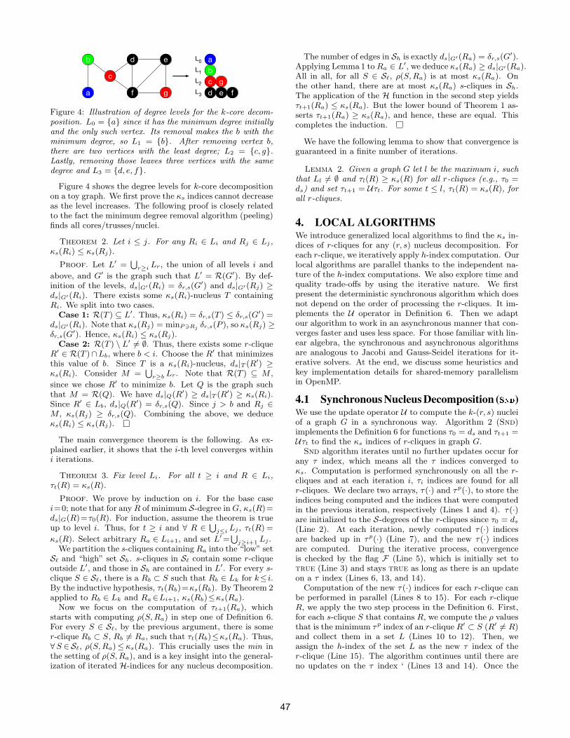
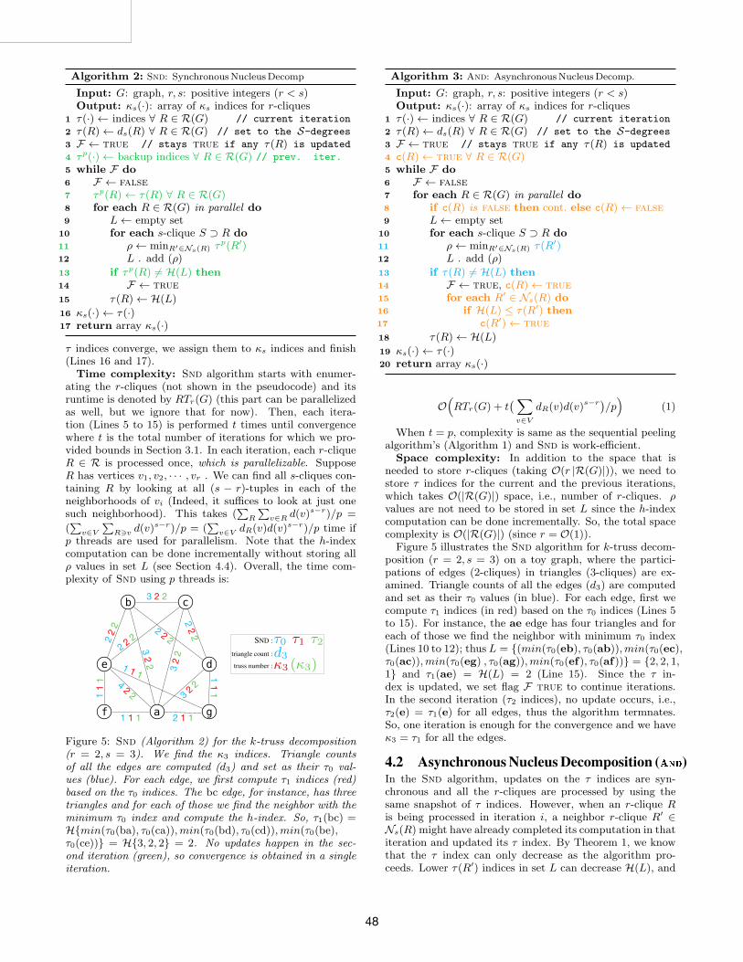
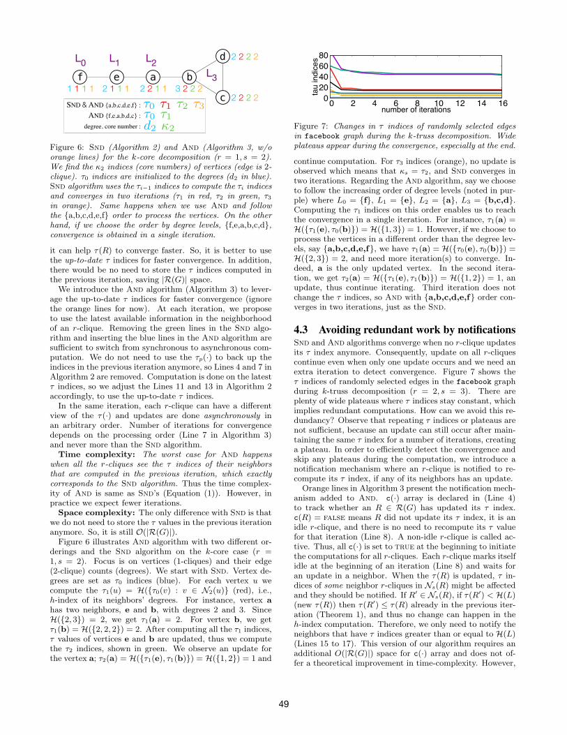
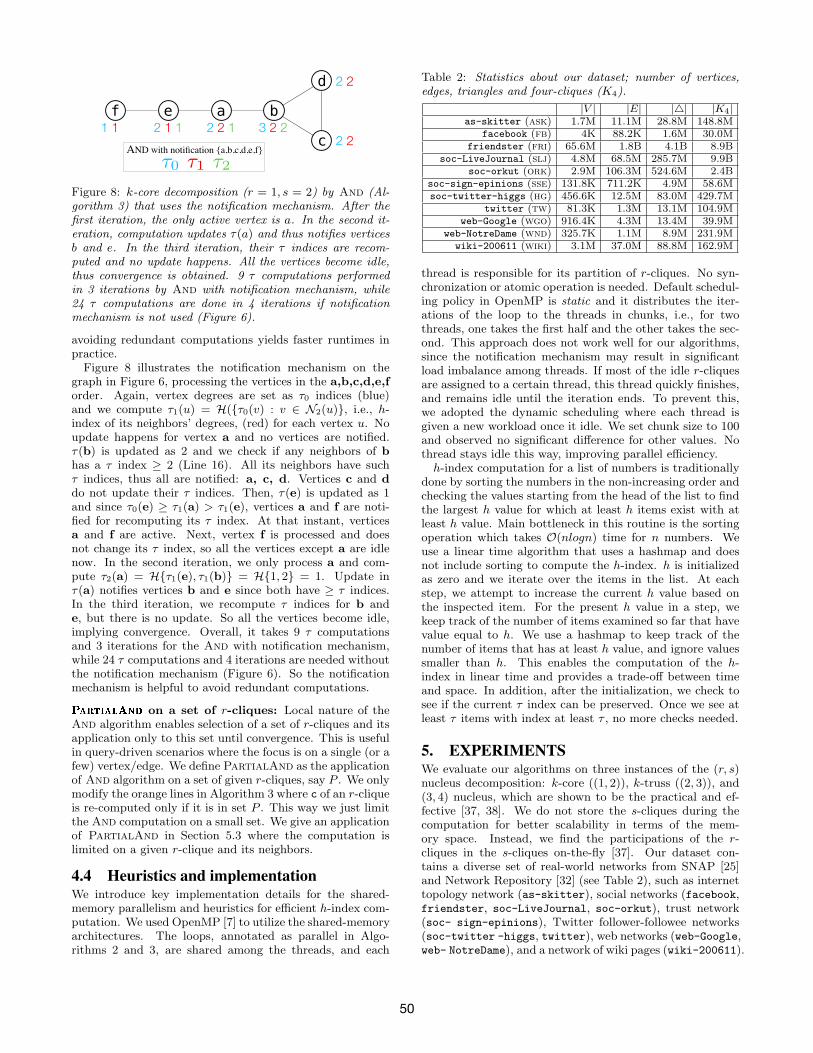


![Core Decomposition and Densest Subgraph in Multilayer …Extracting dense structures from large graphs has emerged as a key graph-mining primitive in a variety of scenarios [28]. Although](https://static.documents.pub/doc/80x56/5edad31a09ac2c67fa685d86/core-decomposition-and-densest-subgraph-in-multilayer-extracting-dense-structures.jpg)
