1

LOCAL ANALYSIS OF FASTENER HOLESUSING THE LINEAR GAP TECHNOLOGY OF

MSC/NASTRANby

John McCullough,

Contract Engineer, Airframe Structures,

Bell Helicopter TEXTRON, Inc., Fort Worth, TX

And

Lance Proctor

Sr. Technical Representative,

Aerospace Business Unit, Grapevine, TX

The MacNeal-Schwendler Corporation

Presented at the 1999 MSC Aerospace Users’ Conference

Abstract (Review Copy 16-Apr-99):Local analysis of bearing stresses at fastener locations in helicopters provides the information needed toprevent cracks which could lead to catastrophic failures. The analysis has typically been done usingnonlinear methods, which can lead to excessive run times. The “linear gap” technology introduced inMSC/NASTRAN V70.5 linear static solution (SOL 101) can be used to assess the bearing stress regions ofthe skin in an efficient manner. This paper will introduce the methodology and strategies of implementinglinear gaps to solve bearing stress problems.

2

Introduction:MSC/NASTRAN Version 70.5 introduced a new method for analyzing gaps in a linearstatic (SOL 101) solution. The linear gap can be thought of as a contact element in itssimplest form: either open or closed with no friction. This paper will describe the theorybehind the linear gap technology, introduce an MSC/PATRAN interface to efficientlygenerate the gaps, and finally, apply the new technology to real world engineeringproblems. The linear gap technology provides an alternative to the nonlinear gapelements in SOL 106.

With the advent of SOL 101 linear gaps, we can redefine the usefulness ofMSC/NASTRAN for aircraft structural analysis. Although improvements in computerhardware performance continue at a steady pace, reducing solve times and allowing moreDOF’s than ever before, the implementation remains largely unchanged. In the aircraftstructures community, we regularly take advantage of our access to significantly fastercomputers to build and solve entire airframe models with enough detail to resolve truehot spots.

Most airframe structure tends to include skins, spars, ribs, frames, bulkheads, stringers,longerons, as well as the fittings that tie various parts together. These parts usuallyconsist of thin plate or sheet metal, or a graphite laminate. They often have large panels,webs or bays which require discreet or generalized stiffening to resist buckling orcrippling. As in all models of structural components, generating the proper boundaryconditions can be critical to the success of the analysis.

Previous efforts to determine the true heel-toe interaction of structural models haveincluded “temp rod” solutions or nonlinear solutions with actual GAP elements. The“temp rod” solution requires that the analyst use rods or springs in a linear solution,turning off those in tension while keeping those in compression, iterating untilequilibrium is achieved. This is often a time consuming method, but can produce goodresults. Using gap elements in nonlinear has its own set of challenges, not the least ofwhich are debugging and extended solve times.

The SOL 101 linear gap method essentially combines the “temp rod” solution with anonlinear gap solution. The linear gaps combine the best of both analysis approaches withfar fewer headaches and significantly less solve time. Essentially, this tool accomplisheswhat the “temp rod” method does, except that MPC’s are employed instead of rods orsprings, and the CLOSE/OPEN iterations are performed automatically.Therefore, we should keep in mind that, at best, this is still a linear solution, but onewhich, if used properly, can provide realistic part to part interface loads or boundaryconditions.

The example in Section 4 illustrates how the linear gaps can be used in a large structuralassembly to determine fastener loads and heel-toe contact forces for every structuralcomponent in the model. The results of the heel-toe contact can be used to construct aFree Body Diagram of any part in the assembly using MSC/PATRAN. These forces canthen be used as applied loads for a sub model that can be solved as a stand alone model

3

containing the necessary refinements to produce accurate local stresses at the edges of aloaded fastener hole.

1. TheoryLinear gaps are implemented in SOL 101 by using explicit Multi-Point Constraints(MPCs) to define the gaps. Because MPCs are used, there is no gap stiffness; adjacentgrids are either “welded” or ‘free” in the user specified degrees of freedom. The lineargaps provide for contact, or compressive, forces only. Because of the implementation,friction is not available, but a large class of problems can be solved efficiently. TheMPCs are satisfied by an iterative technique that is built into SOL 101. The solutionconverges when there is no penetration of MPCs (i.e. gap deflection >=0.0) and there areno tensile forces.

DEFINING THE MPC.

Consider 2 Grids A, and B which are separated by an initial opening of 0.05 inches in theX direction:

Figure 1. Grids A and B used to define MPC.

The gap displacement is defined as:

Uxgap = UxA - UxB + Uxinit (Eq 1)

Rearranging terms to fit an MPC equation:

Uxgap - UxA + UxB - Uxinit = 0 (Eq 2)

Since the gap displacement is iterated on in the MSC/NASTRAN R-set, it cannot bedependant, and the initial gap opening will be in the S-set; either UxA , or UxB must bedependant. We will choose UxB to be dependent for this paper. Rewriting once more,putting the dependant term first:

UxB - UxA + Uxgap - Uxinit = 0 (Eq 3)

4

Assigning Grid A = 84 and Grid B = 21, the MSC/NASTRAN bulk data entries fordefining this gap are:

$gap between grid 84 dof 1 and grid 21 dof 1 init opening = 0.05SPOINT 10001 10002SUPORT 10001 0SPC 101106 10002 0 0.050000MPC 101106 21 1 1. 84 1 -1. 10001 0 1. 10002 0 -1.

Listing 1.

• SPOINT 10001 is used to define the gap opening.

• The SUPORT entry places SPOINT 10001 in the MSC/NASTRAN R-set.

• SPOINT 10002 is used as the initial gap dof

• The SPC entry for SPOINT 10002 defines the initial opening of .05 inches.

• The MPC is written in the form of Equation 3.

Related MSC/NASTRAN Bulk Data entries are:

• PARAM, CDITER (integer) maximum number of iterations to determine open/closed

• PARAM, CDPRT (yes/no) print iteration history of constraint violations

• PARAM, CDPCH(yes/no) punches DMIG,CDSHUT entries for final solutions

• DMIG, CDSHUT Input vector of initial open/closed state of gaps (default=all closed)

5

2. MSC/PATRAN Interface

An MSC/PATRAN PCL utility was written as part of this paper to aid the engineer indefining the gaps. Details of using the MSC/PATRAN interface are included in AppendixA. All features of the linear gap element creation are supported. However, sinceMSC/PATRAN does not currently support SPOINTs, a minor edit of theMSC/NASTRAN file is required. Of particular note is the “proximity” option which canbe used to generate multiple linear gap MPC’s quickly. This option allows the user togenerate linear gaps for all nodes in a list which lie within a user specified distance,relieving the tedium of generating individual gaps.

Figure 2. Sample display of linear gaps in MSC/PATRAN

Figure 2 shows a sample of how the linear gaps can be shown with the interface. Notethat the initial opening is shown, an “S” or an “O” indicates initially shut or open, andarrows show the direction of the gap. These useful display items can be turned on or offdepending on the users needs.

3. Simple Model

Consider two cantilevered plates with a .05 inch initial space between them. The platesare 10.0 inches long, 1.0 inches wide and .10 inches thick with generic Aluminumproperties. Only the top plate is loaded with 15 pounds at the mid-span, and 15 pounds atthe end. The model is meshed with 0.5 inch square CQUAD4 elements. TheMSC/PATRAN interface was used to generate linear gaps between the plates. The initialopening was set to 0.05 inches, and the gaps directly beneath the loads were assumed tobe initially closed, all others were assumed to be initially open.

6

Figure 3. Cantilevered Plate Example— 2 Plates Separated by .05” Gap

MSC/NASTRAN solved this problem with 10 iterations. MSC/PATRAN can be used tographically review the results. The MPC forces and displacements are shown in Figure 4.The results are as expected: the gaps under the far end are all closed, the gaps at mid-spanindicate a parabolic type distribution caused by Poisson’s effects. Review of the centergaps indicates that a more refined mesh may be necessary in this area, but for thepurposes of a demonstration model, no further analysis was performed. This is also alarge deformation problem, but this was ignored for the sake of demonstration.

Figure 4. Cantilevered Plate Results

7

4. Wing Torque Box Assembly Model

The BA609 is a commercial version of the V22 Tiltrotor military aircraft. Figure 5shows pictures of the V22 and a simulated wing torque box section of the BA609. Toavoid revealing any proprietary data associated with a Bell Helicopter TEXTRONproduct, the torque box assembly model was generated using geometry that resembles theBA609 wing. It should be noted that the procedure outlined in this paper was used on theactual BA609 wing.

Figure 5. V22 Photos; Simulated FEM of Single Cell Wing Torque Box

8

The simulated torque box wing consists of:• A forward C-Section spar, flanged aft, and discontinuous at the kick plane• An aft C-Section spar, flanged forward, and discontinuous at the kick plane• An upper and lower skin which are continuous across the kick plane

• Ribs at the kick plane which are tied directly into the upper and lower skins aswell as into the webs of the splice fittings

• Forward and aft splice fittings at each kick plane which are just inside the torquebox

• Forward and aft load fittings at each kick plane which are fastened to the spars

Note that the load fittings and splice fittings work together to splice the forward and aftspars across the kick planes. The LH forward and aft load fittings react vertical as well aslateral loads while the RH forward and aft load fittings react vertical loads only. Allfore/aft drag loads are reacted along the line of nodes connecting the lower skin to thekick plane ribs. All fasteners were represented as bar elements with propertiesdetermined by the stiffness and geometry of each fastener and plate stack-up.

In contrast to a typical composite wing, the simulated wing torque box components wererepresented as monolithic plates, using 0.100 inch thick aluminum. Stiffeners andmaterial thickness variations normally present in any real wing structure were notincluded to maintain simplicity.

Linear gaps (lin-gaps) for SOL 101 were placed between all sets of aligned nodes whichlie adjacent to any fastener to characterize heel-toe interactions at the fastener locations.

Model Summary:

The simulated wing model contains 26,124 elements (plates and bars), 25687 nodes(154122 DOF), 2 RBE2’s to introduce applied forces at the wing tips, and 3368 lin-gaps.Loadcase 1003 is comprised of a symmetric shear of Fz = +5000lb and symmetricmoment of Mx = -15000 in-lb applied to each wing tip. The model was solved on an IBMRS6000 model 595 in approximately 70 CPU minutes. There were a total of 7 iterationsrequired to resolve the 3368 lin-gaps.

9

Model Details:

The purpose of the large simulated wing torque box model is to approximate elastic wingdeflection as closely as possible without the overhead of nonlinear solutions. To this end,sufficient detail of the mechanically fastened joints was included, while less detail of thelarge spans between joints was provided. This reduces the overall DOF’s and assumesthat a more coarse mesh will not adversely affect the quality of the joint loads. In thisexample, every structural fastener in the torque box assembly was represented and lin-gaps were included at each set of adjacent nodes to attempt to capture any heel-toe forcesneeded to carry moment through the joint. In fact, to emphasize the presence of the lin-gaps, all spar flange to skin joints were represented with a single row of .25 dia fasteners,with a parallel row of contact elements .5 inches fwd and .5 inches aft of the fasteners.Although this is an unconventional joint configuration for modern aircraft, it hasadequate shear capability, and the lin-gaps provide the very real moment capability sucha joint would possess. If significant out-of-plane loads were applied to this model, such asair pressures or fuel pressures, the heel-toe contact forces in these joints would be moresignificant.

Figure 6. Spar Splice Joint With and Without Linear Gaps

As it is, the bar elements which represent the fasteners do carry some moment, and thecontact forces which were produced at some of the lin-gaps were due to the linearwarping caused by load path eccentricity. Note that the nodes of all plate elements wereplaced at the proper centroid, one part offset from the next by a distance equal to (t1 + t2)/2 .

10

Data Recovery:

Once the simulated wing torque box model was solved successfully and the resultsscrutinized to a level that produced a reasonable level of confidence, additional loadcasescould be run. Since the detail of this model lies in the mechanical joints, little informationof value can necessarily be gleaned from the large unsupported spans of the majorstructural components. It is the interface loads themselves that are of value. A datarecovery set of all nodes which are connected to any bar elements representing structuralfasteners and any of the lin-gaps in the model was generated. Grid Point Force(GPFORCE) output, written to an XDB file, was then requested for this node set for allloadcases which were subsequently solved. Although solving this model is a significantcomputational task, the only critical output are these GPFORCEs, which are contained ina relatively small .XDB data file. This data can thus be maintained “online” indefinitelyfor use in other applications.

Application of the GPFORCEs:

The first application of the wing model results is simply to use the fastener freebodyforces to perform classical bearing bypass analysis. A simple max/min sort of thesefastener loads for each unique joint configuration can be employed to obtain the criticalbearing margins of safety.

An important distinction should be made between these fastener loads and those obtainedthrough traditional methods. The inclusion of lin-gaps to capture heel-toe forces whichcouple out joint moments has the benefit of calculating the associated out of plane forcesat the fastener. The analysis of a given fastener can thus be more comprehensive byincluding “pull through” loads along with the shear loads. Fastener pull through is oftentreated as a secondary load, and traditional methods of approximating this out of planeforce are tedious and conservative.

An added feature of this first application of the GPFORCEs has to do with the MaterialReview (MR) process. The MR engineer often has to decide whether a part or assemblycan or should be repaired, or simply used as is. Critical loads for parts under review areusually available through either the stress report or at least in the analyst’s stress notes.While this information can be sufficient to make a rough assessment, knowledge of thecritical loads for a given fastener could save considerable time and effort. Examples ofthis might include repairs with oversized fasteners which end up with short edge distance,or evaluating the effect of eliminating a given fastener altogether.

The second application is to perform an eigenvalue (SOL 105) or a nonlinear (SOL 106)analysis of one of the structural regions which has a large enough span to be stabilitycritical. This requires that a freebody for the component be produced for all loadcaseswhich are determined to be reasonable candidates for stability analysis.

11

A stand alone sub model of the component to be checked must be created. This modelshould be based upon the representation of that part found in the assembly model, sinceproper loading requires that the interface nodes match up to those from which thefreebodies were produced. It is certainly possible to create a new model for this purposethat would maintain the interface load node ID’s, but it should not be necessary.

In either case, the sub model of this component must have sufficient resolution in theregion considered stability critical to allow MSC/NASTRAN to adequately predictbuckling mode shapes. If refinement is required, care must be taken to avoid changing thefreebody load interfaces to prevent improper loading.

Finally, in utilizing this second application of the GPFORCEs, it must be clear that sincethe interface loads have been calculated using a linear model, the part represented by thesub model must NOT be allowed to redistribute its applied loads following an elasticinstability. Doing so violates the assumption of linearity which determined the appliedloads. Therefore, this method is an excellent way to CHECK stability of a component ona local level, provided that the results of this analysis support the criteria that the part inquestion remain buckling resistant up to the load limits, including your safety factor.

The third application of the GPFORCEs from the generic wing assembly model is similarto the second. The goal, in this case, is to apply freebody forces for a given component toa sub model of that part as applied loads to capture local stresses at a fastener hole whichhas been locally refined for this purpose. Again it is best, but not absolutely necessary, tostart with the part representation found in the assembly model and work from there.

While the lin-gaps were employed at the outset to better represent part interaction at allthe major joints, detail around a given bolt was not considered. The lin-gaps are usedagain, however, in this third application, as a means to distribute fastener bearing forcesof the bolt shank against the hole in the plate of the part under examination.

The first step in this process is to determine which fasteners in a given part merit thislevel of analysis. In this example, the Forward LH Load Fitting of the generic wing wasfound to be an excellent part, with several fasteners standing out with higher bearing andbypass stresses than most of their neighbors. Figure 7 shows the fitting with theassociated freebody loads. A series of “postage stamp” very fine grid models (submodels) of fastener/hole was generated for various diameters and ID ranges. Forexample,

• ¼ inch diameter 004,104,204,304,404,504,604,704,804,904• 5/16 inch diameter 005,105,205,305,405,505,605,705,805,905• 3/8 inch diameter 006,106,206,306,406,506,606,706,806,906

12

Figure 7. Forward Left Hand Load Fitting Freebody Resultant Forces

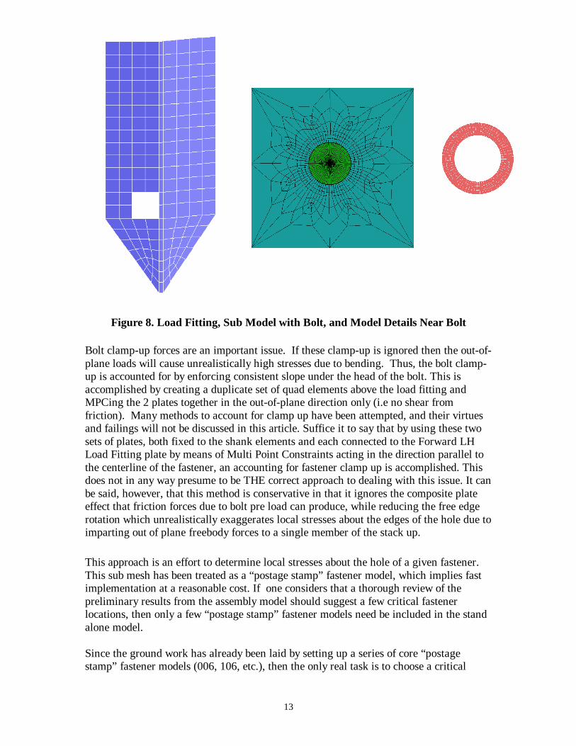
Figure xx shows a plot of the original load fitting with the four quads surrounding thecritical fastener removed and a “postage stamp” representation of the bolt andsurrounding structure to the right. This submodel includes the 006 location describedabove. The ring of 3 rows of quad elements is the plate of the Forward LH Load Fittingunder the head of the most critical fastener in the part. The inner diameter is actually themaximum hole diameter as prescribed by the hole preparation specification associatedwith this fastener. The outer diameter is the maximum diameter of the head of thisfastener. The circle has been segmented into 72 units, a 5 degree arc from the fastenercenterline to each element face. The remaining elements of this postage stamp fastenermodel are in line with this pattern.

The diameter of the shank is the minimum value shown in the fastener specification.Although there is a visible gap shown in this plot, the lin-gaps that are used to connectthese parts have been assigned an initial value of 0.000 inches, which suggests that thefastener and the hole are in intimate mathematical contact.

XY

Z

210

6238

6

8

8

4

11199

295

295

310

314

399

470

13103

99

108

281

174

383

280

9

3

4

4

23

374

4948

9

175

3337

187

307

6

83211

11

93203

2

31177

251

10

49193

232

9 18

XY

Z

Freebody Loads for SC1003 :LC 1003;A3:StaticSubcase -- (4.3)

13

Figure 8. Load Fitting, Sub Model with Bolt, and Model Details Near Bolt

Bolt clamp-up forces are an important issue. If these clamp-up is ignored then the out-of-plane loads will cause unrealistically high stresses due to bending. Thus, the bolt clamp-up is accounted for by enforcing consistent slope under the head of the bolt. This isaccomplished by creating a duplicate set of quad elements above the load fitting andMPCing the 2 plates together in the out-of-plane direction only (i.e no shear fromfriction). Many methods to account for clamp up have been attempted, and their virtuesand failings will not be discussed in this article. Suffice it to say that by using these twosets of plates, both fixed to the shank elements and each connected to the Forward LHLoad Fitting plate by means of Multi Point Constraints acting in the direction parallel tothe centerline of the fastener, an accounting for fastener clamp up is accomplished. Thisdoes not in any way presume to be THE correct approach to dealing with this issue. It canbe said, however, that this method is conservative in that it ignores the composite plateeffect that friction forces due to bolt pre load can produce, while reducing the free edgerotation which unrealistically exaggerates local stresses about the edges of the hole due toimparting out of plane freebody forces to a single member of the stack up.

This approach is an effort to determine local stresses about the hole of a given fastener.This sub mesh has been treated as a “postage stamp” fastener model, which implies fastimplementation at a reasonable cost. If one considers that a thorough review of thepreliminary results from the assembly model should suggest a few critical fastenerlocations, then only a few “postage stamp” fastener models need be included in the standalone model.

Since the ground work has already been laid by setting up a series of core “postagestamp” fastener models (006, 106, etc.), then the only real task is to choose a critical

14

fastener location or two, hang one of the core models in place, use your preprocessor tohelp generate a transition mesh, and equivalence the shared grids. Along with the core“postage stamp” fastener models should be an associated series of lin-gap .BDF fileswhich contain all of the MPC, SUPORT, and SPOINT cards necessary to accommodatethe fastener to plate interaction. In terms of efficiency, these “postage stamp” fastenermodels contain fewer than 1000 elements and should not significantly increase thesolution time, provided too many are not attempted at one time.

Since the applied loads are always in balance, and the original mesh density of thesefittings was not overly coarse, the desire to check many or all of the fasteners for localstresses can easily be accomplished by creating several versions of the stand alone model,each perhaps containing a different zone or cluster of “postage stamp” fastener models.Finally, due to the fact that the applied forces used to load up the stand alone model willnever be perfectly in balance, even though they were produced using freebodies, it isrecommended that several CBUSH translational springs with small spring rates (toground) be tied to the extreme corner grids of the part to prevent “drift”. In addition, arotational CBUSH spring to ground with small spring rate must be included at each boltcenter grid of every “postage stamp” fastener model in the stand-alone model to preventit from spinning about the fastener centerline.

RESULTS

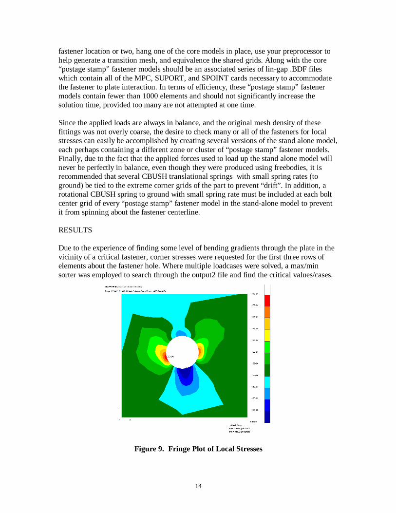
Due to the experience of finding some level of bending gradients through the plate in thevicinity of a critical fastener, corner stresses were requested for the first three rows ofelements about the fastener hole. Where multiple loadcases were solved, a max/minsorter was employed to search through the output2 file and find the critical values/cases.

Figure 9. Fringe Plot of Local Stresses

15

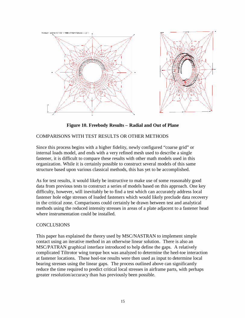
Figure 10. Freebody Results – Radial and Out of Plane

COMPARISONS WITH TEST RESULTS OR OTHER METHODS

Since this process begins with a higher fidelity, newly configured “coarse grid” orinternal loads model, and ends with a very refined mesh used to describe a singlefastener, it is difficult to compare these results with other math models used in thisorganization. While it is certainly possible to construct several models of this samestructure based upon various classical methods, this has yet to be accomplished.

As for test results, it would likely be instructive to make use of some reasonably gooddata from previous tests to construct a series of models based on this approach. One keydifficulty, however, will inevitably be to find a test which can accurately address localfastener hole edge stresses of loaded fasteners which would likely preclude data recoveryin the critical zone. Comparisons could certainly be drawn between test and analyticalmethods using the reduced intensity stresses in areas of a plate adjacent to a fastener headwhere instrumentation could be installed.

CONCLUSIONS

This paper has explained the theory used by MSC/NASTRAN to implement simplecontact using an iterative method in an otherwise linear solution. There is also anMSC/PATRAN graphical interface introduced to help define the gaps. A relativelycomplicated Tiltrotor wing torque box was analyzed to determine the heel-toe interactionat fastener locations. These heel-toe results were then used as input to determine localbearing stresses using the linear gaps. The process outlined above can significantlyreduce the time required to predict critical local stresses in airframe parts, with perhapsgreater resolution/accuracy than has previously been possible.

16

A. Appendix A – Details of MSC/PATRAN Linear Gap Interface

The purpose of the MSC/PATRAN Linear Gap Interface is to fully support theMSC/NASTRAN V70.5 linear gaps in SOL 101. The supported features includeautomatic generation of gaps, parameters and DMIG entries necessary forMSC/NASTRAN.

Primary Features:• Specify initial gap— Several options

• Automatically calculated based on nodal distance• Automatically calculated nodal distance projected into displacement c.s.• Explicitly defined (user input)

• Specify initial condition (shut/open)• Graphically identify displacement (analysis) dof direction to ensure proper definition• Generate graphical representation of gaps

• Identify independent vs. dependent dof• Draw a line between gap nodes

• Automatically reorder MPC equation if MSC/NASTRAN set conflicts are detected(i.e. dependent dof can only be specified 1 time, dependent dof cannot be spc’d)

• Automatically generate gaps for nodes within a user specified proximity• Delete unwanted gaps• Graphical verifications

• Initial conditions (open/shut)• Initial gap opening• Independent/dependent dof colors/marker identification• Displacement vector to show closing direction of gaps

• Write bulk data entries for PARAMeters, SUPORTs, SPCs, MPCs, SPOINTS, andDMIGs

• Read bulk data entries associated with linear gaps.

Creating Gaps

There are 2 methods to create the linear gaps: individually selecting nodes and choosing agroup of nodes to match based on proximity (model distance.) The creation form isshown for both methods:

17

18

Several valuable checks are performed when creating a gap. MSC/NASTRAN setdefinitions are enforced when writing the MPC equation. Specifically, theMSC/PATRAN database is searched for dof which are part of the S-set and M-set. TheS-set is the Single Point Constraint (SPC) set, which cannot be specified as a dependentdof. The MSC/PATRAN database is searched for any nodes which have displacementconstraints (S-set), and the MPC equation will be automatically rewritten if S-set dof ischosen as dependent. A form is used to “filter” the displacement constraints used in thischeck. By default all displacements constraints will be searched. The MPC equations onthe MSC/PATRAN database are also interrogated to ensure that a dependant dof isn’tspecified more than 1 time.

CREATION by SELECT NODES:

By default, the Node 1 will be the independent node in the MPC equation, and theequation will be written in the format shown in EQ 3. Note that the user must determinewhich node to select first.

• For non-coincident nodes, Node 1 should be the node which has the higher coordinatevalue in the dof selected. (I.e. choose node with coordinates [1.01, 0.0, 0.0] as Node1, and [1.00, 0.0, 0.0] as Node 2 for a gap in the X direction). There is no check bythe program to ensure compliance; the equation will be written as EQ 3.

19

• For coincident nodes, Node 1 should belong to the object or model component whichis “above” the other object. An example of this would be a table sitting on the floor.Assume that the Z-axis is pointing up from the floor. Then the coincident nodes atthe table leg/floor interface should be chosen with Node 1 belonging to the table legand Node 2 belonging to the floor.

CREATION by PROXIMITY

A far more valuable tool provided by the graphical interface is creation by proximity.Here, a group of nodes is compared to another group of nodes. If the nodes fall within aspecified tolerance (10 times model tolerance), then a gap is created between them. Theprogram will automatically determine the MPC equation based on the nodal coordinates.If two nodes are coincident, then Node 1 will be based on the “Higher” or “Lower”toggle above the proximity threshold input box. The proximity method is preferred forcreating linear gaps.

CREATION: Gap Input Method

The creation form allows several methods of determining the initial gap opening. “NodalDistance” will calculate the magnitude of the distance between the two nodes for use inthe initial opening. This is useful for models with solid interfaces, but should be usedwith caution for plate or beam interfaces because the actual gap may be different than thenodal distance. The “Nodal Distance” “Option” is either Magnitude, or a projection ofthe magnitude into one of the analysis coordinate systems of one of the nodes. “EnterValue” allows the user to specify the initial gap distance.

CREATION: Initial Position

The initial position can be specified as “Shut” or “Open.” The MSC/NASTRAN defaultis “Shut” for all gaps. If any of the gaps are created with an initial “Open,” then theappropriate DMIG CDSHUT entries will be written to the MSC/NASTRAN input file.Careful selection of initial position can greatly improve the solution iteration time.

CREATION: Node 1 DOF and Node 2 DOF

Since an explicit MPC is written for each linear gap, the dof must be specified to definethe MPC properly. As an aid to the user, an arrow is drawn in the analysis coordinatesystem (displacement coordinate system) of the node when it is selected. The analysiscoordinate system direction is calculated using the analysis coordinate frame of the node.The graphical interface will automatically resolve any coordinate system transformationsand display the appropriate arrow. Rectangular, cylindrical, and spherical coordinatesystems are all displayed appropriately. A toggle is provided if the user doesn’t wish tosee the displacement coordinate systems when selecting nodes. The “Auto Execute” willautomatically toggle between the Node 1 and Node 2 selections.

20

CREATION: Delete Last Gap

Since there is no “Undo” for the creation, a “Delete Last Gap” button is included on theform. This will delete the last gap entry. This can be used multiple times to delete asmany gaps as necessary, always deleting the most recently created gap. There is anoption to delete gaps which can be used for more extensive deletion.

CREATION: Proximity Threshold

This is explained in “CREATION by PROXIMITY” above.

Displaying Gaps

The “Display” option allows the user to modify the display attributes of the gap. Thisform requires no further explanation.

21

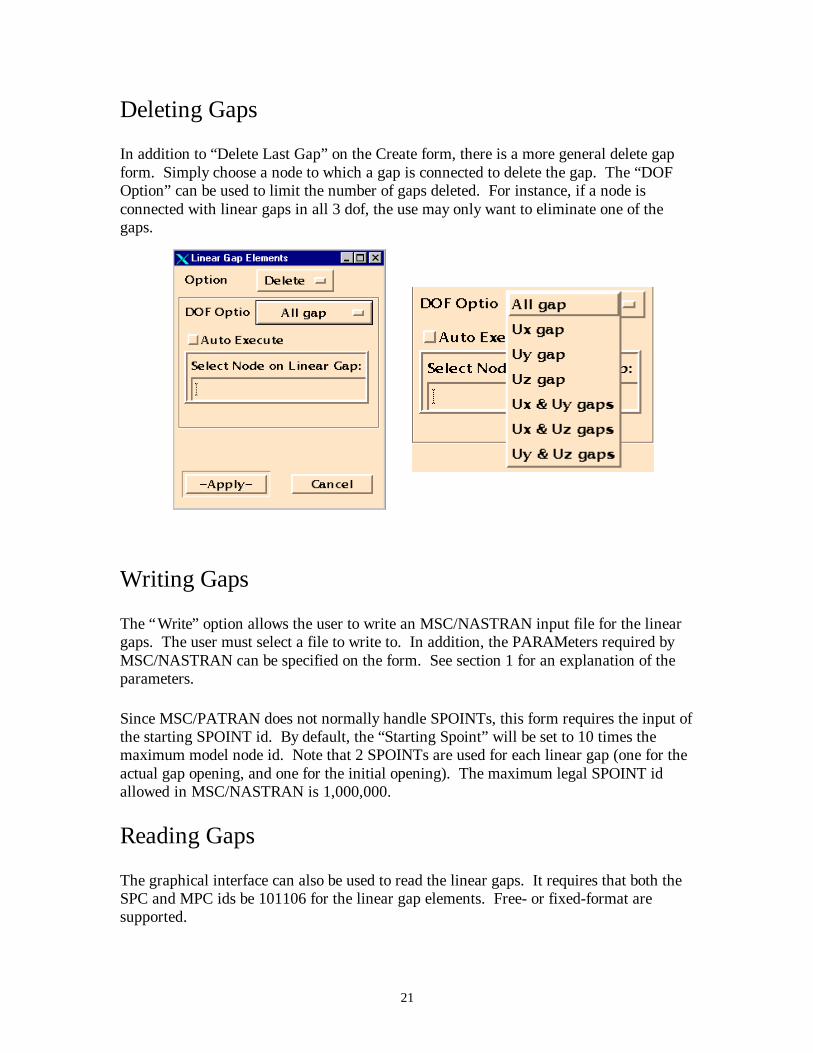
Deleting Gaps

In addition to “Delete Last Gap” on the Create form, there is a more general delete gapform. Simply choose a node to which a gap is connected to delete the gap. The “DOFOption” can be used to limit the number of gaps deleted. For instance, if a node isconnected with linear gaps in all 3 dof, the use may only want to eliminate one of thegaps.

Writing Gaps

The “Write” option allows the user to write an MSC/NASTRAN input file for the lineargaps. The user must select a file to write to. In addition, the PARAMeters required byMSC/NASTRAN can be specified on the form. See section 1 for an explanation of theparameters.

Since MSC/PATRAN does not normally handle SPOINTs, this form requires the input ofthe starting SPOINT id. By default, the “Starting Spoint” will be set to 10 times themaximum model node id. Note that 2 SPOINTs are used for each linear gap (one for theactual gap opening, and one for the initial opening). The maximum legal SPOINT idallowed in MSC/NASTRAN is 1,000,000.

Reading Gaps

The graphical interface can also be used to read the linear gaps. It requires that both theSPC and MPC ids be 101106 for the linear gap elements. Free- or fixed-format aresupported.

22

Verifying Gaps

To verify the gaps, a displacement result case is created. This result case will create anegative unit (-1.0) displacement for the node which will move in the “closing” directionof the gap. All other nodes have no displacement. The user can then use the normalMSC/PATRAN “Results” to plot the closing direction of the gap to provide a visualverification of the gap closing directions. See also “Displaying Gaps” above.

23

Modifying the MSC/NASTRAN Input Deck

After creating, verifying, and writing the linear gaps, an MSC/NASTRAN input deck canbe created with MSC/PATRAN as with an ordinary static analysis. Be sure to create ananalysis deck only and don’t submit the run until the following edits to the input file areperformed:

1) In the case control section: add “MPC = 101106” prior to the 1st SUBCASE

2) After “BEGIN BULK” add “INLCUDE ‘lin_gap_filename.dat’”

3) Modify the “SPCADD” entry to include spc set 101106

A sample is shown here, the modifications are denoted in bold:……MAXLINES = 999999999$ Direct Text Input for Global Case Control Datampc=101106SUBCASE 1$ Subcase name : Default SUBTITLE=Default SPC = 2……BEGIN BULKinclude 'plate_gaps.dat'PARAM POST -1PARAM PATVER 3.……$ Loads for Load Case : DefaultSPCADD 2 1 101106……

Usage Notes

• The preferred way to generate the gaps is with the “Proximity” option.

• The user is urged to use the “Display” and “Verify” forms to determine if the gapswere generated correctly.

24

• If the user wants to modify a gap, he can simply re-create the gap with the new values(i.e. initial opening or initial position).

• For existing MSC/NASTRAN bulk data files, the model can be read intoMSC/PATRAN and the gaps created and written to another file.

• The user must remember to request MPC FORCES in the case control outputrequests.

• It is strongly recommended to use PARAM CDPCH to generate DMIG CDSHUTentries on the MSC/NASTRAN punch file. These can be used in subsequent analysesas a refined starting point (initial condition).

Limitations

Because MSC/PATRAN does not recognize SPOINTs, the user must modify theMSC/NASTRAN input file. There are precisely 3 modifications which should take theaverage user less than 1 minute to perform. When MSC/PATRAN recognizes SPOINTs,this limitation can be avoided.

The MPC and SPC set ids generated for the linear gaps are each 101106. If, by Murphy’sLaw, the user has an existing input file which uses these set ids, the user will have tomodify the set ids manually. This should be a relatively simple step of performing aglobal replace of 101106 in the file generated by the graphical interface. TheMSC/NASTRAN input file modifications will have to be modified accordingly.