Date post: | 21-Dec-2015 |
Category: |
Documents |
View: | 216 times |
Download: | 0 times |
Local Features and Kernels for Classification of Object Categories
J. Zhang --- QMUL UK (INRIA till July 2005)
with
M. Marszalek and C. Schmid --- INRIA France
S. Lazebnik and J. Ponce --- UIUC USA
Motivation Why?
Describe images, e.g. textures or categories, with sets of sparse featuresHandle object images under significant viewpoint changes Find better kernels
ResultingStronger robustness and higher accuracyBetter kernel evaluation
Outline
Bag of features approach Region extraction, description Signature/histogram Kernels and SVM
Implementation choice evaluation Detectors & descriptors, invariance, kernels Influence of backgrounds
Spatial bag of features Spatial pyramid
Results on Pascal 06 validation data
Image RepresentationSparse: regions from interest points
— Harris-Laplace: H HS, HSR and HA— Laplacian: L LS, LSR and LA— Invariance: S (scale), SR (scale and rotation), and A (affine)
Dense: regions from points on a fixed grid— Multi-scale -- fixed grid (5000 points per image)
Description— SIFT (Lowe, IJCV 2004) and SPIN images (Lazebnik et al, PAMI
2005)
Harris-Laplace
Laplacian
Image signature/HistogramSignature: cluster each image
Earth Movers Distance (EMD) (Rubner et al. IJCV2000)
and
is the ground truth distance; is the flow
Visual words: cluster all training images Histogram-based distances
Euclidean distance distance
histogram intersection any other histogram distances
}...,,1),,{( miwu ii
}...,,1),,{(2 niwuS ii
m
i
n
j ji
m
i
n
j jiji
f
fdSSD
,
,,)2,1(
),( jid ),( jif
}...,,1),,{(1 miwuS ii
m
i iiii wuwuSSD1
221 )]()([
2
1),(
}...,,{1 1 muuS }...,,{2 1 mwwS 2
Kernel-based Classification
Kernelization: Traditional kernel : linear, RBF Extended Gaussian kernel
Resulting : EMD or kernel
Combination: Direct sum
A two-layer SVM classifier: SVM+ kernel SVM + RBF kernel
Classification: SVM Binary SVM (Object prediction) Multi-Class SVM (multi-class classification)
i
iDD
)/1exp(),( 21 DAIIK
2
2
Method Flow Chart
Bag of features + SVM classifer
[Zhang, Marszalek, Lazebnik & Schmid, Workshop CVPR 2006]
Outline
Bag of features approach Region extraction, description Signature/histogram Kernels and SVM
Implementation choice evaluation Detectors & descriptors, invariance, kernels Influence of backgrounds
Spatial bag of features Spatial pyramid
Results on Pascal 06 validation data
Evaluation: Detectors and Descriptors
Channels SIFT SPIN SIFT+SPIN
HS 92.0 ±2.0 83.0 ±1.9 91.4 ±2.1
LS 93.9 ±1.5 88.6 ±2.0 94.3 ±0.9
HS+LS 94.7 ±1.2 89.5 ±1.4 94.3 ±1.1
Xerox7: 10 fold cross validation
LS better than HS – more points
The combination of detectors is the best choice
Lap with SIFT is acceptable with less computational cost
Channels SIFT SPIN SIFT+SPIN
HSR 97.1 ±0.6 93.9 ±1.1 97.4 ±0.6
LSR 97.7 ±0.6 93.9 ±1.0 98.2 ±0.6
HSR+LSR 98.0 ±0.5 96.2 ±0.8 98.3 ±0.5
UIUCTex: 20 training images per class
Evaluation: Invariance
Datasets nScale Invariance Scale and Rotation Affine Invariance
HS LS HS+LS HSR LSR HSR+LSR HA LA HA+LA
UIUCTex 20 89.7±1.6 91.2±1.5 92.2±1.4 97.1±0.6 97.7±0.6 98.0±0.5 97.5±0.6 97.5±0.7 98.0±0.6
Xerox710
fold92.0±2.0 93.9±1.5 94.7±1.2 88.1±2.1 92.4±1.7 92.2±2.3 88.2±2.2 91.3±2.1 91.4±1.8
Best invariance level depends on datasets
Scale invariance is often sufficient for object categories
Affine invariance is rarely an advantage
Evaluation: Kernels
Datasets
Training images
per class
Spares representation
Vocabulary-Histogram Signature
Linear Poly (n=2)
RBF kernel EMD+KNN EMD-kernel
UIUCTex 20 97.0±0.6 84.8±1.6 97.3±0.7 98.1±0.6 95.0±0.8 97.7±0.6
Xerox7 10 fold 79.8±3.0 70.9±2.4 86.2±2.2 89.2±2.1 59.4±4.1 92.4±1.7
EMD and kernel gives the best/comparable results
Higher vocabulary usually gives higher accuracy: gives 93% on Xerox7 when using 1000 instead of 70.
Experimental setting: sig. size: 40 for EMD; number of clusters per class is 10 for kernel
2
2
2
2
Comparison with state-of-the-art
Methods Xerox7 CalTech6
Graz Pascal05Test 1
Pascal 05Test 2
CalTech101
(HS+LS)(SIFT+SPIN)
94.3 97.9 90.0 92.8 74.3 53.9
Others 82.0Csurka.et al. (ICPR
2004)
96.6Csurka.et al (ICPR 2004)
83.7Opelt et al eccv
04
94.6Jurie and Triggs iccv 05
70.5Deselares et
al cvpr 05
43Grauman and
Darrel iccv 05
Results are the mean values of the accuracies
Better reults on 5 datasets and comparable results on Pascal05 test set 1
Influence of Background Questions:
Background correlations?
Do background features make recognition easier?
What kinds of backgrounds are best for training?
Test Bed: PASCAL 05
Protocol:
Use bounding rectangles to separate foreground features (FF) from background features (BF)
Introduce two additional background sets:
Randomly shuffle backgrounds among all images (BF-RAND)
Constant natural scene (BF-CONST)
Conclusions on influence of background
Backgrounds do have correlations with the foreground objects, but adding them does not result in better performance for our method It is usually beneficial to train on a harder training set
Classifier trained on uncluttered or monotonous background tend to overfit
Classifiers trained on harder ones generalize well
Add random background clutter to training data if backgrounds may not be representative of test set
Based on these results, we include the hard examples marked with 0 for training in PASCAL’06
Outline
Bag of features approach Region extraction, description Signature/histogram Kernels and SVM
Implementation choice evaluation Detectors & descriptors, invariance, kernels Influence of backgrounds
Spatial bag of features Spatial pyramid
Results on Pascal 06 validation data
Spatial Pyramid for Bag of Features
Pyramid comparisonA two-layer SVM classifier: first layer: ; second: RBFSpatial pyramid matching kernel [Lazebnik, Schmid & Ponce, CVPR 2006]
2
Spatial Pyramid Matching kernel
Histogram intersection at level l
Spatial pyramid matching kernel – mercer kernel
D
i
ly
lx
ly
lx jHiHHHI
1
))(),(min(),(
L
l
llLL
llL
llL
Ll
II
IIIYXk
11
0
11
0
2
1
2
1
)(2
1),(
PASCAL06 Experimental Settings
Regions: Sparse: HS+LS Dense: Multi-scale, fixed grid, 5000 points per image
Kmeans -- cluster the descriptors of each class separately and then concatenate them, 300 clusters per class3000 visual words for sparse and dense representations.Kernels: kernel, spatial pyramid kernelBag of features: (HS+LS)(SIFT) denoted as HS+LS combined with a two-layer SVM classification strategy .Spatial pyramid
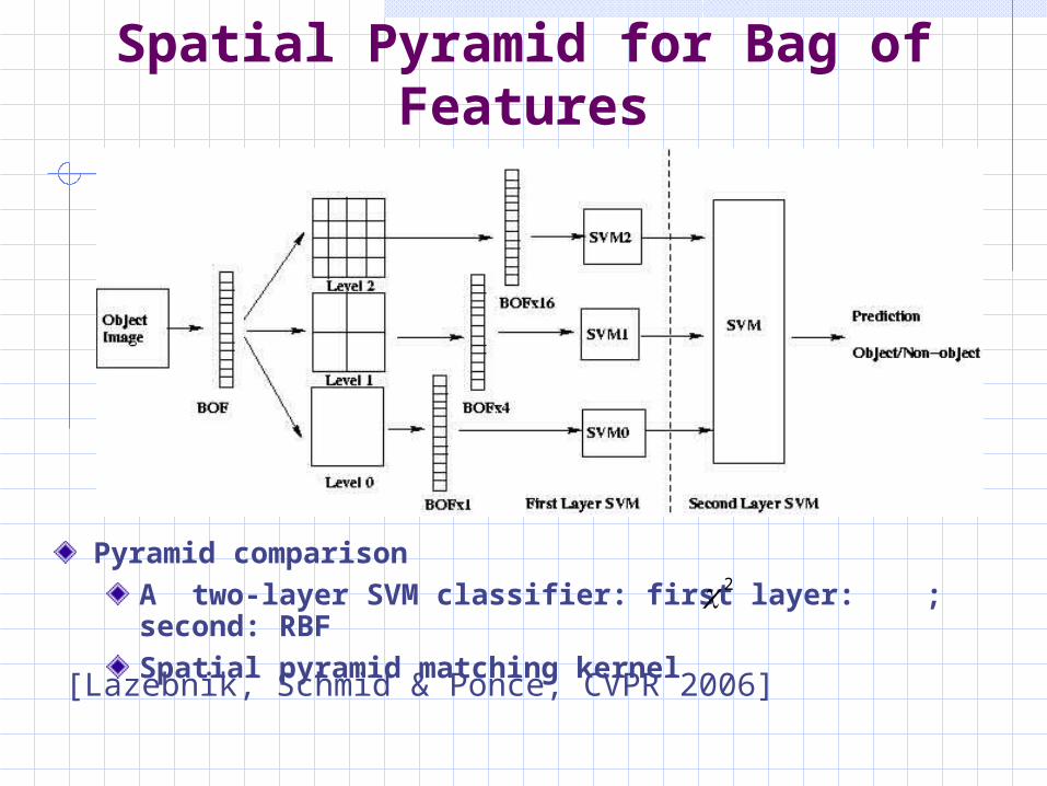
train SVM for each spatial level, and then using the two-layer SVM classification strategy to combine them
spatial pyramid matching kernel. levels up to 2
Classification: binary SVM with output normalized to [0, 1] by (x-min)/(max-min)
2
Methods Summary (HS+LS): the bag of keypoints method with a two-layer SVM classifier(LS)(PMK): Laplacian points with spatial pyramid matching kernel(DS)(PMK): Multi-scale dense points with spatial pyramid matching kernel (DS)(PCh): Multi-scale dense points with a two-layer spatial pyramid SVM(LS)(PCh): Laplacian points with a two-layer spatial pyramid SVM(LS) : Laplacian points with a kernel(HS+LS)(SUM): the bag of keypoints method with a SUM of the distances
2
2
AUC for VOC Validation SetMethods HS+LS (LS)
(PCh)(DS)(PCh)
(LS)(PMK)
(DS)(PMK) LS HS+LS (SUM)
Bicycle 0.904 0.912 0.901 0.909 0.894 0.901 0.906
Bus 0.970 0.967 0.952 0.963 0.949 0.967 0.970
Car 0.955 0.954 0.956 0.950 0.955 0.953 0.956
Cat 0.923 0.921 0.908 0.916 0.902 0.915 0.926
Cow 0.931 0.935 0.925 0.933 0.919 0.931 0.928
Dog 0.865 0.855 0.853 0.848 0.841 0.853 0.861
Horse 0.920 0.929 0.897 0.912 0.874 0.918 0.915
Motorbike
0.935 0.935 0.915 0.924 0.908 0.934 0.937
Person 0.841 0.840 0.815 0.824 0.792 0.840 0.838
Sheep 0.925 0.936 0.925 0.934 0.928 0.931 0.927
Av. 0.917 0.918 0.905 0.911 0.896 0.914 0.916(HS+LS) , (LS)(PCh) the best A two-layer SVM classifier better than spatial pyramid kernel : (LS)(PCh) > (LS)(PMK); DS(PCh) > (DS)(PMK)Spatial information helps a bit (LS)(PCh) >= LS
AUC Measures PMK (Levels 0,1,2)
(LS)(PMK)
200 500 1000
L0 L1 L2 L0 L1 L2 L0 L1 L2
Bicycle 0.802 0.886 0.886 0.834 0.889 0.905 0.882 0.882 0.893
Bus 0.862 0.885 0.907 0.926 0.917 0.929 0.943 0.939 0.948
Car 0.920 0.937 0.943 0.935 0.946 0.949 0.942 0.949 0.953
Cat 0.817 0.867 0.878 0.866 0.893 0.904 0.885 0.902 0.909
Cow 0.833 0.852 0.890 0.887 0.914 0.909 0.910 0.909 0.914
Dog 0.737 0.810 0.810 0.800 0.840 0.847 0.826 0.845 0.838
Horse 0.766 0.860 0.844 0.860 0.873 0.882 0.889 0.877 0.870
Motorbike
0.841 0.835 0.866 0.863 0.897 0.907 0.889 0.901 0.904
Person 0.731 0.757 0.775 0.768 0.791 0.807 0.801 0.799 0.807
Sheep 0.829 0.874 0.894 0.925 0.919 0.923 0.913 0.924 0.926
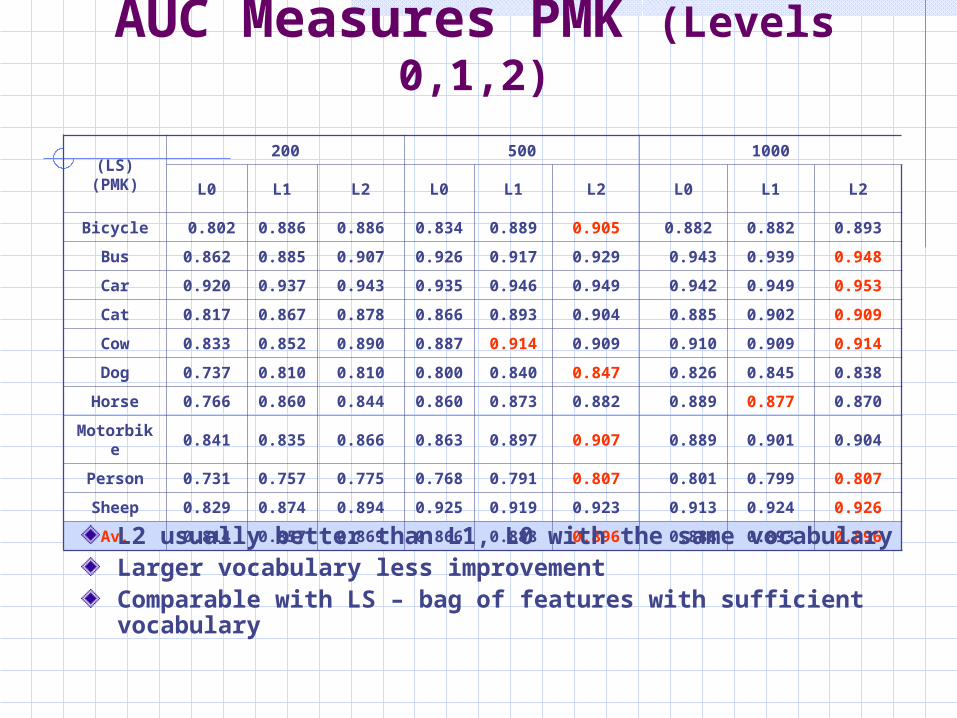
Av. 0.814 0.857 0.869 0.866 0.888 0.896 0.888 0.893 0.896L2 usually better than L1, L0 with the same vocabularyLarger vocabulary less improvementComparable with LS – bag of features with sufficient vocabulary
ConclusionsOur approaches give excellent results -- (HS+LS), (LS)(PCh) the bestSparse (interest points sampling) rep. performs better than dense rep. (4830 vs. 5000) A two-layer spatial SVM classifier gives slightly better results than pyramid matching kernelSpatial constrains help classification, however, perform similarly to bag of features with a sufficient large vocabulary in the context of PASCAL’06