Local Food Prices, SNAP Purchasing Power, and Child Health Erin T. Bronchetti Department of Economics, Swarthmore College [email protected]Garret Christensen Berkeley Institute for Data Science, UC Berkeley [email protected]Hilary W. Hoynes Department of Economics and Public Policy, UC Berkeley [email protected]September 12, 2017 Abstract: The Supplemental Nutrition Assistance Program (SNAP, formerly food stamps) is one of the most important elements of the social safety net. Unlike most other safety net programs, SNAP varies little across states and over time, which creates challenges for quasi-experimental evaluation. Notably, SNAP benefits are fixed across 48 states; but local food prices vary, leading to geographic variation in the real value of SNAP benefits. In this study, we provide the first estimates that leverage variation in the real value of SNAP benefits across markets to examine effects of SNAP on child health. We link panel data on regional food prices to National Health Interview Survey data and use a fixed effects framework to estimate the relationship between local purchasing power of SNAP and children’s health and health care utilization. We find that children in market regions with lower SNAP purchasing power utilize less preventive health care. Lower real SNAP benefits also lead to an increase in school absences. We find no effect on reported health status. * This project was supported with a grant from the University of Kentucky Center for Poverty Research through funding by the U.S. Department of Agriculture, Economic Research Service and the Food and Nutrition Service, Agreement Number 58-5000-3-0066. The opinions and conclusions expressed herein are solely those of the author(s) and should not be construed as representing the opinions or policies of the sponsoring agencies. We thank Krista Ruffini for excellent research assistance.
Transcript
Local Food Prices, SNAP Purchasing Power, and Child Health
Erin T. Bronchetti Department of Economics, Swarthmore College
The Supplemental Nutrition Assistance Program (SNAP, formerly food stamps) is one of the most important elements of the social safety net. Unlike most other safety net programs, SNAP varies little across states and over time, which creates challenges for quasi-experimental evaluation. Notably, SNAP benefits are fixed across 48 states; but local food prices vary, leading to geographic variation in the real value of SNAP benefits. In this study, we provide the first estimates that leverage variation in the real value of SNAP benefits across markets to examine effects of SNAP on child health. We link panel data on regional food prices to National Health Interview Survey data and use a fixed effects framework to estimate the relationship between local purchasing power of SNAP and children’s health and health care utilization. We find that children in market regions with lower SNAP purchasing power utilize less preventive health care. Lower real SNAP benefits also lead to an increase in school absences. We find no effect on reported health status.
* This project was supported with a grant from the University of Kentucky Center for Poverty Research through funding by the U.S. Department of Agriculture, Economic Research Service and the Food and Nutrition Service, Agreement Number 58-5000-3-0066. The opinions and conclusions expressed herein are solely those of the author(s) and should not be construed as representing the opinions or policies of the sponsoring agencies. We thank Krista Ruffini for excellent research assistance.
The Supplemental Nutrition Assistance Program (SNAP, formerly the Food Stamp program)
is the largest food assistance program and one of the largest safety net programs in the United
States.1 SNAP plays a crucial role in reducing poverty for children in the U.S., with only the EITC
(combined with the Child Tax Credit) raising more children above poverty (Renwick and Fox
2016). Eligibility for the program is universal in that it depends only on a family’s income and
assets; in 2015, 1 in 7 Americans received SNAP benefits (Ziliak 2015).
SNAP’s primary goals are to improve food security among low-income households, reduce
hunger, and increase access to a healthful diet.2 The extant literature demonstrates that the
program succeeds in reducing food insecurity among recipient households (see, e.g., Yen et al.
2008; Nord and Golla 2009; Mykerezi and Mills 2010; Ratcliffe, McKernan, and Zhang 2011;
Shaefer and Gutierrez 2011; Schmidt, Shore-Sheppard, and Watson 2016 and the recent review
by Hoynes and Schanzenbach 2016). Nonetheless, rates of food insecurity among SNAP
households remain quite high, raising the question of whether SNAP benefits are adequate to
meet the nutritional needs of recipients (Coleman-Jensen et al. 2014). Indeed, evidence
regarding how SNAP benefits impact recipients’ nutrition is more mixed (see, e.g., Yen (2010);
Gregory et al. (2013)).
Our study provides unique and highly policy-relevant evidence on the impact of variation in
the generosity of SNAP benefit levels on child health. Estimating the causal relationship
1 SNAP benefits paid in 2016 amounted to more than 66 billion dollars. The program has also grown dramatically in the years
since 1996 welfare reform, with benefits paid out almost tripling in real terms over the years in this study (1999-2010). 2 See, for example, the most recently amended authorizing legislation, the Food and Nutrition Act of 2008, available at
between SNAP and health is difficult because SNAP benefits and eligibility rules are legislated at
the federal level and do not vary across states, leaving few opportunities for quasi-experimental
analysis. One set of quasi-experimental studies analyzes the rollout of the food stamp program
across counties in the 1960s and 1970s and finds that food stamps leads to significant
improvements in birth outcomes (Currie and Moretti 2008; Almond, Hoynes, and Schanzenbach
2011) and access to food stamps in early childhood leads to significant improvements in adult
health (Hoynes, Schanzenbach, and Almond 2016). A second set of studies uses recent state
changes in application procedures (e.g. allowing online applications, whether there is a finger
printing requirement) as instruments for SNAP participation (Schmeiser 2012, Gregory and Deb
2015),3 though these state policies had relatively small effects on participation (Ziliak 2015). A
third approach is taken by East (2016), who uses variation in eligibility for SNAP generated by
welfare reform legislation in the 1990s, and finds that SNAP in early childhood leads to
improvements in health status at ages 6-16. None of these studies, however, is able to shed
light on how changes to legislated SNAP benefit levels might impact health outcomes.
Our approach leverages plausibly exogenous geographic variation in the real value of SNAP
benefits to identify the effects of variation in SNAP generosity on health for a sample of children
in SNAP households. Importantly, the SNAP benefit formula is fixed across the 48 states
(benefits are higher in Alaska and Hawaii) even though the price of food varies significantly
across the country (Todd et al. 2010; Todd, Leibtag, and Penberthy 2011).4 Across the
3 Gregory and Deb (2015) use the Medical Expenditure Panel Survey and state policy variables and find that SNAP participants
have fewer sick days and fewer doctor’s visits, but more checkup visits. 4 Studying data from the Quarterly Food at Home Price Database (QFAHPD), the authors find that regional food prices vary
from 70 to 90 percent of the national average at the low end to 120 to 140 percent at the high end.
3
continental U.S., maximum benefits vary only with family size. So, in 2016 a family of three
would be eligible for a maximum benefit of $511/month regardless of the local cost of living.
Though SNAP benefits are implicitly adjusted for variation in the cost of living through allowed
deductions (e.g., for housing, and child care) in the calculation of net income, the limited
available evidence indicates these adjustments are not sufficient to equalize real benefits,
particularly in high cost areas (Breen et al. 2011). Gundersen et al. (2011) and the Institute of
Medicine (2013) propose this as an area for future research.
Higher area food prices, and consequently lower SNAP purchasing power, may impact
children’s health by reducing nutrition if households respond by purchasing and consuming
lower quantities of food, or if they purchase less expensive foods of lower nutritional quality.
But lower SNAP purchasing power may also impact health indirectly, with higher food prices
causing households to reduce consumption of other inputs into the health production function,
like health care.
Linking nationally representative data from the 1999-2010 National Health Interview
Surveys (NHIS) to information on regional food prices from the Quarterly Food-at-home Price
Database (QFAHPD), we study the effect of variation in real SNAP benefits (or “SNAP purchasing
power”) on children’s health care utilization and health. Our measure of regional food prices is
the cost of the Thrifty Food Plan (TFP), a nutrition plan that was constructed by the USDA to
represent a nutritious diet at minimal cost and is the basis for maximum legislated SNAP
benefits (i.e., maximum benefits are set to its national average cost). The QFAHPD includes
information on food prices that allows us to construct an estimated TFP price for each of 30
designated “market group” geographic area across the U.S. We relate various child health
4
outcomes to the real value of SNAP benefits (i.e., the ratio of the national SNAP maximum
benefit to the market group-level TFP price faced by a household) in a fixed effects framework
that controls for a number of individual-level and region characteristics (including non-food
prices in the area) and state policy variables. Identification comes from differences across the
30 market areas in trends in the price of the TFP.
Our study contributes to the growing body of evidence on the SNAP program and its effects
in a few key ways. First, we provide new evidence on the relationship between SNAP benefit
generosity and the health and wellbeing of the SNAP population. Our findings consistently
indicate that children in market regions with higher food prices (lower purchasing power of
SNAP) utilize less preventive/ambulatory health care. We find that a 10 percent increase in
SNAP purchasing power raises the likelihood a child has an annual checkup by 6.3 percentage
points (8.1 percent) and the likelihood of any doctor’s visit by 3.1 percentage points (3.4
percent). While lower real SNAP benefits do not result in significant declines in reported health
status, we document significant detrimental impacts on some health indicators, like the
number of school days missed due to illness, as well as on children’s food security. We confirm
that these effects are not driven by relationships between geographic variation in food prices
and SNAP participation or health insurance coverage, nor are they present in a placebo sample
of somewhat higher-income children.
A second contribution is methodological, in that our approach highlights a new
identification strategy for estimating effects of proposed changes in SNAP generosity on other
outcomes of interest. To our knowledge, ours is the first study to utilize variation in the real
value of SNAP (due to geographical variation in food prices) as a source of identification. This
5
variation could be leveraged to examine SNAP’s impacts on nutrition, food consumption and
other spending patterns, birth outcomes, and adult health.5 While this paper uses data on
regional food prices from the QFAHPD, other sources of food price data might also prove
fruitful for researchers interested in these questions. An example is the USDA’s National
Household Food Acquisition and Purchase Survey (FoodAPS), a relatively new, nationally
representative survey that gathered information on households’ food consumption and their
local shopping environments.
More broadly, our findings point to sizeable, beneficial impacts of SNAP (and of increasing
the generosity of SNAP benefits) for children’s health care utilization, food security, and some
measures of their health, benefits which should be weighed carefully against the cost savings of
any proposed cuts to the SNAP program. These results also shed light on the expected impact
of adjusting benefit levels to account for geographic variation in food prices across market
regions. Such adjustments would likely reduce disparities in preventive/ambulatory care, school
absenteeism, and food security among low-income children, but may not lead to immediate,
contemporaneous improvements in other health outcomes.
The paper proceeds as follows. The next section describes our multiple sources of data on
regional food prices, child health, food security, and SNAP participation, and Section 3 lays out
our empirical approach. Section 4 presents our main results regarding the impact of SNAP
purchasing power on children’s health care utilization and health, Section 5 explores
mechanisms and several robustness checks, and Section 6 concludes.
5 Bronchetti, Christensen, and Hansen (2017) link FoodAPS data on SNAP recipients’ diets to local data on the cost of the TFP to
study the effects of variation in SNAP purchasing power on nutrition among the SNAP population.
6
2. Data
In this study, we combine three sets of data to estimate the effect of SNAP on children’s
health. Below we describe the data on the price of the TFP, the National Health Interview
Survey, and the state and county control variables. Additionally, we supplement our main
analysis with administrative data on SNAP caseloads and household-level data on food
insecurity from the December Current Population Survey (CPS).
2.1 Regional Cost of the Thrifty Food Plan (TFP)
The Thrifty Food Plan (TFP) is a food plan constructed by the USDA, specifying foods and
amounts of foods that represent a nutritious diet at a minimal cost. The TFP is used as the basis
for legislated maximum SNAP benefit levels. In 2016, the U.S. average weekly TFP cost was
$146.90 for a family of four with two adults and two children (ages 6-8 and 9-11).6
To assign food prices to our sample of households in the NHIS, we construct data on the
regional price of the TFP using the Quarterly Food-at-Home Price Database (QFAHPD) (Todd et
al. 2010) for the years from 1999 through 2010. The QFAHPD, created by the USDA’s Economic
Research Service, uses Nielsen scanner data to compute quarterly estimates of the price of 52
food categories (e.g. three categories of fruit: fresh or frozen fruit, canned fruit, fruit juices;
nine categories of vegetables, etc.) for 35 regional market groups. The 35 market groups
covered in the QFAHPD include 26 metropolitan areas and 9 nonmetropolitan areas, though for
6 See https://www.cnpp.usda.gov/sites/default/files/CostofFoodNov2016.pdf. (Accessed 1/28/17)
1999-2001 only 4 nonmetropolitan areas are captured.7 Each market area consists of a
combination of counties. We map the 52 QFAHPD food categories to the 29 TFP food categories
to create a single price estimate for the TFP for each market area and year during the full 1999-
2010 period covered by the QFAHPD, following the methods in Gregory and Coleman-Jensen
(2013).8, 9
To map the 52 QFAHPD food group prices to the 29 TFP food group prices in the market
basket, we use an expenditure-weighted average of the prices for the QFAHPD foods, where
the weights are the expenditure shares for the QFAHPD foods within each TFP category (most
TFP food categories consist of multiple QFAHPD food groups). We construct national
expenditure shares by averaging the shares across all market groups. To avoid confounding
regional variation in food prices with regional variation in consumption of different food
categories, we apply these national expenditure shares to each market area’s prices when
constructing the market group-level cost of the TFP.10, 11 We use the 2006 specification of the
7 In 1999-2001, the QFAHPD identified one nonmetropolitan area for each of the 4 census divisions (east, central, south and
west). In 2002 and later, they expanded to include nonmetropolitan areas in each of the 9 census divisions: New England, Middle Atlantic, East North Central, West North Central, South Atlantic, East South Central, West South Central, Mountain and Pacific. For comparability we use the four nonmetropolitan areas throughout. 8 We come very close to reproducing their estimates. As in this earlier work, we can cleanly link the QFAHPD categories to 23
of the 29 TFP categories without duplication or overlap of QFAHPD prices. The remaining six TFP categories contain foods that are accounted for in other parts of the QFAHPD TFP basket. For details on the construction of the TFP itself, see https://www.cnpp.usda.gov/sites/default/files/usda_food_plans_cost_of_food/TFP2006Report.pdf. (Accessed 1/28/17) 9 There are two versions of the QFAHPD: QFAHPD-1, which provides price data on 52 food groups for 1999-2006, and QFAHPD-
2, which includes prices for 54 food groups for 2004-2010. We bridge the two series by estimating the average ratio of QFAHPD-1 to QFAHPD-2 for years 2004 through 2006 for each market group. We then apply this ratio to the price data for 1999-2003 (e.g.: the years with information on only 52 food groups). 10 We have also constructed measures of TFP cost using total national expenditure shares (as opposed to averaging the weights
across market groups) and obtain very similar estimates of the TFP and effect sizes. 11 An example (borrowed from Gregory and Coleman-Jensen (2013)) is illustrative. The TFP food category “whole fruit”
consists of two QFAHPD food groups: “fresh/frozen fruit” and “canned fruit.” In Hartford (market group 1) in the first quarter of 2002, expenditures on fresh/frozen fruit were $35.7 million, and expenditures on canned fruit were $5.8 million. This yields expenditure weights for whole fruit (in Hartford in quarter 1 2002) of 0.86 and 0.13, respectively. We then average these expenditure shares across all market groups to generate the national expenditure shares (for each item and period). In 2002, these national expenditure weights are 0.84 and 0.16 for fresh fruit and canned fruit, respectively. We apply these shares to the first-quarter 2002 prices of fresh/frozen and canned fruit in the Hartford market group ($0.218 and $0.244 per 100 grams,
TFP, which features food categories that are relatively closely aligned with the food categories
in the QFAHPD data (Carlson et al. 2007).
We assign each household in the NHIS to a market group-level TFP price based on the
county of residence and the year of interview. When estimating the relationship between the
real value of SNAP benefits and health, we measure the purchasing power of SNAP using the
ratio of the maximum SNAP benefit to the TFP price faced by the household. Our main
regression models use the natural log of this ratio as the key independent variable for ease of
interpretation; however, results are qualitatively very similar when the level of the ratio is
employed instead.12
Figure 1 illustrates the variation across regions and over time in the real value of SNAP,
equal to the maximum SNAP benefit for a family of 4 divided by the regional cost of the TFP.
Panel A displays the value of this ratio in 1999, and Panel B shows its value in 2008 and Panel B
shows its value in 2010. In each case, a darker shading represents a higher SNAP/TFP ratio, or
greater SNAP purchasing power. The maps indicate that the real value of SNAP is lower in the
west and northeast, but also that there are noticeable changes in SNAP purchasing power
within regions over this time period. The changes in 2010 reflect, in part, the increase in SNAP
benefits as part of the stimulus package (ARRA); this raised the maximum SNAP benefits in the
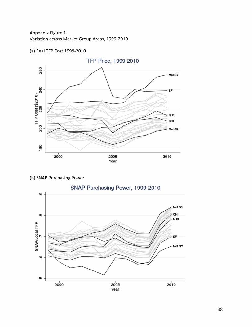
second half of 2009 and throughout 2010. Appendix Figure 1a shows the trends in the real TFP
cost for each of the market group areas. The figure demonstrates the general pattern of rising
TFP prices in 2005-2009 followed by a decline in 2010. Appendix Figure 1b shows SNAP
respectively) to compute a price for whole fruit in Hartford for the first quarter of 2002 (0.84×$0.218+0.16×$0.244 = $0.222 per 100 grams). 12 These results are available upon request.
9
purchasing power for the market group areas; this illustrates the variation in trends across
areas and shows clearly the effect of the ARRA.
2.2 National Health Interview Survey (NHIS) Data on SNAP Children
We use restricted-access micro data from the National Health Interview Survey (NHIS) for
the years from 1999-2010 to examine effects on child health and health care utilization.13 The
NHIS surveys approximately 35,000 households per year. By gaining restricted-use access to this
data we are able observe the county of residence for each household in the survey. This allows
us to link respondents to regional area food prices and access detailed information on
children’s health and the characteristics of their parents and households for a large and
representative national sample. From each household with children, the survey selects one
child at random (the “sample child”) and collects more extensive and detailed information on
this child’s health and health care utilization. Several of the outcomes we study are only
available in these Sample Child files, while others (e.g., parent-reported health status) are
available for all NHIS respondents in the Person-level file.
Our primary sample includes children ages 17 and under who are citizens of the United
States. We impose the citizenship restriction because the post-welfare reform era witnessed
dramatic changes to rules regarding non-citizens’ eligibility for many social safety net programs,
including SNAP.14 We conduct our main analyses on the sample of children in households who
13 State and county identifiers are masked in the public use NHIS data. Researchers interested in accessing the restricted
geocode data should contact Peter Meyer at [email protected]. 14 We test the robustness of our results to the inclusion of non-citizen children; these results are very similar to our main
results. See Appendix Tables 1 –2.
10
report having received SNAP benefits in at least one of the past 12 months. For the years from
1999 through 2010, there are 44,627 such children; 18,299 of them are also interviewed as
Sample Children. While the advantage of limiting our analysis to the SNAP recipients is clear
(this is the group most affected by SNAP), non-random selection into SNAP participation would
call into question a causal interpretation of our estimates. In Section 4.1, we analyze the
impact of SNAP purchasing power on SNAP participation at the county level and document no
significant relationship between the real value of SNAP benefits and the per-capita SNAP
caseload. As a robustness check in Section 5, we also test the sensitivity of our results using an
alternative sample with a high likelihood of being on SNAP—children living with low-educated,
unmarried parent(s).
Families with limited resources may respond to higher food prices by reducing consumption
of other goods that impact health, like ambulatory or preventive health care. Our primary
measures of health care utilization are indicators for whether the child has had a check-up in
the past 12 months and whether the child has had any doctor’s visit in the past 12 months.
According to guidelines from the American Academy of Pediatrics (AAP), children should have
6-7 preventive visits before age 1, 3 visits per year as 1-year olds, 2 visits as 2-year olds, and at
least one visit per year for ages 3 through 17. We also analyze the relationship between SNAP
purchasing power and whether (the parent reports that) a child has delayed or forgone care
due to cost in the past 12 months. Finally, we study whether the child has visited the ER in the
past year; if lower SNAP purchasing power reduces the use of preventive/ambulatory care, we
might expect higher area food prices to increase utilization of ER care.
We also analyze the effects of SNAP purchasing power on several direct measures of child
11
health that might respond to reduced nutrition, or to reduced consumption of other inputs in
the health production function (e.g., health care). Parental respondents report the child’s
health status on a 5-point scale (1—excellent, 2—very good, 3—good, 4—fair, and 5—poor); we
use this measure to construct an indicator for whether the child is in excellent or very good
health. As measures of contemporaneous health, we also study whether the child was
hospitalized over the past 12 months, the number of school days missed due to illness in the
past 12 months (for the sub-sample of school aged children), and an indicator for whether the
child missed 5 or more days of school due to illness. In addition, we estimate the relationship
between SNAP purchasing power and two longer-term health outcomes that may respond to
reduced nutrition or to food insecurity: an indicator for obesity based on height and weight
data (for the subsample of children ages 12-17), and whether the child has emotional problems
(defined for the universe of children ages 4 and older).
Table 1 displays summary statistics for SNAP recipient children. As expected, SNAP children
are likely to be poor, live in single-parent households (only a third live with both parents), and
are disproportionately likely to be black or Hispanic. Because such a high fraction (72 percent)
of SNAP children receive Medicaid, the rate of uninsurance among this sample is low, at about
7 percent. Health care utilization and health outcomes are worse for SNAP children than for
the general population of citizen children in the U.S. Nearly one-quarter of SNAP children went
without a check-up in the past year, but 90 percent had at least some sort of doctor’s visit
during that time. ER utilization is high, at over 30 percent, and more than 5 percent report
having delayed or gone without care due to its cost. In terms of health, itself, SNAP children
have lower-than-average health status, miss more school days (5, on average, but one-third of
12
SNAP children missed 5 or more in the past year), and commonly have emotional problems (46
percent of SNAP children 4 or older).
2.3 State and County Control Variables
We include several variables to control for regional policies and prices that might affect
child health and be correlated with local food prices. First, we control for local labor market
conditions with the county unemployment rate. Second, we include a summary index of state-
level SNAP policies developed by Ganong and Liebman (2015), which incorporates measures for
simplified reporting, recertification lengths, interview format (e.g. in person or not), call
centers, online applications, Supplemental Security Income Combined Application Project,
vehicle exemptions for asset requirement and broad-based categorical eligibility. Third, we
control for other state policies including the minimum wage, state EITC, TANF maximum benefit
guarantee amounts, and Medicaid/State Children’s Health Insurance Program (CHIP) income
eligibility limits. Finally, and perhaps most importantly, we control for prices of other goods by
including HUD’s fair market rent (measured by county as the “40th percentile of gross rents for
typical, non-substandard rental units occupied by recent movers in a local housing market”15)
and regional Consumer Price Indices (CPIs) for non-food, non-housing categories (apparel,
commodities, education, medical, recreation, services, transportation and other goods and
services). These are available for 26 metro areas; for the remaining areas, the CPI is calculated
within each of the four census regions and for four county population sizes (<50,000, 50,000-
1.5 million, >1.5 million).
15 More specifically, HUD estimates FMRs for 530 metropolitan areas and 2,045 nonmetropolitan county FMR areas.
13
2.4 Supplemental Data on SNAP Caseloads and Food Insecurity
We investigate the relationship between SNAP purchasing power and SNAP participation in
Section 4.1, using administrative data on county-level SNAP caseloads from the U.S.
Department of Agriculture (USDA), for the years from 1999 through 2010. We match each
county-year observation to that year’s TFP price for the market group to which the county
belongs.
To further probe mechanisms whereby variation in regional food prices may impact child
health, we supplement our main analysis by studying the relationship between SNAP
purchasing power and food insecurity. 16 For this analysis we use data from the December
Current Population Survey Food Security Supplement (CPS-FSS) for the years from 2001-2010.17
We identify a sample of 37,277 citizen children, ages 0 to 17, who live in households that report
receiving SNAP, and link them to market area TFP prices according to location of residence.18
3. Empirical Methods
We estimate the causal impact of variation in the real value of SNAP benefits on measures
16 Food insecurity is a household-level measure of well-being, defined as being unable to obtain, or uncertain of obtaining, an
adequate quantity and quality of food due to money or resources. Very-low food insecurity is defined as food insecurity that includes disrupted or restricted dietary patterns. Prior to 2006, very-low food insecurity was labeled “food insecurity with hunger”. 17 The December food security supplement was not collected in 1999 and 2000. 18 The public-use food security supplement files reports geographic information on all states, 217 counties, 69 primary
metropolitan statistical areas, 173 metropolitan statistical areas (MSA), 40 combined statistical areas (CSA), and 278 core-based statistical areas (CBSA) during our period of analysis. In order to assign CPS observations to a market group, we first identify states that include a single market group and assign all observations in that state to the corresponding market group. Continuing with the next most general geography (CSA), we repeat this process at increasingly more detailed geographies levels to the county identifiers. After this step, we then assign observations living in a non-metropolitan area to the rural market group based on their state of residence (for states with rural areas in a single market group). We match 83.7 percent of CPS observations to a market group using this iterative process.
14
of child health and health care utilization for children in households who report receiving SNAP
benefits during the past 12 months. Throughout, our regressions take the following form:
(1) 𝑦𝑖𝑟𝑡 = 𝛼 + 𝛽 ln (𝑆𝑁𝐴𝑃𝑀𝐴𝑋𝑡
𝑇𝐹𝑃𝑟𝑡) + 𝑋𝑖𝑟𝑡𝜃 + 𝑍𝑟𝑡𝛾 + 𝛿𝑡 + 𝜆𝑟 + 휀𝑖𝑟𝑡
where 𝑦𝑖𝑟𝑡 is the health outcome of individual i who resides in region r in time t. The key
independent variable is the natural log of the ratio of maximum SNAP benefits for a family of
four (which vary by year, but is constant across regions) to the regional TFP price. The vector Xirt
contains a set of controls for the child’s characteristics, including his/her age (and its square),
race, Hispanic ethnicity, family size, indicators for the presence of the mother (and/or father) in
the household, and interactions between indicators for the mother's (father's) presence and
the mother's (father's) education, marital status, age, and citizenship. The state policy variables
described in Section 2.3 are included in Zrt, as are a set of regional CPIs in non-food, non-
housing consumption categories. All models also include a full set of fixed effects for the year
(δt) and market group (r). The standard errors are clustered at the market group level.
We have also tested models with additional controls including income, parent-reported
health status, and an indicator for insurance coverage, but due to endogeneity concerns, we do
not include these in our main specification. The results are generally similar, however, and we
report these estimates in the supplementary appendix (Appendix Tables 3 and 4).
Identification in this model comes from variation in trends in the price of the Thrifty Food
Plan across market areas. As we showed earlier in Figure 1, there is substantial variation across
geographic areas in the purchasing power of SNAP benefits. In lower cost areas the SNAP
benefit covers up to 80 percent of the cost of the TFP, while in higher cost areas this falls to less
15
than 65 percent.19 More importantly for our identification strategy, these regional differences
change over time, with some areas experiencing larger increases in SNAP purchasing power
from 1999 to 2010, and others experiencing smaller increases (e.g., purchasing power in some
southern metropolitan areas increased nearly 17 percent, but only about 4.5 percent in urban
New York).20
4. Results
4.1 SNAP Participation
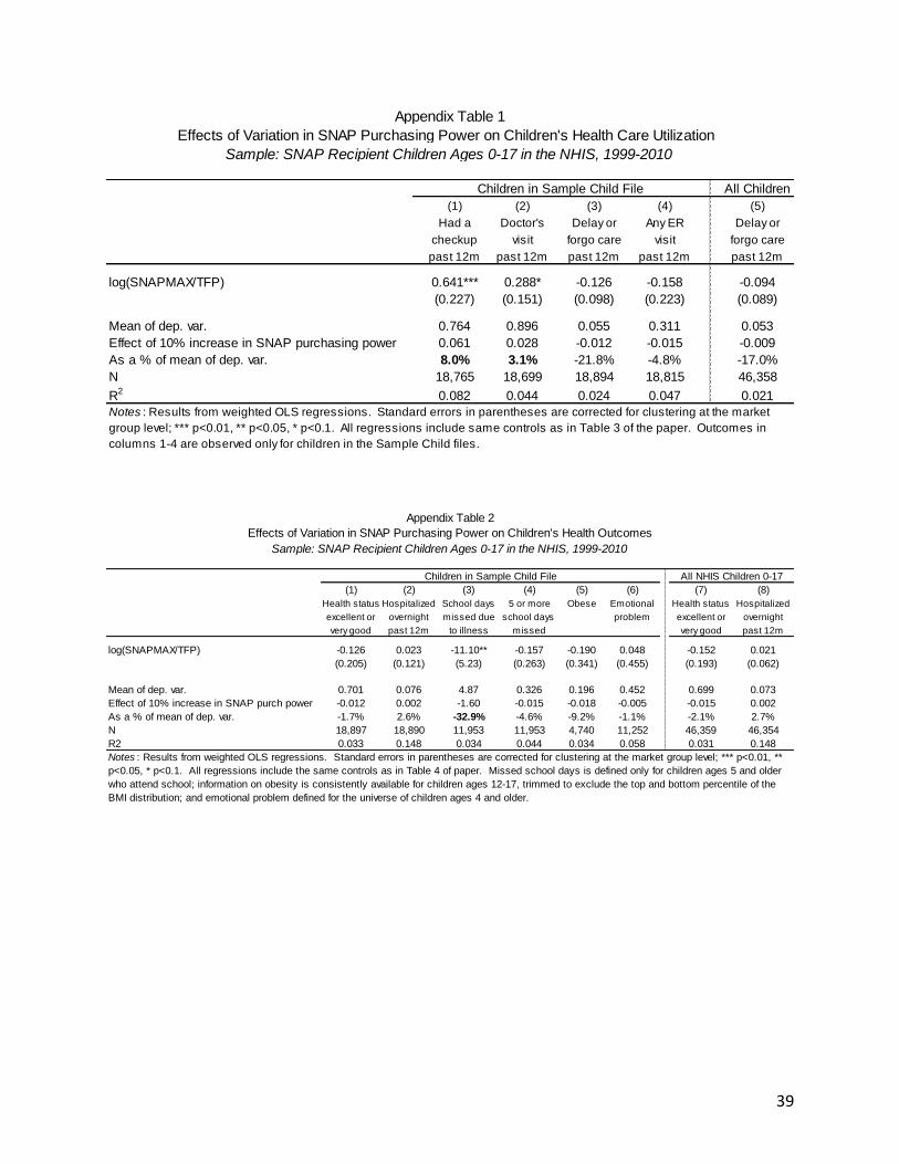
We begin by analyzing the effects of SNAP purchasing power on the SNAP caseload. If
variation in the real value of SNAP leads to changes in SNAP participation, then selection may
bias our estimates of the effect of SNAP purchasing power on child health.
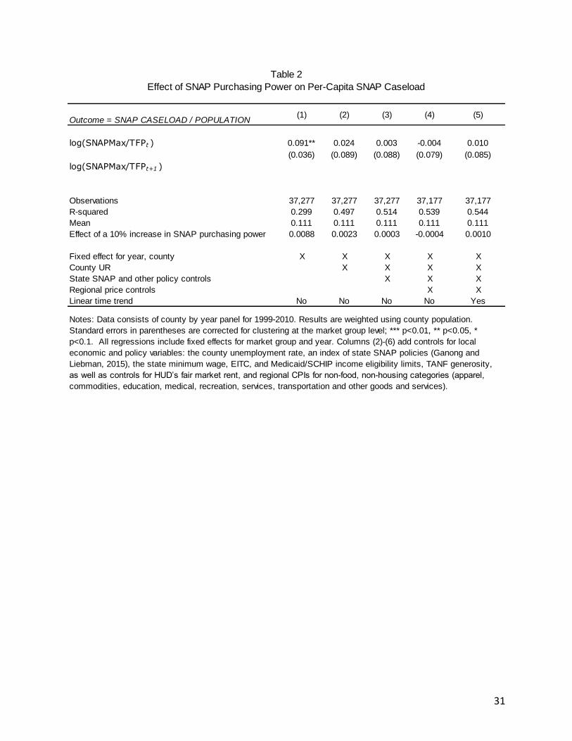
Using data from USDA, we construct a county panel for annual SNAP caseloads covering
1999-2010. We estimate equation (1) where the dependent variable is SNAP caseloads divided
by county population. Table 2 displays the results of six different specifications of the model.
Each includes year and market group fixed effects, as well as the (log) of the ratio of maximum
SNAP benefits to the market group TFP price. In the second column we add a control for the
county unemployment rate, which is a significant determinant of SNAP caseloads (Bitler and
Hoynes 2016) and possibly correlated with regional prices. In column 3 we add controls for
19 Note that since the statutory TFP is constructed using a national average, some areas are, by definition, likely to have SNAP
benefits that more than cover the cost of the TFP. However, our construction of market group TFP is unlikely to be exactly identical to the statutory definition. For our identification strategy to be valid however, all that matters is the relative generosity across market groups and trends across market groups. 20 SNAP benefits in 2010 and 6 months of 2009 include increased benefits provided through the American Recovery and
Reinvestment Act (ARRA). ARRA benefits amounted to $62, or about a 13.6 percent increase above the base 2009 levels. Changes in SNAP purchasing power ranged from a decrease of 5.8 percent in San Francisco to 4.3 percent increase in metropolitan areas in Arkansas and Oklahoma over the 1999-2008 period.
16
state policy variables, including for SNAP, EITC, minimum wages, TANF generosity, and
Medicaid. In column 4 we add controls for regional prices, including the county HUD fair market
rent and regional CPIs for goods other than food.
When only year and market group fixed effects are included, the estimated coefficient on
SNAP purchasing power is positive and significant, consistent with the SNAP caseload per capita
rising when the TFP decreases (and the real value of SNAP increases). However, once any
additional controls are added (e.g., even just the county unemployment rate, in column 2), the
coefficient drops substantially in magnitude and is no longer statistically different from zero.
The addition of the state policy controls (column 3) and the regional prices (column 4) result in
an estimate that is even smaller in magnitude. In columns 5, we extend the specification by
including a market group linear time trend which leads to little change in the estimated
coefficient on SNAP purchasing power. From this we conclude that there is no significant
relationship between the real value of SNAP and SNAP caseloads, and thus we interpret our
main results free of concerns about selection.
4.2 SNAP Purchasing Power and Health Care Utilization
The primary goal of our study is to analyze the impacts of variation in the purchasing power
of SNAP benefits on outcomes related to child health. We begin by examining evidence for
measures of health care utilization, recognizing that families facing higher food prices may
respond to the lower real value of their SNAP benefits by reducing out-of-pocket spending on
other goods, including health care.
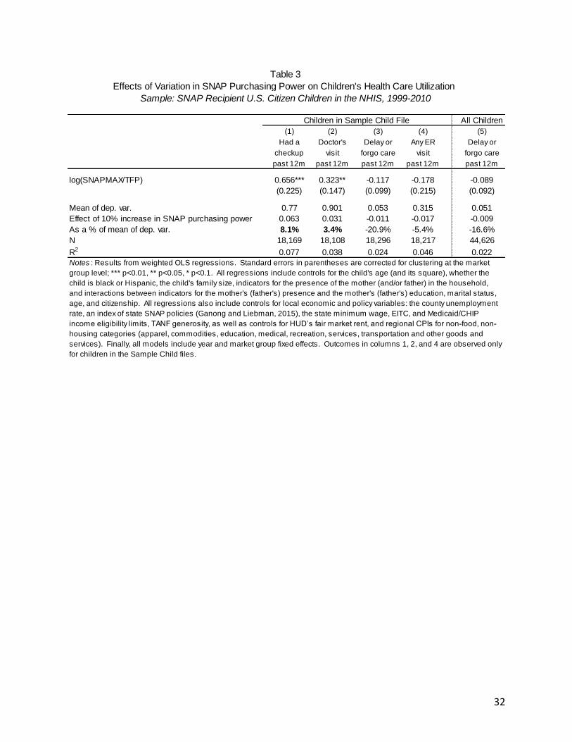
We present the results of this analysis in Table 3. Our primary measure of health care
17
utilization is an indicator for whether the child has had a check-up in the past 12 months
(column 1), which is observed only for children in the Sample Child file. We also examine
indicators for whether the child has had any doctor’s visit in the past 12 months (column 2),
whether the child has delayed or gone without care in the past 12 months due to cost (column
3), and whether a child has visited an ER in the past 12 months (column 4). Whether a child has
delayed or forgone care is reported in the Person file of the NHIS so is observed for all NHIS
children under age 18; we report this estimate in column 5. The model includes fixed effects for
market group, year, individual controls, and regional controls for unemployment rate, non-food
prices, and state safety net policies (similar to column 4 of Table 2).21 The key independent
variable, representing the real value of SNAP, is ln(SNAPMAX/TFP).
Among SNAP-recipient children, we find that increased purchasing power of SNAP
significantly raises the likelihood a child has had a checkup in the past 12 months. A ten
percent increase in the ratio (SNAPMAX/TFP) leads to a 6.3 percentage point (or 8.1 percent)
increase in the likelihood of a checkup. We also document a smaller, but significant impact of
increased SNAP purchasing power on the probability a child has had any doctor’s visit over the
past 12 months. A ten percent increase in the purchasing power of SNAP lowers the likelihood
of delaying/forgoing care by 3.1 percentage points, or 3.4 percent.
The results in columns 3 through 5 indicate that SNAP purchasing power has no statistically
significant effect on whether children are reported to have delayed or forgone care due to cost
(among all children or in the Sample Child sample), or on whether they have visited the ER in
21 Individual-level controls include the child's age (and its square), whether the child is black or Hispanic, the child's family size,
indicators for the presence of the mother (and/or father) in the household, and interactions between indicators for the mother's (father's) presence and the mother's (father's) education, marital status, age, and citizenship.
18
the past 12 months. However, the coefficients are all negative, suggesting a protective effect of
SNAP.
Broadly, we interpret these results as suggesting that children in households facing higher
food prices (and thus, lower SNAP purchasing power) receive less preventive and ambulatory
care.
4.3 SNAP Purchasing Power and Health Outcomes
Table 4 presents evidence on the extent to which variation in SNAP purchasing power
affects child health outcomes. The regression specifications include the same set of controls as
in Table 3. Note that several of the outcomes are defined only for sub-samples of children,
leading to different numbers of observations across the columns of Table 4. Specifically,
obesity is measured only for children ages 12 through 17,22 emotional problems are identified
for children ages 4 and older, and the number of school days missed is recorded only for
children age 5 and older who are in school. Parent-reported health status and hospitalization in
the past 12 months are reported for all children, but the other health outcomes are only
provided for children in the Sample Child file.
We find no statistically significant relationship between SNAP purchasing power and an
indicator for the child’s (parent-reported) health status being excellent or very good, nor the
likelihood of having been hospitalized in the past year. However, we document a strong
22 The indicator for obesity is based on BMI calculations, which are affected by some outlying height and weight
measurements. We trim the top and bottom of the BMI distribution to exclude the top and bottom percentile. In addition, height and weight information was only collected for children ages 12 and older in years 2008 through 2010. We therefore limit the sample to children ages 12-17.
19
negative and robust relationship between the real value of SNAP and the number of school
days children missed due to illness. For SNAP recipient children, a ten percent increase in SNAP
purchasing power is associated with a decrease in missed school days of just over 1 day (or a 22
percent decrease relative to the mean of approximately 5 days missed).
We find no statistically significant effects of real SNAP benefits on obesity nor the
propensity to have emotional problems, although we note that these are longer term health
problems that often develop over time and may be less likely to respond contemporaneously to
higher area food prices. It is possible that these outcomes would be likely to respond only after
a longer, cumulative period of food insecurity, poor nutrition, or reduced health care.
We interpret these results as suggesting that variation in the real value of SNAP may have
some modest impacts on children’s contemporaneous health. A weakness of measuring health
using the number of school days missed due to illness is that it may depend on the parent’s
evaluation of the child’s health; however, parent-reported health status, which is also a
subjective measure, does not appear to respond to variation in the real value of SNAP. On the
other hand, the number of missed school days is perhaps the only health outcome we analyze
that might be expected to respond contemporaneously to reduced nutrition or limited use of
preventive/ambulatory health care.
5. Mechanisms and Robustness Checks
5.1 SNAP Purchasing Power and Food Insecurity
One avenue through which higher area food prices may impact child health is by reducing
households’ consumption of preventive and ambulatory health care for their children. The
20
results in Section 4, which point to a significant reduction in yearly check-ups and doctor’s visits
for those with lower SNAP purchasing power, are consistent with such a mechanism.
However, variation in SNAP purchasing power may also affect health more directly, if
children facing higher area food prices are able to consume less (or less nutritious) food.
Because the NHIS did not provide information on food security or nutritional intake in the years
of data we analyze, we turn to data from the December food security supplement to the CPS to
estimate the impact of SNAP purchasing power on food insecurity among SNAP-recipient
children.
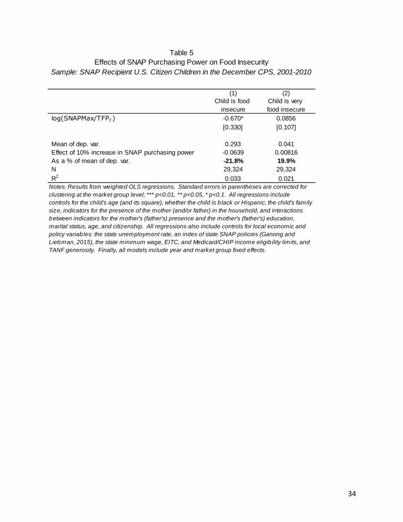
We display these results in Table 5. The regression specifications include the same set of
controls as in Tables 3 and 4. We find that a higher real value of SNAP benefits is associated
with an improvement in children’s food security: A 10 percent increase in SNAP purchasing
power reduces the likelihood a child is food insecure by 6.7 percentage points (a 21.8 percent
decrease relative to the mean). The result for very low food security is not statistically
significant; however, we note that very low food security is a fairly rare outcome even for SNAP
children (only 4 percent of the children in our sample are very food insecure while almost 30
percent are food insecure). In particular, very low food security requires not only that
households are uncertain of obtaining an adequate quantity and quality of food due to money
or resources, but that they also restrict or disrupt food intake because of lack of resources. It is
perhaps not surprising, then, that this more extreme outcome is not significantly responsive to
marginal variation in area food prices.
5.2 SNAP Purchasing Power and Health Insurance Coverage
21
In Table 6 we investigate whether the documented impacts of SNAP purchasing power on
health care utilization and health could be explained by a relationship between regional food
prices and health insurance coverage. Such a relationship would be unexpected for this
sample, given that SNAP recipient children are all likely to be income-eligible for Medicaid or
CHIP. Returning to our sample of NHIS children, we estimate equation (1), where the
dependent variable is now an indicator for whether the child is uninsured. Reassuringly, for
both children in the Sample Child file and all NHIS children, we find no statistically significant
effect of SNAP purchasing power on the likelihood a child has no health insurance.
5.3 Robustness Checks
A natural check of our main results is to estimate our models for health care utilization and
health outcomes on a “placebo” sample of children that should not be directly affected by
SNAP purchasing power (i.e., who are not impacted by SNAP benefits and whose health and
health care should not be as vulnerable to higher area food prices).
In Table 7 we present regression results analogous to those in Tables 3 and 4, but for a
sample of NHIS children living in households with incomes between 300 and 450 percent of the
federal poverty line.23 Estimated coefficients for our key outcomes (i.e., had check-up, had any
doctor’s visit, and number of school days missed) are small and statistically insignificant. This is
true for most other outcomes, as well. Two exceptions are that we find a statistically significant
effect of SNAP purchasing power on whether a child in this placebo sample visited the ER in the
23 As before, this sample is limited to children ages 0 through 17 who are citizens of the United States.
22
past year and on whether a child is obese. Recall that neither of these outcomes was found to
respond significantly to SNAP purchasing power among SNAP recipient children.
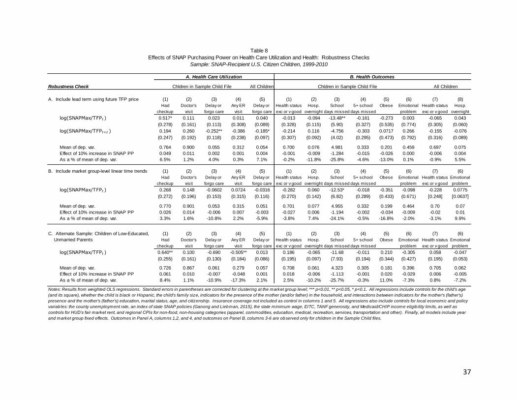
Table 8 displays the results of a series of robustness checks to our main findings regarding
the impacts of SNAP purchasing power on health care utilization and health. In panel A, we re-
estimate the models including a lead term that uses the t+1 market area TFP price. This lead
specification provides a test for the validity of our fixed effects design. If we find significant
effects of future prices (while controlling for current prices) we might be concerned that we are
capturing the effects of some other trend in the regions. That is, we estimate:
(2) 𝑦𝑖𝑟𝑡 = 𝛼 + 𝛽1 ln (𝑀𝐴𝑋𝑆𝑁𝐴𝑃𝑡
𝑇𝐹𝑃𝑟𝑡) + 𝛽2 ln (
𝑀𝐴𝑋𝑆𝑁𝐴𝑃𝑡+1
𝑇𝐹𝑃𝑟,𝑡+1)𝑋𝑖𝑟𝑡𝜃 + 𝑍𝑟𝑡𝛾 + 𝛿𝑡 + 𝜆𝑟 + 휀𝑖𝑟𝑡
In 11 of the 13 specifications, the lead of SNAP purchasing power is insignificant.
Additionally, our results for the contemporaneous effect of SNAP purchasing power are largely
unchanged: The magnitudes of the estimated coefficients for “had checkup” and “school days
missed” are quite similar to those in Tables 3 and 4. One exception is that the estimated impact
of current-period SNAP purchasing power on whether a child had any doctor’s visit in the past
12 months is a third as large and is no longer statistically significant.
The second panel of Table 8 contains results from a model that includes a set of market
group linear time trends. This approach places serious demands on the data in that
identification now must come from departures in market groups’ TFP prices from their trends
(assumed to be linear). While the main estimates for health care utilization (had checkup, had
any doctor’s visit) are qualitatively similar to those in Table 3, they are smaller in magnitude
and no longer statistically significant. The estimated impact of SNAP purchasing power on
missed school days, however, remains nearly identical in magnitude and significance to that in
23
Table 4.
Finally, to address concerns that inclusion in our SNAP recipient sample may be endogenous
to SNAP purchasing power, we estimate the impacts of variation in SNAP purchasing power on
health care utilization and health for a high intent-to-treat population. In particular, we identify
a sample of children living with unmarried parent(s) with less than a college education.24 Again,
the estimated impacts on the likelihood of a checkup and on the number of missed school days
are quite similar in magnitude to those for our main sample (although the p-value on the
coefficient for missed school days rises to 0.141). The estimated relationship between SNAP
purchasing power and having had any doctor’s visit is smaller and no longer statistically
significant. Interestingly, we document a negative effect of increased SNAP purchasing power
on ER utilization for this somewhat higher-income sample: a 10 percent increase in the ratio
(SNAPMAX/TFP) reduces the likelihood of an ER visit by 4.8 percentage points.
6. Discussion and Conclusion
In this paper we provide the first direct evidence on how variation in the real value of SNAP
benefits affects children’s health care utilization and health outcomes. We find evidence
consistent with families adjusting to higher area food prices (and thus, lower SNAP purchasing
power) by reducing utilization of preventive/ambulatory medical care. In particular, we
document that a 10 percent increase in SNAP purchasing power increases the likelihood a child
had a check-up in the past year by 8.1 percent and increases the likelihood that children had
24 Even though this is a high-ITT group, observable characteristics show that it is more advantaged, on average, than the SNAP
population.
24
any doctor’s visit in the past 12 months by 3.4 percent.
We do not find much evidence that these higher prices cause detrimental impacts on health
status, the likelihood of a hospitalization, or other measures of physical (e.g., obesity) and
mental health (e.g., child has emotional problems). One exception is that children facing higher
food prices (and thus, lower SNAP purchasing power) miss significantly more days of school due
to illness (22 percent more, relative to a baseline mean of 5 missed days, when SNAP
purchasing power is reduced by 10 percent). We also find that lower purchasing power of
SNAP benefits results in a greater likelihood of food insecurity.
One possible explanation for our finding stronger effects on utilization than on health itself
is that most of the health measures we consider are more chronic and cumulative in nature
(e.g., obesity). However, we also find no evidence of a relationship between SNAP purchasing
power and caregiver-reported health status, an outcome which could be less likely to suffer
from the same problem. A second possible interpretation of our findings is that while lower
SNAP purchasing power causes reduced health care utilization among children and negatively
affects food security, neither translates into substantial detrimental impacts on children’s
health status.
We also note that our measure of variation in the price of food is constructed using 30
market regions that perhaps mask variation in urban and rural customers who are in fact paying
different prices, thus masking why certain SNAP recipients are able to buy relatively
inexpensive food and stay relatively healthy. In related work, Bronchetti, Christensen, and
Hansen (2017) use food prices measured at a much finer level from the Food Acquisition and
Purchase Survey (FoodAPS) and demonstrate that the size of the geographic radius used to
25
measure whether SNAP benefits were sufficient to buy the TFP (at a store inside the radius)
mattered relatively little. What mattered far more is whether recipients were able to identify
and travel to a low cost store in the area. Still, we are optimistic that using datasets with finer
geographic variation in food prices may be a fruitful research area in the future.
Finally, our results speak to whether adjusting benefit levels to account for geographic
variation in food prices across market regions (30 nationally) would help improve child health
and wellbeing. We conclude that such adjustment would reduce disparities in child healthcare
utilization and school absenteeism in low-income households, but may not lead to significant
improvements in contemporaneous health status.
26
References
Almond, Douglas, Hilary W. Hoynes, and Diane Whitmore Schanzenbach. 2011. “Inside the War on Poverty: The Impact of Food Stamps on Birth Outcomes.” Review of Economics and Statistics 93 (2): 387–403. doi:10.1162/REST_a_00089.
Bitler, Marianne, and Hilary Hoynes. 2016. “The More Things Change, the More They Stay the Same? The Safety Net and Poverty in the Great Recession.” Journal of Labor Economics 34 (S1): S403–44. doi:10.1086/683096.
Breen, Amanda B., Rachel Cahill, Stephanie Ettinger de Cuba, John Cook, and Mariana Chilton. 2011. “Real Cost of a Healthy Diet: 2011.” Children’s Health Watch. http://www.childrenshealthwatch.org/publication/real-cost-of-a-healthy-diet-2011/.
Carlson, Andrea, Mark Lino, Wen Yen Juan, Kenneth Hanson, and P. Peter Basiotis. 2007. “Thrifty Food Plan, 2006.” CNPP-19. US Department of Agriculture, Center for Nutrition Policy and Promotion. http://www.cnpp.usda.gov/sites/default/files/usda_food_plans_cost_of_food/TFP2006Report.pdf.
Coleman-Jensen, Alisha, Mark Nord, Margaret Andrews, and Steven Carlson. 2014. “Household Food Security in the United States in 2011.” United States Department of Agriculture, Economic Research Service. Accessed February 19. http://www.ers.usda.gov/publications/err-economic-research-report/err141.aspx#.UwUzBV5kK-0.
Currie, Janet, and Enrico Moretti. 2008. “Short and Long-Run Effects of the Introduction of Food Stamps on Birth Outcomes in California.” In Making Americans Healthier: Social and Economic Policy as Health Policy. New York: Russel Sage.
East, Chloe N. 2016. “The Effect of Food Stamps on Children’s Health: Evidence from Immigrants’ Changing Eligibility.” University of Colorado Denver. http://cneast.weebly.com/uploads/8/9/9/7/8997263/east_jmp.pdf.
Ganong, Peter, and Jeffrey Liebman. 2015. “The Decline, Rebound, and Further Rise in SNAP Enrollment: Disentangling Business Cycle Fluctuations and Policy Changes.” Harvard University. http://scholar.harvard.edu/files/ganong/files/draftapr07manuscript.pdf.
Gregory, Christian A., and Alisha Coleman-Jensen. 2013. “Do High Food Prices Increase Food Insecurity in the United States?” Applied Economic Perspectives and Policy 35 (4): 679–707. doi:10.1093/aepp/ppt024.
Gregory, Christian A., and Partha Deb. 2015. “Does SNAP Improve Your Health?” Food Policy 50 (January): 11–19. doi:10.1016/j.foodpol.2014.09.010.
Gregory, Christian A., Michele Ver Ploeg, Margaret Andrews, and Alisha Coleman-Jensen. 2013. “Supplemental Nutrition Assistance Program (SNAP) Participation Leads to Modest Changes in Diet Quality.” 147. Economic Research Report. USDA Economic Research Service. https://www.ers.usda.gov/webdocs/publications/err147/36939_err147.pdf.
Gundersen, Craig, Brent Kreider, and John Pepper. 2011. “The Economics of Food Insecurity in the United States.” Applied Economic Perspectives and Policy 33 (3): 281–303.
Hoynes, Hilary, and Diane Whitmore Schanzenbach. 2016. “US Food and Nutrition Programs.” In Economics of Means-Tested Transfer Programs in the United States, Volume I.
27
University Of Chicago Press. http://www.press.uchicago.edu/ucp/books/book/chicago/E/bo23520704.html.
Hoynes, Hilary, Diane Whitmore Schanzenbach, and Douglas Almond. 2016. “Long-Run Impacts of Childhood Access to the Safety Net.” American Economic Review 106 (4): 903–34. doi:10.1257/aer.20130375.
Mykerezi, Elton, and Bradford Mills. 2010. “The Impact of Food Stamp Program Participation on Household Food Insecurity.” American Journal of Agricultural Economics 92 (5): 1379–1391.
Nord, M., and M. Golla. 2009. “Does SNAP Decrease Food Insecurity? Untangling the Self-Selection Effect. USDA.” United States Department of Agriculture, Economic Research Service.
Ratcliffe, Caroline, Signe-Mary McKernan, and Sisi Zhang. 2011. “How Much Does the Supplemental Nutrition Assistance Program Reduce Food Insecurity?” American Journal of Agricultural Economics 93 (4): 1082–98. doi:10.1093/ajae/aar026.
Renwick, Trudi, and Liana Fox. 2016. “The Research Supplemental Poverty Measure: 2011 - P60-258.Pdf.” Current Population Reports. US Census Bureau. https://www.census.gov/content/dam/Census/library/publications/2016/demo/p60-258.pdf.
Schmeiser, Maximilian D. 2012. “The Impact of Long-Term Participation in the Supplemental Nutrition Assistance Program on Child Obesity.” Health Economics 21 (4): 386–404. doi:10.1002/hec.1714.
Schmidt, Lucie, Lara Shore-Sheppard, and Tara Watson. 2016. “The Effect of Safety-Net Programs on Food Insecurity.” Journal of Human Resources 51 (3): 589–614. doi:10.3368/jhr.51.3.1013-5987R1.
Shaefer, H Luke, and Italo Gutierrez. 2011. “The Effects of Participation in the Supplemental Nutrition Assistance Program on the Material Hardship of Low-Income Families with Children.” Ann Arbor, MI: National Poverty Center, Gerald R. Ford School of Public Policy, University of Michigan.
“Supplemental Nutrition Assistance Program: Examining the Evidence to Define Benefit Adequacy.” 2013. Institute of Medicine and National Research Council. http://www.iom.edu/Reports/2013/Supplemental-Nutrition-Assistance-Program-Examining-the-Evidence-to-Define-Benefit-Adequacy.aspx.
Todd, Jessica E., Ephraim Leibtag, and Corttney Penberthy. 2011. “Geographic Differences in the Relative Price of Healthy Foods.” United States Department of Agriculture, Economic Research Service. http://books.google.com/books?hl=en&lr=&id=4qm5sgn3u20C&oi=fnd&pg=PP5&dq=todd+qfahpd&ots=UPHWMF7gnM&sig=6wOvjI4JceZtjJ-d7S111pPJm2w.
Todd, Jessica E., Lisa Mancino, Ephraim S. Leibtag, and Christina Tripodo. 2010. “Methodology behind the Quarterly Food-at-Home Price Database.” United States Department of Agriculture, Economic Research Service. http://ideas.repec.org/p/ags/uerstb/97799.html.
Yen, Steven T. 2010. “The Effects of SNAP and WIC Programs on Nutrient Intakes of Children.” Food Policy 35 (6): 576–83. doi:10.1016/j.foodpol.2010.05.010.
28
Yen, Steven T., Margaret Andrews, Zhuo Chen, and David B. Eastwood. 2008. “Food Stamp Program Participation and Food Insecurity: An Instrumental Variables Approach.” American Journal of Agricultural Economics 90 (1): 117–132.
Ziliak, James. 2015. “Temporary Assistance for Needy Families.” In SNAP Matters: How Food Stamps Affect Health and Well-Being. Stanford University Press.
Ziliak, James P. 2015. “Why Are So Many Americans on Food Stamps?” In SNAP Matters: How Food Stamps Affect Health and Well-Being, 18-. Stanford University Press.
29
Figure 1: Purchasing Power of SNAP by Market Group Panel A: 1999
Panel B: 2008
Panel C: 2010
Notes: Maps plot SNAPMAX/TFP for each of the 30 market areas identified consistently in the Quarterly Food at Home Price Database (QFAHPD).
30
Notes:
Sample All Sample All
Children Children Children Children
TFP price 203 203 Any check-up (12m) 0.770 --
(14) (14) (0.421)
Max SNAP benefit 143 143 Any doctor's visit (12m) 0.901
(12) (12) (0.299)
Income to poverty ratio 0.965 0.896 Any ER visit (12m) 0.315
(0.803) (0.738) (0.465)
Child's age 7.4 7.5 Delay/forgo care (12m) 0.058 0.051
(5.2) (5.1) (0.234) (0.220)
Child is male 0.510 0.507
(0.500) (0.500)
Child is black 0.329 0.339 Health status exc. or v. good 0.712 0.700
(0.470) (0.473) (0.453) (0.458)
Child is Hispanic 0.240 0.260 Hospitalized overnight (12m) 0.086 0.075
(0.427) (0.439) (0.280) (0.263)
Mother is present 0.934 0.940 School days missed, illness (12m) 4.96 --
(0.248) (0.238) (9.36)
Father is present 0.373 0.393 5+ school days missed (12m) 0.332 --
(0.484) (0.488) (0.471)
Both parents 0.337 0.361 Obese 0.199 --
(0.473) (0.480) (0.399)
Child receives Medicaid 0.715 0.723 Emotional problem 0.464 --
(0.451) (0.448) (0.763)
Child has no health insurance 0.072 0.067
(0.258) (0.250)
Number of observations 18,299 44,627 18,299 44,627
Summary Statistics for Samples of U.S. Citizen Children in NHIS who Receive SNAP
Table 1
(Weighted sample means; standard deviations in parentheses)
Health Outcomes
Health Care UtilizationChild/Household Characteristics
Notes: Results from weighted OLS regressions. Standard errors in parentheses are corrected for clustering at the market group level; *** p<0.01, ** p<0.05, * p<0.1. All regressions include controls for the
child's age (and its square), whether the child is b lack or Hispanic, the child's family size, indicators for the presence of the mother (and/or father) in the household, and interactions between indicators for
the mother's (father's) presence and the mother's (father's) education, marital status, age, and citizenship. Insurance coverage not included as control in columns 1 and 5. All regressions also include
controls for local economic and policy variab les: the county unemployment rate, an index of state SNAP policies (Ganong and Liebman, 2015), the state minimum wage, EITC, TANF generosity and
Medicaid/CHIP income eligib ility limits, as well as controls for HUD’s fair market rent, and regional CPIs for non-food, non-housing categories (apparel, commodities, education, medical, recreation,
services, transportation and other goods and services). Finally, all models include year and market group fixed effects. Outcomes in Panel A, columns 1,2, and 4, and outcomes on Panel B, columns 3-6
are observed only for children in the Sample Child files.
Table 7
Effects of SNAP Purchasing Power on Health Care Utilization and Health: Robustness Checks
Sample: U.S. Citizen Children in NHIS with Household Incomes between 300 and 450 Percent of Federal Poverty Line, 1999-2010
A. Health Care Utilization B. Health Outcomes
Chldren in Sample Child File Chldren in Sample Child File All Children
Mean of dep. var. 0.726 0.867 0.061 0.279 0.057 0.708 0.061 4.323 0.305 0.181 0.396 0.705 0.062
Effect of 10% increase in SNAP PP 0.061 0.010 -0.007 -0.048 0.001 0.018 -0.006 -1.113 -0.001 0.020 -0.029 0.006 -0.005
As a % of mean of dep. var. 8.4% 1.1% -10.9% -17.3% 2.1% 2.5% -10.2% -25.7% -0.3% 11.0% -7.3% 0.8% -7.2%
Table 8
Effects of SNAP Purchasing Power on Health Care Utilization and Health: Robustness Checks
Sample: SNAP-Recipient U.S. Citizen Children, 1999-2010
A. Include lead term using future TFP price
Notes: Results from weighted OLS regressions. Standard errors in parentheses are corrected for clustering at the market group level; *** p<0.01, ** p<0.05, * p<0.1. All regressions include controls for the child's age
(and its square), whether the child is b lack or Hispanic, the child's family size, indicators for the presence of the mother (and/or father) in the household, and interactions between indicators for the mother's (father's)
presence and the mother's (father's) education, marital status, age, and citizenship. Insurance coverage not included as control in columns 1 and 5. All regressions also include controls for local economic and policy
variab les: the county unemployment rate, an index of state SNAP policies (Ganong and Liebman, 2015), the state minimum wage, EITC, TANF generosity, and Medicaid/CHIP income eligib ility limits, as well as
controls for HUD’s fair market rent, and regional CPIs for non-food, non-housing categories (apparel, commodities, education, medical, recreation, services, transportation and other). Finally, all models include year
and market group fixed effects. Outcomes in Panel A, columns 1,2, and 4, and outcomes on Panel B, columns 3-6 are observed only for children in the Sample Child files.
Chldren in Sample Child File All ChildrenChldren in Sample Child File
A. Health Care Utilization B. Health Outcomes
38
Appendix Figure 1 Variation across Market Group Areas, 1999-2010 (a) Real TFP Cost 1999-2010