University of Kentucky University of Kentucky

UKnowledge UKnowledge

Biosystems and Agricultural Engineering Faculty Publications Biosystems and Agricultural Engineering

5-2009

Local Head Loss of Non-Coaxial Emitters Inserted in Polyethylene Local Head Loss of Non-Coaxial Emitters Inserted in Polyethylene

Pipe Pipe

Osvaldo Rettore Neto University of São Paolo, Brazil

Jarbas Honorio de Miranda Universidade de São Paulo, Brazil

José Antonio Frizzone Universidade de São Paulo, Brazil

Stephen R. Workman University of Kentucky, steve.workman@uky.edu

Follow this and additional works at: https://uknowledge.uky.edu/bae_facpub

Part of the Agricultural Science Commons, and the Bioresource and Agricultural Engineering

Commons

Right click to open a feedback form in a new tab to let us know how this document benefits you. Right click to open a feedback form in a new tab to let us know how this document benefits you.

Repository Citation Repository Citation Neto, Osvaldo Rettore; de Miranda, Jarbas Honorio; Frizzone, José Antonio; and Workman, Stephen R., "Local Head Loss of Non-Coaxial Emitters Inserted in Polyethylene Pipe" (2009). Biosystems and Agricultural Engineering Faculty Publications. 205. https://uknowledge.uky.edu/bae_facpub/205

This Article is brought to you for free and open access by the Biosystems and Agricultural Engineering at UKnowledge. It has been accepted for inclusion in Biosystems and Agricultural Engineering Faculty Publications by an authorized administrator of UKnowledge. For more information, please contact UKnowledge@lsv.uky.edu.

Local Head Loss of Non-Coaxial Emitters Inserted in Polyethylene Pipe Local Head Loss of Non-Coaxial Emitters Inserted in Polyethylene Pipe

Digital Object Identifier (DOI) https://doi.org/10.13031/2013.27394

Notes/Citation Information Notes/Citation Information Published in Transactions of the ASABE, v. 52, issue 3, p. 729-738.

© 2009 American Society of Agricultural and Biological Engineers

The copyright holder has granted the permission for posting the article here.

This article is available at UKnowledge: https://uknowledge.uky.edu/bae_facpub/205

Transactions of the ASABE

Vol. 52(3): 729-738 � 2009 American Society of Agricultural and Biological Engineers ISSN 0001-2351 729

LOCAL HEAD LOSS OF NON‐COAXIAL EMITTERS

INSERTED IN POLYETHYLENE PIPE

O. Rettore Neto, J. H. de Miranda, J. A. Frizzone, S. R. Workman

ABSTRACT. The design of a lateral line for drip irrigation requires accurate evaluation of head losses in not only the pipe butin the emitters as well. A procedure was developed to determine localized head losses within the emitters by the formulationof a mathematical model that accounts for the obstruction caused by the insertion point. These localized losses can besignificant when compared with the total head losses within the system due to the large number of emitters typically installedalong the lateral line. An experiment was carried out by altering flow characteristics to create Reynolds numbers (R) from7,480 to 32,597 to provide turbulent flow and a maximum velocity of 2.0 m s‐1. The geometry of the emitter was determinedby an optical projector and sensor. An equation was formulated to facilitate the localized head loss calculation using thegeometric characteristics of the emitter (emitter length, obstruction ratio, and contraction coefficient). The mathematicalmodel was tested using laboratory measurements on four emitters. The local head loss was accurately estimated for theUniram (difference of +13.6%) and Drip Net (difference of +7.7%) emitters, while appreciable deviations were found for theTwin Plus (‐21.8%) and Tiran (+50%) emitters. The head loss estimated by the model was sensitive to the variations in theobstruction area of the emitter. However, the variations in the local head loss did not result in significant variations in themaximum length of the lateral lines. In general, for all the analyzed emitters, a 50% increase in the local head loss for theemitters resulted in less than an 8% reduction in the maximum lateral length.

Keywords. Contraction coefficient, Emitter, Head loss, Hydraulic radius.

rip irrigation pipes with integrated emitters alterthe velocity of water at the location of the emitterinsertion point, providing a significant localizedhead loss in addition to the head loss of the pipe,

as demonstrated by Juana et al. (2002a). To obtain highuniformity of water distribution in operational units, thehydraulic system design should consider the total head lossin the pipe and the small variations in head loss of the emittersalong the lateral line. However, the localized head losses aretypically neglected because few equations exist for easilycalculating these losses.

Since the head loss within the section of the emitterpassage does not depend on the viscous forces (Bagarello etal., 1997; Juana et al., 2002b), a model to calculate thelocalized head loss contains variables that define thegeometric relationships of the obstructing element and the

Submitted for review in January 2008 as manuscript number SW 7336;approved for publication by the Soil & Water Division of ASABE in April2009.

The authors are Osvaldo Rettore Neto, Agricultural Engineer,Graduate Student, Department of Agricultural Engineering, Luiz deQueiroz College of Agriculture, University of São Paulo, Piracicaba,Brazil; Jarbas Honorio Miranda, Associate Professor, Department ofExact Sciences, Luiz de Queiroz College of Agriculture, University of SãoPaulo, Piracicaba, Brazil; José Antonio Frizzone, Full Professor,Department of Agricultural Engineering, Luiz de Queiroz College ofAgriculture, University of São Paulo, Piracicaba, Brazil; and Stephen R.Workman, ASABE Member Engineer, Associate Professor, Departmentof Biosystems and Agricultural Engineering, University of Kentucky,Lexington, Kentucky. Corresponding author: Osvaldo Rettore Neto,Department of Agricultural Engineering, Luiz de Queiroz College ofAgriculture, University of São Paulo, Av. Pádua Dias, 11 CP 9 CEP13418‐900, Piracicaba, SP, Brazil; phone: +55‐19‐3429‐4217; fax:+55‐19‐3447‐8571; e‐mail: orettore@esalq.usp.br.

pipe. The main objective of this work was to formulate amathematical model to estimate the localized head lossstarting from an obstruction index of the emitter insertionpoint with applications of the conservation of energy andmass equations. Specifically, the obstruction affects thehydraulics of water inflow due to the abrupt reduction incross‐section of the pipe at the emitter and the subsequentreturn to full cross‐section after the emitter.

THEORYThe emitter insertion point along the lateral line modifies

the course of the water flow, causing local turbulence thatresults in localized head losses in addition to the lossesdistributed in the pipe. The turbulence is a consequence of thepresence of the insertion point along the internal wall of thepipe, which causes an obstruction in the inflow section, acontraction in the insert place, and a reduction in the inflowpipe diameter (Al‐Amoud, 1995; Bagarello et al., 1997;Juana et al., 2002a, 2002b; Provenzano and Pumo, 2004;Provenzano et al., 2005; Palau‐Salvador et al., 2006).

For mathematical simplicity, many designers of irrigationprojects prefer to use empirical equations like Hazen‐Williams, Manning, and Scobey to determine the head lossesinstead of using the theoretical equation of Darcy‐Weisbach.However, an important limitation of those empiricalequations is a roughness factor assumed constant for alldiameters and inflow speeds (Kamand, 1988). Due to thatsimplification, the head loss calculated by the empiricalequations can differ significantly from the calculations by theDarcy‐Weisbach equation in that the attrition factor varieswith the inflow conditions (Bombardelli and García, 2003).

D

730 TRANSACTIONS OF THE ASABE

The energy dissipation represented by the head loss inturbulent inflow of real fluids through cylindrical tubes canbe calculated by equations presented in the basic literature ofhydraulics (Porto, 1998). The most important contribution isexpressed by the equation of Darcy‐Weisbach (Kamand,1988; von Bernuth, 1990; Bagarello et al., 1995; Romeo etal., 2002; Sonnad and Goudar, 2006), whose form isexpressed by (eq. 1):

g

V

D

Lfhf

2

2

= (1)

where hf is head loss (m), L is pipe length (m), D is internaldiameter (m), V is mean water velocity at uniform pipesections (m s‐1), g is gravitational acceleration (m s‐2), and fis friction factor (dependent on the Reynolds number, R, andthe roughness of the pipe wall, ε).

The hydraulic resistance, expressed as the friction factor(f), constitutes the basic information to the hydraulic project.From the pioneering contributions made by Weisbach in1845, Darcy in 1857, Boussinesq in 1877, and Reynolds in1895 mentioned in the work by Yoo and Singh (2005), thehydraulic resistance to flow has been the object of continualinterest and study. Recently, the importance of head losses indrip irrigation has been recognized and has stimulated thedevelopment of mathematical equations to estimate them(Bagarello et al., 1997; Juana et al., 2002a, 2002b;Provenzano and Pumo, 2004; Provenzano et al., 2005; Palau‐Salvador et al., 2006).

Previous experimental research (von Bernuth and Wilson,1989; von Bernuth, 1990; Bagarello et al., 1995) showed thatin small‐diameter polyethylene pipes with Reynoldsnumbers (R) in the range 4,000 < R < 100,000, the frictionfactor can be expressed by an equation similar to the Blasiusequation (eq. 2):

2−= mRcf (2)

where c is a constant for the particular friction coefficientformula used, and m is the velocity (or flow rate) exponent.

Introducing c = 0.316 and m = 1.75 into the Blasiusequation provides an accurate estimation of the frictionallosses produced by turbulent flow inside uniform pipes withlow wall roughness and Reynolds numbers within the range4,000 < R < 100,000 (Juana et al., 2002a, 2002b; Yildirim,2006). According to the results of von Bernuth and Wilson(1989), c is a value in the range of 0.281 to 0.345. By usingpipe head loss per unit length measurements obtained from16, 20, and 25 mm nominal diameter pipes for R valuesranging from 3,000 to 36,000, Bagarello et al. (1995)proposed two simple criteria of f estimation based,respectively, on a purely empirical approach and asemitheoretical analysis. According to the empiricalapproach, the c coefficient of the Blasius equation assumesa constant value equal to 0.302.

The local head loss (hfe) in the emitters or around theirconnections with the lateral is due to the resistance caused bythe transport of water around the obstructing element insidethe pipe. This can be expressed in the classic form as afraction of the kinetic load (K), obtained by the Reynoldssimilarity principle (eq. 3):

g

VKhfe 2

2

= (3)

where hfe is local head loss (m), and K is coefficient of kineticload.

The coefficient K depends on the geometriccharacteristics of the emitter insertion point and the Reynoldsnumber (R). For a given pipe section (A), flow rate (Q), andfor a connection with defined dimensions, the value of K isreduced with an increase of R until a limit is reached fromwhich K remains approximately constant (Bagarello et al.,1997; Provenzano and Pumo, 2004). In practice, the effect ofthe viscous forces can be neglected for R > 10,000 accordingto Bagarello et al. (1997). In this case, the factor K can beexpressed by geometric relationships considering the inflowsection in the pipes and the obstructing element. For on‐lineemitters, the relationship between K and the geometry of theinflow section can be obtained using the theorem of Bélanger,applied to a sudden contraction of the section and subsequentenlargement, in that section (Ar = r·A), where r is theobstruction ratio, Ar represents the passage area for the fluidat the emitter insertion point, and A represents the passagearea for the pipe without the emitter.

By applying the theorems of energy and massconservation at a sudden enlargement among the sections Acand A, we have the equation of Bélanger (eq. 4):

( )g

V

A

A

g

VVhf

r

ce 2

12

222

⎟⎟⎠

⎞⎢⎢⎝

⎛−=−= (4)

Equation 4 shows that the local loss due to a suddenenlargement depends on the ratio IO = [(A ‐ Ar)/Ar]2, namedby Bagarello et al. (1997) as an obstruction index (eq. 5),which can be assumed representative of the obstruction dueto both the emitter protrusion and the pipe deformation:

221

1 ⎟⎠⎞⎢

⎝⎛ −=⎟⎟⎠

⎞⎢⎢⎝

⎛−=

r

r

A

AIO

r

(5)

where r is the obstruction ratio (r = Ar/A).Similarly, the presence of an on‐line emitter in a lateral

determines a local loss (hfe), due to the protrusion of emitterbarbs into the flow, that can be expressed as a K fraction ofthe kinetic height. Previous experimental investigationcarried out by Bagarello et al. (1997) showed that the Kcoefficient depends on the ratio between the pipe section (A)and the cross‐section area (Ac) where the emitter is located,according to the following relationship:

29.1

168.1 ⎟⎟⎠

⎞⎢⎢⎝

⎛−=

rA

AK (6)

obtained in the range 1.00 < A/Ar < 1.40.Although each individual emitter usually determines a

small local head loss given by equation 3, the sum of all suchlocal losses in a lateral line can become significant, sinceemitter spacing can be very small and many emitters areinserted along a lateral line. Results of Al‐Amoud (1995)indicate that there are significant energy losses due to theemitter connections. An increase in the energy loss of morethan 32% compared to plain pipe was observed for laterals of13 mm diameter.

The lateral lines of irrigation systems are made of flexiblepolyethylene of low density. Consequently, variations should

731Vol. 52(3): 729-738

1

2

3

4

67

5

Figure 1. Layout of the experimental installation for lateral drip testing: 1 = water tank, 2 = variable frequency controller, 3 = pump, 4 = screen filter,5 = drip lateral, 6 = differential manometer, and 7 = electromagnetic flowmeter.

be expected in the geometry along the pipe. These variationscan hinder the determination of the necessary measurementsrelative to the obstruction index due to the emitter protrusion.The r values can be modified by the effect of the operationpressure on the internal pipe diameter depending on thepolyethylene elasticity (Vilela et al., 2003). Therefore, the restimate should be made with a statistical base using medianvalues of Ar and A (Juana et al., 2002a).

MATERIALS AND METHODSThe research was carried out at the Irrigation Laboratory

of the Department of Agricultural Engineering, University ofSão Paulo, Piracicaba, Brazil. A testing bench for head losswas built for the control, monitoring, and acquisition of thenecessary data for the research development (fig. 1).

A variable frequency controller was connected to a pumpto maintain a constant rotation of the pump to avoid flowalterations caused by any voltage variation in the electricalfeed. It used water from the public network stored in areservoir inside the laboratory and operated in closed circuitsystem. An in‐line disk filter equivalent to 120‐mesh screenwas installed to remove particulates. Valves were connectedto control the flow in the line entrance. A digital pressuremonitor was used with range from 0 to 1,500 kPa and anaccuracy of ±1 kPa. During the tests, the pressure wasmaintained between 145 and 155 kPa to minimize thealteration of the pipe diameter, as described by Vilela et al.(2003).

The flow inside the pipe was measured by an inductivemagnetic flowmeter (±1% accuracy) installed at the end ofthe piping prior to the return to the reservoir. The head losswas measured by a differential manometer containing liquidwith density 1.5 (times water density).

DEVELOPMENT OF THE CONNECTION FOR MEASUREMENT OF HEAD LOSS

A pipe segment 1 m in length was used for the head lossdetermination. Commercial barb connections could not beused in the test procedure because they would introduceadditional head loss in the system, so a silicone hose (fig. 2)with a 10 mm external diameter and wall thickness of 2.5 mmwas fitted to the pipe. The hose was cut in several segmentsof 25 mm length. The hose was fastened with a fast‐dryingglue, with the purpose of adhering the silicone segment to thepipe, so that the pipe center was in the center of the siliconehose segment.

MEASUREMENT OF THE FRICTION HEAD LOSS A differential U‐type manometer was used to measure

head loss with a scale in mm (1,000 ‐ 0 ‐ 1,000). The

Figure 2. Silicone hose connection.

manometer was filled with a liquid having a density equal to1.5 (times water density). The head loss was measured in apipe segment 0.5 m in length. The manometer was connectedto the test system using the silicone connection describedabove.

The experimental tests were accomplished by measuring theflow through the pipe and the pressure difference between twopoints as registered by the U‐type manometer. The tests wereconducted for 19 to 21 flow rates for each pipe and repeated forten pipe samples. During the experiments, the watertemperature was measured every 30 min using a mercurythermometer with a 0.1°C scale. It varied from 20.5°C to24.5°C and was used to correct the kinematic viscosity of thewater in the determination of head loss. An optic profileprojector coupled to a microcomputer was used to determine theinternal diameter of the pipe. Table 1 shows the diameter andwall thickness of the pipes used in the experiment.

The experimental values of the head loss were used tocalculate f for equation 1, knowing the values of V2/2g, L, andD. To determine the value of the c coefficient (eq. 7), a linearregression was performed between the values of f and R‐0.25.

25.0−=R

cf (7)

Table 1. Characteristics of pipes used in the experiment.[a]

Average(mm)

SD(mm)

CV(%)

Internal diameter 15.53 0.134 0.86Wall thickness 1.07 0.06 5.61

[a] Ten samples were used to determine the characteristics.

732 TRANSACTIONS OF THE ASABE

Table 2. Characteristics of the emitters used in the experiment and the location of emitter within the pipe section.

Nominaldiameter (mm)

Internaldiameter (mm) Manufacturer Model

Flow(L h‐1)

EmitterSpacing (m)

ConnectionLength (m)

17.5 15.53 Irrimon Twin Plus 1.8 1.00 0.4817 14.23 Netafim Tiran 2.0 0.70 0.1717 14.09 Netafim Uniram 2.3 0.75 0.2017 14.98 Netafim Drip Net 1.6 0.75 0.20

To validate the methodology of using 0.5 m of pipesections to determine the friction head loss, the frictionfactor, f, in the pipe was compared with that calculated by themodel proposed by Bagarello et al. (1995). The experimentaltrials consisted of 193 measured pair points of flow head loss,in polyethylene pipe of 15.53 mm of internal diameter,resulting in Reynolds numbers ranging from 8,244 to 35,127.

DETERMINATION OF THE LOCAL HEAD LOSS DUE TO EMITTERS

Four types of emitters (Tiran, Uniram, Drip Net PC, andTwin Plus) were analyzed in the test apparatus andrepresented different geometric characteristics. Ten pipesamples were tested with each of the emitters. Due to thedifferent spacing among emitters, three different lengths ofpipe/emitter were used. These were 1.4 m for Tiran, 1.5 m forthe Uniram and Drip Net PC, and 2.0 m for Twin Plus. Afterthe initial tests, the emitters were sealed for subsequent testsso that the emitter obstruction could be evaluated. Table 2contains the characteristics of the emitter/pipe combinationsused in the experiment.

The head loss was determined between two points (1.0 mof pipe with emitter) for 15 flow values ranging from a lowof 0.342 m3 h‐1 to a maximum of 1.201 m3 h‐1. The maximumflow corresponded to a maximum velocity of 2 m s‐1. Thewater temperature was measured with a thermometer foreach test for subsequent use in the mathematical modeling.

For each discharge, the amount of local losses caused bythe emitter was calculated by the difference between the totalmeasured head losses of the 1.0 m segment with the sealedemitter and the corresponding friction losses evaluated byequations 1 and 2 for the section of pipe without an emitter,for c = 0.296. This procedure is in agreement with publishedresearch on local pressure losses for microirrigation laterals(Al‐Amoud, 1995; Bagarello et al., 1997; Provenzano andPumo, 2004).

DETERMINATION OF THE INFLOW SECTION

A key aspect of the experiment was the determination ofthe obstruction in the pipe created by the emitter. An opticalprojector (Starrett model HB 400) was used for thisdetermination. The equipment projects a light beam on theobject, which is enlarged by a magnifying glass. The image

is projected as a vertical image on a surface that contains theoptical sensor. The platform holding the object being studiedcan move in vertical and horizontal directions to allow theentire object to be detected by the sensor. The opticalprojector was coupled to a personal computer with softwaredeveloped by Metronics that interprets the signal sent by thesensor. With the integrated measurement system, it ispossible to determine a point, straight line, diameter,distance, angle, and semicircles.

The determination of the cross‐section of the emitterobstruction was accomplished in two stages. The first stagewas the geometric characterization of the emitter obstructionwith ten repetitions for each emitter/pipe combination. Thesecond stage was the determination of the characteristics ofthe pipe. Table 3 shows the geometric characteristics of theemitters studied with the optical projector. Table 4 illustratesthe shapes observed by the optical sensor for each of theemitters.

LOCAL HEAD LOSS MODEL

The head loss in pipes is inversely related to the pipediameter. Since the water flow section along the emitter is notcompletely circular, the mathematical model for head loss inthe emitter, hfe, was calculated based on the hydraulic radiususing the wetted perimeter (eq. 8):

m

rh P

AR = (8)

where Rh is hydraulic radius, Ar is passage area of the fluidfor the emitter, and Pm is wetted perimeter.

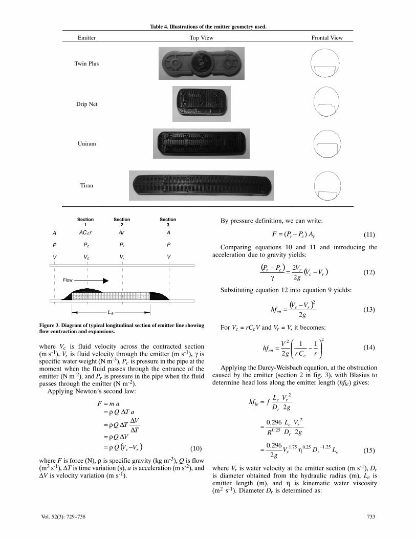
For the head loss determination in emitters, threecomponents are considered: head loss in the entrance (hfen),head loss in the emitter length (hfle), and head loss in the exit(hfex). Figure 3 shows the representation of an emitter inte-grated to the lateral line with the respective considerations forthe mathematical modeling.

Applying the Bernoulli theorem to sections 1 and 2permits head loss determination in the entrance (hfen):

⎟⎟⎠

⎞⎢⎢⎝

⎛�

−�

−−= crrcen

PP

g

V

g

Vhf

22

22

(9)

Table 3. Geometric characteristics and inflow for the different emitters.

Emitter

Geometric Characteristics and Inflow[a]

Observed Calculated

Amm2 (SD)

Aemm2 (SD)

Pmmm (SD)

Lemm (SD)

Armm2

Drmm

Ccmm

rmm

Twin plus 189 (3.27) 57.1 (0.561) 58.7 (0.241) 36.1 (0.111) 132 9.02 0.800 0.698Tiran 159 (2.23) 35.9 (0.516) 49.1 (0.142) 72.0 (0.042) 123 10.0 0.816 0.774

Uniram 156 (1.48) 69.9 (2.28) 51.8 (0.553) 44.6 (0.153) 86.0 6.65 0.775 0.552Drip net 176 (2.65) 53.7 (0.613) 52.8 (0.509) 21.5 (0.168) 122 9.28 0.796 0.695

[a] Variables are defined in the Nomenclature section.

733Vol. 52(3): 729-738

Table 4. Illustrations of the emitter geometry used.

Emitter Top View Frontal View

Twin Plus

Drip Net

Uniram

Tiran

A

P

V

AC r

P

V

Ar

P

V

A

P

V

Le

c

c

r

r

c

Section1

Section2

Section3

Flow

Figure 3. Diagram of typical longitudinal section of emitter line showingflow contraction and expansions.

where Vc is fluid velocity across the contracted section(m�s‐1), Vr is fluid velocity through the emitter (m s‐1), γ isspecific water weight (N m‐3), Pc is pressure in the pipe at themoment when the fluid passes through the entrance of theemitter (N m‐2), and Pr is pressure in the pipe when the fluidpasses through the emitter (N m‐2).

Applying Newton's second law:

( )rc VVQ

VQT

VTQ

aTQamF

−ρ=�ρ=

�

��ρ=

�ρ==

(10)

where F is force (N), ρ is specific gravity (kg m‐3), Q is flow(m3 s‐1), ΔT is time variation (s), a is acceleration (m s‐2), andΔV is velocity variation (m s‐1).

By pressure definition, we can write:

rcr APPF )( −= (11)

Comparing equations 10 and 11 and introducing theacceleration due to gravity yields:

( ) ( )rcrcr VV

g

VPP −=�

−22

(12)

Substituting equation 12 into equation 9 yields:

( )g

VVhf rc

en 2

2−= (13)

For Vc = rCcV and Vr = V, it becomes:

22 11

2 ⎟⎟⎠

⎞⎢⎢⎝

⎛−=

rCrg

Vhf

cen (14)

Applying the Darcy‐Weisbach equation, at the obstructioncaused by the emitter (section 2 in fig. 3), with Blasius todetermine head loss along the emitter length (hfle) gives:

err

r

r

e

r

r

ele

LDVg

g

V

D

L

R

g

V

D

Lfhf

25.125.075.1

2

25.0

2

2

296.0

2

296.0

2

−�=

=

=

(15)

where Vr is water velocity at the emitter section (m s‐1), Dris diameter obtained from the hydraulic radius (m), Le isemitter length (m), and η is kinematic water viscosity(m2�s‐1). Diameter Dr is determined as:

734 TRANSACTIONS OF THE ASABE

hr RD 4= (16)

where Rh is hydraulic radius (m).Similarly to the entrance section, applying the Bernoulli

theorem in the exit sections (sections 2 and 3) of the flowpermits head loss determination in the exit (hfex):

( )

( )g

V

r

r

g

VVhf r

ex

2

1

2

2

2

2

2

−=

−=

(17)

Therefore, the equation for local head loss at the emitter canbe expressed by the following equation:

g

V

r

r

LDVg

rrCg

Vhf

err

ce

2

1

148.0

11

2

22

25.125.075.1

22

⎟⎠⎞

⎢⎝⎛ −+

�+

⎟⎟⎠

⎞⎢⎢⎝

⎛−=

−

(18)

Equation 18 shows that the local losses are composed ofthree terms. The head loss at the entrance of the emitter, thehead loss at the exit of the emitter, and the longitudinal headloss along the emitter.

For emitters integrated in the pipe, the contractioncoefficient can be obtained by the approach developed byJuana et al. (2002 b), as (eq. 19):

( )

( ) ( )32 1321.01659.0

1523.0907.0

rr

rCc

−−−+

−−=

(19)

RESULTS AND DISCUSSIONFigure 4 shows the curves for the friction factor, f, in the

function for R previously fitted to the experimental data forthe pipe with diameter 15.5 mm (m = 1.75). A c value of 0.296was obtained for 7,480 < R < 32,597 compared to values of0.281 to 0.345 found by von Bernuth and Wilson (1989),0.302 by Bagarello et al. (1995), and 0.300 by Cardoso et al.(2008) for low‐density polyethylene pipe. The value found inthis work confirms that the adopted procedure provides agood estimate of the friction factor for the studied pipe. Adifference of 2% was found in relation to the value of cproposed by Bagarello et al. (1995) and a 6.3% difference tothe original value of the Blasius equation. These differencescan be justified as the increase in diameter of polyethylenepipe associated with increases in pressure (Vilela et al.,2003).

Figure 5 shows the relationships between the local headlosses (hfe) and the kinetic load (V2/2g) for the studiedemitters. The Tiran emitter presented the smallest coefficientof kinetic load (K = 0.338) and the Uniram emitter the largestcoefficient (K = 1.27), corresponding, respectively, to the

smallest percentage of obstruction of the passage section(22.6%) and the largest (44.8%). The Drip Net emitter had thelargest variation of the head loss values of the analyzedsamples, caused by the larger differences of emitter insertionalong the internal walls of the pipe.

The coefficient K depends on the Reynolds number andthe geometric characteristics of the obstructing element. Thevalues of K for each studied emitter varied slightly with Rgreater than 10,000 (fig. 6). For values of R less than 10,000,K increases with a reduction of R. This was also observed byBagarello et al. (1997) and Provenzano and Pumo (2004).Therefore, the effect of the viscous force controls for R >10,000 and K depends largely on the shape and size of theobstructing element so that an average value of K can bedetermined from the obstruction index.

The mathematical model was applied to each of the fourtested emitters, and the estimated head loss was comparedwith the head loss measured in the laboratory (fig. 7). TheTwin Plus emitter had a weaker correlation between theestimated and measured values of head loss (fig. 7a). Onaverage, the model underestimated the head losses in theemitter by 55%. The local head loss estimated by the modelfor the Tiran emitter also deviated significantly from themeasured head loss (fig. 7b). On average, the model over-estimated the local head loss by 28.8%. This emitterpresented the largest obstruction ratio (0.774) and the largestlength (72.0 mm).

Figures 7c and 7d show a comparison of the calculatedvalues of local head loss with the measured head loss for theUniram and Drip Net emitters. These figures show the strongcorrelation between measured and estimated values,confirming that the model provided a good prediction of thehead loss for those emitters.

Figure 4. (a) Friction loss along the polyethylene pipe and (b) frictionfactor (f) and R‐0.25 relationship obtained by experimental data with m =0.25.

735Vol. 52(3): 729-738

Figure 5. Local head loss at the emitter (hfe, m) in relation to kinetic load (V2/2g, m).

R

KL

Figure 6. Observed average values of K in relation to R.

The accuracy in the hfe determination depends on theerrors of the measurement of r and the Cc estimation.Consequently, the value of Ccr will be affected. The Tiranemitter pipe is manufactured from a flexible materialallowing an increase of internal diameter when pressurized,promoting an increase in r and reduction of hfe. This can bean important cause of lack of agreement of the model inrelation to the observed values of hfe for integral drip tape. Onthe other hand, the Drip Net integral drip tape gave headlosses comparable to the model, but the observed andpredicted values showed a significant dispersion. Thishappened due to the poor alignment of the emitter with theaxis of the pipe. The Uniram emitter, with better alignmentwith the pipe axis and larger rigidity of the pipe wall, gave thebest comparison between the observed and estimated values.For the Twin Plus emitter, the experimental values of headloss were significantly larger than predicted, possibly as aresult of the less hydrodynamic shape.

Simulations were used to estimate equivalent maximumlateral lengths for each of the drip lines. For each drip line

model, maximum lateral length was determined by twoprocedures: (I) the total amount of the local losses wascalculated by a particular hfe(V2/2g) relationship for eachemitter (fig. 5), and (II) the total amount of the local lossesalong the lateral was calculated by the proposed model(eq.�18). The maximum lateral lengths were determinedusing the step‐by‐step calculation, starting from thedownstream end toward the upstream end of the drip line.Comparisons were made for the laterals placed on a zeroslope and constant emitter flow rate for the emitters installedalong the lateral, equal to 2.3, 1.6, and 1.8 L h‐1, respectively,for the Uniram, Drip Net, and Twin Plus emitters (table 5).These emitters were pressure compensating in the range of100 to 350 kPa. The Tiran emitter was a non‐compensatingflow emitter with nominal flow rate equal to 2.0 L h‐1 and thefollowing discharge‐pressure head relationship: q = 0.219H0.48, where q is the emitter discharge (L h‐1) and H is theoperating pressure (kPa).

For each compensating emitter model, the maximumpressure head at the upstream end of the lateral was assumed

736 TRANSACTIONS OF THE ASABE

Figure 7. Comparison among the hfe estimated versus hfe observed for the (a) Twin Plus, (b) Tiran, (c) Uniram, and (d) Drip Net emitters.

Table 5. Comparison between maximum lateral length estimated with hfe calculated by a particularhfe(V2/2g) relationship for each emitter (procedure I) and by the proposed model (procedure II).

Parameter

Drip Line

Uniram Drip Net Twin Plus Tiran

ProcedureI

ProcedureII

ProcedureI

ProcedureII

ProcedureI

ProcedureII

ProcedureI

ProcedureII

D (mm) 14.1 14.1 15.0 15.0 15.5 15.5 14.2 14.2qn (L h‐1) 2.3 2.3 1.6 1.6 1.8 1.8 ‐‐ ‐‐

Se (m) 0.75 0.75 0.75 0.75 1.0 1.0 0.70 0.70Le (mm) ‐‐ 44.6 ‐‐ 21.5 ‐‐ 36.1 ‐‐ 72Dr (mm) ‐‐ 6.57 ‐‐ 9.28 ‐‐ 9.02 ‐‐ 9.98

Cc ‐‐ 0.775 ‐‐ 0.796 ‐‐ 0.800 ‐‐ 0.816Qin (L h‐1) 605 582 554 659 693 722 338 334

Hin (m) 24.9 25 24.9 25 25 25 12 12Hfin (m) 10.0 10.0 10.0 10.0 10 10 9.6 9.6Hav (m) 14.0 14.1 14.1 14.1 13.9 14 10.3 10.3hf (m) 8.3 7.5 11.0 11.4 9.5 10.7 2.0 1.8hfe (m) 6.6 7.5 3.9 3.6 5.5 4.3 0.4 0.6hfT (m) 14.9 15 14.9 15 15 15 2.4 2.4

Δhfe (%) 44.3 50.0 26.2 24.0 36.7 28.7 16.7 25.0hfe var (%) ‐‐ +13.6 ‐‐ ‐7.7 ‐‐ ‐21.8 ‐‐ +50.0

L (m) 197.25 189.75 307.5 310.5 385 401 120.4 115.5N 263 253 409 414 385 401 172 165

Lvar (%) ‐‐ ‐3.8 ‐‐ +1.0 ‐‐ + 4.2 ‐‐ ‐4.1

to be 25 m and the minimum pressure head at the downstreamend equal to 10 m. The Tiran emitter had a pressure variationequal to 20% along the lateral with the maximum pressurehead at the inlet end equal to 12 m.

The hf for each segment Se was calculated by equation 1,and substituting friction factor f by using c = 0.296 into theBlasius model for 4,000 < R < 105, f = 64/R for R < 2,000, andf = 2.82 × 10‐7 R1.52 for 2,000 < R < 4,000 (Silverberg andManadili, 1997).

Simulations allowed separate evaluation of the frictionlosses along the uniform pipe (hf), local losses due to theemitters (hfe), total head losses along the lateral (hfT), as well

as maximum lateral length (L) for a specified pressurevariation (table 5).

Noticeable differences in total local losses (hfe var) wereobtained for the Tiran (+50%) and Twin Plus (‐21.8%)emitters. Although hfe var differences were considerable, theeffects on computed maximum lateral lengths (L) were of nopractical significance. Procedure II underestimated L by4.1% for the Tiran drip line and overestimated L by 4.2% forthe Twin Plus drip line. For the Uniram and Drip Net lines,the proposed model provided better results for the locallosses, with differences of +13.6% (Lvar = ‐3.8%) and ‐7.7%(Lvar = 1%), respectively.

737Vol. 52(3): 729-738

Figure 8. Local head loss variation as a function of the variation inobstruction ratio.

A sensitivity analysis of the model for calculating localhead loss to the obstruction index was done by varying theemitter area between ‐35% to + 35% (fig. 8). The maximumlateral line length for each emitter calculated by procedure IIwas taken as the reference for this analysis. The designcriteria are shown in table 5, and the geometriccharacteristics of the emitters are presented in the table 3. Thelocal head loss obtained by the model was sensitive to thevariations in the obstruction ratio for all emitters. A reductionof 10% in the obstruction ratio for the Tiran emitter (increaseof 34.3% in the emitter area) caused an increase of 50% in thelocal head loss. For the Twin Plus emitter, a reduction of 10%in the obstruction ratio (23% increase in the emitter area)caused an increase of 59% in local head loss.

The model underestimated the head loss by 55% from a16% increase in the measure of the obstruction ratio (37%decrease in the emitter area) for the Twin Plus emitter(fig.�7a). Although the model for calculating head loss wassensitive to the variations in the obstruction ratio, themaximum length of the lateral lines was not affected as much(fig. 9). Although having a smaller obstruction ratio, themaximum length of the lateral line was greatest for theUniram emitter. For the Twin Plus, Drip Net, and Tiranemitters, an increase of 50% in the local head loss causedsmall reductions of 5% in the maximum length of the lateralline. For the Uniram emitter, a 50% increase in the local headloss caused an 8% reduction in the maximum length of thelateral line. Reductions of local head loss by 50% causedsmall increases up to 10% in the length of the lateral lines.

Figure 9. Variation of the maximum length of the lateral line as a functionof the local head loss.

SUMMARY AND CONCLUSIONA model to estimate local head losses caused by a non‐

coaxial emitter integrated in a drip lateral line was derivedbased on principles of fluid mechanics and Bernoulli'stheorem, thus allowing semi‐empirical predictions. Locallosses may thus be estimated a priori, and this can also bedone when selecting emitters for microirrigation lateral linedesign.

To derive the local head loss, a model was considered asthe sum of three components: the head loss due to thecontraction of the cross‐section area of the pipe, the head lossdue to the insertion point, and the head losses within theemitter length calculated by the Darcy‐Weisbach equationwith the diameter calculated from hydraulic radius. The headlosses at the contraction and the insertion point weredependent on the obstruction ratio, since the effects ofviscous forces are negligible beyond a limiting Reynoldsnumber value.

An experimental investigation was carried out to obtainthe local losses for four integrated drip line emitters. Thelocal losses were measured for each emitter in relation to thekinetic load, and K was obtained by linear regressionanalyses. The K value was assumed to be a characteristic ofeach emitter. The experimental local loss was compared tothe model estimate. The local head loss was estimated withaccuracy for the Uniram (difference of +13.6%) and Drip Net(difference of ‐7.7%) emitters, while appreciable deviationswere found for the Twin Plus (‐21.8%) and Tiran (+50%)emitters. The head loss estimated by the model was sensitiveto the variations in the obstruction area of the emitter.However, the variations in the estimated local head loss didnot result in significant variations in the maximum length ofthe lateral lines. In general, for all the analyzed emitters, a50% increase in the local head loss resulted in less than an 8%reduction of the maximum length of the lateral, and a 50%decrease resulted in less than 10% increase in the length.

ACKNOWLEDGEMENTS

These authors are grateful to the following BrazilianInstitutions for their financial support: Federal Department ofScience and Technology (MCT), National Scientific andTechnological Development Council (CNPq), São PauloState Scientific Foundation (FAPESP), and National Instituteof Science and Technology in Irrigation Engineering(INCTEI).

REFERENCESAl‐Amoud, A. I. 1995. Significance of energy losses due to emitter

connections in trickle irrigation lines. J. Agric. Eng. Res. 60(1):1‐5.

Bagarello, V., V. Ferro, G. Provenzano, and D. Pumo. 1995.Experimental study on flow resistance law for small‐diameterplastic pipes. J. Irrig. Drain. Eng. 121(5): 313‐316.

Bagarello, V., V. Ferro, G. Provenzano, and D. Pumo. 1997.Evaluating pressure losses in drip‐irrigation lines. J. Irrig. Drain.Eng. 123(1): 1‐7.

Bombardelli, F. A., and H. Garcia. 2003. Hydraulic design oflarge‐diameter pipes. J. Hydraul. Eng. 129(11): 839‐846.

Cardoso, G. G. G., J. A. Frizzone, and R. Rezende. 2008. Fator deatrito em tubos de polietileno de pequenos diâmetros. Acta Sci.Agron. 30(3): 299‐305.

738 TRANSACTIONS OF THE ASABE

Juana, L., L. Rodrigues‐Sinobas, and A. Losada. 2002a.Determining minor head losses in drip irrigation laterals: I.Methodology. J. Irrig. Drain. Eng. 128(6): 376‐384.

Juana, L., L. Rodríguez‐Sinobas, and A. Losada. 2002b.Determining minor head losses in drip irrigation laterals: II.Experimental study and validation. J. Irrig. Drain. Eng. 128(6):385‐396.

Kamand, F. Z. 1988. Hydraulic friction factors for pipe flow. J.Irrig. Drain. Eng. 114(2): 311‐323.

Palau‐Salvador, G., L. H. Sanchis, P. González‐Altozano, and J.Arvizavalverde. 2006. Real local losses estimation for on‐lineemitters using empirical and numerical procedures. J. Irrig.Drain. Eng. 132(6): 522‐530.

Porto, R. M. 1998. Hidráulica Básica. São Carlos, Brazil:University of São Paulo, São Carlos School of Engineering.

Provenzano, G., and D. Pumo. 2004. Experimental analysis of localpressure losses for microirrigation laterals. J. Irrig. Drain. Eng.130(4): 318‐324.

Provenzano, G., D. Pumo, and P. Di Dio. 2005. Simplifiedprocedure to evaluate head losses in drip irrigation lateral. J.Irrig. Drain. Eng. 131(6): 525‐532.

Romeo, E., C. Royo, and A. Monzón. 2002. Improved explicitequation for estimation of the friction factor in rouge andsmooth pipes. Chem. Eng. J. 86(3): 369‐374.

Silverberg, P. M., and G. Manadili. 1997. Replace implicitequations with signomial functions: A simple equation makes auser‐friendly fit for friction chart. Chem. Eng. 104(1): 129.

Sonnad, J. R., and C. T. Goudar. 2006. Turbulent flow frictionfactor calculation using a mathematically exact alternative to theColebrook‐White equation. J. Hydraul. Eng. 132(8): 863‐867.

Vilela, L. A. A., O. J. Soccol, E. S. Gervázio, J. A. Frizzone, and T.A. Botrel. 2003. Alteração no diâmetro de tubos de polietilenosubmetidos a diferentes pressões. R. Brasileira Eng. Agríc.Ambiental. 7(1): 182‐185.

von Bernuth, R. D. 1990. Simple and accurate friction loss equationfor plastic pipe. J. Irrig. Drain. Eng. 116(2): 294‐298.

von Bernuth, R. D., and T. Wilson. 1989. Friction factors for smalldiameter plastic pipes. J. Hydraul. Eng. 115(2): 183‐192.

Yildirim, G. 2006. Hydraulic analysis and direct design of multipleoutlets pipelines laid on flat and sloping lands. J. Irrig. Drain.Eng. 132(6): 537‐552.

Yoo, D. H., and V. P. Singh. 2005. Two methods for thecomputation of commercial pipe friction factors. J. Hydraul.Eng. 131(8): 694‐704.

NOMENCLATUREA = passage area of the fluid through the pipe without

emitter (L2)Ar = passage area of the fluid for the emitter (L2)

Ae = emitter area (L2)c = coefficientCc = contraction coefficientD = internal diameter (L)Dr = diameter calculated from the hydraulic radius (L)F = force (F)f = friction factor of the Darcy‐Weisbach equationg = acceleration due to gravity (L T‐2)H = operating pressure of the emitter (F L‐2)Hav = average pressure head (F L‐2)Hin = initial pressure head (F L‐2)Hfin = final pressure head (F L‐2)hf = friction losses along lateral (L)hfe = local head loss (L)hfT = total head loss along lateral (L)Δhfe = amount of local loss expressed as a percentage of

the total head losshfe var = percent difference between local losses

calculated by Procedure II and Procedure IIO = obstruction indexK = coefficient of kinetic loadL = pipe length (L)Le = emitter length (L)Lvar = lateral length variationm = exponent of the Blasius equationN = number of emitter instated in lateralP = pressure in the pipe after the emitter (F L‐2)Pc = pressure in the pipe at the moment when the fluid

passes through the entrance of the emitter (F L‐2)Pm = wetted perimeter (L)Pr = pressure in the pipe when the fluid passes through

the emitter (F L‐2)qn = emitter nominal flow rate (L3 T‐1)Q = flow (L3 T‐1)Qin = initial flow rate (L3 T‐1)R = Reynolds numberr = obstruction ratioRh = hydraulic radius (L)Se = emitter spacing (L)V = mean water velocity at uniform pipe sections

(L T‐1)Vc = fluid velocity when passing by the emitter (L T‐1)Vr = fluid velocity through the emitter (L T‐1)γ = specific water weight (F L‐3)ρ = specific gravity of water (F L‐4 T2)η = kinematic viscosity of water (L‐2 T)