Local identification in nonlinear dynamic stochastic general equilibrium models * Stephen D. Morris † Department of Economics Bowdoin College August 22, 2014 Abstract While rank and order conditions for identification in linearized DSGE models have re- cently been introduced, no formal results exist on identification in nonlinear models. In this paper, I provide such generally applicable conditions, and reveal that more param- eters may be identifiable in nonlinear models than their linearized counterparts. First, I show how to represent the nonlinear pruned state space system derived in Andreasen et al. (2014) in minimal linear state space representation. I use this reparameterization to apply the rank and order conditions derived in Komunjer and Ng (2011), originally intended for linearized models, to the nonlinear case. I confirm An and Schorfheide (2007)’s intuition that the elasticity of demand, price stickiness, and steady state of government spending are identifiable in a nonlinear approximation of their model, but not linear. JEL Classifications: C32, C51, E12, E52. Keywords: DSGE, Identification, Nonlinear Solution. * This paper was presented at UC San Diego and is to be presented at the 2014 NBER-NSF Time Series Conference at the Federal Reserve Bank of St. Louis. Along with seminar participants I thank James D. Hamilton and Ivana Komunjer for helpful suggestions on this and previous drafts. I benefited from multiple thoughtful conversations with Dan Z. Lee. All errors are my own. † Bowdoin College, Department of Economics, 9700 College Station, Brunswick, ME 04011. [email protected]. 1
Transcript
Local identification in nonlinear dynamic stochasticgeneral equilibrium models∗
Stephen D. Morris†
Department of EconomicsBowdoin College
August 22, 2014
Abstract
While rank and order conditions for identification in linearized DSGE models have re-
cently been introduced, no formal results exist on identification in nonlinear models. In
this paper, I provide such generally applicable conditions, and reveal that more param-
eters may be identifiable in nonlinear models than their linearized counterparts. First,
I show how to represent the nonlinear pruned state space system derived in Andreasen
et al. (2014) in minimal linear state space representation. I use this reparameterization
to apply the rank and order conditions derived in Komunjer and Ng (2011), originally
intended for linearized models, to the nonlinear case. I confirm An and Schorfheide
(2007)’s intuition that the elasticity of demand, price stickiness, and steady state of
government spending are identifiable in a nonlinear approximation of their model, but
∗This paper was presented at UC San Diego and is to be presented at the 2014 NBER-NSF Time SeriesConference at the Federal Reserve Bank of St. Louis. Along with seminar participants I thank James D.Hamilton and Ivana Komunjer for helpful suggestions on this and previous drafts. I benefited from multiplethoughtful conversations with Dan Z. Lee. All errors are my own.†Bowdoin College, Department of Economics, 9700 College Station, Brunswick, ME 04011.
Dynamic stochastic general equilibrium (DSGE) models are useful both for policy-
making and forecasting (Edge and Gurkaynak, 2011). In recent years, the local and
weak identifiability of linearized versions of such models has been studied by a number
of papers, including Beyer and Farmer (2006), Canova and Sala (2009), Iskrev (2010),
Komunjer and Ng (2011), Qu and Tkachenko (2012), Andrews and Mikusheva (2014),
and Qu (2014). Yet, nonlinearity is an important determinant of macroeconomic dy-
namics, and has been widely utilized in DSGE modeling and estimation. For example,
Amisano and Tristani (2010) consider inflation persistence, showing that the welfare
implications of disinflation differ based on whether a linear or nonlinear specification
is used. Doh (2011) utilizes nonlinearity to study the affect of macroeconomic funda-
mentals on the slope and curvature of the yield curve. Rudebusch and Swanson (2012)
and van Binsbergen et al. (2012) model inherently nonlinear recursive preferences in
their respective studies of the bond premium. Identifiability in such nonlinear models
is not understood. Yet, circumstantial evidence suggests that nonlinear analysis po-
tentially results in both sharper point estimates and aided identifiability (See Amisano
and Tristani (2010) and An and Schorfheide (2007)).
In this paper I provide rank and order conditions for the local identifiability of
parameters in nonlinear DSGE models. I begin by showing that the general class of
pruned nonlinear DSGE models studied by Andreasen et al. (2014) may be reparame-
terized to minimal linear ABCD representation (cf. Fernandez-Villaverde et al. (2007)).
Minimality, a primitive assumption underlying the results of Komunjer and Ng (2011),
is then utilized to repurpose Komunjer and Ng’s linear rank and order conditions to this
distinctly nonlinear case. Thus, the fundamental theory underlying the results derived
in this paper requires no further study beyond the existing literature on identification
in linearized models.
In addition to rank and order conditions, I show that nonlinearity does, in general,
lead to enhanced identifiability. The basic intuition for this result is that in the second
order Taylor expansion of a given model, certain terms appear which resolve linear
dependencies in first order terms. Thus, without necessarily more information in the
form of more data, the likelihood surface becomes contoured in directions of previous
indeterminacy. However, there are two important caveats. First, although nonlinear
2
approximations may successfully point-identify more parameters than linear approx-
imations of the same model, the strength of identification seems to become slightly
weaker. This suggests more research be done in the vein of weak identification-robust
inference in nonlinear models, of the kind recently completed for linear models by Qu
(2014) and Andrews and Mikusheva (2014). Second, it is not generally true that ever-
more parameters become identifiable with ever-higher orders of approximation. In fact,
there is an upper bound on the degree of approximation which is helpful, over which
the necessary order condition for identifiability is violated.
To make my study concrete, I study two well-known models. The first is the
expositional model utilized by Schmitt-Grohe and Uribe (2004) to demonstrate their
nonlinear perturbation solution algorithm. I show that the necessary order condition
for identifiability is violated in the first order model, but is satisfied in the second
order version of the same model. Then, I verify that indeed all parameters become
locally identifiable in the nonlinear model according to the repurposing of Komunjer
and Ng’s rank conditions. However, the main case study of interest in this paper is a
particular set of hypotheses made by An and Schorfheide (2007). First, they assert that
in a linear approximation of their model, the elasticity of demand and price stickiness
are not separately identifiable (p. 122), and that steady state government spending
is unidentified (p. 164). Second, they posit that all three parameters are potentially
identifiable simply by using a nonlinear approximation. I confirm that all three of these
parameters become individually identifiable in a nonlinear version of their model. This
suggests that nonlinear analysis is useful from the perspective of identifiability, since
alternative ways of dealing with such problems, such as fixing a subset of parameters
to constants, should be used only sparingly and if absolutely necessary.
In the following sections, I discuss the reparameterization of pruned nonlinear state
space to minimal state space representation. I use the Schmitt-Grohe and Uribe model
to demonstrate the approach. Next, I introduce the repurposed rank and order condi-
tions for local identifiability in this context, and study the An and Schorfheide model
in detail. Finally, I conclude by commenting on avenues for future research.
3
2 Representation of nonlinear DSGE models
Let xt be a nx × 1 vector of detrended, predetermined state variables, where nx <∞.
Let yt be a ny × 1 vector of detrended but non-predetermined control variables, where
ny < ∞. Finally, let θ be an nθ × 1 vector of structural parameters which belongs to
the set Θ ⊆ Rnθ . I consider DSGE models of the form
Etf (xt+1, xt, yt+1, yt|θ) = 0nx+ny (1)
where 0nx+ny is an (nx + ny) × 1 vector of zeros. As discussed in Schmitt-Grohe and
Uribe (2004), the solution of this model may be written as a set of decision rules
depending on xt and a perturbation parameter σ ≥ 0.1 The decision rule for yt is the
control equation.
yt = g(xt, σ|θ) (2)
The state vector xt’s decision rule is called the state equation.
xt = h(xt−1, σ|θ) + ση(θ)ut (3)
where ut is an nu × 1 vector of exogenous white noise shocks, ut ∼ WN(0nu×1, Inu).
White noise is strictly more general than IID. η is a rectangular matrix with dimension
nx × nu.2 For clarity of exposition, I will henceforth interpret the non-predetermined
variables yt to be the observable variables in the data.3
The functions g and h are almost never known in closed-form. For this reason,
Schmitt-Grohe and Uribe proposed approximating their Taylor series expansions using
a perturbation algorithm. However, for expansions of order higher than one, it was
widely observed that impulse-responses tended to diverge. This result contradicts the
antecedent of steady state, around which the Taylor series approximation is made. In
1The perturbation parameter accounts for precautionary behavior induced by the expected variance offuture shocks. In a linearized model, the only aspect of future shocks that affects the agent’s decision-makingprocess is their expected value, which is typically zero. However, in a second-order approximation of thesame model, the second moments (variances) of future shocks matter, and are typically nonzero.
2To accomodate a non-identity positive definite covariance matrix Σu(θ) for the innovations ut, the matrixη(θ) may be written as a matrix product η(θ) = N(θ)×Lu(θ), where N is an arbitrary nx×nu matrix, andLu(θ) is the Cholesky decomposition of Σu.
3This assumption is made without loss of generality only to relieve obfuscation of the main results byexcessive matrix algebra operations. (→) Any elements in xt for which data is available can be related toyt by an identity in the function g. (←) Any variable originally included in yt that is not observable can bemoved to xt. These points will be clarified in later examples.
4
response, Kim et al. (2008) proposed a second step of eliminating (“pruning”) certain
terms from the series expansion (See also Lombardo and Sutherland (2007)). Pruned
state space models yield convergent impulse responses, but are no longer Taylor series
of the original microfounded solution. What makes pruned state space models useful
is that in conjunction with convergent impulse-responses, the errors of pruned and
unpruned state space models are frequently of the same order. This is shown, for
example, in Andreasen et al. (2014).
Andreasen et al. also explore pruned state space models’ potential for estimation.
They do so by showing how to compute second moments in closed form, and applying
moment-based estimators, such as GMM. Yet, the primitive identifiability of the struc-
tural parameters in these models is not understood. Without identifiability, classical
estimators are not consistent, and no point statistic from a posterior distribution may
be interpreted accordingly. Identification problems have characterized the estimation
of linearized DSGE models, and resolving those issues is not always straightforward
(See Canova and Sala (2009)). It is unclear how nonlinear approximations fare versus
linear with respect to the identifiability of key macroeconomic parameters.
Next, I review pruned state space representation of second order approximations of
DSGE models. The derivation works in two steps, by first approximating the nonlinear
solution of the model, and then “pruning” that approximation. The ultimate pruned
functional form will provide the foundation for rigorous identification analysis in the
subsequent sections of the analysis.
2 .1 Second Order Approximation
I begin by deriving standard unpruned approximations of the solution. A first-order
Taylor series expansion of the state equation (3) about the deterministic steady state
(xt = xt−1 = x∗(θ), σ = 0) is
xt ≈ hx(θ)xt−1 +����*0
hσ(θ)σ + ση(θ)ut (4)
xt = xt − x∗ is the deviation of the states xt from steady state x∗ = h(x∗, 0|θ) and
hx(θ)nx×nx
=∂h(xt−1, σ|θ)
∂x′t−1
∣∣∣∣xt−1=x∗,σ=0
hσ(θ)nx×1
=∂h(xt−1, σ|θ)
∂σ′
∣∣∣∣xt−1=x∗,σ=0
5
The equivalence of hσ = 0, and all zeros in the forthcoming equations, are verifiable
using the results of Schmitt-Grohe and Uribe (2004). The observation equation’s first-
order series expansion is
yt = gx(θ)xt +���*0
gσ(θ)σ (5)
yt = yt − y∗(θ) is the deviation of the observables yt from steady state y∗ = g(x∗, 0|θ)
and
gx(θ)ny×nx
=∂g(xt, σ|θ)
∂x′t
∣∣∣∣xt=x∗,σ=0
gσ(θ)ny×1
=∂g(xt, σ|θ)
∂σ′
∣∣∣∣xt=x∗,σ=0
Next, second-order Taylor series expansions of the state and observation equations are
written
xt ≈ hx(θ)xt−1 +����*0
hσ(θ)σ +1
2Hxx(θ)x⊗2
t−1 +���*0
hxσxt−1σ +1
2hσσ(θ)σ2 + ση(θ)ut (6)
yt ≈ gx(θ)xt +���*0
gσ(θ)σ +1
2Gxx(θ)x⊗2
t +���*0
gxσxtσ +1
2gσσ(θ)σ2 (7)
Details on the functional form of the coefficient matrices appearing in (6) and (7)
are given in Appendix B.1. Finally, I have made use of the subsequently convenient
shorthand
x⊗nt = xt ⊗ . . .⊗ xt︸ ︷︷ ︸n times
for ⊗ the Kronecker product (see Abadir and Magnus (2005)).
With this second-order approximation of the state and observations equations in-
hand, the next step is to “prune” the expansion. I now briefly discuss the motivation
for, and execution of, pruning.
2 .2 The Pruned State Space System: Baseline Case
The second-order approximation (6) implies that xt is a second order polynomial in
xt−1. However, since xt−1 is a function of x⊗2t−2, xt is a function of third and fourth-
order terms in period t − 2. These include x⊗3t−2 and x⊗4
t−2. Inductively, each term xt
is a function of limn→∞ u⊗nt−n. Therefore, a shock to ut is potentially explosive in its
implied dynamics for limn→∞ xt+n, and belies the original assumption of steady state.
All approximations of the solution of order two or above are prone to similar dynamic
inconsistency.
6
Pruning is a method of augmenting the model to prevent such explosive dynamics,
while maintaining the accuracy of the approximation (measured, for example, by Euler
equation errors). To motivate this approach, recall, perturbation is a method that
approximates the Taylor series expansion of the solution at one point in time; when the
expansion is second order, approximation error is third-order. Second-order pruning is
similarly a method that removes terms of order three and above. However, these are
terms from the expansion of xt over time, such as x⊗3t−2, x⊗4
t−2, and x⊗8t−3. Since these
terms are small, the hypothesis is that removing them will not affect the substantive
economic implications of the model. The validity of this claim is verified by Andreasen
et al. (2014).
Andreasen et al. prune as follows: Let xst represent the state vector with a rule of
motion corresponding to the second order approximation, (6); s=“second-order.” Let
xft correspond to an entirely separate state vector, with a rule of motion corresponding
to a first order series, (4); f=“first-order.” Now, in (6), replace xt with xft + xst . This
substitution yields the system
xft + xst = hx(θ)(xft−1 + xst−1) +1
2Hxx(θ)(xft−1 + xst−1)⊗2 +
1
2hσσ(θ)σ2 + ση(θ)ut (8)
xft = hx(θ)xft−1 + ση(θ)ut (9)
xst = hx(θ)xst−1 +1
2Hxx(θ)xs⊗2
t−1 +1
2hσσ(θ)σ2 + ση(θ)ut (10)
To reduce this system by pruning, first observe that the quadratic terms of interest
have the expansion
(xft−1 + xst−1)⊗2 = xft−1 ⊗ xft−1 + xft−1 ⊗ x
st−1 + xst−1 ⊗ x
ft−1 + xst−1 ⊗ xst−1
Both xft−1⊗ xst−1 and xst−1⊗ xft−1 are inductively functions of xs⊗2
t−2 ⊗ xft−2. Meanwhile,
xst−1 ⊗ xst−1 is a function of xs⊗4t−2 . Since each of the terms xs⊗2
t−1 ⊗ xft−1 and xs⊗4
t−1 are of
order higher than two, they are “pruned” off the expansion. In other words, they are
collected into an third-order error. Thus, (xft + xst )⊗2 ≈ xft ⊗ x
ft , so
xst ≈ hx(θ)xst−1 +1
2Hxx(θ)xf⊗2
t−1 +1
2hσσ(θ)σ2 (11)
7
Similar operations on the control equation yield4
yft + yst ≈ gx(θ)(xft + xst ) +1
2Gxx(θ)xf⊗2
t +1
2gσσ(θ)σ2 (12)
Equations (11) and (12) encapsulate second order pruned state space dynamics. How-
ever, it is useful to consider slightly more compact notation.5
xft
xst
xf⊗2t
=
0
12hσσσ
2
σ2η⊗2vec(In2u)
+
hx 0 0
0 hx12Hxx
0 0 h⊗2x
×xft−1
xst−1
xf⊗2t−1
+
ση 0 0 0
0 0 0 0
0 σ2η⊗2 σ(η ⊗ hx) σ(hx ⊗ η)
×
ut
u⊗2t − vec(In2
u)
vec(xft−1u′t)
vec(utxf ′
t−1)
(13)
The rule of motion for the observables (12) may also be rewritten in terms the expanded
state vector as
yft + yst =1
2gσσ(θ)σ2 +
[gx gx
12Gxx
]xft
xst
xf⊗2t
(14)
Equations (13) and (14) are the main objects of interest in Andreasen et al.’s analysis,
and are called pruned state space representation. The preliminary contribution of this
paper will be to show that many elements of this representation are redundant and/or
nonminimal. Before returning to this claim, I first consider a more general class of
pruned state space models which will become useful in the following sections.
2 .3 Generalized Case: Nonlinearity in Errors and States
The state equation (3) implies linear independence between the states xt and errors
ut. This is problematic if the theory at hand implies nonlinearities between states
and errors. A well-known example is heteroskedastic errors. Yet, this more general
4Andreasen et al. use the notation yst to mean the entire left hand side of Equation (12), whereas I use
yft + yst . My setup differs only notationally in distinguishing between first-order and second-order effects,and is fully consistent with their setup.
5See Appendix B.1 and particularly equation (46) for details on the computation of xf⊗2t ’s rule of motion.
8
case be accommodated by the current set-up. Say that the model implies nonlinearity
between the states and some errors having covariance matrix Σu(θ) with Cholesky
decomposition Lu(θ). Defining these errors vt and expanding xt to[x′t v′t+1
]′, the
following has the same functional form as (3):6
xt
vt+1
=
h(xt−1, vt, σ|θ)
0
+ σ
0
Lu
ut+1 (15)
Given this setup, and using the arguments introduced in the previous section, a first
order Taylor approximation of the rule of motion for xt may be written in exactly the
same functional form as (4), given we have defined
η(θ)nx×nu
=
(∂h(xt−1, vt, σ|θ)
∂v′t
∣∣∣∣xt−1=x∗,ut=0,σ=0
)× Lu
A distinction with the previous derivations arises with respect to the second order
approximation, due to the nonlinearity between xt−1 and vt. In this case, the second-
order accurate expansion of the state equation is
xt ≈ hx(θ)xt−1 +1
2Hxx(θ)x⊗2
t−1 +1
2σHxu(θ)vec(xt−1u
′t)
+1
2σ2Huu(θ)u⊗2
t +1
2σHux(θ)vec(utx
′t−1) +
1
2hσσ(θ)σ2 + ση(θ)ut (16)
The functional forms of the coefficient matrices in (16) are given in Appendix Section
B.2. Mimicking the pruning steps in the previous section, this approximation implies
the system
xft
xst
xf⊗2t
=
0
12hσσσ
2 + 12σ
2HuuIn2u
σ2η⊗2vec(In2u)
+
hx 0 0
0 hx12Hxx
0 0 h⊗2x
×xft−1
xst−1
xf⊗2t−1
+
ση 0 0 0
0 12σ
2Huu12σHxu
12σHux
0 σ2η⊗2 σ(η ⊗ hx) σ(hx ⊗ η)
×
ut
u⊗2t − vec(In2
u)
vec(xft−1u′t)
vec(utxf ′
t−1)
(17)
6Note, I have momentarily advanced the timing convention forward one period from the previous con-vention in Equation (3); (15) has the functional form st+1 = h(st, σ|θ) + σηut+1 for states st.
9
Thus, the pruned state space system (17) has the same functional form as (13). Differ-
ences arise only in exclusion restrictions in the previous case now lost from second-order
dependence between xft−1 and ut. In other words, (13) is simply the special case of
(17) in which Huu, Hxu, and Hux are all zero-matrices. Finally, nonlinearities between
states and errors in the observation equation function g need not be considered directly,
since any element of yt may be placed in xt as well. Therefore, the pruned observation
equation approximation for the current case remains (14).
Before continuing I pause here to note that so far I have considered only second
order approximations of DSGE models. As derived in Andreasen et al. (2014)’s contri-
bution, it is also possible to obtain pruned state space representation of higher order
approximations. However, seeing as the matrix representation of such systems becomes
complicated, considering such models here might obscure the essential analysis. Fur-
thermore, as I will prove formally in the succeeding chapters of the paper, there is
an upper bound of approximation over which the necessary order condition for iden-
tification is violated. In the next section I therefore consider only identification for
the second order pruned state space directly. However, I do provide further details
for extending the arguments here in Appendix E for the interested reader, which are
ultimately an application of elementary matrix algebra operations.
While the generalized pruned state space, (17) and (14), is relatively compact, it is
distinct from a purely linear system. Yet, there are in fact many statistical similarities
between said representations. In the following section, I show that the pruned state
space may be reparameterized to minimal state space representation. This insight will
be central to identification analysis.
3 Minimal Representation
In this section I demonstrate that the nonlinear pruned state space may be rewritten
in minimal representation. The latter is well-established in linear system analysis and
ultimately useful in determining local identifiability. First, I show that deviations-from-
means of the pruned state space may be reparameterized to ABCD representation. This
representation, familiar from Fernandez-Villaverde et al. (2007), was previously thought
to be applicable only to linear approximations of DSGE models. The ABCD model
may also be written in so-called AKCΣ “innovations” representation, which recasts the
10
system in terms of optimal linear forecasts and forecast errors (See Hansen and Sargent
(2005)). Second, exploiting ABCD representation, I show that the pruned state space
model is not minimal. I show how to condense the model to satisfy minimality, setting
the stage for identification analysis. Finally, I show how to carry out the aforementioned
reparameterization for the simple model featured in Schmitt-Grohe and Uribe (2004).
3 .1 The Pruned State Space is Nonminimal ABCD
As a preliminary step, I show how to directly reparameterize the generalized pruned
state space model equations (17) and (14) to ABCD and AKCΣ form. To do so, I
make three general assumptions regarding the pruned state space solution.
Assumption 1. The modulus of all eigenvalues of hx are less than one.
Assumption 2. The zeros in hx, Hxx, Hxu, Hux, and Huu do not vary over θ ∈ Θ.
Assumption 3. The fourth moments of ut are finite.
Assumptions 1 and 3 are also made by Andreasen et al. The continuity of exclusion
restrictions in Assumption 2 is typically implicit of DSGE analysis. Using these as-
sumptions, I derive ABCD representation in Appendix C in three steps. The conclusion
of these operations may be summarized with a concise proposition.
Proposition 1. Under Assumptions 1, 2, and 3, the pruned state space (17) and (14)
may be written in terms of deviations-from-means as an ABCD model
Xt = A(θ) Xt−1 + B(θ) εt
Yt = C(θ) Xt−1 + D(θ) εt(18)
where the dimensions of the variables are denoted nX , nY , and nε.
The ABCD representation of the model in Appendix C involves a nontrivial trans-
formation. In terms of the variables and parameters defined thus far, the elements of
ABCD representation are written as follows. First, the state vector Xt is defined as
Xt = M × Zt for Zt = Zt − E(Zt|θ)
11
with
Zt =
xft
xst
D+nx x
f⊗2t
and E(Zt|θ) = (InZ − P (θ))−1J(θ)
for D+nx the Moore-Penrose pseudo inverse of the nx-dimensional duplication matrix
Dnx , and J and P ancillary parameters defined by
J(θ)nZ×1
=
0
12hσσσ
2 + 12σ
2HuuIn2u
σ2D+nxη⊗2vec(In2
u)
P (θ)nZ×nZ
=
hx 0 0
0 hx12HxxDnx
0 0 D+nxh⊗2x Dnx
(19)
where nZ = 2nx + nx(nx + 1)/2 is the dimension of Zt, and M is an appropriately
defined zero-one selection matrix of the form
M =
m 0 0
0 m 0
0 0 m∗
The location of zeros and ones depends on the idiosyncratic microfoundations of the
model at hand. For intuition, M is roughly a matrix that selects the states which
have some persistence (with exceptions). The construction of the M matrix, featuring
a simple example, is discussed in Appendix C. This will be given further color using
the Schmitt-Grohe and Uribe simple model momentarily. The elements of the state
equation A and B are written
A(θ) = MP (θ)M ′ B(θ) = MR(θ)N ′
where R is the ancillary parameter
R(θ)nZ×nU
=
ση 0 0
0 12σ
2HuuDnu12σ(Hxu +HuxKnx,nu)
0 σ2D+nxη⊗2Dnu σD+
nx(η ⊗ hx + (hx ⊗ η)Knx,nu)
(20)
for Knx,nu the nx × nu-dimensional square commutation matrix, and N another zero-
12
one selection matrix of the form
N =
Inu 0 0
0 Inu 0
0 0 n
N also helps define the error, by
εt = N ×
ut
D+nu
(u⊗2t − vec(In2
u))
vec(xft−1u′t)
For intuition, N roughly selects only the products within vec(xft−1u
′t) for which the
state element of the given product has persistence (again, with exceptions). Thus, the
construction of N is not unrelated to the construction of M . Again, a full explanation
of of how N is constructed is given in Appendix C. The variance-covariance matrix
Σε(θ) = E(εtε′t|θ) is computed in Appendix A. Finally, the observables are defined as
Yt = yft + yst −(
1
2gσσσ
2 + S(θ)× E(Zt|θ))
for S(θ) the final necessary ancillary parameter
S(θ) =[gx gx
12GxxDnx
]The empirical analogue of Yt is data that has been separated from means. Finally, the
matrices defining the observation equation are given in terms of the matrices above by
C(θ) = S(θ)P (θ)M ′ D(θ) = S(θ)R(θ)N ′
While the transformation from pruned state space to ABCD evidently requires some
rearranging, there are two immediate properties that are useful.
Corollary 1. εt is WN(0,Σε(θ)) for finite Σε(θ).
Corollary 2. The eigenvalues of A are less than one.
Corollaries 1 and 2 are proven in Appendix A. These results emphasize not only is it
possible to rearrange the pruned state space to a representation which looks like some-
13
thing familiar from linear analysis, but two common assumptions for linearized DSGE
model are also satisfied. There is one property of the above ABCD representation,
however, which is potentially less appealing.
Corollary 3. {A,C} is not observable.
Corollary 3 is also proven in Appendix A . Given the ABCD representation of
the pruned state space is unobservable, the most serious implication is that it is also
therefore nonminimal.7 Minimality is a key assumption of, for example, Komunjer and
Ng (2011)’s rank and order conditions for identification in linearized models. Without
it, such results are not applicable.
Although Komunjer and Ng’s rank conditions pertaining to ABCD representation
require minimality, the are also divided into two subsets of conditions: Minimal ABCD
representation for singular models (nY ≤ nε), and minimal AKCΣ representation for
nonsingular models (nY ≥ nε). In fact, models for which a linear approximation is sin-
gular have nonsingular second order pruned representation.8 Therefore, the optimistic
reader might initially guess that nonminimality of ABCD is not necessarily problem-
atic, since the corresponding AKCΣ representation might still be singular. However,
uncontrollability of ABCD actually also implies uncontrollability, and hence nonmini-
mality, of AKCΣ. This may be seen by forming companion innovations form using one
additional assumption.
Assumption 4. For every θ ∈ Θ, D(θ)Σε(θ)D(θ)′ is nonsingular.
Proposition 2. Under Assumptions 1-4, the pruned state space (17) and (14) may
written in terms of deviations from mean in AKCΣ innovations representation
Xt|t = A(θ) Xt−1|t−1 + K(θ)at
Yt = C(θ) Xt−1|t−1 + at(21)
7Definitions of key terms, such as observability, and its connection to minimality, are given Appendix D.These will be used throughout the rest of the paper. The concept of minimality comes from systems theory,and the definition in the Appendix is duplicated from a major textbook in that field, Kailath et al. (2000)page 765. See also Komunjer and Ng (2011) Definitions 5-S and 5-NS.
8Explicitly, a linearized model is singular if nY ≥ nu. However, for pruned nonlinear models, the re-quirement for singularity is nY ≥ nε = (1 + nm + (nu + 1)/2)nu where nm is the row dimension of m inAppendix C. In most cases, nY < nε even when nY ≥ nu. For example, consider the case where nY = 6and nu = 2. In linear ABCD representation, this model is easily singular. Now, assume nm = 1. Then,nε = (1 + nm + (nu + 1)/2)nu = 7, implying the pruned second order ABCD representation is not singular.
14
where Xt|t is the optimal linear predictor of Xt given the history of observations, at =
Yt − CXt|t is the forecast error, and K(θ) is the steady state Kalman gain defined by
K =(AΣXC
′ +BΣεD′)Σ−1
where Σ(θ) is the covariance matrix of the forecast error
Σ = CΣXC′ +DΣεD
′
and ΣX(θ) is the covariance matrix of the state variables Xt defined by
ΣX = AΣXA′ +BΣεB
′ −(AΣXC
′ +BΣεD′)× Σ−1 ×
(CΣXA
′ +DΣεB′)
This expression is known as the discrete algebraic Ricatti equation (DARE).
I provide only the outline of a proof to Proposition 2 in Appendix A , since it
follows directly from Proposition 1 when additionally Assumption 4 is satisfied using
well-known results. Further details on this closely related representation are available
in Hansen and Sargent (2005).
Because {A,C} is known to not be observable, AKCΣ representation is not minimal.
Therefore, the implication of Proposition 2 is that the rank and order conditions derived
in Komunjer and Ng are not immediately applicable regardless of singularity. In the
following section, I provide simple steps to obtain minimal ABCD and AKCΣ models
starting from either nonminimal representation. Then, I provide a concrete example.
3 .2 Constructing Minimal Representation
The reason why either ABCD or AKCΣ is not minimal is that it is not observable.
Specifically, the currently defined observation matrix O will never be full column rank
due to linear dependence between the first to block-columns of C; see, for example, the
proof to Corollary 3 in Appendix A. Happily, it turns out that this problem is easy to
amend. Define
xf+st = xft + xst
15
It follows from the first two block-rows of the ABCD representation, given following
Proposition 1, that
mxf+st =
(mhxm
′)mxf+st−1 +
(1
2mHxxDnxm
∗′)m∗D+
nx xf⊗2t−1 + σmηut
Therefore, the original ABCD system may immediately be rewritten as a new smaller
In fact, in many cases, this new ABCD system (and corresponding AKCΣ) is observ-
able, and minimal. In order to substantiate this claim, and to clarify the derivations
thus far, in the next section I provide a simple example.
3 .3 Example: Schmitt-Grohe and Uribe (2004)
In this section I show how to obtain minimal representation using a simple example.
Consider the neoclassical growth model studied by Schmitt-Grohe and Uribe (2004):
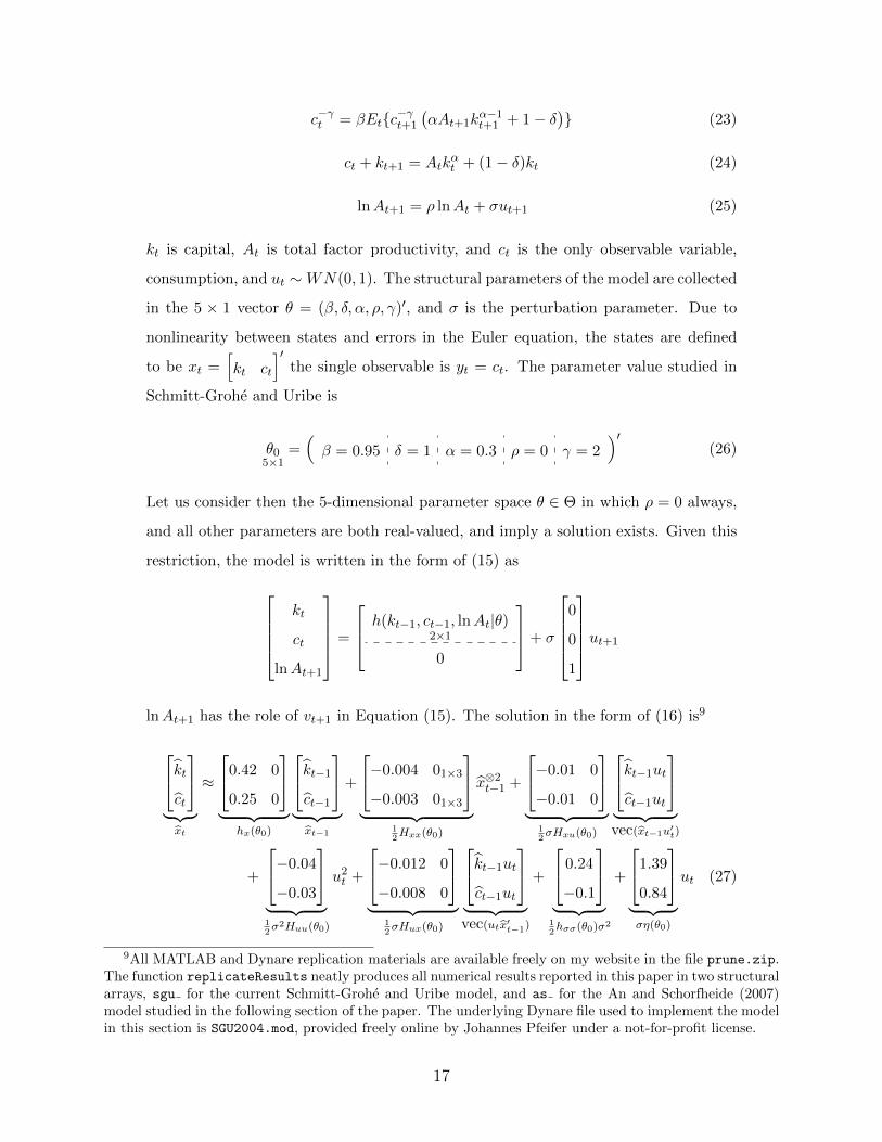
16
c−γt = βEt{c−γt+1
(αAt+1k
α−1t+1 + 1− δ
)} (23)
ct + kt+1 = Atkαt + (1− δ)kt (24)
lnAt+1 = ρ lnAt + σut+1 (25)
kt is capital, At is total factor productivity, and ct is the only observable variable,
consumption, and ut ∼WN(0, 1). The structural parameters of the model are collected
in the 5 × 1 vector θ = (β, δ, α, ρ, γ)′, and σ is the perturbation parameter. Due to
nonlinearity between states and errors in the Euler equation, the states are defined
to be xt =[kt ct
]′the single observable is yt = ct. The parameter value studied in
Schmitt-Grohe and Uribe is
θ05×1
=(β = 0.95 δ = 1 α = 0.3 ρ = 0 γ = 2
)′(26)
Let us consider then the 5-dimensional parameter space θ ∈ Θ in which ρ = 0 always,
and all other parameters are both real-valued, and imply a solution exists. Given this
restriction, the model is written in the form of (15) as
kt
ct
lnAt+1
=
h(kt−1, ct−1, lnAt|θ)2×1
0
+ σ
0
0
1
ut+1
lnAt+1 has the role of vt+1 in Equation (15). The solution in the form of (16) is9
ktct
︸ ︷︷ ︸xt
≈
0.42 0
0.25 0
︸ ︷︷ ︸
hx(θ0)
kt−1
ct−1
︸ ︷︷ ︸xt−1
+
−0.004 01×3
−0.003 01×3
︸ ︷︷ ︸
12Hxx(θ0)
x⊗2t−1 +
−0.01 0
−0.01 0
︸ ︷︷ ︸
12σHxu(θ0)
kt−1ut
ct−1ut
︸ ︷︷ ︸vec(xt−1u′t)
+
−0.04
−0.03
︸ ︷︷ ︸12σ2Huu(θ0)
u2t +
−0.012 0
−0.008 0
︸ ︷︷ ︸
12σHux(θ0)
kt−1ut
ct−1ut
︸ ︷︷ ︸vec(utx′t−1)
+
0.24
−0.1
︸ ︷︷ ︸12hσσ(θ0)σ2
+
1.39
0.84
︸ ︷︷ ︸ση(θ0)
ut (27)
9All MATLAB and Dynare replication materials are available freely on my website in the file prune.zip.The function replicateResults neatly produces all numerical results reported in this paper in two structuralarrays, sgu for the current Schmitt-Grohe and Uribe model, and as for the An and Schorfheide (2007)model studied in the following section of the paper. The underlying Dynare file used to implement the modelin this section is SGU2004.mod, provided freely online by Johannes Pfeifer under a not-for-profit license.
17
and the observation equation is merely an identity.
ct︸︷︷︸yt
=[0 1
]︸ ︷︷ ︸gx(θ0)
xt + 01×9︸︷︷︸
12Gxx(θ0)
x⊗2t + 0︸︷︷︸
12gσσ(θ)σ2
(28)
The zeros in hx and Hxx arise due to the fact that TFP is not persistent, ρ = 0. Since
we are considering the parameter space Θ in which ρ = 0 always, Assumption 2 is
satisfied. In order to simplify the model at hand to ABCD representation, I now use
the three-step methodology described in Appendix C.
Step 1. The pruned model may be represented by the rule of motion
Zt = J(θ0) + P (θ0)Zt−1 +R(θ0)Ut (29)
Yt = S(θ0)Zt (30)
where J , P , and R correspond to the expressions given previously in (19) and (20).
4 φ Index of price stckness Yt Nom. detr. output5 γ Avg. gr. rate of prod. Πt Inflation
6 Π St. state level of infl. Ct Nom. detr. cons.7 G St. state level of Gt.8 ψπ Taylor rule infl. coeff.9 ψy Taylor rule out. coeff.10 ρz zt persistence11 ρg gt persistence12 ρr rt persistence13 σz εzt std error14 σg εgt std error15 σr εrt std error
Table 1: An and Schorfheide (2007) model parameter and variable names.
vector ut = [uzt, ugt, urt]′ is distributed as ut ∼ WN(0, I3). In all, there are six
equilibrium conditions (36) - (41) which completely characterize equilibrium for this
model stated in terms of the six (detrended) variables of interest lnZt, lnGt, lnRt,
ln Yt = ln(Yt/At), ln Πt, and ln Ct = ln(Ct/At) along with the shocks. Henceforth,
these total nine variables will be collected in the following vectors, where vt is the
ancillary parameter for models with nonlinearities in errors and shocks defined in (15).
[x′t−1 v′t
]′(6×1)
=[lnZt−1 lnGt−1 lnRt−1 εzt εgt εrt
]′(42)
yt(3×1)
=[lnRt ln Yt ln Πt
]′(43)
With these definitions in mind, the equilibrium equations may also be represented
concisely in the form of Equation (1). Thus, the solution will have the form of Equations
(2) and (15). Define h(3) to be the third row of h. Then the state equation may be
26
expressed as
lnZt
lnGt
lnRt
εzt+1
εgt+1
εrt+1
︸ ︷︷ ︸[x′t v
′t+1]′
=
ρz lnZt−1 + εzt
ρg lnGt−1 + εgt
h(3)(xt−1, vt, σ|θ)
0
0
0
+ σ
03×3σz · ·
0 σg ·
0 0 σr
︸ ︷︷ ︸
Lu(θ)
︸ ︷︷ ︸
η(θ)
uzt+1
ugt+1
urt+1
︸ ︷︷ ︸ut+1
(44)
Definining g(i) to be the i-th row of g, the observation equation may be written
lnRt
ln Yt
ln Πt
︸ ︷︷ ︸
yt
=
lnRt
g(2)(xt, σ|θ)
g(3)(xt, σ|θ)
︸ ︷︷ ︸
g(xt,σ|θ)
(45)
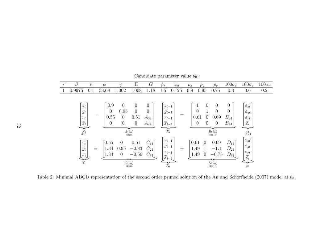
Solving the model and using the same 3-step procedure given in Appendix C and
demonstrated in the context of the Schmitt-Grohe and Uribe model in Section 3 .3
yields the minimal ABCD representation in Table 2.11 zt, gt, and rt are first-order
approximations of TFP, government spending, and interest rates. Second-order terms
are collected into the 5× 1-dimensional xt and 13× 1-dimensional εt. The elements of
xt contain a demeaned transformation of the 5 state cross-products
xt : z2t , gtzt, rtzt, rtgt, r
2t
This includes all unique cross-products of the minimal state vector for the linearized
model, excluding g2t . g2
t is not part of the minimal state vector because the micro-
foundations imply the corresponding column in Hxx is zero in the entirety of Θ. The
elements of εt contain a demeaned transformation of the 13 cross-products of states
11Explicit forms for the block elements {Aij , Bij , Cij , Dij}, as well as the observability and controllabilitymatrices, are output by the function replicateResults into the structural array as . All block-elements ofthe state space are of conformable dimension to corresponding states and errors. For instance, A34 is 1× 5,A44 is 5× 5, B34 is 1× 13, and B44 is 5× 13. The 8× 24 dimensional controllability matrix as .CON is fullrow rank, and the 24× 8 dimensional observability matrix as .OBS is full column rank, verifying minimality.
27
and errors
εt : all of vec
zt−1
gt−1
rt−1
εzt
εgt
εrt
′ except gt−1εgt and vech
εzt
εgt
εrt
εzt
εgt
εrt
′ except ε2
gt.
Compare the ABCD representation in Table 2 with the minimal ABCD represen-
tation of the linearized version of the same model at θ0 in Komunjer and Ng (2011)
Table 1. Similarly to our observation regarding the Schmitt-Grohe and Uribe model,
in this case, it is quite clear that the linear model is nested within the nonlinear ap-
proximation. Indeed, the second order elements of the minimal Xt and εt for the
model in Table 2 are simply functions of the minimal state vector and shocks from first
order representation. Given these observations, and the previous enhanced identifia-
bility in Schmitt-Grohe and Uribe’s model, a natural question to ask is whether more
parameters are identifiable in this case as well.
5 .1 Local identifiability
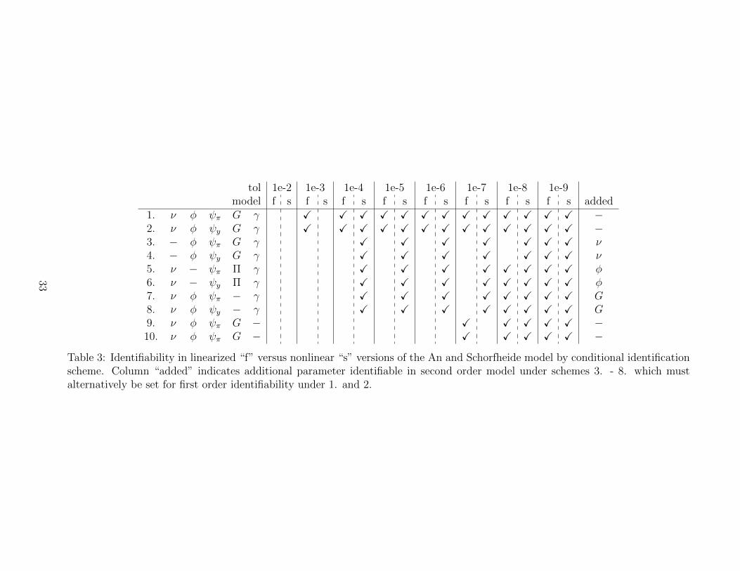
In Table 3 I consider identifiability subject to ten sets of conditional identification
restrictions.12 A conditional identification restriction generally takes the form ϕ(θ) = 0.
Here, as in Komunjer and Ng (2011), these restrictions will take the form of setting
some parameters to constants to identify the complement set. All restrictions I consider
satisfy the necessary order requirement for both linear and nonlinear versions. Rank,
however, is more complicated, due to the fact that ∆(θ0) is large and sparse. ∆ for the
linearized model (nonsingular case) is 42× 33, while for the nonlinear case it expands
to 118 × 79. Therefore, I judge whether the rank condition for ∆ is satisfied for a
range of rank tolerance levels in MATLAB, i.e. minimal tolerated singular value from
the singular value decomposition of ∆. As Komunjer and Ng extensively detail, doing
so not only helps overcome the inherent difficulties with judging the rank of sparse
matrices, but also provides a means for judging the strength of identification.
12The function in the attached documentation to reproduce the content in Table 3 is the functionasTable(n,tol). Input n are the number of conditional identifying restrictions, and tol is the specifiedtolerance for rank evaluation. The output is a table in which each row contains the numerical codes foreach possible iteration of n fixed constants (codes correspond to the parameter position in θ as given inTable 2), followed by the second to last column which gives 0-1 of whether the complement parameters areidentifiable in the linear model, and the last column, which gives 0-1 of whether the complement parametersare identifiable in the nonlinear model.
28
In Table 3’s columns are tolerances for rank ranging from 1e-2 to 1e-9, with check-
marks X indicating that the rank condition is satisfied for either the first-order model
“f” or second-order nonlinear model “s.” Let us first consider schemes 1. and 2., which
were also studied by Komunjer and Ng in the linear case, and in which 5 parameters
are set to constants. I confirm their finding that ∆ is full rank under either identifying
restriction for tolerance levels of 1e-3 or smaller. Note, by definition the rank condition
for smaller tolerances than one already proven successful will also always be successful.
In the case of the nonlinear model, the rank condition is satisfied only for tolerances
of 1e-4 and above. This may possibly be due to the fact that the structural parame-
ters of the nonlinear model are more weakly identified in the nonlinear model versus
linear under 1. and 2. However, more likely is the fact that ∆ is much larger for the
nonlinear model, so there will inherently be small differences in when rank conditions
are satisfied. Only larger differences in under which tolerance the rank condition are
satisfied are necessarily indicative of differences in identifiability.
Consider conditional identification schemes 3. - 10. In all 8 of these cases, only 4
parameters are set to constants; as Komunjer and Ng argue, 5 is the bare minimum
that must be set in the linear case. In 3. and 4. I first relax the previous assumption
that ν, the inverse elasticity of demand, is fixed. Doing so is motivated by An and
Schorfheide (2007)’s observation (p. 122) that the elasticity of demand and price
stickiness φ do not seem to be separately identifiable in a linearized version of their
model, although curvature in the likelihood appears in both directions for the nonlinear
version. Indeed, I find that the rank condition is satisfied beginning again at 1e-4 for
the nonlinear model, but not until the much smaller value of 1e-9 is the rank condition
for the linear model satisfied. As Komunjer and Ng, false positives are likely at this
magnitude. Therefore, the results strongly suggest that ν is identifiable under 3. and
4., in addition to the maximum 10 parameters identifiable in the linear case under 1.
and 2. However, the strength of these now 11 identifiable parameters may be weaker
than the identifiability of the previous 10 under 1. and 2. Intuitively, this result is
supported by the fact that ν and φ are linearly dependent within the Phillips curve
coefficient κ = τ(1− ν)/(νφΠ2) for the linearized model, but ν is linearly independent
in the nonlinear version of the Phillips curve, (36).
Now consider 5. and 6. In both cases I relax the assumption φ is fixed. In no case
is the rank condition satisfied over the ranges of tolerances I consider when G is also
29
free. Therefore I substitute G from the previous schemes with Π. Again I find that
identification is possible in the nonlinear model at only 1e-4, but not linear model, for
which the largest possible tolerance 1e-8 is too small to ensure we have not arrived at
a false conclusion. Therefore, the second part of An and Schorfheide (2007)’s previous
intuition that φ may be identifiable is concerned. Like ν and φ, An and Schorfheide
lastly hypothesize G is identifiable in the nonlinear version of their model, but not
linear (p. 164). In schemes 7. and 8., this rationale is also verified. Finally, in 9.
and 10., I attempt to identify γ by simply relaxing its restriction. In fact, not only
in cases 9. and 10., but in any possible 4 set parameters restriction does γ seem to
be identifiable. Although in the linear model the highest possible tolerance has crept
up to 1e-7, this is still not as unfathomable evidence of identifiability versus simply
numerical difficulty as in the range of 1e-3 to 1e-4.
5 .2 Discussion: A free lunch?
Setting parameters to constants to enhance identifiability is more due to ease than
reason. As in the case of the Schmitt-Grohe and Uribe model, it appears that strictly
more parameters are identifiable in a nonlinear version of An and Schorfheide’s model
than linear, which is promising. An important caveat is that the strength of identifi-
cation may not be as certain as when more parameters are fixed in the linear model.
However, the conclusion that the strength of identification should decrease as more
parameters are let free is not surprising.
In some sense the proven result in this paper is surprising; after all, the observables
utilized in the nonlinear ABCD representation given in Table 2 are exactly those that
are utilized in the linear model. Is it possible that ever-higher approximations can
only assist identifiability? The most sensible explanation seems to be that the higher
order terms of the Taylor model must add curvature to the likelihood surface without
violating the order condition 2nXnY + nY (nY + 1)/2 = 3 < nθ. In the case of the An
and Schorfheide model, the second order terms have evidently added curvature in the
dimensions of ν, φ, and G, without coming near violating the order condition. However,
as the order of approximation increases, so will nX , while nY and nθ remain constant.
So, in all cases, there is a limit to how high order of an approximation. There is more
of a happy middle ground than an unfettered free lunch. The decision of what order is
30
useful is conditional on the model at hand, and may be evaluated by the analyst using
the procedure derived in this paper.
6 Conclusion
In this paper, I have shown how to assess parameter identifiability in nonlinear approx-
imations of DSGE models. Due to the inherent nestedness of Taylor approximations,
nonlinear approximations of these models may be used to identify key parameters of
interest that are otherwise not identifiable from a linear approximation. In the con-
text of the An and Schorfheide (2007) model, I have shown this to be true for three
important parameters, the elasticity of substitution, price stickiness, and steady state
level of government spending. Unanswered questions remain whether the strength of
identification is always weaker when parametric restrictions are relaxed, and whether
nonlinear approximations help address the issue of global identifiability described in
Morris (2014). I leave this questions for further research.
Table 2: Minimal ABCD representation of the second order pruned solution of the An and Schorfheide (2007) model at θ0.
32
tol 1e-2 1e-3 1e-4 1e-5 1e-6 1e-7 1e-8 1e-9model f s f s f s f s f s f s f s f s added
1. ν φ ψπ G γ X X X X X X X X X X X X X −2. ν φ ψy G γ X X X X X X X X X X X X X −3. − φ ψπ G γ X X X X X X X ν4. − φ ψy G γ X X X X X X X ν5. ν − ψπ Π γ X X X X X X X X φ6. ν − ψy Π γ X X X X X X X X φ7. ν φ ψπ − γ X X X X X X X X G8. ν φ ψy − γ X X X X X X X X G9. ν φ ψπ G − X X X X X −10. ν φ ψπ G − X X X X X −
Table 3: Identifiability in linearized “f” versus nonlinear “s” versions of the An and Schorfheide model by conditional identificationscheme. Column “added” indicates additional parameter identifiable in second order model under schemes 3. - 8. which mustalternatively be set for first order identifiability under 1. and 2.
33
References
Abadir, K. M. and J. R. Magnus (2005): Matrix Algebra, Cambridge University
Press.
Amisano, G. and O. Tristani (2010): “Euro Area Inflation Persistence in an Es-
timated Nonlinear DSGE Model,” Journal of Economic Dynamics and Control, 34,
1837–1858.
An, S. and F. Schorfheide (2007): “Bayesian Analysis of DSGE Models,” Econo-
metric Reviews, 26, 113–172.
Andreasen, M. M., J. Fernandez-Villaverde, and J. Rubio-Ramırez (2014):
“The Pruned State-Space System for Non-Linear DSGE Models: Theory and Em-
pirical Applications,” NBER Working Paper Series, Working Paper 18983.
Andrews, I. and A. Mikusheva (2014): “Maximum Likelihood Inference in Weakly
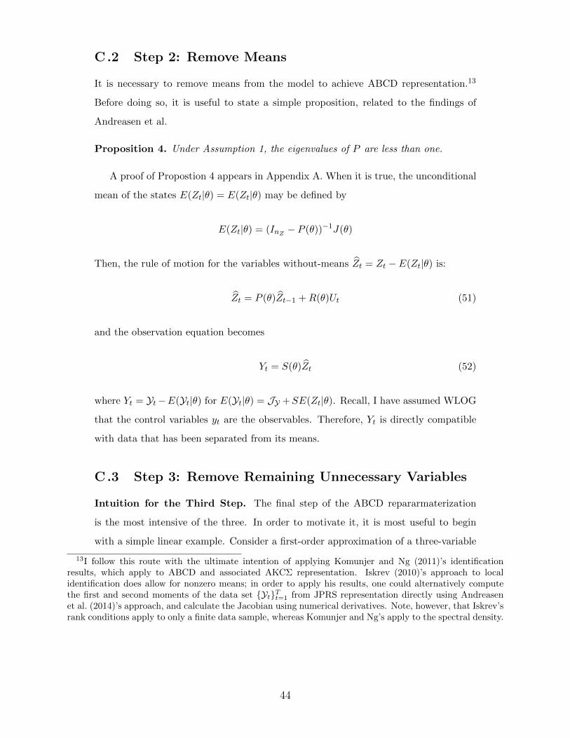
Intuition for the Third Step. The final step of the ABCD repararmaterization
is the most intensive of the three. In order to motivate it, it is most useful to begin
with a simple linear example. Consider a first-order approximation of a three-variable
13I follow this route with the ultimate intention of applying Komunjer and Ng (2011)’s identificationresults, which apply to ABCD and associated AKCΣ representation. Iskrev (2010)’s approach to localidentification does allow for nonzero means; in order to apply his results, one could alternatively computethe first and second moments of the data set {Yt}Tt=1 from JPRS representation directly using Andreasenet al. (2014)’s approach, and calculate the Jacobian using numerical derivatives. Note, however, that Iskrev’srank conditions apply to only a finite data sample, whereas Komunjer and Ng’s apply to the spectral density.
44
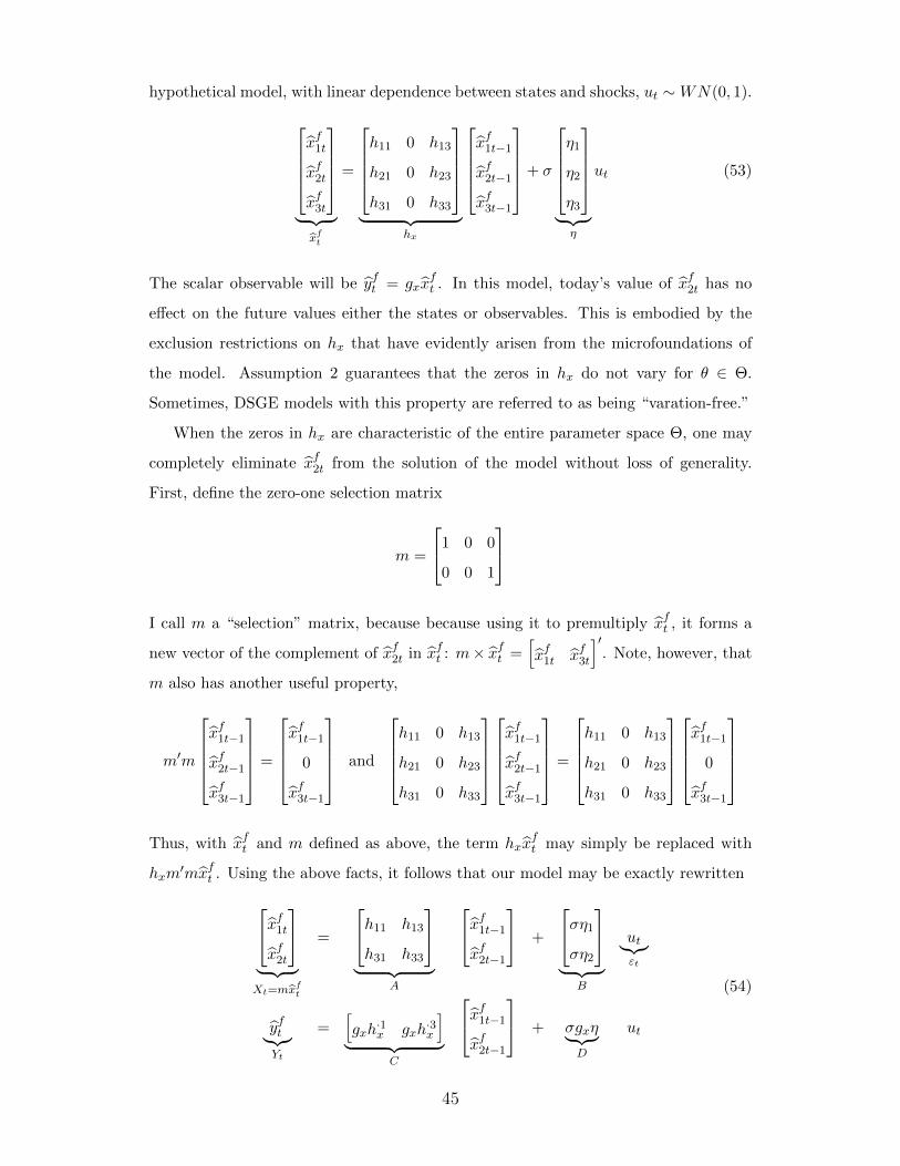
hypothetical model, with linear dependence between states and shocks, ut ∼WN(0, 1).
xf1t
xf2t
xf3t
︸ ︷︷ ︸xft
=
h11 0 h13
h21 0 h23
h31 0 h33
︸ ︷︷ ︸
hx
xf1t−1
xf2t−1
xf3t−1
+ σ
η1
η2
η3
︸ ︷︷ ︸η
ut (53)
The scalar observable will be yft = gxxft . In this model, today’s value of xf2t has no
effect on the future values either the states or observables. This is embodied by the
exclusion restrictions on hx that have evidently arisen from the microfoundations of
the model. Assumption 2 guarantees that the zeros in hx do not vary for θ ∈ Θ.
Sometimes, DSGE models with this property are referred to as being “varation-free.”
When the zeros in hx are characteristic of the entire parameter space Θ, one may
completely eliminate xf2t from the solution of the model without loss of generality.
First, define the zero-one selection matrix
m =
1 0 0
0 0 1
I call m a “selection” matrix, because because using it to premultiply xft , it forms a
new vector of the complement of xf2t in xft : m× xft =[xf1t xf3t
]′. Note, however, that
m also has another useful property,
m′m
xf1t−1
xf2t−1
xf3t−1
=
xf1t−1
0
xf3t−1
and
h11 0 h13
h21 0 h23
h31 0 h33
xf1t−1
xf2t−1
xf3t−1
=
h11 0 h13
h21 0 h23
h31 0 h33
xf1t−1
0
xf3t−1
Thus, with xft and m defined as above, the term hxx
ft may simply be replaced with
hxm′mxft . Using the above facts, it follows that our model may be exactly rewritten
xf1txf2t
︸ ︷︷ ︸Xt=mx
ft
=
h11 h13
h31 h33
︸ ︷︷ ︸
A
xf1t−1
xf2t−1
+
ση1
ση2
︸ ︷︷ ︸
B
ut︸︷︷︸εt
yft︸︷︷︸Yt
=[gxh·1x gxh
·3x
]︸ ︷︷ ︸
C
xf1t−1
xf2t−1
+ σgxη︸ ︷︷ ︸D
ut
(54)
45
where A = mhxm′, B = σmη, C = gxhxm
′, and D is as expressed above. h·ix denotes
the entire i-th column of hx. The dimensions of the state, observables, and innovations
are denoted nX = 2, nY = 1, and nε = 1. This is known as the ABCD representation
of the model.
As Komunjer and Ng (2011) point out, not only does this process of removing
states on the basis of exclusion restrictions reduce the dimension of the state vector
for linearized DSGE models, but typically, the remaining state vector mxft is minimal.
Since it is easy to use the selection matrix m to obtain minimal ABCD representation
of linearized models, a natural question is whether a similar procedure may be used
for the class of pruned nonlinear models currently under consideration. This is Step 3.
The Third Step. Consider the pruned second order solution of the same hypothetical
model presented in Equation (53). Note, due to the nested nature of Taylor approxi-
mations, exactly the same hx is nested in this solution (Compare with equation (11)).
xs1t
xs2t
xs3t
︸ ︷︷ ︸xst
=
h11 0 h13
h21 0 h23
h31 0 h33
︸ ︷︷ ︸
hx
xs1t−1
xs2t−1
xs3t−1
+1
2
H1 0 H13 0 0 H16
H21 0 H23 0 0 H26
H31 0 H33 0 0 H36
︸ ︷︷ ︸
12HxxDnx
xf21t
xf2txf1t
xf3txf1t
xf22t
xf3txf2t
xf23t
︸ ︷︷ ︸D+nx x
ft
+1
2hσσσ
2
Zeros on the first order coefficients often imply zeros on the second order coefficients
for the same variable; for intuition, consider the hypothetical process x2t = αx1t−1 +εt.
This explains the location of zeros in Hxx in comparison to the zeros in hx. Returning
to Step 2, the representation without-means expression Equation (51) for the states is
xft
Z2t
Z3t
︸ ︷︷ ︸Zt
=
hx 0 0
0 hx12HxxDnx
0 0 D+nxh⊗2x Dnx
︸ ︷︷ ︸
P
xft−1
Z2t−1
Z3t−1
+
ση 0 0
0 0 0
0 σ2D+nxη⊗2Dnu σr(θ)
︸ ︷︷ ︸
R
ut
u2t − 1
xft ut
︸ ︷︷ ︸
Ut
Where Z2t is an nx × 1 vector of the second order solution states separated from
their means, Z2t = xst − E(xst |θ0) and Z3t is the nx(nx + 1)/2 × 1 mean-zero vector
46
D+nx x
st − E(D+
nx xst |θ0). The observation equation is the following; Yt = yft + yst −
12gσσσ
2 − SE(Zt|θ) is a scalar:
Yt =[gx gx
12GxxDnx
]︸ ︷︷ ︸
S
Zt
The selection matrix m was previously used in the linear case to select a subvector of xft
corresponding to the non-zero columns of hx. Within P , however, there are zeros not
only in the submatrix hx, but also the submatrices 12HxxDnx and D+
nxh⊗2x Dnx . Thus,
defining a similar selection matrix for this case requires a slightly different strategy.
First, drawing on the theme of nestedness of progressively higher-order solutions, note
that the only submatrix of P premultiplying Zt−1 is again hx. Thus, with m exactly
as previously defined, mZ2t−1 is the 3 × 1 vector that selects only the 3 elements of
the 6-dimensional vector Z2t−1 that correspond to non-zero columns in hx. Second, we
have the fact that there are zeros in the second, fourth, and fifth columns of 12HxxDnx
as displayed above. But in addition, note that
D+nxh⊗2x Dnx
6×6
=
h211 0 h11h13 0 0 h2
13
h11h21 0 h11h23 0 0 h13h23
h11h31 0 h11h33 0 0 h13h33
h221 0 h21h23 0 0 h2
23
h21h31 0 h21h33 0 0 h23h33
h231 0 h31h33 0 0 h2
33
So, only the second, fourth, and fifth columns of both 1
2HxxDnx and D+nxh⊗2x Dnx have
zeros. For this reason define
m∗ =
1 0 0 0 0 0
0 0 1 0 0 0
0 0 0 0 0 1
Then, m∗Z3t−1 is the 3×1 vector that selects only the 3 elements of the 6-dimensional
vector Z3t−1 that correspond to non-zero columns in 12HxxDnx and D+
nxh⊗2x Dnx , and
m∗′mZ3t−1 replaces the appropriate elements with zeros (recall the operations of m′m
47
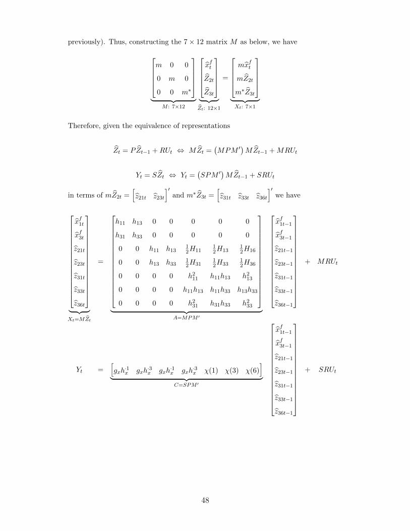
previously). Thus, constructing the 7× 12 matrix M as below, we have
m 0 0
0 m 0
0 0 m∗
︸ ︷︷ ︸
M : 7×12
xft
Z2t
Z3t
︸ ︷︷ ︸Zt: 12×1
=
mxft
mZ2t
m∗Z3t
︸ ︷︷ ︸Xt: 7×1
Therefore, given the equivalence of representations
Zt = PZt−1 +RUt ⇔ MZt =(MPM ′
)MZt−1 +MRUt
Yt = SZt ⇔ Yt =(SPM ′
)MZt−1 + SRUt
in terms of mZ2t =[z21t z23t
]′and m∗Z3t =
[z31t z33t z36t
]′we have
xf1t
xf3t
z21t
z23t
z31t
z33t
z36t
︸ ︷︷ ︸Xt=MZt
=
h11 h13 0 0 0 0 0
h31 h33 0 0 0 0 0
0 0 h11 h1312H11
12H13
12H16
0 0 h13 h3312H31
12H33
12H36
0 0 0 0 h211 h11h13 h2
13
0 0 0 0 h11h13 h11h33 h13h33
0 0 0 0 h231 h31h33 h2
33
︸ ︷︷ ︸
A=MPM ′
xf1t−1
xf3t−1
z21t−1
z23t−1
z31t−1
z33t−1
z36t−1
+ MRUt
Yt =[gxh·1x gxh
·3x gxh
·1x gxh
·3x χ(1) χ(3) χ(6)
]︸ ︷︷ ︸
C=SPM ′
xf1t−1
xf3t−1
z21t−1
z23t−1
z31t−1
z33t−1
z36t−1
+ SRUt
48
where
χ(i) denotes gx ×(
the i-th column of1
2HxxDnx
)+
1
2GxxDnx ×
(the i-th column of D+
nxh⊗2x Dnx
)There is one last substep to reduce the dimension of the errors. Recall, the matrix R is
a function of hxx through its submatrix r. Therefore, zeros in hxx will imply elements
of Ut may be shed, just as elements of Zt may be. To see this in the current ongoing
example, and recalling that r = D+nx (η ⊗ hx + (hx ⊗ η)Knx,nu), then r has the form
r6×3
=
2η1h11 0 2η1h13
η3h11 + η1h21 0 η3h13 + η1h23
η3h11 + η1h31 0 η3h13 + η1h33
2η3h21 0 2η3h23
η3(h21 + h31) 0 η3(h23 + h33)
2η3h31 0 2η3h33
Since r premultiplies xft−1ut =[xf1t−1ut xf2t−1ut xf3t−1ut
]′, it is evident how the zeros
in hxx corresponding to xf2t have also translated to zeros in r corresponding to xf2tut.
Thus, recalling how m was originally constructed, and defining another zero-one matrix
n =
1 0 0
0 0 1
→ n′n
xf1t−1ut
xf2t−1ut
xf3t−1ut
=
xf1t−1ut
0
xf3t−1ut
and r
xf1t−1ut
xf2t−1ut
xf3t−1ut
= r
xf1t−1ut
0
xf3t−1ut
And using n, define N to be
N =
1 0 0
0 1 0
0 0 n
we ultimately obtain the further reduced representation
49
xf1t
xf3t
z21t
z23t
z31t
z33t
z36t
︸ ︷︷ ︸Xt=MZt
= A
xf1t−1
xf3t−1
z21t−1
z23t−1
z31t−1
z33t−1
z36t−1
+
ση1 0 0 0
ση3 0 0 0
0 0 0 0
0 0 0 0
0 η21 2η1h11 2η1h13
0 η1η3 η3h11 + η1h31 η3h13 + η1h33
0 η23 2η3h31 2η3h33
︸ ︷︷ ︸
B=MRN ′
ut
u2t − 1
xf1tut
xf3tut
︸ ︷︷ ︸εt=NUt
Yt = C
xf1t−1
xf3t−1
z21t−1
z23t−1
z31t−1
z33t−1
z36t−1
+
[σgxη
σ2
2 Gxxη⊗2Dnx σψ(1) σψ(3)
]︸ ︷︷ ︸
D=SRN ′
ut
u2t − 1
xf1tut
xf3tut
︸ ︷︷ ︸εt=NUt
where
ψ(i) =1
2GxxDnx × (the i-th column of r)
In other words, we now have ABCD representation, with all unnecessary variables in
Zt and Ut eliminated from the system, and Step 3 is completed. In conclusion, under
Assumptions 1, 2, and 3, the pruned state space model Equations (13) and (14) may
be written in terms of deviations from mean as an ABCD model
Xt = A(θ) Xt−1 + B(θ) εt
Yt = C(θ) Xt−1 + D(θ) εt(55)
where Xt = MZt, εt = NUt, A = MPM ′, B = MRN ′, C = SPM ′, and D = SRN ′
where Zt = Zt− (InZ −P )−1K for Zt, Ut, K, P , R, and S defined as in Equations (49)
50
and (50) and M and N have the functional form
M =
m 0 0
0 m 0
0 0 m∗
N =
Inu 0 0
0 Inu(nu+1)/2 0
0 0 n
with the submatrices m, m∗, and n being defined appropriately for the model at hand
to eliminate all unnecessary elements of Zt and Ut. Corollary 1, that εt is white noise,
in a consequence of the fact that ut is white noise, and is described in Appendix A.
D Definitions
Definition 1. Controllability: For every θ ∈ Θ, define the controllability matrix by
C(θ) =(B(θ) A(θ)B(θ) . . . A(θ)nX−1B(θ)
)We say {A(θ), B(θ)} is controllable if and only if C(θ) is full row rank.
Definition 2. Observability: For every θ ∈ Θ, define the observability matrix by
O(θ) =(C(θ)′ A(θ)′C(θ)′ . . . A(θ)nX−1′C(θ)′
)′We say {A(θ), C(θ)} is observable if and only if O(θ) is full column rank.
Definition 3. Minimality: {A(θ), B(θ), C(θ), D(θ)} is called minimal if and only if
{A(θ), B(θ)} is controllable and {A(θ), C(θ)} is observable (Kailath et al. (2000) p.
765).
Definition 4. Stochastic Singularity: ABCD representation is stochastically singu-
lar (“singular”) if nε ≤ nY . If nε ≥ nY , the model is called stochastically nonsingular
(“nonsingular”), and if nε = nY the model is therefore both singular and nonsingular.
E Generalization to Higher Order Models
Andreasen et al. (2014) show that third order pruned state space representation also
has JPRS representation. I claim but leave for verification in further research that the
51
above steps may be replicated almost exactly to obtain minimal ABCD or AKCΣ repre-
sentation of these models. The only additional tool that is required is Meijer (2005)’s
triplication and quadruplication matrices used in place of the duplication matrix in
Step 1 of the 3-Step ABCD reparameterization. Recall, the duplication matrix has
the property of equating x⊗2t to its unique elements only by the equality x⊗2
t = Dnx ×
(unique elements of x⊗2t ) (The unique elements of x⊗2
t are also vech(xtx′t)). The Moore-
Penrose inverse D+nx = (D′nxDnx)−1D′nx equates (un. el. of x⊗2
t ) = D+nxx⊗2t . The trip-
lication matrix Tnx has the property x⊗3t = Tnx × (un. el. of x⊗3
t ) and T+nx exists.
The quadruplication matrix Qnx has the property that x⊗4t = Qnx × (un. el. of x⊗4
t )
and Q+nx exists. These matrices and the steps above may be used to obtain minimal
representation of third order models. Meijer also provides higher-order n-tuplication
matrices that could be used or those interested in fourth or higher order models.