Physica C 480 (2012) 55–60

Contents lists available at SciVerse ScienceDirect

Physica C

journal homepage: www.elsevier .com/locate /physc

Localization–delocalization transition in a two-dimensionalHolstein–Hubbard model

I.V. Sankar a, Soma Mukhopadhyay b, Ashok Chatterjee a,⇑a School of Physics, University of Hyderabad, Hyderabad 500 046, Indiab Department of Physics, DVR College of Engineering and Technology, Kashipur, Sangareddy Mandal, Hyderabad 502 285, India

a r t i c l e i n f o a b s t r a c t

Article history:Received 17 April 2012Received in revised form 30 April 2012Accepted 10 May 2012Available online 29 May 2012

Keywords:Holstein–Hubbard modelHartree–Fock approximationSelf-trapping transitionLarge polaronSmall polaron

0921-4534/$ - see front matter � 2012 Elsevier B.V. Ahttp://dx.doi.org/10.1016/j.physc.2012.05.004

⇑ Corresponding author. Tel.: +91 40 23134356.E-mail address: acsp@uohyd.ernet.in (A. Chatterje

The nature of self-trapping transition is investigated within the framework of an extended Holstein–Hubbard model in two dimensions using a variational method. We perform a series of canonical trans-formations including phonon coherence effect that partly depends on the electron density and is partlyindependent and also the effect of on-site and nearest-neighbor phonon correlations to obtain an effec-tive extended Hubbard model which is finally studied using the mean-field Hartree–Fock approximation.The mean-field solution of the effective extended Hubbard model suggests that the transition from thelarge polaron state to a small polaron state in the anti-adiabatic regime is continuous, while in theadiabatic limit it predicts a discontinuous transition.

� 2012 Elsevier B.V. All rights reserved.

1. Introduction

A conduction electron in an ionic solid is known to deform thelattice in its vicinity forming a quasi-particle called polaron (forreview [1]). In the weak electron–phonon coupling regime, thedistortion of the lattice spreads over several lattice points andthe lattice polarization potential created by the electron is shallowand as a result the polaron becomes delocalized and one is thensaid to have a mobile large polaron. On the contrary, if the interac-tion between the electron and the lattice vibrations is reasonablystrong, the lattice distortion might be essentially restricted withinone lattice spacing and then the lattice polarization potentialwould be deep enough to trap the electron and the correspondingpolaron is referred to as a localized small polaron. This is the con-ventional Landau–Pekar problem. However, it is also possible thateven at strong-coupling the lattice distortion may extend overmany lattice sites, so that one has a small Froehlich polaron withthe extended distortion but a small size of the electron wave func-tion [2]. It has been theoretically established that as the electron–phonon coupling is increased, at some critical value of the couplingconstant a large polaron transforms into a small polaron which isoften referred as a self-trapping (ST) transition. In the Fröhlichmodel, it has been shown using the Feynman path-integral methodthat this transition, albeit rapid, is continuous [3]. However, in atight-binding scenario, i.e. in a small polaron model, which is a

ll rights reserved.

e).

proper framework for a correlated system, there is, in general, noclear consensus on the nature of this crossover. This issue has beenthe subject of extensive investigations in the last few decades. Inview of the potential role of small polarons in high Tc superconduc-tors [4,5] and colossal magneto-resistance materials [6], it iscertainly more important to understand the nature of the ST tran-sition in small polaron models. In fact, the phase transition prob-lem in a small polaron system was studied long ago byToyozawa [7]. Toyozawa and collaborators [7] have studied thesmall polaron problem in the adiabatic approximation and haveobtained a discontinuous phase transition. Several other authors[8] have obtained similar abrupt changes in the polaron propertieswhereas quite a few investigations [9,10] have also shown contin-uous transition. Löwen [10] has investigated the exact nature ofthe phase transition for the small polaron problem within theframework of the Holstein model [11] and has shown that for finitephonon frequencies the ground state of an electron–phonon sys-tem does not exhibit any non-analytical phase transition as thephonon coupling increases. It thus appears that the discontinuitiesin the polaron properties obtained by various authors might ratherbe consequences of the approximations used. The analysis ofLöwen however does not rule out the possibility of a large changein the polaronic properties in the adiabatic limit and furthermore itdeals with a single electron only. Therefore the issue of the ST tran-sition in the case of a many-small polaron system still remains animportant open problem. In fact there have been suggestions [6]advocating essentially the ST transition as the basic mechanismfor the large increase in magneto-resistance associated with the

56 I.V. Sankar et al. / Physica C 480 (2012) 55–60

paramagnetic–ferromagnetic phase transition in manganites andin this context, the study of the Holstein–Hubbard (HH) model be-comes particularly more important. Krishna et al. [12] have studiedthe nature of the self-trapping transition in a one-dimensional HHmodel where it has been shown almost conclusively that this tran-sition is continuous. However the nature of the self-trapping tran-sition is more important in higher dimensions. Das and Sil [13]have studied the ST transition for a many-polaron system in thetwo-dimensional (2D) HH model. Using a modified Lang–Firsov(LF) transformation [13,14] and a two-phonon coherent state forthe phonons [15] and a Hartree–Fock (HF) decoupling scheme forthe electronic correlation term, they have shown that the crossoverfrom the large polaron to a small polaron regime is continuous inthe anti-adiabatic case, whereas in the adiabatic case discontinu-ous jumps appear in the polaron properties. They have attributedthe discontinuity observed at the cross-over region to the insuffi-cient number of parameters used in the trial variational wave func-tion. In view of the importance of the ST transition in manganites,high Tc – superconductors, semiconductor nanostructures andother materials, we believe that a more careful investigation ofthe ST transition in the 2D HH model is certainly called for andthe purpose of the present paper is to make an attempt in thisdirection. In the present paper we shall purport to suggest a muchbetter variational wave function to carry out a more rigorousinvestigation on the nature of the ST transition in the extendedHH (EHH) model.

2. The model

The extended Holstein–Hubbard model may be written as:

H ¼ �Xhijir

tijcyircjr þ U

Xi

ni"ni# þx0

Xi

byi bi þ V1

Xhijirr0

nirnjr0

þ V2

Xid0rr0

nirniþd0 ;r0 þ V3

Xid00rr0

nirniþd00 ;r0 þ g1

Xir

nirðbi þ byi Þ

þ g2

Xidr

nirðbiþd þ byiþdÞ ð1Þ

where the first term represents the kinetic energy of the localizedelectron with tij as the bare hopping integral, cyir (cir) the creation(annihilation) operator for an electron with spin r at the i-th latticesite. The notation hiji in the hopping term denotes that the summa-tion over i and j has to be carried over nearest-neighbors only andwe shall take tij = t for the sake of simplicity. The second term isthe on-site Coulomb interaction with U as the strength of the inter-action and nir (=cyircir) the electron number operator. The third termis the non-interacting phonon Hamiltonian, x0 being the disper-sionless optical phonon frequency and byi (bi) the phonon creation(annihilation) operator at the i-th lattice site. The fourth, fifth andthe sixth terms are nearest-neighbor (NN), next NN (NNN) and nextNNN Coulomb interactions with V1, V2 and V3 giving the corre-sponding interaction strengths and d, d0 and d00 referring to NN, nextNN and next NNN sites respectively. The last two terms denote theon-site and the NN electron–phonon interactions respectively withg1 and g2 as the corresponding strengths.

3. Formulation

To obtain a variational solution of (1), we perform a series ofcanonical transformations, the first being the modified LF transfor-mation [13,14] with the generator:

R1 ¼g01x0

Xir

nirðbyi � biÞ þg02x0

Xidr

nirðbyiþd � biþdÞ; ð2Þ

where g01 and g02 are variational parameters which give the latticedisplacements created around an electron at the same site and

the NN sites respectively. Thus g01 gives a measure of depth of thepolarization potential, while g02 gives the spread of the lattice defor-mation. In the conventional LF approach, one would choose g01 ¼ g1

and g02 ¼ g2 and obtain the ground state (GS) energy of the systemby averaging the transformed Hamiltonian with respect to a zero-phonon state which however would be good enough approximationfor a strong electron–phonon interaction. In the weak and interme-diate coupling regions, however, a lower GS energy can be obtainedby optimizing g01 and g02. Furthermore, LF transformation assumesthat the phonon coherence coefficient depends linearly on the elec-tron concentration ni. However, one can also introduce, as shown in[16,17] an nir – independent phonon coherence to lower the energyand that can be achieved by a transformation with a generator:

R2 ¼X

i

hiðbyi � biÞ; ð3Þ

where hi is another variational parameter. We shall assume that allsites are identical so that hi ¼ h8i. If t is sufficiently small, then onehas to look for a better phonon state and following Zheng [15] wenow apply a squeezing transformation with a generator:

R3 ¼ aX

i

ðbibi � byi byi Þ; ð4Þ

where a is the squeezing parameter to be obtained variationally.This transformation takes care of the phonon correlation at a partic-ular site and thus partially includes the electron recoil effect andsecondly, it takes into effect through the choice of the phonon statesome effect of the anharmonic phonons, i.e. the phonon–phononinteractions which indirectly introduces the finite life-time effectsof the phonons and thus incorporates the phonon dynamics in amore realistic way. However, it neglects inter-site phonon correla-tions. Lo and Sollie [18] have suggested a correlated squeezing statethat includes the NN phonon correlations and leads to a furtherlowering of the GS energy. Following Lo and Sollie, we now performan additional unitary transformation with a generator:

R4 ¼12

Xi–j

bijðbibj � byi byj Þ; ð5Þ

where we choose bij = b, when i and j are nearest-neighbors andbij = 0 otherwise. Obviously the last two transformations spoil thecoherence of phonons at the expense of including correlations andintroduce some fluctuations. Therefore, in order to deal with thesefluctuations, we perform another coherent state transformation(CST) to bring back the phonon coherence with a generator:

R5 ¼ DX

i

ðbyi � biÞ; ð6Þ

where D is another variational parameter. Averaging the trans-formed Hamiltonian with respect to the zero-phonon state|0i = Pi|0ii, where the product over i runs over N sites, we then ob-tain the following effective extended Hubbard Hamiltonian:

Heff ¼ �e

Xir

nir� te

X<ij>r

cyircjrþUe

Xi

ni"ni# þþVe1

X<ij>rr0

nirnjr0

þVe2

Xid0rr0

nirniþd0 ;r0 þVe3

Xid00rr0

nirniþd00 ;r0

þNx0e4a

4ðe2bÞ00þ

e�4a

4ðe2bÞ00�

12þh2þDe2að2hM1þDe2aM2Þ

� �;

ð7Þ

where

�e ¼ �1x0½2ðg1g01 þ zg2g02Þ � ðg0

2

1 þ zg02

2 Þ�

� 2ðhþ De2aM1Þ½ðg1 þ zg2Þ � ðg01 þ zg02Þ�; ð8Þ

0 0.5 1 1.5 2 2.5 3 3.5 4

−1.44

−1.42

−1.4

−1.38

−1.36

−1.34

−1.32

−1.3

U ( in units of ω0 )

ε 0 (in

uni

ts o

f ω0 )

Das & Sil ResultPresent Result with g2 = 0

Present Result with g2 = 0.02

Anti−adiabatic

t = 0.5n = 0.3

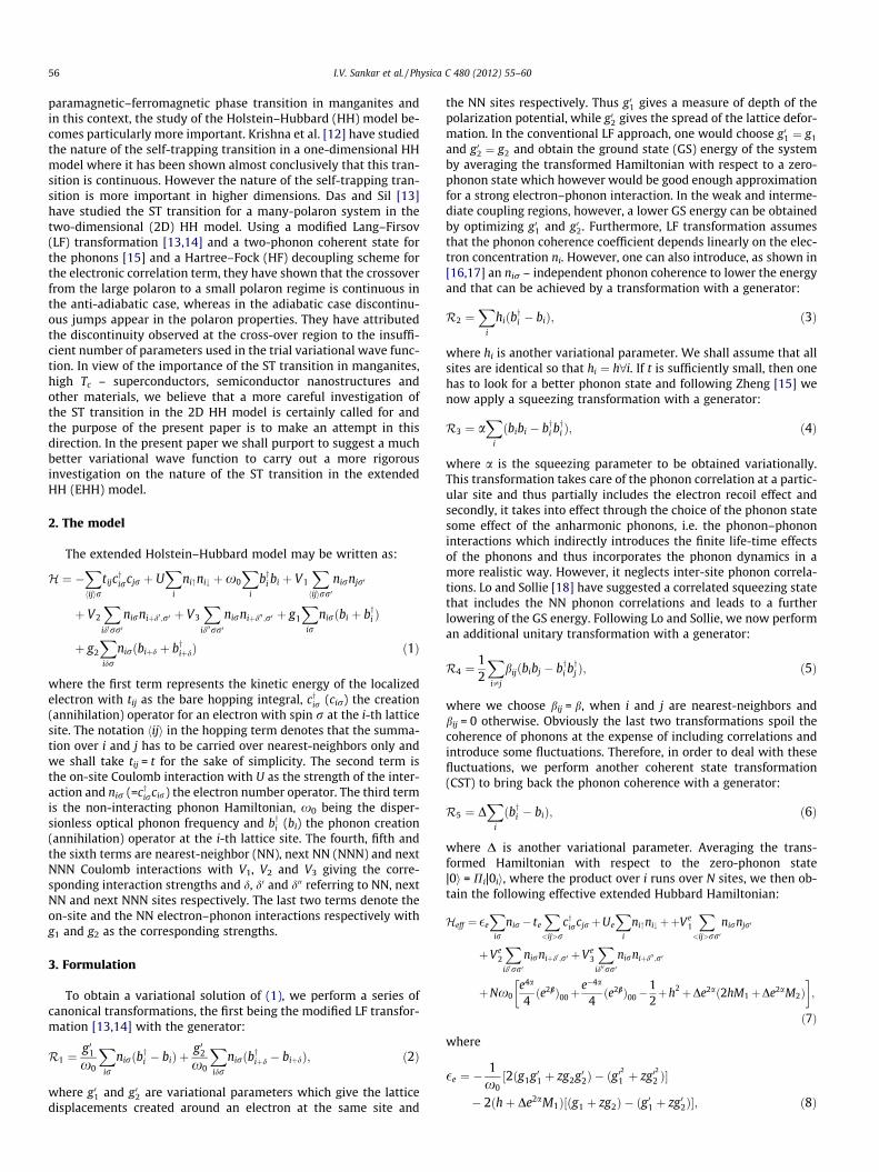
Fig. 1a. e0 vs. U in the anti-adiabatic regime for n = 0.3 and g1 = 0 and 0.02.

0 0.5 1 1.5 2 2.5 3 3.5 4−2.61

−2.57

−2.53

−2.49

−2.45

−2.41

−2.37

U (in units of ω0 )

ε 0 (in

uni

ts o

f ω0 )Das & Sil ResultPresent Result with g

2=0

Present Result with g2

=0.02

Adiabatic

t = 2.0n = 0.3

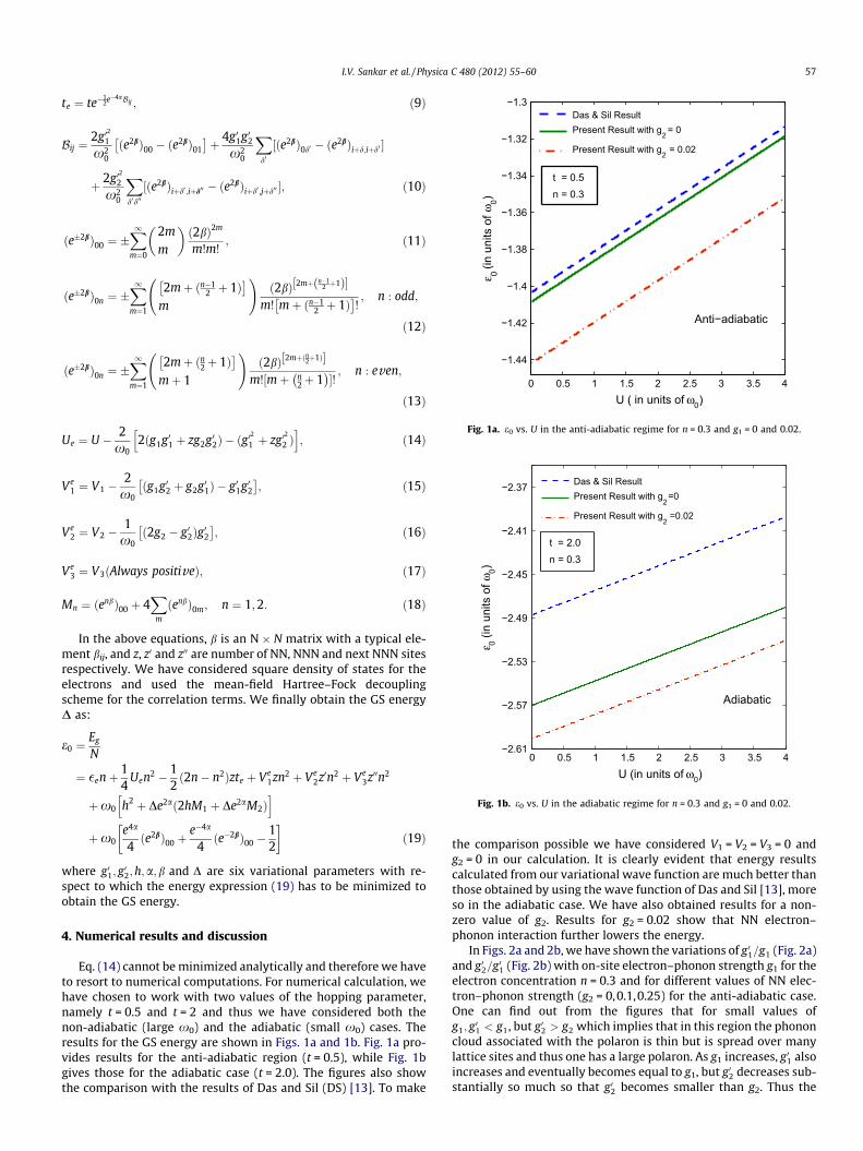
Fig. 1b. e0 vs. U in the adiabatic regime for n = 0.3 and g1 = 0 and 0.02.

I.V. Sankar et al. / Physica C 480 (2012) 55–60 57

te ¼ te�12e�4aBij ; ð9Þ

Bij ¼2g0

2

1

x20

ðe2bÞ00 � ðe2bÞ01

� �þ 4g01g02

x20

Xd0½ðe2bÞ0d0 � ðe2bÞiþd;iþd0 �

þ 2g02

2

x20

Xd0d00½ðe2bÞiþd0 ;iþd00 � ðe2bÞiþd0 ;jþd00 �; ð10Þ

ðe�2bÞ00 ¼ �X1m¼0

2mm

� �ð2bÞ2m

m!m!; ð11Þ

ðe�2bÞ0n ¼ �X1m¼1

2mþ ðn�12 þ 1Þ

� �m

!ð2bÞ 2mþ n�1

2 þ1ð Þ½ �

m! mþ ðn�12 þ 1Þ

� �!; n : odd;

ð12Þ

ðe�2bÞ0n ¼ �X1m¼1

2mþ ðn2þ 1Þ� �mþ 1

!ð2bÞ 2mþðn2þ1Þ½ �

m!½mþ n2þ 1�

�!; n : even;

ð13Þ

Ue ¼ U � 2x0

2ðg1g01 þ zg2g02Þ � ðg02

1 þ zg02

2 Þh i

; ð14Þ

Ve1 ¼ V1 �

2x0ðg1g02 þ g2g01Þ � g01g02� �

; ð15Þ

Ve2 ¼ V2 �

1x0ð2g2 � g02Þg02� �

; ð16Þ

Ve3 ¼ V3ðAlways positiveÞ; ð17Þ

Mn ¼ ðenbÞ00 þ 4X

m

ðenbÞ0m; n ¼ 1;2: ð18Þ

In the above equations, b is an N � N matrix with a typical ele-ment bij, and z, z0 and z00 are number of NN, NNN and next NNN sitesrespectively. We have considered square density of states for theelectrons and used the mean-field Hartree–Fock decouplingscheme for the correlation terms. We finally obtain the GS energyD as:

e0 ¼Eg

N

¼ �enþ 14

Uen2 � 12ð2n� n2Þzte þ Ve

1zn2 þ Ve2z0n2 þ Ve

3z00n2

þx0 h2 þ De2að2hM1 þ De2aM2Þh i

þx0e4a

4ðe2bÞ00 þ

e�4a

4ðe�2bÞ00 �

12

� �ð19Þ

where g01; g02;h;a;b and D are six variational parameters with re-

spect to which the energy expression (19) has to be minimized toobtain the GS energy.

4. Numerical results and discussion

Eq. (14) cannot be minimized analytically and therefore we haveto resort to numerical computations. For numerical calculation, wehave chosen to work with two values of the hopping parameter,namely t = 0.5 and t = 2 and thus we have considered both thenon-adiabatic (large x0) and the adiabatic (small x0) cases. Theresults for the GS energy are shown in Figs. 1a and 1b. Fig. 1a pro-vides results for the anti-adiabatic region (t = 0.5), while Fig. 1bgives those for the adiabatic case (t = 2.0). The figures also showthe comparison with the results of Das and Sil (DS) [13]. To make

the comparison possible we have considered V1 = V2 = V3 = 0 andg2 = 0 in our calculation. It is clearly evident that energy resultscalculated from our variational wave function are much better thanthose obtained by using the wave function of Das and Sil [13], moreso in the adiabatic case. We have also obtained results for a non-zero value of g2. Results for g2 = 0.02 show that NN electron–phonon interaction further lowers the energy.

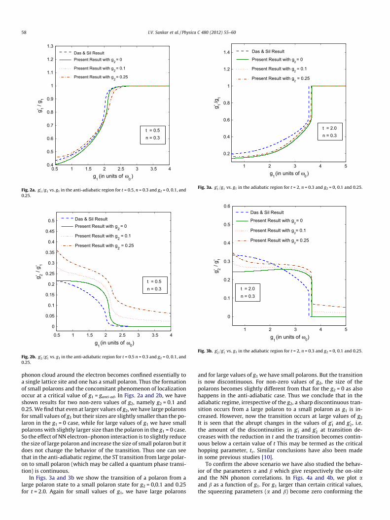
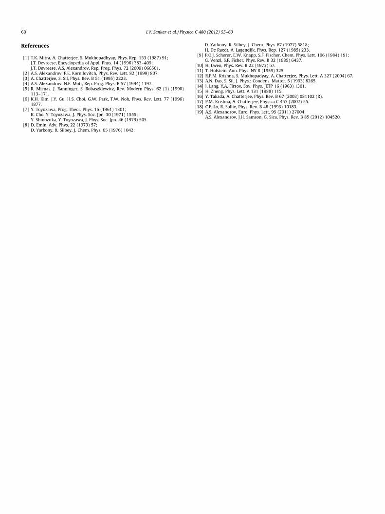
In Figs. 2a and 2b, we have shown the variations of g01=g1 (Fig. 2a)and g02=g01 (Fig. 2b) with on-site electron–phonon strength g1 for theelectron concentration n = 0.3 and for different values of NN elec-tron–phonon strength (g2 = 0,0.1,0.25) for the anti-adiabatic case.One can find out from the figures that for small values ofg1; g

01 < g1, but g02 > g2 which implies that in this region the phonon

cloud associated with the polaron is thin but is spread over manylattice sites and thus one has a large polaron. As g1 increases, g01 alsoincreases and eventually becomes equal to g1, but g02 decreases sub-stantially so much so that g02 becomes smaller than g2. Thus the

1 2 3 4 5

0.2

0.4

0.6

0.8

1

1.2

1.4

g1 (in units of ω0 )

g’ 1/g

1

Das & Sil Result

Present Result with g2 = 0

Present Result with g2 = 0.1

Present Result with g2 = 0.25

t = 2.0n = 0.3

Fig. 3a. g01=g1 vs. g1 in the adiabatic region for t = 2, n = 0.3 and g2 = 0, 0.1 and 0.25.

1 2 3 4 5

0

0.1

0.2

0.3

0.4

0.5

0.6

g1 (in units of ω0 )

g’ 2 / g’ 1

Das & Sil Result

Present Result with g2 = 0

Present Result with g2 = 0.1

Present Result with g2 = 0.25

t = 2.0n = 0.3

Fig. 3b. g02=g01 vs. g1 in the adiabatic region for t = 2, n = 0.3 and g2 = 0, 0.1 and 0.25.

0.5 1 1.5 2 2.5 3 3.5 40.4

0.5

0.6

0.7

0.8

0.9

1

1.1

1.2

1.3

g1 (in units of ω

0 )

g’ 1 / g 1

Das & Sil ResultPresent Result with g2 = 0

Present Result with g2 = 0.1

Present Result with g2 = 0.25

t = 0.5n = 0.3

Fig. 2a. g01=g1 vs. g1 in the anti-adiabatic region for t = 0.5, n = 0.3 and g2 = 0, 0.1, and0.25.

0.5 1 1.5 2 2.5 3 3.5 4

0

0.05

0.1

0.15

0.2

0.25

0.3

0.35

0.4

0.45

0.5

g1 (in units of ω0 )

g’ 2 / g’ 1

Das & Sil ResultPresent Result with g

2 = 0

Present Result with g2 = 0.1

Present Result with g2 = 0.25

t = 0.5n = 0.3

Fig. 2b. g02=g01 vs. g1 in the anti-adiabatic region for t = 0.5 n = 0.3 and g2 = 0, 0.1, and0.25.

58 I.V. Sankar et al. / Physica C 480 (2012) 55–60

phonon cloud around the electron becomes confined essentially toa single lattice site and one has a small polaron. Thus the formationof small polarons and the concomitant phenomenon of localizationoccur at a critical value of g1 = ganti-ad. In Figs. 2a and 2b, we haveshown results for two non-zero values of g2, namely g2 = 0.1 and0.25. We find that even at larger values of g2, we have large polaronsfor small values of g1 but their sizes are slightly smaller than the po-laron in the g1 = 0 case, while for large values of g1 we have smallpolarons with slightly larger size than the polaron in the g1 = 0 case.So the effect of NN electron–phonon interaction is to slightly reducethe size of large polaron and increase the size of small polaron but itdoes not change the behavior of the transition. Thus one can seethat in the anti-adiabatic regime, the ST transition from large polar-on to small polaron (which may be called a quantum phase transi-tion) is continuous.

In Figs. 3a and 3b we show the transition of a polaron from alarge polaron state to a small polaron state for g2 = 0,0.1 and 0.25for t = 2.0. Again for small values of g1, we have large polarons

and for large values of g1 we have small polarons. But the transitionis now discontinuous. For non-zero values of g2, the size of thepolarons becomes slightly different from that for the g2 = 0 as alsohappens in the anti-adiabatic case. Thus we conclude that in theadiabatic regime, irrespective of the g2, a sharp discontinuous tran-sition occurs from a large polaron to a small polaron as g1 is in-creased. However, now the transition occurs at large values of g2

It is seen that the abrupt changes in the values of g01 and g02, i.e.the amount of the discontinuities in g01 and g02 at transition de-creases with the reduction in t and the transition becomes contin-uous below a certain value of t This may be termed as the criticalhopping parameter, tc. Similar conclusions have also been madein some previous studies [10].

To confirm the above scenario we have also studied the behav-ior of the parameters a and b which give respectively the on-siteand the NN phonon correlations. In Figs. 4a and 4b, we plot aand b as a function of g1. For g1 larger than certain critical values,the squeezing parameters (a and b) become zero conforming the

0.5 1 1.5 2 2.5 3 3.5 4 4.5

0

0.5

1

1.5

2

2.5

g1 (in units of ω

0 )

t e (i

n un

its o

f ω0 )

Das & Sil Result Present Result with g

2 = 0

Present Result with g2 = 0.25

t = 2

t = 0.5

Fig. 5. Variation of te with g1 for n = 0.3, t = 0.5 and 2, and g2 = 0 and 0.25. Theresults of Das and Sil [13] are represented by dashed lines.

0.5 1 1.5 2 2.5 3 3.5 4 4.5−0.02

−0.01

0

0.01

0.02

0.03

0.04

0.05

0.06

0.07

g1 (in units of ω0 )

β

Das & Sil Result (β = 0) Present Result with g2 = 0

Present Result with g2 = 0.25

t = 0.5

t = 2

Fig. 4b. b vs. g1 for n = 0.3, t = 0.5 and 2 and g2 = 0 and 0.25.

0.5 1 1.5 2 2.5 3 3.5 4 4.5−0.05

0

0.05

0.1

0.15

0.2

0.25

0.3

0.35

g1 (in units of ω0 )

α

t = 2

t = 0.5

Das & Sil Result Present Result with g2 = 0 Present Result with g2 = 0.25

Fig. 4a. a vs. g1 for n = 0.3, t = 0.5 and 2 and g2 = 0 and 0.25.

I.V. Sankar et al. / Physica C 480 (2012) 55–60 59

existence of localized (small) polarons in both the anti-adiabaticand adiabatic cases. One can observe that the optimum values ofa increase with increasing g1, reach their maxima and then startdecreasing and finally go to zero continuously as g1 approaches acritical value ganti-ad for t = 0.5, while for t = 2, a drops to zerodiscontinuously from its maximum as g1 approaches the criticalvalue gad. The behavior of b is however slightly more dramatic inthe anti-adiabatic case. As g1 increases, b also increases andreaches a maximum, but on further increase in g1, b decreases toa negative value and as g1 increases further, it goes to zero contin-uously at g1 = ganti-ad. The behavior of b in the adiabatic case is sim-ple. As g1 increases, b increases monotonically to a maximum andthen decreases on further increase in g1 and finally drops to zero dis-continuously at g1 = gad. As we have already pointed out,ganti-ad < gad. It is clear from the above argument that the phononcorrelation effects are most important in the intermediate-couplinglimit and are essentially unimportant in strong-coupling limit.

To reconfirm the nature of the ST transition, we finally study thevariation of the effective hopping integral te which is proportional

to the polaron band width and thus gives a measure of the polaronmass which is a physical quantity. Fig. 5 shows that te is a decreas-ing function of g1 which is however understandable because of theband narrowing effect associated with the polaron formation. Ourresults suggest that te decreases as g1 increases and finally becomezero continuously for t = 0.5 but, for t = 2 our results predict a con-tinuous decrease in te only until g1 attains a critical value of 3.7 atwhich however te undergoes a discontinuous drop indicating asharp ST transition.

5. Conclusions

We have studied the nature of ST transition in an extended HHmodel in two dimensions using a variational method. We haveemployed a modified LF and an electron-number-independentcoherent state transformations and then an on-site and an NNtwo-phonon correlated squeezing transformations followed by an-other coherent state transformation to obtain an effective ex-tended Hubbard model which we have solved by the mean-fieldHartree–Fock approximation. Our results show that the ST transi-tion is continuous in the anti-adiabatic regime and discontinuousfor the adiabatic case. It has been pointed out by Das and Sil thatthe discontinuity in the ST transition in the adiabatic case could bedue to insufficient number of variational parameters used in theirwave function. Since in our calculation we have considered quitean accurate wave function with a good number of parameters,the discontinuity at the ST transition, if at all is an artifact, couldbe arising due to mean-field approximation. Therefore a bettermethod to deal with the effective Hubbard model is certainlycalled for. Such an investigation is under progress and results willbe published in due course.

We would like to mention at the end that our method involvesvariational canonical transformations followed by averaging overphonon vacuum and thus neglects second-order contributions tothe polaron self-energy and the residual polaron–polaron interac-tions. These contributions are particularly large in the adiabatic re-gime and could be important from the point of view of origin ofhigh-temperature superconductivity in cuprates (which are highlypolarizable) as shown recently by Alexandrov [19]. The residualpolaron–polaron interaction may also produce super-light mobilebipolarons which may be ideal candidates for high temperaturesuperconductivity.

60 I.V. Sankar et al. / Physica C 480 (2012) 55–60

References

[1] T.K. Mitra, A. Chatterjee, S. Mukhopadhyay, Phys. Rep. 153 (1987) 91;J.T. Devreese, Encyclopedia of Appl. Phys. 14 (1996) 383–409;J.T. Devreese, A.S. Alexandrov, Rep. Prog. Phys. 72 (2009) 066501.

[2] A.S. Alexandrov, P.E. Kornilovitch, Phys. Rev. Lett. 82 (1999) 807.[3] A. Chatterjee, S. Sil, Phys. Rev. B 51 (1995) 2223.[4] A.S. Alexandrov, N.F. Mott, Rep. Prog. Phys. B 57 (1994) 1197.[5] R. Micnas, J. Ranninger, S. Robaszkiewicz, Rev. Modern Phys. 62 (1) (1990)

113–171.[6] K.H. Kim, J.Y. Gu, H.S. Choi, G.W. Park, T.W. Noh, Phys. Rev. Lett. 77 (1996)

1877.[7] Y. Toyozawa, Prog. Theor. Phys. 16 (1961) 1301;

K. Cho, Y. Toyozawa, J. Phys. Soc. Jpn. 30 (1971) 1555;Y. Shinozuka, Y. Toyozawa, J. Phys. Soc. Jpn. 46 (1979) 505.

[8] D. Emin, Adv. Phys. 22 (1973) 57;D. Yarkony, R. Silbey, J. Chem. Phys. 65 (1976) 1042;

D. Yarkony, R. Silbey, J. Chem. Phys. 67 (1977) 5818;H. De Raedt, A. Lagendijk, Phys. Rep. 127 (1985) 233.

[9] P.O.J. Scherer, E.W. Knapp, S.F. Fischer, Chem. Phys. Lett. 106 (1984) 191;G. Venzl, S.F. Fisher, Phys. Rev. B 32 (1985) 6437.

[10] H. Lwen, Phys. Rev. B 22 (1973) 57.[11] T. Holstein, Ann. Phys. NY 8 (1959) 325.[12] R.P.M. Krishna, S. Mukhopadyay, A. Chatterjee, Phys. Lett. A 327 (2004) 67.[13] A.N. Das, S. Sil, J. Phys.: Condens. Matter. 5 (1993) 8265.[14] I. Lang, Y.A. Firsov, Sov. Phys. JETP 16 (1963) 1301.[15] H. Zheng, Phys. Lett. A 131 (1988) 115.[16] Y. Takada, A. Chatterjee, Phys. Rev. B 67 (2003) 081102 (R).[17] P.M. Krishna, A. Chatterjee, Physica C 457 (2007) 55.[18] C.F. Lo, R. Sollie, Phys. Rev. B 48 (1993) 10183.[19] A.S. Alexandrov, Euro. Phys. Lett. 95 (2011) 27004;

A.S. Alexandrov, J.H. Samson, G. Sica, Phys. Rev. B 85 (2012) 104520.