1

Locate Your Nearest Exit: Mass Layoffs and Local Labor Market Response

Andrew Foote

afoote@ucdavis.edu

Michel Grosz mgrosz@ucdavis.edu

Ann Stevens annstevens@ucdavis.edu

Department of Economics

University of California, Davis

April 2015

Abstract

Large shocks to local labor markets cause lasting changes to communities and their residents. In this paper, we examine four main components through which individuals exit the local labor force following large labor demand shocks: in-migration, out-migration, retirement, and enrollment in disability insurance. First, we document the magnitude of the response through these channels after a mass layoff event showing that, primarily through migration, they account for roughly three-fourths of labor force reductions. Additionally, we explore the residual difference between these channels and the labor force change, which we argue is due to labor force non-participation by individuals. We find that this residual is larger in the period following the Great Recession, which highlights the growing importance of non-participation as a response to labor demand shocks. Finally, we find evidence that mass layoff events cause individuals to undertake long-distance migration rather than migration to adjacent counties.

*We are grateful to Ben Hansen for generously sharing his mass layoffs data and expertise with

us. We also thank seminar participants at Texas A&M, UC Davis, UCSD and the 2014 Western

Economic Association meeting.

2

1 Introduction

Over the course of the Great Recession, rates of job loss in the United States reached record

highs. As the recovery continues, understanding the nature and speed of labor market adjustment is

more important than ever. At the national level, much of the public attention and media coverage

has been on overall levels of job creation and economic activity. Variation across local areas in the

depth of the downturn points to a need to focus the policy discussion on re-allocating workers to

jobs. Well-known work by Blanchard and Katz (1992) originally emphasized the importance of

labor mobility in this adjustment process: local unemployment rates are primarily driven by

workers moving to areas where there are more jobs, as opposed to local job creation. During the

Great Recession, reports of significantly reduced mobility (Frey 2009) have added to concerns that

housing market factors and low mobility may prolong recovery time.

In this paper, we examine the relationship between negative local labor market shocks—many

of which occurred during the recent recession—and labor force changes. Specifically, we ask

whether, and to what extent, internal migration and other exits from the local labor force follow

negative shocks and facilitate adjustments in an area’s labor supply. We measure changes in county

population, labor force, migration, retirement and disability insurance enrollment that occur

following large layoff events.

There are various benefits to use mass layoffs as the measure of local labor demand shocks.

First, we avoid some of the endogeneity of local unemployment rates with respect to changes in

labor supply and migration patterns. Second, the mass layoffs afford us the opportunity to analyze

responses to local labor demand shocks that are discrete and do not occur over the course of several

years. Relatedly, since mass layoffs are defined as the permanent release of at least 50 workers from

a single establishment, they represent a permanent and concentrated shock to local labor demand.

We first measure the net change in the size of the local labor force in response to a mass layoff.

There are a variety of causes for these labor force changes, we focus on four main channels of labor

market exit—in-migration, out-migration, enrollment disability insurance, and retirement—and we

estimate the relative importance of these channels as a exits from the labor force. These four exit

3

channels jointly account for most of the observed net changes in labor force, and we argue that the

residual is mainly composed of exits due to labor force non-participation. We show that while

migration is the predominant channel of labor force exit, non-participation grew in importance

during the Great Recession.

This paper makes several contributions to the literature. First, we unify and update

observations about labor market adjustments following local labor market exit, and compare the

relative importance of these channels. Second, we directly measure the role of migration as an

adjustment mechanism in the aftermath of significant mass layoffs affecting an area’s residents.

While the relationship between unemployment rates and migration has been studied extensively,

we are the first to directly and systematically link mass layoff events to mobility into and out of local

areas. Finally, we document the rising importance of non-participation following local labor demand

shocks in recent years, and discuss potential reasons for that change.

The remainder of this paper is organized as follows. First, in Section 2 we discuss the prior

literature on labor demand shocks and labor market exit. In Section 3, we discuss the data sets that

we use and present summary statistics, while in Section 4 we present our decomposition of net

labor force changes, and discuss our estimation strategy. In Section 5, we present our reduced form

estimates, and discuss our estimates of the non-participation channel. Finally, Section 6 concludes.

2 Literature Review

There is a substantial literature on the effect of labor demand shocks on migration. Blanchard

and Katz (1992) show that after a negative employment shock, employment in a local labor market

falls and then recovers somewhat, but never returns to its original level. They conclude that most of

this effect is due to migration. Here, we update and extend their approach in order to more directly

document the size of these flows out of labor markets following a negative labor demand shock.

Bound and Holzer (2000) measure the responsiveness of specific populations between the 1980

and 1990 Censuses to labor market shocks. They show that low-skilled workers, particularly low-

skilled black workers, migrate relatively little in response to labor market shocks. We re-examine

4

this issue using mass layoffs. We also include measures of population changes by age and race

groups, which allow us to examine how labor force responses to mass layoffs affect an area’s

demographic composition.

Notowidigdo (2013) extends Bound and Holzer’s (2000) analysis and employs a similar method,

but argues that lower-skilled workers are less likely to migrate because they bear a smaller

incidence of local labor demand shocks. He shows that following adverse labor demand shocks,

public assistance program spending increases and housing costs decline, which both

disproportionately impact low-skilled workers and make them less likely to migrate. He also notes

that some of the decline in local employment is due to a decline in labor force participation, and

cannot be entirely attributed to out-migration. Our work directly measures these channels, in order

to assess the importance of non-participation.

Saks and Wozniak (2011) show that migration is pro-cyclical at the national level; in times of

low national unemployment, the benefits to moving are higher, inducing more people to migrate for

job-related reasons. Additionally, when controlling for national-level labor demand, they find that

state-level labor demand is still a significant determinant of migration.

In this paper, we examine shocks that are more acute and localized than state-level

unemployment changes, by measuring mass layoff events at the county level. In addition to

migration, we explore how other channels of labor force exit are related to aggregate economic

cycles. The first of these is Social Security Disability Insurance enrollment (hereafter DI), whose role

as an alternative to job search in economic downturns has been documented in various contexts

(Black et al. 2002, Burkhauser et al. 2004, Autor and Duggan 2003). The second additional channel

of labor market exit is retirement, which we observe in takeup of Social Security retirement

benefits. Workers displaced from jobs late in their careers have substantially lower employment

rates than those who are not displaced, which suggests that poor re-employment prospects after

mass layoffs cause many workers to opt for early retirement (Chan and Stevens, 1999, 2001;

Stevens and Chan, 1999). Others suggest that different aspects of the recent economic downturn–

the housing market crash, the stock market collapse, and rising unemployment–imply different

5

incentives to either hasten or delay retirement (Coile and Levine, 2011; Bosworth and Burtless,

2010 and Goda et al. 2012).

Workers, especially those who have been laid off, may also exit the labor force without

migrating or substituting their former income with participation in government programs.

Especially in hard economic times, unemployed workers may become discouraged and stop looking

for work (Erceg and Levin 2013). In the Great Recession, the labor market saw a surge in exits due

to discouraged workers, only half of whom eventually reentered the labor market (Ravikumar and

Shao 2014, Kwok et al. 2010). Workers are also more likely to become discouraged or take longer to

reenter the labor force if part of a couple, since the other member of the couple may increase job

search or enter the labor market, a phenomenon dubbed the added worker effect (Lundberg 1985,

Mattingley and Smith 2010). In the Great Recession, as in other economic downturns, labor force

participation among teenagers also decreased, as more pursued education or simply did not work

or look for jobs (Kwok et al 2010).

Autor, Dorn and Hanson (2013) use differential exposure to import competition from China to

identify areas with adverse labor demand shocks. They find that these shocks lowered labor force

participation and increased unemployment, while also increasing transfer payments. While we use a

different labor market shock, we come to similar conclusions, showing that non-participation is a

key channel of adjustment following a labor demand shock. In contrast, we find effects on the

mobility of individuals; however, our results may differ because they use labor demand shocks on

lower-skilled workers, who are not as mobile.

3 Data

We compile various datasets to construct a panel of counties spanning the years 1996-2013. Our

identification strategy relies on variation in county-level labor demand shocks, as measured by large

mass layoff events. To measure the size of these shocks, we calculate the share of the county labor

force in a given year that that was displaced due to a mass layoff. Between 1996 and 2013, the

Bureau of Labor Statistics (BLS) compiled monthly reports on layoffs by observing the initial claims

6

for unemployment insurance filed by workers. The BLS identified a mass layoff event when more

than 50 workers file claims against a single establishment within any five-week period. For these

events, the BLS contacted the establishment to determine whether these workers experienced a

layoff of at least 31 days. We use data on these mass layoff events at the county level for 1996-2013,

including the number of workers directly affected.1 Our data are organized by the affected workers’

county of residence, so that we measure the number of workers living in a given county who were

part of a mass layoff at their past establishment (which could be located in a different county). To

normalize the magnitude of these layoffs we use annual data on the size of the county labor force,

compiled by the Local Area Unemployment Statistics program of the BLS.

Our main outcomes of interest are in-migration flows, out-migration flows, net changes in DI

caseload, and net changes in the number of retirees. We use information on migration from the

Internal Revenue Service (IRS) Statistics of Income files, which calculate inflows and outflows based

on address changes of individual tax filers. As in other research, we use the number of tax returns in

a county as an approximation for the number of households, and the number of exemptions for the

number of individuals (Molloy, Smith and Wozniak, 2011). We use these data for 1996-2012 to

construct measures of the number of individuals moving into and out of a particular county.

While these data are helpful in studying internal migration, they have a few limitations. First

and foremost, individuals who do not file taxes (most often the poor and the elderly) do not appear

in the data, nor do their households. Moreover, the data only include filers who complete their tax

returns at most five months following the April 15 deadline, which excludes some late filers. The

data are also limited in their ability to identify changes in filing status; for example, for a married

couple that subsequently divorces and files two separate returns, only the migration behavior of the

individual who was the primary taxpayer in the initial joint return will be recorded.2

To calculate the number of individuals at the county level enrolled in DI and retirement, we use

data from the Social Security Administration’s Old Age, Survivors and Disability Insurance (OASDI)

1 In March 2013, in order to abide by the sequestration imposed by the Balanced Budget and Emergency

Deficit Control Act, the BLS eliminated the Mass Layoffs Statistics Program.

2 A more extended discussion of these data, as well as their strengths and limitations, is in Gross (1999).

7

program from 1999 to 2012. While individuals can claim their retirement benefits almost

immediately upon making the decision to retire, DI enrollment occurs long after an applicant files

the initial claim. DI rules require that applicants have stopped working for five months before

applying. Applications take many months to be accepted, and applicants can appeal decisions,

extending the process. The process lasts around nine months for applications accepted on the first

claim (Kreider, 1998), but often lasts more than a year when applicants appeal (Autor et al 2011).3

We express our four outcome variables—in-migration, out-migration, DI enrollment and

retirement—as rates, which can be compared to the flows of newly displaced workers from mass

layoffs. We define in-migration and out-migration rates as the number of in- or out-migrants to or

from a county in a particular year as a share of that county’s population that year. For both DI

enrollment and retirement, we also divide the net change in new cases by the county’s population

the previous year, in order to not include the change in the labor force during the same year as the

mass layoff.

We supplement these main sources of data with additional information on county demographics

and median income. We use county level information on the age, gender, and racial composition of

county populations as reported in the Surveillance, Epidemiology, and End Results (SEER) program

of the National Cancer Institute, which includes annual data from 1969-2012, as well as county-level

median income from the Bureau of Economic Analysis (BEA).

4 Methods

Our goal is to measure the effect of mass layoffs on changes in the labor force, and to quantify

the channels of labor market exit and their relative importance. In this section, we describe the

outcomes of interest, which are the various types of labor force exits, and how they relate to each

3 Because of this attribute of the program, other studies that examine DI as a response to labor market shocks

(eg. Autor and Duggan, 2003, Black et al., 2002) tend to focus on applications as opposed to acceptances. While application behavior is certainly the most immediate response, the purpose of this paper is to document labor force exits following economic downturns. If disability insurance applicants who are rejected decide to move, or to find a new job, using application data would lead us to double count these workers. We are currently in the process of obtaining application data from the Social Security Administration.

8

other. After this description, we explain the rationale for using mass layoffs as a measure of labor

demand shocks. We discuss the limitations of using the unemployment rate by showing biased

results when instrumenting for unemployment rate with the share of the labor force involved in a

mass layoff. Second, we illustrate how mass layoffs act as well-defined shocks that are plausibly

exogenous with respect to pre-existing trends.

4.1 Decomposing Changes in the Labor Force

Consider the following decomposition of a net labor force change from one year to the next:

𝐿𝐹𝑐𝑡 − 𝐿𝐹𝑐,𝑡−1 = (𝑖𝑛𝑚𝑖𝑔𝑟𝑎𝑡𝑖𝑜𝑛𝑐𝑡 − 𝑜𝑢𝑡𝑚𝑖𝑔𝑟𝑎𝑡𝑖𝑜𝑛𝑐𝑡) − 𝐷𝐼 𝑒𝑛𝑟𝑜𝑙𝑙𝑐𝑡 − 𝑟𝑒𝑡𝑖𝑟𝑒𝑚𝑒𝑛𝑡𝑐𝑡 + 𝜑𝑐𝑡 (1)

The term 𝐿𝐹𝑐𝑡 is a county c’s labor force in year t. The above equation shows that changes in the

labor force can arise from five different channels. The first two terms on the right-hand side of

equation (1) comprise the net migration of workers: in-migration minus out-migration. Any

individuals that enroll in DI or retire also change the size of the labor force. The residual, 𝜑𝑐𝑡,

includes all other flows into and out of the labor force not captured by migration, DI, or retirement.

Foremost among these other exits from the labor force include individuals aging, workers dying, and

new full-time students. Another important component of 𝜑𝑐𝑡 is individuals of working age not

participating in any of these explicit labor force exit channels.

In order to compare the effect of layoff events across labor markets of different sizes, we

normalize the magnitude of these changes and express them as shares. Specifically, we divide both

sides of equation (1) above by the size of the population in previous period:

𝐿𝐹𝑐𝑡 − 𝐿𝐹𝑐,𝑡−1

𝑝𝑜𝑝𝑛𝑐,𝑡−1= (

𝑖𝑛𝑚𝑖𝑔𝑟𝑎𝑡𝑖𝑜𝑛𝑐𝑡

𝑝𝑜𝑝𝑛𝑐,𝑡−1−

𝑜𝑢𝑡𝑚𝑖𝑔𝑟𝑎𝑡𝑖𝑜𝑛𝑐𝑡

𝑝𝑜𝑝𝑛𝑐,𝑡−1) −

𝐷𝐼 𝑒𝑛𝑟𝑜𝑙𝑙𝑐𝑡

𝑝𝑜𝑝𝑛𝑐,𝑡−1−

𝑟𝑒𝑡𝑖𝑟𝑒𝑚𝑒𝑛𝑡𝑐𝑡

𝑝𝑜𝑝𝑛𝑐,𝑡−1+ �̂�𝑐𝑡 (2)

This equation above describes the relationship between our five outcome variables of interest. We

estimate the effect of mass layoffs on the components of the right-hand side of equation (2), as well

as on the net change in labor force (i.e. the left hand side of equation (2)). The residual �̂�𝑐𝑡 is just

rescaled from the first equation. We normalize in this way in order to avoid scale-effect bias, as

described in Peri and Sparber (2011).

9

Note that in equation (2) above, the in-migration and out-migration specifically refer to labor

force participants. While the migration data we use do not separate out workers from non-workers,

if we assume that labor force participants to non-participants migrate at the same rate, then those

two terms do not have to be rescaled.

4.2 Concerns with County Unemployment Rates and Mass Layoff Counts as an Alternative

Understanding the relationship between local labor market shocks and labor force exits

presents several challenges. First, a typical approach involves relating local area unemployment

rates to local population changes or migration rates.4 However, the unemployment rate is itself a

function of current and past migration decisions, making causal inference difficult and

interpretation of descriptive relationships challenging. Second, analyses are typically done at the

state level, which may be too broad to capture a single labor market. One the other hand, local

unemployment measures for smaller geographic areas raise serious measurement error concerns.

We begin our analysis by measuring the effect of the unemployment rate on labor force exit,

knowing the limitations of such an approach. In our context, with local labor market changes

measured at the county level, we estimate the following equation:

𝑦𝑐𝑡 = 𝛼 + 𝛽𝑈𝑅𝐴𝑇𝐸𝑐𝑡 + 𝛿𝑡 + 𝛾𝑐 + 𝜂𝑐 ∗ 𝑡 + 𝜖𝑐𝑡 (4)

where yct is a particular type of labor market exit measured at the county level, and URATEct is the

unemployment rate in the county. We also include time fixed effects δt and county fixed effects γc,, as

well as county-specific time trends ηc*t.

Using the unemployment rate as above introduces three problems into the estimation. First,

the unemployment rate is endogenous since it captures labor supply changes in addition to labor

demand changes (Bartik 1996). Additionally, changes in the labor force in—the denominator of the

unemployment rate—are clearly endogenous to migration rates in and out of a local area. Finally, for

smaller geographic units the unemployment rate published by the BLS is measured with error (see

Bartik, 1996; Hoynes, 2000; Lindo 2015).

4 For examples of this, see Greenwood (1997) and Davies, Greenwood and Li (2001). Additionally, Wozniak (2010) uses both unemployment rates and Bartik instruments, while Saks and Wozniak (2011) instrument for unemployment rates with Bartik-type instruments and oil shocks; these instruments are discussed below.

10

For these reasons, researchers often rely on instruments for the unemployment rate. The

ideal instrument would address both the endogeneity concerns and concerns with measurement

error in the unemployment rate. One such instrument is the shift-share or Bartik instrument (Bartik,

1991) that utilizes pre-existing, area-specific industry structure and changes in industry outcomes

at the national level. Such an approach been used successfully at the state and MSA level (Saks and

Wozniak (2011); Bound and Holzer (2000)). However, using a Bartik instrument may be difficult at

the county-level due to small samples for measuring county-level industry shares. Additionally, the

Bartik instrument does not provide intuition on the relative size of the shock for a county, compared

to the size of the labor force.

As an alternative, in this study, we use measures of mass layoffs at the county level as our

indicator of local labor demand shocks. In our main results, we move to using mass layoff indicators

in a reduced-form setting; this has a direct and substantively interesting interpretation of the effect

of a major layoff event on a local area labor force. Mass layoffs are a good alternative to the

unemployment rate because they resolve the two problems that arise when using the county

unemployment rate. First, they clearly measure a change in labor demand, and thus are not

hampered by endogenous labor supply responses, a claim for which we provide more evidence in

the next section. While migration can mechanically reduce the unemployment rate over time,

migration does not directly generate mass layoffs. Second, measurement error in the mass layoffs

data is most likely uncorrelated with the measurement error in the county unemployment rate. The

main source of measurement error in the mass layoffs data comes from establishments planning a

certain number of layoffs and then changing these plans, and is not due a direct result of small

sample sizes, since these represent a census of all layoffs of greater than 50 workers.

Mass layoffs are also of independent interest as an observable indicator of a shock to local

labor markets that may concern policymakers. Focusing on mass layoffs allows us to directly

address the question of how a series of mass layoffs may permanently change the size and

composition of the local labor force. Similarly, we can examine how the number of lost jobs

translates into individuals leaving a local area.

11

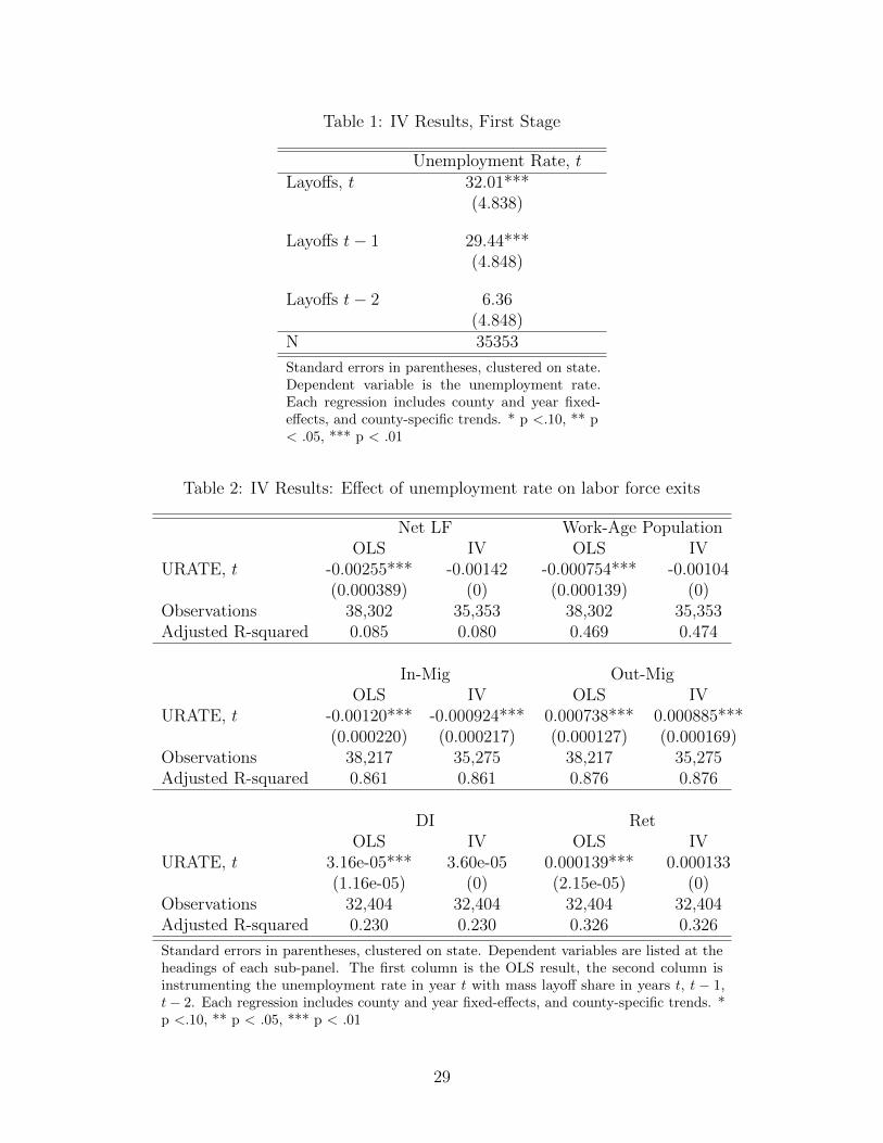
To establish that mass layoffs are strongly correlated with the unemployment rate, we begin

by regressing the unemployment rate on mass layoffs; we include the contemporaneous mass layoff

share and two lags. Table 1 summarizes the first-stage relationship between the county

unemployment rate and mass layoffs (as a fraction of the county’s labor force). This approach also

conditions on county fixed effects, year fixed effects, and county-specific trends. The F-statistic on

the mass layoffs is 30.68, and the results clearly show that mass layoffs are strongly correlated with

the unemployment rate.

We next estimate both OLS and instrumental variables versions of equation 4. As in Saks and

Wozniak (2011), we do not include lags because the unemployment rate is not a flow variable. We

instrument the unemployment rate with a contemporaneous mass layoff rate as well as two lags.5

Our results are in Table 2. Starting with the OLS results, we see small negative effects of the

unemployment on rates of in-migration. A one percentage point increase in the unemployment rate

leads to a 0.1 percentage point decrease in the in-migration rate, and the IV results are statistically

indistinguishable.

For out-migration, both the OLS estimates suggest that a one percentage point increase in

the unemployment rate increases the out-migration rate by about 0.07 percentage points. The IV

results suggest a larger initial effect of the unemployment rate on out-migration, which is consistent

with the unemployment rate being endogenous as well as with measurement error pushing the OLS

estimate towards zero.

When we look at the effects of unemployment on flows into disability insurance and

retirement, we find, as might be expected, smaller responses. This expectation is based on the fact

that only a subset of workers in a local area will have an underlying medical condition or be in an

age range that is consistent with entering disability insurance or retirement. Nevertheless, our

results do show that higher unemployment is associated with small increases in the share of a

county’s labor force that is retired or using disability insurance, echoing much earlier work. We are

the first, to our knowledge, to use mass layoffs to illustrate this connection between labor market

5 In results not shown, we included different specifications of the number of lags of both the endogenous regressor and the instrument. All the results were similar as the ones shown.

12

shocks, disability insurance and retirement. In the remainder of the paper, we focus on the reduced

form relationship between mass layoffs and labor force exits.

4.3 Mass Layoffs and Labor Force Exits

Table 3 (Panel A) shows summary statistics for layoff variables in the full study period, as well as

before and after the start of the Great Recession in 2007. On average, 0.7 percent of a county’s labor

force was laid off in a mass layoff event each year, which translates to an average of 379 workers.

Not surprisingly, these shares differ substantially before and after 2007. Panel B of Table 3 shows

the share of counties that experienced at least one year where the share of the labor force involved

in a mass layoff surpassed a certain threshold. Most counties (61 percent) had at least one year

where one percent of the labor force was laid off. A large number, however, also experienced an

event of higher percentages. Panel C of Table 1 shows the key variables that comprise the

decomposition of the change in labor force as a share of the population. On average, the change in

the size of the labor force as a share of the population was 0.3 percent.

To motivate the analysis, we illustrate the relationships between labor force exits and layoffs

using an event study approach. We focus first on counties that experienced large, discrete labor

demand shocks, which allows us to examine county trends prior to a major layoff. For these

counties, the event study analyses provide suggestive evidence that the large layoff events were

unlikely to have been precipitated by long-term labor market decline.

We limit the data to the subset of counties in our sample that experience a large layoff

event—of two, three, or four percent of the labor force—once between 2001 and 2007. We further

limit the sample to counties for which this one-time event occurred before 2007: layoff rates

increased dramatically during the Great Recession making it more difficult to isolate counties with

only a single large layoff event after 2007. In this limited sample of 118 counties, these large and

isolated layoff events were the most likely to have been unanticipated to local workers and

unrelated to local economic trends.

We estimate the following model:

13

𝑦𝑐𝑡 = 𝛼 + ∑ 𝛽𝑖1(𝑡 − 𝑇𝑐 = 𝑖)

6

𝑖=−6𝑖≠−1

+ 𝛿𝑡 + 𝛾𝑐 + 𝜖𝑐𝑡 (5)

The outcome variable yct is one of the following: in-migration rate, out-migration rate, new DI

enrollment, and new retirement enrollment. We include county and time fixed effects, γc and δt, to

control for fixed differences between counties and a non-parametric national time trend. We define

Tc as the year the county experienced layoffs surpassing the relevant layoff threshold of two, three

or four percent. The indicator 1(t − Tc = i), then, takes a value of one when the observation year is i

years from Tc. For example, if the layoff event happened in 2004, then 1(t − Tc = i) would take value

one in year 2005 for i = 1. Observations earlier than six or later than six years from the event are

captured by dummies 1(t − Tc ≤−6) and 1(t − Tc ≥ 6). We omit the dummy for i =-1, so all the

coefficients are relative to the year before the major mass layoff occurred.

The top two graphs of Figure 1 display the coefficients of our event study analyses for in- and

out-migration, as well as a 95 percent confidence interval. Appendix Figures A1 and A2 shows these

results for other lower thresholds for defining large mass layoffs. Importantly, in neither the in-

migration nor the out-migration case does there seem to be a noticeable trend in migration rates

before the mass layoff event. In-migration and out-migration seem relatively flat in the years

previous to the event. Following the event, there does appear to be an increase in out-migration

rates. Similarly, there is a noticeable dip in in-migration, which is sustained in the years following

mass layoffs.

The bottom half of Figure 1 displays the same analyses for DI and retirement. The estimates are

noisier, but the trends prior to mass layoff events do not suggest that there were upward trends in

exits to disability or retirement prior to the layoff events. Although the estimates are not statistically

significant, DI enrollment seems to increase slightly three years after the layoff event. For

retirement, the pattern is also not statistically significant but consistent with our hypotheses: two

years of increased retirement are followed by a decline in the subsequent years.

This visual analysis shows that for the counties that experienced only one major mass layoff

event in our time period, there were no pre-existing trends in labor force exit paths before the mass

14

layoff event occurred. This further motivates and provides support for our statistical approaches

below, which use mass layoffs both as an instrument for county unemployment rates, and more

directly as an indicator of local labor market shocks. In the next sections we extend the analysis to

all counties in the country—not just the ones that experienced particularly dramatic labor market

shocks—and quantify the size of these adjustment processes.

5. Effects of mass layoffs on migration and labor force exits

The previous section estimated effects on a subsample of counties. Now, we estimate the effect

for the full sample, using the following equation.

𝑦𝑐𝑡 = 𝛼 + ∑ 𝛽𝑖

2

𝑖=0

𝑙𝑎𝑦𝑜𝑓𝑓𝑐,𝑡−𝑖 + 𝛿𝑡 + 𝛾𝑐 + 𝜂𝑐 ∗ 𝑡 + 𝜖𝑐𝑡 (6)

Our key variable of interest is layoffc,t−i, which we define as the share of the labor force of county

c laid off in year t. We also include lagged values of the layoff indicators, since responses to labor

demand shocks may take time. Our outcome variable, yct, is either the net labor force change or one

of the components: out-migration rate, in-migration rate, new DI enrollment rate, and new

retirement rate, all normalized by lagged county population.

We include county fixed effects, γc, to control for systematic differences between counties in

their labor market, mobility of individuals, and the policy environment. We include year fixed

effects, δt, to control for national trends. In our preferred specification, we also include county-

specific trends, ηc ∗t, to take into account the fact that some counties have systematically growing or

declining migration rates that may be correlated with trends in labor demand and labor market

opportunities. Finally, to address the fact that mass layoffs may be correlated within a state over

time, we cluster our standard errors at the state level.

Table 4 shows our main results for out-migration and in-migration. In column 1, we include

only the contemporaneous effect of mass layoffs, while columns 2 and 3 add one and two lags,

respectively. In Column 3, the effect of mass layoffs is large and significant for both out- and in-

migration. Our estimates imply that when one percent of the county-level labor force is laid off in a

15

mass layoff event, the out-migration rate increases by about 0.06 percentage points within three

years. Additionally, for in-migration, a one percent mass layoff increase leads to a decrease in in-

migration rates by about 0.09 percentage points.6

In column 4, we include county-specific trends, which shrinks the in-migration estimates

significantly in magnitude, by about two-thirds. However, the total effect is still negative and

significant. The out-migration estimates are relatively unchanged.

In the rest of the tables we focus on the total effect—that is, the sum of the contemporaneous,

lagged, and twice-lagged coefficients displayed in Table 4. Table 5 displays our results for each

outcome, in specifications both with and without county trends. The trends only change the

estimates significantly for in-migration, and importantly our estimates for the overall change in the

labor force barely change at all. In most of the following results we thus focus on estimates that

control for county-specific trends. In column 1, we show the overall effect of layoffs on the net

change in the labor force. Specifically, a mass layoff affecting 1 percent of a county’s workers leads

to a reduction of 0.15 percentage points in the size of the labor force over the next three years. The

majority of this change is driven by increased out-migration and decreased in-migration (although

the effect on in-migration is not statistically significant).

Summing up our effects across columns, we can explain about three-fourths of the change in the

labor force with these four channels. To quantify all of the labor market exit channels, we also

calculate the implied residual, given equation 2. In the results without trends, we find that the total

effect is almost identical, and a bit larger, than the measured labor force change, with an implied

residual of 0.0152. With trends, we find a residual of -0.038, which suggests that for a 1 percent

mass layoff, the number of people that leave the labor force for other reasons increases by about

0.04 percentage points. This effect is likely due in large part to non-participation, since deaths net of

labor force entrants is likely to be small.

6 In results not shown we include additional lags to the key explanatory variable. These additional lags are small and not statistically significant providing further evidence that the timeframe of adjustment to labor market shocks is relatively quick.

16

One important question in the wake of the Great Recession is whether non-participation, which

we measure as the residual, has changed over time, suggesting changes in the role of non-

participation in the labor force. A number of recent papers have sought to investigate this, noting

that the labor force participation rate for 25-54 year olds in the Great Recession fell precipitously,

and then has not recovered even in the face of an improving economy. Erceg and Levin (2013) show

that the Great Recession contributed a large amount to the decline in labor force participation.

Charles, Kroft, and Notowidigdo (2013) argue that despite being masked by the housing boom, non-

employment has seen a secular rising trend starting in the 2000s, which only revealed itself after

the housing market crash. Here, we examine whether labor force withdrawal following a negative

demand shock in the form of mass layoffs follow this pattern as well.

To see how non-participation has changed during the Great Recession, we separate the study

period in the years before and the years including and after the Great Recession: 1996-2006 and

2007-2011. Because the later period is so short, we do not include trends in these regressions;

however, we have already shown in Table 5 that trends do not largely affect our results, except for

in-migration. Table 6 shows these results, which Panel A showing the pre-Recession estimates and

panel B showing the estimates for 2007-2011.

Our results show strikingly different patterns before and during the Great Recession. First,

column 1 shows that the change in labor force in response to a 1 percent mass layoff was

substantially larger following the Great Recession. However, at the same time both in- and out-

migration are smaller in magnitudes, reflecting the secular decrease in migration over this time

period. This shows that this decline in migration rates applies specifically to the mobility response

to a negative labor market shock. Finally, the magnitudes and sign of DI and retirement are more

positive although not significant in the later period.

Overall, during the pre-recession period, our estimates imply that we over-explain the labor

force change, such that the residual— the labor force change not explained by migration or

transitions to disability or retirement --- was positive. Summing up all the effects gives us a total

17

effect of 0.1411, which is larger than the change in the labor force, and which suggests little role for

non-participation as an important part of the change in labor force participation.

For the period that includes the Great Recession, the total effect across all exit channels is -

0.0726, while the total change in the labor force is -0.1185, implying a residual of about -0.0459.

This estimate is much larger than for the pre-period, where the residual was non-existent, and

suggests that in the recent recession, non-participation became an increasingly important channel

of labor market exit.

Another way we can estimate how this effect changes pre- and post-Great Recession is by

interacting our measure of mass layoffs with a dummy for the year being after 2007. We do this in

Table 7, allowing the effect of a mass layoff to be different before and after the Great Recession. In

the table, below the coefficient estimates, we list the total effect for the time period before the

recession and after the recession.

Our results show that the non-participation channel grew much larger during the Great

Recession. The effect of a shock in the pre-recession period on net labor force was about 0.10

percentage points. Additionally, the effect of the mass layoff is large for both out-migration and in-

migration, and all the estimates taken together imply a residual of approximately 0.0264, implying

that our channels over-explain the labor force change.

The results are much different for the years after 2007. First, the labor force response to a one

percent mass layoff is about twice as large as before 2007. Second, the out-migration response is

muted, about half as large, while the point estimate on disability insurance is over twice as large,

although not significant. Taken together, our estimates suggest that migration, retirement, and

disability explain only about 40 percent of the total change in the labor force during the recession

years, with the residual (non-participation) explaining 60 percent of the net labor force change.

This is not consistent with a story of migration providing the major channel for labor market

adjustment to local shocks. One possibility is that the Great Recession was due the role of the

housing crisis, which impeded mobility. Another possibility is that during a recession, mobility

plays a more limited role in local labor market adjustment than in a non-recessionary period(Saks

18

and Wozniak, 2010). Results showing a limited role for migration are generally consistent with the

findings of Notowidigdo (2013), who suggests that migration is not the primary mechanism in the

adjustment of local labor markets.

5.1 Geography of labor force exits

In addition to exploring heterogeneity before and after the Great Recession, we expect there

to be geographic heterogeneity in the response to labor demand shocks. In particular, we expect that

responses in counties in more urban settings may be different because of differences in the density

of job opportunities, distance to other potential jobs in adjacent counties, or attitudes toward and

availability of public assistance. Additionally, some counties that are not near cities may be more

dependent on a single firm or industry, leading mass layoff events to have an outsized effect.7

We categorize counties by whether they were part of a metropolitan statistical area (MSA) as

defined in the 1990 Census. We use 1990 MSA definitions in order to fix these definitions before the

start of the study period. The results in Table 8 show a marked difference in the labor market

response by this distinction. Out-migration is large and significant for MSA counties, such that a one

percent mass layoff leads to an increase in 0.11 percentage points in the out-migration rate, a

response twice as large as for non-MSA counties. In both urban and rural counties, the response in

terms of disability enrollment and retirement is insignificant. Totaling the responses, the residual is

roughly 6 percent of the overall labor force change for urban counties, while it is over 20 percent for

rural counties, which suggests that non-participation is a more important labor market exit channel

in counties outside of metropolitan areas.

When looking at these effects pre- and post-Great Recession, the results are even more striking;

these results are in Table 9. Non-MSA counties saw much larger changes in labor force in the years

including the Great Recession, while the response in urban counties is relatively similar across time

periods. Additionally, while the residual in MSA counties did not change much, the residual in rural

7 For instance, the economy of rural Greenlee County, Arizona depends on one of the largest copper mines in

the world, which in 2001 and 2008 laid off a large number of workers and, thus, a substantial fraction of the

county’s labor force. Likewise, a series of lumber mill closings in northern Idaho in 2000, especially in

Benewah County, devastated the local economy, directly affecting four percent of the labor force.

19

counties grew from about 20 percent to over 60 percent. These results are suggestive that much of

the change in non-participation arose from counties outside of metropolitan areas.

Finally, in results not shown, we also estimate effects by region. We find that the Midwest

experienced the largest responses to mass layoffs in terms of labor force change, and that the

Midwest also had the largest residual (almost 75 percent of the total change in labor force). We also

find that most of these effects are concentrated in the Great Recession period.

One possibility for the different results for rural and urban counties might be that populous

counties react differently to these events than sparsely populated counties. Our estimates so far

measure the effect for an average county, and thus do not account for these differences. When we

weight the regressions by population prior to the study period, our results do not change

substantially. A more in-depth discussion of this issue of weighting is in Appendix A.

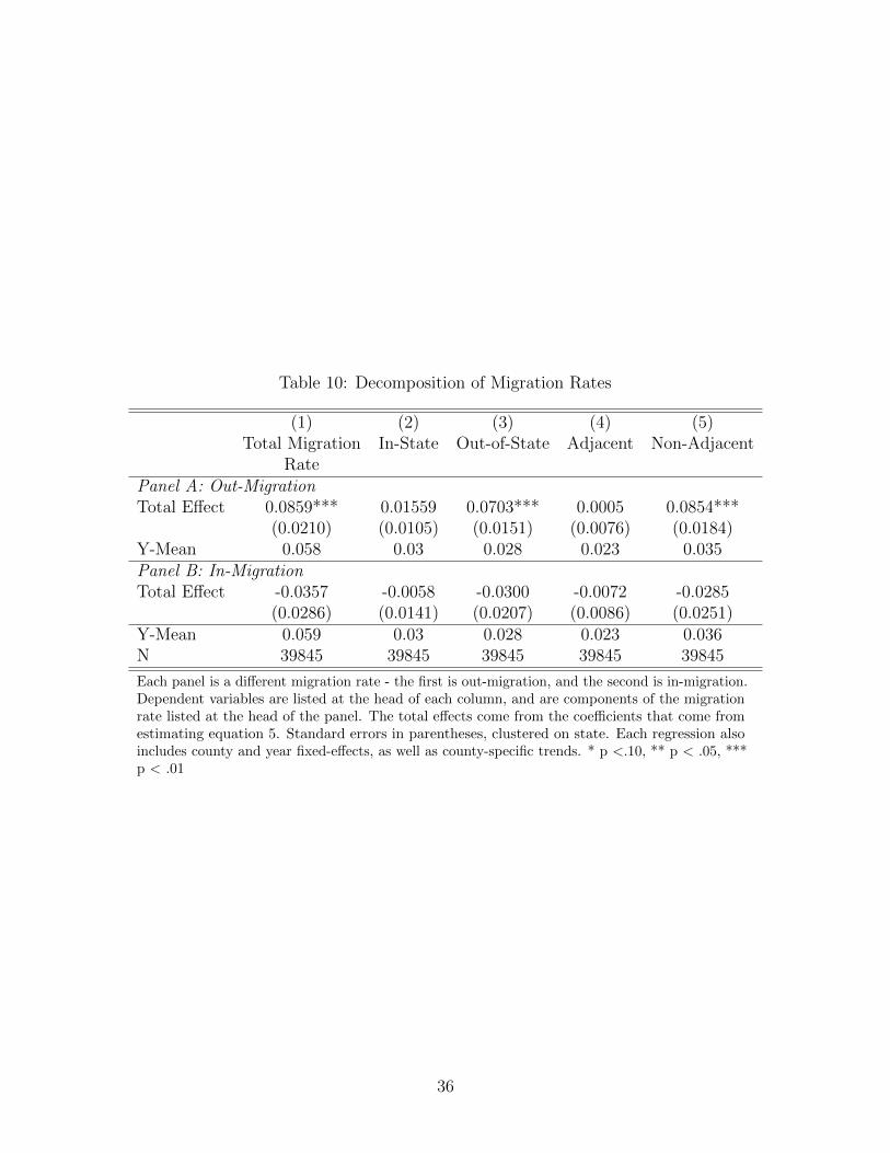
In addition to categorizing counties by their population, we also examine the distance of

movement for individuals who migrate. Fogli et al. (2012) argue that individuals displaced from

work in one county may migrate to an adjacent county, mechanically increasing its unemployment

rate. One advantage of the IRS migration dataset is that it allows us to decompose the migration

response in more detail and thus estimate the size of this effect.

We explore whether workers undertake moves across state lines or to adjacent counties. Table

10 shows the results of these decompositions. Column 1 displays the main result from Table 5,

while columns 2-5 examine the responses of the four types of migration flows. The results suggest

that the majority of people leaving the county following layoffs tend to leave the state (82 percent).

Similarly, 99 percent of moves are to non-adjacent counties. These findings suggest that individuals

seek moves to a different market, rather than simply relocating to reduce housing arrangements or

costs.

5.2 Effects Moderated by County Features

We find that the labor force exit response, as well as the relative size of different channels, varies by

whether a county is in an MSA. Following Notowidigdo (2011) we also expect these responses to be

moderated by the strength of income supports in the local safety net. Counties vary dramatically in

20

take-up and usage rates of different social programs, but these differences are often endogenous to

other local economic conditions. However, there is little cross-sectional variation in safety net

generosity. One notable exception is unemployment insurance (UI), since states are able to adjust

the replacement rate of UI benefits (Kuka 2015, Lalumia 2013). To this end, we use the UI benefit

calculator developed by Lalumia (2013) and rank states by their generosity in a year prior to our

study period, expressed as the maximum benefit level. Panel A of Table 11 shows that counties in

states with lower UI benefits see lower drops in labor force: -0.127 and -0.209 respectively.

However, out-migration in the low UI eligibility counties is not substantially lower than in other

counties (0.069 and 0.081), suggesting that the residual non-participation is higher in high UI

counties.

One of our key storylines is that the pattern of labor force adjustment changed during the

Great Recession. This recession was driven in large part by subprime lending and foreclosures. We

expect heightened subprime and predatory lending to be associated with higher rates of out-

migration for a labor market shock of equal size. Using county data from the Home Mortgage

Disclosure Act (HMDA),8 which compiles detailed information on loan originations, we ranked

counties as high or low in terms of the share of home purchase loans that were high-cost (the

di_erence between its APR and a Treasury security with the same maturity was at least 3 percent).

These are loans most likely to enter foreclosure. HMDA only began tracking this information in

2004, however, so we can only categorize counties in terms of the share of high-cost loans in the

Recession period, from 2007 onwards. Panel B of Table 11 shows these results. We find that, overall,

counties with above-median rates of high-cost loans also saw large rates of labor force exit following

mass layoffs. On the other hand, these did not necessarily have higher rates of out-migration,

8 These HMDA data files (www.metrotrends.org/natdata/hmda/hmda_download.cfm) and the

procedures for constructing them were initially developed by the Urban Institute to support

DataPlace (www.dataplace.org). The data are licensed under the Open Database License

(http:/www.metrotrends.org/natdata/ODbL.cfm).

21

suggesting instead a larger residual. This suggests that counties that were more leveraged in terms

of their risk in the impending housing market collapse also saw higher rates of labor force exit due

to non-participation, but not necessarily due to migration.

5.3 Robustness Checks Here, we briefly discuss a number of robustness checks to our basic specification. First, we re-

estimate equation 6, but also include a lead of the layoff share. If the lead is significant, it would

suggest that counties experiencing mass layoffs were generally declining in a way that was

predictable to individuals, suggesting that mass layoffs are not an unexpected labor demand shock.

As shown in Table 12, we find that most of the lead coefficients are small and statistically

insignificant. The one exception is that we estimate a statistically significant decrease in new

disability claims one year prior to mass layoffs. This is surprising, but the fact that the direction of

this effect is opposite of that expected in the aftermath of layoffs suggests that it is not driven by a

standard endogeneity story.

Additionally, we also aggregated all of our outcomes to the commuting zone level, which is a

more natural definition of a local labor market, and includes all counties in the United States. Our

estimates for those regressions are in Table 13. The total change in the labor force for a 1% mass

layoff is approximately 0.21 percentage points, which is larger than our main estimates. Overall, our

results are very similar, and the four labor market exit channels we consider can account for about

three-fourths of the change in the labor force due to mass layoffs.

The analyses so far quantify the channels of labor market exit and compared their magnitudes,

with migration being the predominant type of exit. Bound and Holzer (2000) find that different

segments of the population adjust to labor market changes to different extents. With this

heterogeneity in mind, we measure the extent to which an area’s demographic composition changes

with mass layoff events. We use the share of the population in various age and race categories as the

dependent variable in equation 6. Table 14 displays the results. While the effects are not statistically

significant, the signs of the coefficients are consistent with previous literature on migration

22

propensities, as well as our key result that migration is the predominant labor market exit. The

effects imply that following a mass layoff, the share of youth and adults early career age decrease,

suggesting that they are more likely to migrate in response to a mass layoff. On the other hand, the

positive coefficients for the share of people ages 45-59 implies that older workers are less likely to

migrate in response to a mass layoff. We also find that the share of the county that is white

decreases, while the share that is black increases, suggesting differential likelihood of migration by

race found by Bound and Holzer (2000).

6 Conclusion Researchers have long been interested in how individuals respond to adverse labor market

conditions, and how these responses serve to equilibrate the labor market. Blanchard and Katz

(1992) was the first paper to suggest that labor mobility was central to this adjustment process.

However, in the years since the Blanchard and Katz study, relatively little work has directly

examined mobility in the aftermath of specific local labor market shocks,9 while mobility rates have

been in secular decline. Additionally, the role of mobility in labor market adjustment has taken

center stage as we emerge from the Great Recession and see evidence that labor mobility seems to

be lower than at any time in recent history. This study attempts to bring these two lines of literature

together, examining mobility and other labor force adjustments to county-level mass layoff

measures.

We find that a layoff of one percent of a county’s labor force leads to a decrease in the county

labor force of 0.15 percentage points, and further find that migration accounts for a large share of

this change. In all, our four exit channels—in-migration, out-migration, retirement, and DI—account

for three-fourths of the net labor force change following a mass layoff.. Additionally, we show that

non-participation has increased in the Great Recession, and is also more predominant in rural areas.

Our finding of increased non-participation during and following the Great Recession raises a

number of important questions for further research. First, while there is anecdotal evidence of what

non-participants do with their time, to our knowledge there is no empirical work quantifying the

9 A notable exception is Zou (2015).

23

specific nature of non-participation. These former workers may be working in informal markets, or

they may be members of households with multiple earners. Additionally, it is unclear to what extent

the non-participation we observe in the Great Recession is temporary or permanent, and whether

we should expect these former workers to return to the labor force after labor market conditions

improve. As with the long-term unemployed, it is likely that the skills of these non-participating

individuals have decayed, and therefore will be less productive upon re-entering the labor force.

Second, our results on non-participation do not speak to the more aggregate effects of non-

participation on the aggregate labor market. While some researchers have tried to address this

issue broadly (Smith, 2014), much more research needs to be done on the margin of non-

participation. In particular, many job search models do not consider non-participation as a separate

state from unemployment. However, this paper shows that non-participation is an important

contributor to the adjustment process following an adverse labor demand shock.

Finally, another important question that follows from our paper is the extent to which the

effects we find may vary by the industrial composition of a local area and of the layoffs themselves.

Laid off workers may in some areas readily find work in a similar industry, while in other areas

similar jobs may not be available. While there is some work on the mismatch of workers to jobs

(Sahin et al., 2014), this area is generally understudied, and we hope that future research delves into

this question and the other questions discussed above.

24

References

B. Applebaum, The Vanishing Male Worker: How America Fell Behind (blog). The New York Times ,

http://www.nytimes.com/2014/12/12/upshot/unemployment-the-vanishing-male-worker-

how-america-fell-behind.html

D. Autor, D. Dorn, and G. Hanson. 2013. "The China Syndrome: Local Labor Market Effects of Import

Competition in the United States." American Economic Review, 103(6): 2121-68.

D. Autor, N. Maestas, K. Mullen, and A. Strand. “Does delay cause decay? the effect of administrative

decision time on the labor force participation and earnings of disability applicants.” Working

Papers wp258, University of Michigan, Michigan Retirement Research Center, Sept. 2011. URL

http://ideas.repec.org/p/mrr/papers/wp258.html.

D. Autor and M. G. Duggan. “The rise in the disability rolls and the decline in unemployment.” The

Quarterly Journal of Economics, 118(1):157–205, February 2003. URL http://ideas.repec.

org/a/tpr/qjecon/v118y2003i1p157-205.html.

Bartik, Timothy J. "Who benefits from state and local economic development policies?." Books from

Upjohn Press (1991).

T. Bartik, “The Distributional Effects of Local Labor Demand and Industrial Mix: Estimates Using

Individual Panel Data.” Upjohn Working Papers and Journal Articles, 1996, W.E. Upjohn Institute

for Employment Research.

D. Black, K. Daniel, and S. Sanders. “The impact of economic conditions on participation in disability

programs: Evidence from the coal boom and bust.” American Economic Review, 92(1):27–50,

2002. doi: 10.1257/000282802760015595. URL http://www.aeaweb.org/articles.php?doi=10.

1257/000282802760015595.

O. J. Blanchard and L. F. Katz. “Regional evolutions.” Brookings Papers on Economic Activity, 23(1):1–

76, 1992. URL http://ideas.repec.org/a/bin/bpeajo/v23y1992i1992-1p1-76.html.

B. P. Bosworth and G. Burtless. “Recessions, wealth destruction, and the timing of retirement.”

Working Papers, Center for Retirement Research at Boston College wp2010-21, Center for

Retirement Research, Dec. 2010. URL http://ideas.repec.org/p/crr/crrwps/wp2010-21. html.

J. Bound and H. J. Holzer. Demand shifts, population adjustments, and labor market outcomes during

the 1980s. Journal of Labor Economics, 18(1):20–54, 2000.

R.V. Burkhauser, J. S. Butler, and G. Gumus. “Dynamic programming model estimates of social

security disability insurance application timing.” Journal of Applied Econometrics, 19(6):671–

685, 2004. URL http://ideas.repec.org/a/jae/japmet/v19y2004i6p671-685.html.

25

S. Chan and A. H. Stevens. “Job loss and retirement behavior of older men.” NBER Working

Papers6920, National Bureau of Economic Research, Inc, Feb. 1999.

C. C. Coile and P. B. Levine. “The market crash and mass layoffs: How the current economic crisis

may affect retirement.” The B.E. Journal of Economic Analysis & Policy, 11(1):1–42, April 2011.

URL http://ideas.repec.org/a/bpj/bejeap/v11y2011i1n22.html.

P. S. Davies, M. J. Greenwood and H. Li. (2001). “A conditional logit approach to US state‐to‐state

migration.” Journal of Regional Science, 41(2), 337-360.

C. Erceg and A. Levin, 2013. “Labor Force Participation and Monetary Policy in the Wake of the Great

Recession,” CEPR Discussion Papers 9668, C.E.P.R. Discussion Papers.

A. Fogli, E. Hill, and F. Perri. “The geography of the great recession.” In NBER International Seminar

on Macroeconomics 2012, NBER Chapters. National Bureau of Economic Research, Inc, May

2012. URL http://ideas.repec.org/h/nbr/nberch/12789.html.

W. H. Frey. 2009. “The Great American Migration Slowdown: Regional and Metropolitan

Dimensions.” Mimeo.

G. S. Goda, J. B. Shoven, and S. N. Slavov. “Does stock market performance influence retirement

intentions?” Journal of Human Resources, 47(4):1055–1081, 2012. URL http://ideas.repec.

org/a/uwp/jhriss/v47y2012iv1p1055-1081.html.

M.J. Greenwood (1997). “Internal migration in developed countries.” Handbook of population and

family economics, 1, 647-720.

E. Gross. “Internal revenue Service area-to-are migration data: Strengths, limitations, and current

trends.” IRS Statistics of Income (SOI) Bulletin, 1999.

H. Hoynes, “Local Labor Markets And Welfare Spells: Do Demand Conditions Matter?” The Review of

Economics and Statistics, 82(3):351-368, August 2000.

B. Kreider. “Workers’ applications to social insurance programs when earnings and eligibility are

uncertain.” Journal of Labor Economics, 16(4):848–77, October 1998. URL http://ideas.repec.

org/a/ucp/jlabec/v16y1998i4p848-77.html.

J. Kwok, M. C. Daly, and B. Hobijn (2010) “Labor Force Participation and the Future Path of

Unemployment,” FRB SF Economic Letter 2010-27.

J. M. Lindo. “Aggregation and the estimated effects of local economic conditions on health.” Journal

of Health Economics, 40: 83-96, March 2015.

S. Lundberg (1985) “The added worker effect.” Journal of Labor Economics, 3(1), 11–37.

26

M. J. Mattingly, and K. E. Smith. (2010). “Changes in wives’ employment when husbands stop

working: a recession-prosperity comparison.” Family Relations, 59: 343-357.

R. Molloy, C.L. Smith, and A. Wozniak, 2011. “Internal Migration in the United States,” Journal of

Economic Perspectives, American Economic Association, vol. 25(3), pages 173-96, Summer.

M. J. Notowidigdo. “The incidence of local labor demand shocks.” Working Paper 17167, National

Bureau of Economic Research, June 2013. URL http://www.nber.org/papers/w17167.

G. Peri and C. Sparber,"Assessing inherent model bias: An application to native displacement in

response to immigration," Journal of Urban Economics, Elsevier, vol. 69(1), pages 82-91, January

2011.

B. Ravikumar and L. Shao. “Discouraged Workers: What Do We Know?” Federal Reserve Bank of St.

LouisEconomic Synopses, 2014, No. 6, March 14, 2014

A. Sahin, J. Song, G. Topa, and G. L. Violante, 2014. "Mismatch Unemployment," American Economic

Review, American Economic Association, vol. 104(11), pages 3529-64, November.

R. E. Saks and A. Wozniak. “Labor reallocation over the business cycle: new evidence from internal

migration.” Journal of Labor Economics, 29(4):697–739, 2011.

C. L. Smith (2014). "The Effect of Labor Slack on Wages: Evidence from State-Level Relationships,"

FEDS Notes 2014-06-02. Board of Governors of the Federal Reserve System (U.S.).

A. H. Stevens and S. Chan. “Employment and retirement following a late-career job loss.” American

Economic Review, 89(2):211–216, May 1999. URL http://ideas.repec.org/a/aea/aecrev/

v89y1999i2p211-216.html.

A. Wozniak. (2010). “Are college graduates more responsive to distant labor market

opportunities?”. Journal of Human Resources, 45(4), 944-970.

B. Zou. (2013). "The Local Labor Market Spillover Effects of Military Personnel Contractions." Job

market paper.

27

Appendix A: Issues of Weighting, Trends, and the Year 2000

This appendix serves to justify why we have opted to display un-weighted estimates in the main

results throughout. We show first that the estimates for net labor force are unchanged if we weight,

but do not include county-specific trends. Then we discuss differences in the results when including

both weights and trends.

The first column of Table A1 shows the estimate of the total effect of a mass layoff (including lags)

on net labor force change. Comparing the first and third rows, weighting does not affect our

estimates. However, including weights and trends causes our estimate to shrink considerably.

One reason why the estimate changes so much when we include both weights and trends is that the

labor force changes in 2000 have some error built into them. The Bureau of Labor Statistics

incorporated major changes and revisions to the employment and labor force numbers, which were

adjusted between December 1999 and January 2000, and December 2002 and January 2003. The

former adjustment is the largest of these adjustments, and also has the largest impact on our

estimates.10 This suggests that the year 2000 is problematic. To show why this would affect our

estimates, we seek to demonstrate two main facts: (1) This adjustment differentially affected

different sizes of counties (which would affect estimates with weighting); and (2) This adjustment

would have affected the county-specific detrending of the estimates (which would be affect

estimates with trends). Taken together, this would suggest that dropping the year 2000 should

mitigate these problems. We show how this affects the estimates in the second column of Table A1,

which shows that omitting the year 2000 for net labor force changes our estimates only when

weighted with trends.

Fact 1: The BLS adjustment differentially affected different sizes of counties.

In order to see this fact, consider Figure A1. Each panel shows the distribution of net labor force

changes, by quartile of county size in 1996. Most years (1999, 2001, and 2002) the distributions are

rather tight, and similar across county size. However, in 2000, everything is much more disbursed,

10 (http://www.bls.gov/cps/cpscomp.pdf),

28

and importantly, becomes more disbursed for smaller counties than for larger counties. While we

know this is true in other years as well, it is much more stark in 2000. Therefore, this adjustment by

the BLS differentially affected different sizes of counties.

Fact 2: The BLS adjustment affects county-specific trends, differentially by size of county

The previous fact showed that the adjustment the BLS made had different effects on changes

between large and small counties. Now I want to show how that can affect estimates that include

trends. Figure A2 graphs the average net LF changes over time, once again by quartile of county

population in 1996. Notice that while the time series for counties in the fourth quartile of population

evolves smoothly over time from 1996 to 2010, counties in the other quartiles do not follow the

same smooth pattern. In fact, in 2000, the average for these counties spikes, and then falls back to its

normal level the year before (the numbers in 1999 and 2001 are almost identical). For the smallest

quartile, you can see the effect of the 2003 adjustment as well; but the other quartiles are unaffected.

If we are including trends, then these changes for counties will change the value of the ηc in equation

6 of our paper, and adjust the slope of the county-specific trend. However, because this effect is

differential by county size, it will really only affect our estimates when we also weight.

One additional comment is warranted here. If only the smallest counties were affected by this

problem, then weighting would diminish of the issue; however, Figure A2 shows that the bottom

three quartiles of counties were affected, and so weighting does not mitigate the problem.

Table 1: IV Results, First Stage

Unemployment Rate, tLayoffs, t 32.01***

(4.838)

Layoffs t− 1 29.44***(4.848)

Layoffs t− 2 6.36(4.848)

N 35353

Standard errors in parentheses, clustered on state.Dependent variable is the unemployment rate.Each regression includes county and year fixed-effects, and county-specific trends. * p <.10, ** p< .05, *** p < .01

Table 2: IV Results: Effect of unemployment rate on labor force exits

Net LF Work-Age PopulationOLS IV OLS IV

URATE, t -0.00255*** -0.00142 -0.000754*** -0.00104(0.000389) (0) (0.000139) (0)

Observations 38,302 35,353 38,302 35,353Adjusted R-squared 0.085 0.080 0.469 0.474

In-Mig Out-MigOLS IV OLS IV

URATE, t -0.00120*** -0.000924*** 0.000738*** 0.000885***(0.000220) (0.000217) (0.000127) (0.000169)

Observations 38,217 35,275 38,217 35,275Adjusted R-squared 0.861 0.861 0.876 0.876

DI RetOLS IV OLS IV

URATE, t 3.16e-05*** 3.60e-05 0.000139*** 0.000133(1.16e-05) (0) (2.15e-05) (0)

Observations 32,404 32,404 32,404 32,404Adjusted R-squared 0.230 0.230 0.326 0.326

Standard errors in parentheses, clustered on state. Dependent variables are listed at theheadings of each sub-panel. The first column is the OLS result, the second column isinstrumenting the unemployment rate in year t with mass layoff share in years t, t − 1,t− 2. Each regression includes county and year fixed-effects, and county-specific trends. *p <.10, ** p < .05, *** p < .01

29

Table 3: Summary Statistics, 2000-2010

All Years 2000-2006 2007-2010Panel A: Summary StatisticsLayoffs per Labor Force 0.0070 0.0059 0.0087

(0.0098) (0.0084) (0.0118)Layoffs Number 378.9123 314.1393 492.4453

(1935.5590) (1390.7880) (2627.3110)

N 33794 21518 12276

Panel B: Incidence of Mass Layoffs1% of LF 0.6059 0.4562 0.5269

(0.4887) (0.4982) (0.4994)2% of LF 0.3351 0.2007 0.2663

(0.4721) (0.4006) (0.4421)3% of LF 0.1772 0.0913 0.1354

(0.3819) (0.2881) (0.3422)4% of LF 0.0932 0.0368 0.0717

(0.2908) (0.1882) (0.2580)5% of LF 0.0504 0.0174 0.0387

(0.2188) (0.1309) (0.1929)

N 3154 3154 3154

Panel C: Components of Labor Force ChangeNet Labor Force change 0.0031 0.0040 0.0016

(0.0195) (0.0216) (0.0151)Work-age Population change 0.0041 0.0050 0.0025

(0.0108) (0.0112) (0.0099)Inmigration-rate 0.0063 0.0064 0.0060

(0.0229) (0.0230) (0.0223)Outmigration-rate 0.0061 0.0062 0.0059

(0.0199) (0.0193) (0.0206)New DI 0.0012 0.0012 0.0013

(0.0046) (0.0056) (0.0017)New Retired 0.0022 0.0017 0.0030

(0.0163) (0.0199) (0.0063)Implied Residual 0.0016 0.0001 0.0042

(0.0336) (0.0399) (0.0177)N 33794 21518 12276

Incidence of mass layoffs refers to the share of counties that experienced at least one year wherelayoffs affected the noted percentage of the labor force. Work-age population is the population aged15-65. The implied residual is calculated as described in the text, equation 3.

30

Table 4: Effect of Layoff Events on Migration

(1) (2) (3) (4)

Dependent Variable:Out-migration RateLayoffs 0.0473∗∗∗ 0.0464∗∗∗ 0.0455∗∗∗ 0.0439∗∗∗

(0.0137) (0.0130) (0.0133) (0.0120)

L.Layoffs 0.0139∗∗ 0.0170∗∗ 0.0165∗∗

(0.00599) (0.00634) (0.00684)

L2.Layoffs -0.000614 0.00505(0.00564) (0.00732)

Dependent Variable:In-migration RateLayoffs -0.0435∗∗∗ -0.0393∗∗∗ -0.0416∗∗∗ -0.0237∗

(0.0139) (0.0130) (0.0142) (0.0128)

L.Layoffs -0.0310∗∗∗ -0.0265∗∗ -0.00979(0.0115) (0.0110) (0.0104)

L2.Layoffs -0.0233∗∗∗ -0.00362(0.00748) (0.00860)

County FEs YES YES YES YESYear FEs YES YES YES YESTrends YESN 45972 42907 39841 39841

Standard errors in parentheses, clustered on state. Dependent variables arelisted at the headings of each panel. Layoffs is the number of extendedmass layoffs, divided by the lagged labor force. In-migration and out-migration rates are number of migrants divided by the sum of out-migrantsand non-migrants. Each regression includes county and year fixed-effects;county specific trends are included in column 4. * p <.10, ** p < .05, ***p < .01

31

Table 5: Total Effects of Mass Layoffs on Labor Market Exits

(1) (2) (3) (4) (5)LF In-Mig Out-Mig DI Ret

Without Trends -0.1548*** -0.0914*** 0.0619*** 0.0066* .0101(0.048) (0.0283) (0.0185) (0.0029) (0.0048)

With Trends -0.1475** -0.0371 0.0655*** 0.001 0.0056(0.0566) (0.0282) (0.0182) (0.0038) (0.0038)

Y-Mean 0.004 0.058 0.058 0.001 0.002Observations 42990 39841 39841 39919 39919

Dependent variables are listed at the head of the column. The Total Effect displayedare the sum of the contemporaneous and lagged effects, from estimates of equation5. The first panel displays estimates without trends, while the second panel displaysestimates including county-specific trends. Standard errors in parentheses, clustered onstate. Each regression also includes county and year fixed-effects. * p <.10, ** p < .05,*** p < .01

32

Table 6: Effects of Mass Layoffs, Before and During Great Recession

(1) (2) (3) (4) (5)LF In-Mig Out-Mig DI Ret

Total Effect, 1996-2006 -0.0619 -0.0532 0.0857*** -0.0018 0.004(0.0577) (0.0328) (0.0291) (0.0046) (0.0083)

Y-Mean 0.005 0.06 0.059 0.001 0.001Observations 27645 27590 27590 24574 24574

Total Effect, 2007-2011 -0.1185 -0.0222 0.0339* 0.0076* 0.0089(0.0689) (0.0425) (0.0187) (0.0048) (0.0096)

Y-Mean 0.002 0.054 0.054 0.001 0.003Observations 15345 12251 12251 15345 15345

Dependent variables are listed at the head of the column. The coefficient estimates come fromestimating equation 5. The total effect the sum of the three main layoffs coefficients. The firstpanel is the total effect for the years 1996-2006, while the second panel is the total effect forthe years 2007-2011. Standard errors in parentheses, clustered on state. Each regression alsoincludes county and year fixed-effects. * p <.10, ** p < .05, *** p < .01

33

Table 7: Effect of Layoff Events, Interaction, Trends

(1) (2) (3) (4) (5)LF In-Mig Out-Mig DI Retired

Layoffs, t 0.0633 -0.0108 0.0500∗∗∗ 0.000236 0.00536(0.0449) (0.0167) (0.0174) (0.00241) (0.00419)

Layoffs, t− 1 -0.0985∗∗∗ -0.0103 0.0276∗∗∗ 0.00140 0.0100(0.0272) (0.0112) (0.00774) (0.00414) (0.0131)

Layoffs, t− 2 -0.0612∗ -0.00825 0.00767 -0.00106 -0.00788(0.0323) (0.00957) (0.00895) (0.00223) (0.00520)

Layoffs, t× Post-2007 -0.121∗ -0.0251 -0.0131 0.00127 0.00250(0.0648) (0.0227) (0.0172) (0.00294) (0.00405)

Layoffs, t− 1× Post-2007 0.00297 -0.000601 -0.0249∗∗ -0.00125 -0.0143(0.0339) (0.0237) (0.0114) (0.00462) (0.0167)

Layoffs, t− 2× Post-2007 0.0146 0.0143 -0.00936 0.000835 0.00939(0.0447) (0.0238) (0.0112) (0.00346) (0.00715)

Total Effect, Pre -.0963* -.0294 .0852*** .0006 .0075(0.0524) (0.0315) (0.0211) (0.0054) (0.0138)

Total Effect, Post -.1995* -.0407 .0378 .0014 .0051(0.0969) (0.054) (0.0231) (0.0041) (0.0065)

Y-Mean .004 .058 .058 .001 .002Observations 42990 39841 39841 39919 39919

Dependent variables are listed at the head of each column. The coefficient estimates come fromestimating equation 5, while allowing the effect to differ before and after 2007. Standard errors inparentheses, clustered on state. Each regression also includes county and year fixed-effects, aswell as county-specific trends. * p <.10, ** p < .05, *** p < .01

34

Table 8: Effect of Layoff Events, Differences by Metropolitan Area Status

(1) (2) (3) (4) (5)LF In-Mig Out-Mig DI Ret

MSA Counties -0.1098 0.0127 0.1132** -0.0039 0.0061(0.0825) (0.0771) (0.0539) (0.0051) (0.0107)

Y-Mean .004 .057 .057 .001 .002Adjusted R-Squared 0.332 0.952 0.955 0.454 0.217Observations 10144 9441 9441 9419 9419Non-MSA Counties -0.1548** -0.0491* 0.0542*** 0.0021 0.0062

(0.0592) (0.0243) (0.0166) (0.0042) (0.0105)Y-Mean .003 .062 .06 .001 .002Adjusted R-Squared 0.0465 0.871 0.882 -0.141 -0.147Observations 32846 30400 30400 30500 30500

Dependent variables are listed at the head of each column. The estimates come fromestimating equation 5. The first panel estimates it only using counties that were in anMSA in 1990, while the second panel estimates it using all other counties. The total effectsare the sum of the layoffs coefficients. Standard errors in parentheses, clustered on state.Each regression also includes county and year fixed-effects, as well as county-specific trends.* p <.10, ** p < .05, *** p < .01

Table 9: Effect of Layoff Events, MSA and Non-MSA, Interaction with Recession

(1) (2) (3) (4) (5)LF In-Mig Out-Mig DI Ret

MSA CountiesTotal Effect, 1996-2006 -0.095 0.022 0.1268* -0.0079 -0.0105

(0.0696) (0.1003) (0.0639) (0.005) (0.0119)Total Effect,1997-2011 -0.1146 0.0199 0.105 -0.0007 0.0211

(0.1342) (0.1374) (0.073) (0.0067) (0.0129)Y-Mean 0.004 0.057 0.057 0.001 0.002Observations 10144 9441 9441 9419 9419Non-MSA CountiesTotal Effect, 1996-2006 -0.1018* -0.0447* 0.0733*** 0.0026 0.0113

(0.0569) (0.0229) (0.0194) (0.006) (0.0174)Total Effect, 2007-2011 -0.2109* -0.0498 0.0259 0.0017 0.0028

(0.0976) (0.049) (0.0186) (0.0043) (0.0069)Y-Mean 0.003 0.062 0.06 0.001 0.002Observations 32846 30400 30400 30500 30500

Dependent variables are listed at the head of each column. The estimates come fromestimating equation 5. The first panel estimates it only using counties that were in anMSA in 1990, while the second panel estimates it using all other counties. The total effectsare the sum of the layoffs coefficients; the effects are allowed to be different before and after2007, as in Table 7. Standard errors in parentheses, clustered on state. Each regressionalso includes county and year fixed-effects, as well as county-specific trends. * p <.10, ** p< .05, *** p < .01

35

Table 10: Decomposition of Migration Rates

(1) (2) (3) (4) (5)Total Migration In-State Out-of-State Adjacent Non-Adjacent

RatePanel A: Out-MigrationTotal Effect 0.0859*** 0.01559 0.0703*** 0.0005 0.0854***

(0.0210) (0.0105) (0.0151) (0.0076) (0.0184)Y-Mean 0.058 0.03 0.028 0.023 0.035Panel B: In-MigrationTotal Effect -0.0357 -0.0058 -0.0300 -0.0072 -0.0285

(0.0286) (0.0141) (0.0207) (0.0086) (0.0251)Y-Mean 0.059 0.03 0.028 0.023 0.036N 39845 39845 39845 39845 39845

Each panel is a different migration rate - the first is out-migration, and the second is in-migration.Dependent variables are listed at the head of each column, and are components of the migrationrate listed at the head of the panel. The total effects come from the coefficients that come fromestimating equation 5. Standard errors in parentheses, clustered on state. Each regression alsoincludes county and year fixed-effects, as well as county-specific trends. * p <.10, ** p < .05, ***p < .01

36

Table 11: Differences by County Features

(1) (2) (3) (4) (5)LF In-mig Out-mig DI Ret

Panel A: State UI Replacement Rate

Below Median -0.1268 -0.0124 0.0696** 0.0053 0.0063(0.0743) (0.0559) (0.029) (0.008) (0.0164)

Above Median -0.209* -0.0314 0.0809*** 0.0008 0.0026(0.1152) (0.0203) (0.0221) (0.0037) (0.0045)

Panel B: High-Cost Loan Exposure, 2004

Below Median -0.0597 0.0245 0.0443** 0.0066 -0.0086(0.0884) (0.0538) (0.0204) (0.0058) (0.0105)

Above Median -0.124 -0.0393 0.0409 0.0159* 0.026(0.1031) (0.0407) (0.0349) (0.0092) (0.0246)

Dependent variables are listed at the head of each column. The estimates comefrom estimating equation 5, and the coefficients displayed are the sum of the layoffscoefficients. Panel A splits the sample below and above median replacement rate,according to the calculations of Lalumia (2013) and Kuka (2015). Panel B splitsthe sample according to the share of high-cost mortgages in 2004, using HMDAdata. Regressions in Panel A include county and year fixed effects, as well ascounty-specific trends, while regressions in Panel B only include county and yearfixed effects. Standard errors in parentheses, clustered on state. * p <.10, ** p <.05, *** p < .01

37

Tab

le12

:E

ffec

tof

Lay

offE

vents

,In

cludin

gL

eads

(1)

(2)

(3)

(4)

(5)

(6)

(7)

(8)

In-m

igra

tion

Rat

eO

ut-

Mig

rati

onR

ate

New

Dis

able

dShar

eN

ewR

etir

edShar

eL

ayoff

st

-0.0

171

-0.0

191

0.05

07∗∗

∗0.

0446

∗∗∗

0.00

146

0.00

116

0.01

44∗

0.01

43∗

(0.0

155)

(0.0

150)

(0.0

144)

(0.0

127)

(0.0

0382

)(0

.004

31)

(0.0

0803

)(0

.008

42)

Lay

offst−

1-0

.009

55-0

.011

30.

0266

∗∗∗

0.02

43∗∗

∗0.

0008

870.

0009

050.

0069

60.

0080

1(0

.010

9)(0

.011

1)(0

.007

32)

(0.0

0641

)(0

.005

29)

(0.0

0569

)(0

.012

0)(0

.013

4)

Lay

offst−

2-0

.009

08-0

.010

70.

0085

70.

0070

4-0

.001

18-0

.000

830

-0.0

0558

-0.0

0945

(0.0

0906

)(0

.009

17)

(0.0

0719

)(0

.007

43)

(0.0

0309

)(0

.003

25)

(0.0

0588

)(0

.006

82)

Lay

offst

+1

-0.0

123

0.00

203

-0.0

0596

∗∗0.

0001

52(0

.012

3)(0

.006

57)

(0.0

0282

)(0

.005

89)

Y-M

ean

.059

.059

.058

.058

.002

.002

.004

.004

N39

845

3983

839

845

3983

839

960

3687

739

960

3687

7

Dep

end

ent

vari

ab

les

are

list

edat

the

hea

dof

each

colu

mn

.T

he

esti

mate

sco

me

from

esti

mati

ng

equ

ati

on

5.

Colu

mn

s2,

4,

6,

and

8in

clude

ale

ad

of

layoff

ssh

are

.Sta

ndard

erro

rsin

pare

nth

eses

,cl

ust

ered

on

state

.E

ach

regre

ssio

nals

oin

cludes

county

and

year

fixed

-eff

ects

,as

wel

las

cou

nty

-sp

ecifi

ctr

end

s.*

p<

.10,

**

p<

.05,

***

p<

.01

38

Table 13: Effect of Layoff Events at Commuting Zone Level

(1) (2) (3) (4) (5)LF In-Mig Out-Mig DI Retirement

Layoffs t -0.0403 -0.0498∗∗∗ 0.0496∗∗∗ 0.00155 0.0143(0.0278) (0.0117) (0.0142) (0.00311) (0.0107)

Layoffs t− 1 -0.146∗∗∗ -0.0180 0.0212∗∗∗ 0.00349∗∗ 0.00633∗

(0.0288) (0.0126) (0.00767) (0.00159) (0.00353)

Layoffs t− 2 -0.0242 0.00138 0.0102 -0.00528 -0.0143(0.0279) (0.0112) (0.00789) (0.00500) (0.0163)

Total Effect -0.2107*** -0.0664** 0.0811*** -0.0002 0.0063(se) 0.0528 0.0270 0.0199 0.0027 0.0064Y-Mean 0.0042 0.0581 0.0574 0.0009 0.0019Observations 10108 9386 9386 10108 10108

Dependent variables are listed at the head of each column. The estimates come fromestimating equation 5, but the observation is the commuting zone-year. The total effectsare the sum of the layoffs coefficients. Standard errors in parentheses, clustered onstate. Each regression also includes commuting zone and year fixed-effects, as well asCZ-specific trends. * p <.10, ** p < .05, *** p < .01

Table 14: Effect of Layoff Events on Demographic Shares

(1) (2) (3) (4) (5)Age 0-18 Age 19-44 Age 45-59 Age 60 plus Black White

Total Effect -.0131 -.0165 .0157 .0139 .0068 -.0045(0.0157) (0.0166) (0.0171) (0.0152) (0.0058) (0.0075)

Y-Mean 0.26 0.331 0.205 0.203 0.091 0.88Observations 39926 39926 39926 39926 39926 39926

Dependent variable for each column is the share of the population fitting the description at the headof the column. The three panels are separate estimates for the whole time period, the effect before2007, and the effect after 2007 The estimates come from estimating equation 5. Standard errors inparentheses, clustered on state. Each regression also includes county and year fixed-effects, as well ascounty-specific trends. * p <.10, ** p < .05, *** p < .01

39

Figure 1: Event Studies, 4% Mass Layoff Event (N=118 counties)

In-migration Out-migration

−.0

01−

.000

50

.000

5.0

01.0

015

.002

−2 −1 0 1 2 3Years since event

−.0

01−

.000

50

.000

5.0

01.0

015

.002

−2 −1 0 1 2 3Years since event

Disability Retirement

Figures display coefficients from equation (5) in text, and a 95% point-wise confidence interval is shown, withstandard errors clustered at the state level. Outcome variables listed below each sub-figure. Event studymethodology is described in greater detail in the text. Sample is restricted to counties that experienced justone layoff event surpassing four percent of the labor force in the years 2000-2007. Specifications include countyand year fixed effects.

40

Appendix Figures and Tables

Figure A1: Event Studies, 3% Mass Layoff Event (N=196 counties)

In-migration Out-migration

−.0

01−

.000

50

.000

5.0

01.0

015

.002

−2 −1 0 1 2 3Years since event

−.0

01−

.000

50

.000

5.0

01.0

015

.002

−2 −1 0 1 2 3Years since event

Disability Retirement

Figures display coefficients from equation (5) in text, and a 95% point-wise confidence interval is shown, withstandard errors clustered at the state level. Outcome variables listed below each sub-figure. Event studymethodology is described in greater detail in the text. Sample is restricted to counties that experienced justone layoff event surpassing three percent of the labor force in the years 2000-2007. Specifications include countyand year fixed effects.

41

Figure A2: Event Studies, 2% Mass Layoff Event (N=254 counties)

In-migration Outmigration

−.0

01−

.000

50

.000

5.0

01.0

015

.002

−2 −1 0 1 2 3Years since event

−.0

01−

.000

50

.000

5.0

01.0

015

.002

−2 −1 0 1 2 3Years since event

Disability Retirement

Figures display coefficients from equation (1) in text, and a 95% point-wise confidence interval is shown, withstandard errors clustered at the state level. Outcome variables listed below each sub-figure. Event studymethodology is described in greater detail in the text. Sample is restricted to counties that experienced justone layoff event surpassing two percent of the labor force in the years 2000-2007. Specifications include countyand year fixed effects.

42

−.0

050

.005

.01

.015

net_

LF_s

hare

1995 2000 2005 2010Year

Quartile 1 Quartile 2Quartile 3 Quartile 4

Figure A3: Average net LF changes over time, by quartile of county population

020

4060

−.1 −.05 0 .05 .1

Quartile 1 Quartile 2

Quartile 3 Quartile 4

1999

020

4060

−.1 −.05 0 .05 .1

Quartile 1 Quartile 2

Quartile 3 Quartile 4

2000

020

4060

−.1 −.05 0 .05 .1

Quartile 1 Quartile 2

Quartile 3 Quartile 4

2001

020

4060

−.1 −.05 0 .05 .1

Quartile 1 Quartile 2

Quartile 3 Quartile 4

2002

Figure A4: Distributions of Net Labor Force Change, by Quartile and Year

43

Table A1: Effect of Layoff Events on Net Labor Force

All years Omitting 2000Panel A: Un-weightedNo Trends -0.1513 -0.2107

(0.0486) (0.0436)Trends -.1501 -0.2055

(0.0610) (0.0602)Panel A: WeightedNo Trends -0.1463 -0.1812

(0.0681) (0.0606)Trends -0.0527 -.0999

(0.0757) (0.0784)

Dependent variable for each column is the share of thepopulation fitting the description at the head of the column.The three panels are separate estimates for the whole timeperiod, the effect before 2007, and the effect after 2007The estimates come from estimating equation 5. Standarderrors in parentheses, clustered on state. Each regressionalso includes county and year fixed-effects, as well as county-specific trends. * p <.10, ** p < .05, *** p < .01

44