Locating and quantifying gas emission sources using ...

Locating and quantifying gas emission sources usingremotely obtained concentration data

Philip Jonathan

Lancaster University, Department of Mathematics & Statistics, UK.Shell Research Ltd., London, UK.

Seminar: Data Science of the Natural Environment(slides at www.lancs.ac.uk/∼jonathan)

Jonathan Locating gas emissions May 2019 1 / 28

Over 2 million wells in North America


Global warming potentials (wiki: time-integrated energy released frominstantaneous release of 1 kg of trace substance relative to that of 1 kg of CO2)


Acknowledgement

Thanks

All of what follows is joint work led by� Bill Hirst (Shell)

with� David Randell (Shell)� Oliver Kosut (MIT, now Arizona State)� Fernando Gonzalez del Cueto (Shell, now Lumos Imaging, Denver)

Thanks also to� Rutger Ijzermans, Matthew Jones (Shell)


Introduction Outline

Outline

Motivation� A method for detecting, locating and quantifying sources of gas

emissions to the atmosphere� From remotely obtained atmospheric gas concentration measurements

Issues� Potentially large background gas concentrations (≈ 1800ppb for CH4)� Need to detect small signals (≈ 5− 35ppb for CH4)� Gas dispersion determined by prevailing wind conditions

Approach� Plume model represents gas dispersion between source and

measurement location� Measured concentration is sum of contributions from sources and

relatively smooth background� Infer source locations, source emission rates, background level, plume

biases and uncertainties



Smoke plumes (Gaussian plume in far field)



Survey aircraft (≈ 50ms−1, ≈ 200m above ground)


Introduction Applications

Motivating test applications

Synthetic problem� Known wind field, sources and background, 10 sources

Landfill� 2 landfill regions, probable diffuse sources� Wind field from UK met–office global circulation model

Flare stack� Single elevated near–point source� Wind field from UK met–office global circulation model� Coastal location



Synthetic problem revealedJonathan Locating gas emissions May 2019 9 / 28


(a) two passes x–y (b) first pass in time (c) second pass in time



Landfill from above



Landfill measurements



Flare stack



Flare stack measurements (wind direction bias)


Model

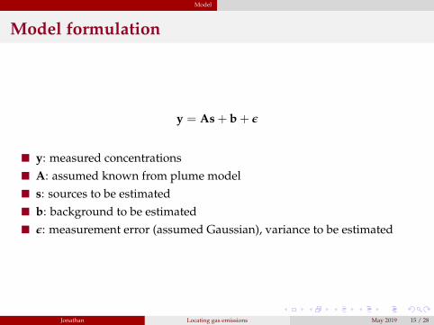
Model formulation

y = As + b +ε

� y: measured concentrations� A: assumed known from plume model� s: sources to be estimated� b: background to be estimated� ε: measurement error (assumed Gaussian), variance to be estimated


Model Plume

Plume model� Red: Source height H� Blue: Source half–width w� Magenta: Downwind offset δR

� Cyan: Horizontal offset δH

� Green: Vertical offset δV

� ABL height: D� Horizontal extent:

σH = δR tan(γH) + w� Vertical extent: σV = δR tan(γV)

� Opening angles: γH , γV

a =1

2π |U|σHσVexp

{−

δ2H

2σ2H

}×

{exp

{− (δV − H)2

2σ2V

}+ exp

{− (δV+H)2

2σ2V

}+ exp

{− (2D− δV − H)2

2σ2V

}+ exp

{− (2D− δV + H)2

2σ2V

} }


Model Background

Background model

Requirements� Positive and smoothly–varying, spatially and temporally� Basis function representation: b = Pβ� We use Gaussian Markov random field� Explicit spatial dependence due to wind transport incorporated

Random field prior

f (β) ∝ exp{−µ2 (β−β0)

TJβ(β−β0)}

� Jβ is sparse, P = I� Fast estimation


Inference Str

Inference strategy

Initial point estimation� Sources and background� Source locations assumed on fixed grid� Fast estimation of starting solution for Bayesian inference

Subsequent Bayesian inference� Sources, background, measurement error, wind–field parameters, ...� Grid-free sources modelled using Gaussian mixture model� Reversible jump MCMC inference� Quantified parameter uncertainties and dependencies


Inference PntEst

Initial point estimation

Background prior

f (β) ∝ exp{−µ2 (β−β0)

TJβ(β−β0)}

Source prior (Laplace)f (s) ∝ exp{−λ‖Qs‖1}

Likelihoodf (y|s,β) ∝ exp{− 1

2σ2ε‖As + Pβ− y‖2},

Posteriorf (s,β|y) ∝ f (y|s,β) f (s) f (β)

Maximum a-posteriori estimate

argmins,β1

2σ2ε‖As + Pβ− y‖2 + µ

2 (β−β0)T J(β−β0) + λ‖Qs‖1


Inference BsnInf

Bayesian inferenceParameters� Source locations z, “widths” w and emission rates s for mixture of m

sources� Random field background parameters β� Measurement error standard deviation σε

� Wind–direction correction δφ

� Others (e.g. plume opening angles)� Call theseθ which can be partitioned {θκ ,θκ}

Full conditionalf (θκ |y,θκ) ∝ f (y|θκ ,θκ) f (θκ |θκ)

Inference tools� Gibbs’ sampling� Reversible jump� (Metropolis–Hastings)


Results Synthetic

Synthetic

(a) initial (b) median (c) 2.5% (d) 97.5%


Results Landfill

Landfill

(a) initial (b) median (c) 2.5% (d) 97.5%


Results Flare stack

Flare stack

(a) initial (b) median (c) 2.5% (d) 97.5%Jonathan Locating gas emissions May 2019 23 / 28

Results Flare stack

Flare stack

(a) background in time (b) residual vs measured concentrationinitial (red); posterior median (black)

Wind direction correction of 18o


Conclusions

Conclusions and on–going work

Conclusions� Data structure and management� Flexible inference using combination of standard methods� Good performance on synthetic and field applications� Scalability from iterative estimation

Extensions (on-going and potential)� Multiple flights, multiple wind data sources� Enhanced plume model� Internal calibration� Improved prior characterisation of sources, intermittent sources� Simultaneous inference using multiple measurement types� Optimal design� Line-of-sight and satellite applications

Slides and articles at www.lancs.ac.uk/∼jonathan


Conclusions

Line-of-sight sensing

Line-of-sight laser


Conclusions

Satellite

Tropomi satellite and Google Earth


Conclusions

Satellite Service Dates

Potential to measure individual sources


Date post:	03-Feb-2022
Category:	Documents
Upload:	others
View:	4 times
Download:	0 times

Locating and quantifying gas emission sources using ...

Documents