MNRAS 000, 1–14 (2016) Preprint 23 June 2016 Compiled using MNRAS LATEX style file v3.0

LOFAR VLBI Studies at 55MHz of 4C 43.15, a z=2.4 RadioGalaxy

Leah K. Morabito1?, Adam T. Deller2, Huub Röttgering1, George Miley1, Es-kil Varenius3, Timothy W. Shimwell1, Javier Moldón4, Neal Jackson3, RaffaellaMorganti2,5, Reinout J. van Weeren6, J. B. R. Oonk1,2

1Leiden Observatory, P.O. Box 9513, 2300 RA, Leiden, The Netherlands2Netherlands Institute for Radio Astronomy (ASTRON), Postbus 2, 7990 AA Dwingeloo, The Netherlands3Department of Earth and Space Sciences, Chalmers University of Technology, Onsala Space Observatory, 439 92 Onsala, Sweden4Jodrell Bank Centre for Astrophysics, School of Physics and Astronomy, University of Manchester, Oxford Road, Manchester M13 9PL, UK5Kapteyn Astronomical Institute, University of Groningen, P.O. Box 800, 9700 AV Groningen, The Netherlands6Harvard-Smithsonian Center for Astrophysics, 60 Garden Street, Cambridge, MA 02138, USA

ABSTRACTThe correlation between radio spectral index and redshift has been exploited to dis-cover high redshift radio galaxies, but its underlying cause is unclear. It is crucialto characterise the particle acceleration and loss mechanisms in high redshift radiogalaxies to understand why their radio spectral indices are steeper than their localcounterparts. Low frequency information on scales of ∼ 1 arcsec are necessary todetermine the internal spectral index variation. In this paper we present the first spa-tially resolved studies at frequencies below 100MHz of the z = 2.4 radio galaxy 4C43.15 which was selected based on its ultra-steep spectral index (α < −1; Sν ∼ να)between 365MHz and 1.4GHz. Using the International Low Frequency Array (LO-FAR) Low Band Antenna we achieve sub-arcsecond imaging resolution at 55MHz withVLBI techniques. Our study reveals low-frequency radio emission extended along thejet axis, which connects the two lobes. The integrated spectral index for frequencies< 500MHz is -0.83. The lobes have integrated spectral indices of -1.31±0.03 and -1.75±0.01 for frequencies ≥ 1.4GHz, implying a break frequency between 500MHzand 1.4GHz. These spectral properties are similar to those of local radio galaxies.We conclude that the initially measured ultra-steep spectral index is due to a com-bination of the steepening spectrum at high frequencies with a break at intermediatefrequencies.

Key words: galaxies: active – galaxies: jets – radio continuum: galaxies – galaxies:individual: 4C 43.15

1 INTRODUCTION

High redshift radio galaxies (HzRGs) are rare, spectac-ular objects with extended radio jets whose length ex-ceeds scales of a few kiloparsecs. The radio jets are edge-brightened, Fanaroff-Riley class II (FR II; Fanaroff & Riley1974) sources. Found in overdensities of galaxies indicativeof protocluster environments (e.g., Pentericci et al. 2000b),HzRGs are among the most massive galaxies in the distantuniverse and are likely to evolve into modern-day dominantcluster galaxies (Miley & De Breuck 2008; Best et al. 1997).

? E-mail: morabito@strw.leidenuniv.nl

They are therefore important probes for studying the forma-tion and evolution of massive galaxies and clusters at z ≥ 2.

One of the most intriguing characteristics of the rel-ativistic plasma in HzRGs is the correlation between thesteepness of the radio spectra and the redshift of the asso-ciated host galaxy (Tielens et al. 1979; Blumenthal & Miley1979). Radio sources with steeper spectral indices are gener-ally associated with galaxies at higher redshift, and samplesof radio sources with ultra-steep spectra (α . −1 where theflux density S is S ∝ να) were effectively exploited to dis-cover HzRGs (e.g., Röttgering et al. 1994; Chambers et al.1990, 1987).

The underlying physical cause of this relation is still

c© 2016 The Authors

arX

iv:1

606.

0674

1v1

[as

tro-

ph.G

A]

21

Jun

2016

2 Leah K. Morabito

not understood. Three causes have been proposed: observa-tional biases, environmental influences, and internal particleacceleration mechanisms that produce intrinsically steeperspectra.

Several observational biases can impact the measuredrelation. Klamer et al. (2006) explored the radio “k-correction” using a sample of 28 spectroscopically confirmedHzRGs. The authors compared the relation between spec-tral index and redshift as measured from the observed andrest frame spectra, and found that the relation remainedunchanged. Another bias could come from the fact that jetpower and spectral index are correlated. This manifests in anobserved luminosity−redshift correlation: brighter sources(which tend to be at higher redshifts) are more likely to havehigher jet power, and therefore steeper spectral indices. Forflux density limited surveys this leads to a correlation be-tween power and redshift, and surveys with higher flux den-sity limits have a tighter power−redshift correlation (Blun-dell et al. 1999).

Environmental effects could also impact the relation.The temperature of the circumgalactic medium is expectedto be higher at higher redshifts. It is also known that thelinear sizes of radio sources decrease with redshift (e.g., Mi-ley 1968; Neeser et al. 1995) which is interpreted as lowerexpansion speeds due to higher surrounding gas densities athigher redshifts. Athreya & Kapahi (1998) point out that theexpanding radio lobes therefore have to work against higherdensity and temperature. This would slow down the prop-agation of the jet into the medium, increasing the Fermiacceleration and thus steepening the spectral index. Thepower−redshift correlation in this case would be caused bya change in environment with redshift.

The final option is that the steeper spectrum is indica-tive of particle acceleration mechanisms different from thosein local radio galaxies. One global difference between lowand high redshift sources is that the CMB temperature ishigher, and could provide more inverse Compton losses athigh frequencies from scattering with CMB photons. Inter-nally to a radio galaxy, spectral indices are seen to evolvealong the radio jet axis, with hot spots dominant at highfrequencies, and diffuse lobe emission is dominant at lowfrequencies (e.g. Cygnus A; Carilli et al. 1991). RecentlyMcKean et al. (2016) observed a turnover in the spectra ofthe hot spots detected with LOFAR around 100MHz. Theauthors were able to rule out a cut off in the low-energy elec-tron distribution, and found that both free-free absorptionor synchrotron self-absorption models provided adequate fitsto the data, albeit with unlikely model parameters. To de-termine the particle acceleration mechanisms it is crucialto make observations at 100MHz and below with sufficientresolution to determine the internal variation of the low-frequency spectra. This can then be compared to archivalobservations with similar or higher resolution at frequenciesabove 1GHz, where the internal structure of HzRGs havebeen well studied (e.g., Carilli et al. 1997; Pentericci et al.2000a). All current low frequency information that does ex-ist comes from studies in which HzRGs are unresolved.

Typical angular sizes of HzRGs with z & 2 are about10 arcsec (Wardle & Miley 1974), driving the need for reso-lutions of about an arcsecond to determine the distributionof spectral indices among spatially resolved components ofHzRGs. The unique capabilities of the Low Frequency Ar-

ray (LOFAR; van Haarlem et al. 2013) are ideally suitedfor revealing these distributions at low frequencies. Cover-ing the frequency bands of 10–80MHz (Low Band Antenna;LBA) and 120–240MHz (High Band Antenna; HBA), LO-FAR can characterize HzRG spectra down to rest frequen-cies of ∼ 100MHz. The full complement of stations compris-ing International LOFAR (I-LOFAR) provides baselines over1000 km, and sub-arcsecond resolution is achievable down tofrequencies of about 60MHz.

At such low radio frequencies, very long baseline inter-ferometry (VLBI) becomes increasingly challenging, as sig-nal propagation through the ionosphere along the differentsightlines of widely separated stations gives rise to large dif-ferential dispersive delays. These vary rapidly both in timeand with direction on the sky, requiring frequent calibrationsolutions interpolated to the position of the target. Previousworks have focused on observations at ∼ 150MHz where I-LOFAR is most sensitive and the dispersive delays are lessproblematic (Varenius et al. 2015, Varenius et al., A&A sub-mitted). The ν−2 frequency dependence of the ionosphericdelays means they are six times larger at 60MHz than at150MHz, reducing the bandwidth over which the assump-tion can be made that the frequency dependence is linear.Combined with the lower sensitivity of I-LOFAR in the LBAband and the reduction in the number of suitable calibrationsources due to absorption processes in compact radio sourcesbelow 100MHz, this makes reducing LBA I-LOFAR obser-vations considerably more challenging than HBA observa-tions. Accordingly, the LBA band of I-LOFAR has been lessutilised than the HBA. Previous published LBA results havebeen limited to observations of 3C 196 (Wucknitz 2010) andthe Crab nebula (unpublished) during LOFAR commission-ing, when the complement of operational stations limitedthe longest baseline to ∼600 km.

Here we use I-LOFAR to study the spatially resolvedproperties of 4C 43.15 (also B3 0731+438) at z = 2.429(McCarthy 1991). This object is one of a sample of 10 thatcomprise a pilot study of the ultra-steep spectra of HzRGs.We selected 4C 43.15 for this study based on data qual-ity, the suitability of the calibrator, and the simple double-lobed, edge-brightened structure of the target seen at higherfrequencies. The overall spectral index of 4C 43.15 between365 MHz (Texas Survey of Radio Sources; Douglas et al.1996) and 1400 MHz (from the Green Bank 1.4 GHz North-ern Sky Survey; White & Becker 1992) is α = −1.1, whichplaces it well within the scatter on the α − z relation, seenin Figure 1 of De Breuck et al. (2000). 4C 43.15 has beenwell studied at optical frequencies, and exhibits many of thecharacteristics of HzRGs (e.g., an extended Lyman-α halo;Villar-Martín et al. 2003).

Here we present images of 4C 43.15 made with the LBAof I-LOFAR at 55MHz. These are the first images made withthe full operational LBA station complement of I-LOFARin 2015, and this study sets the record for image resolutionat frequencies less than 100MHz. We compare the low fre-quency properties of 4C 43.15 with high frequency archivaldata from the Very Large Array (VLA) to measure the spec-tral behaviour from 55 – 4860MHz. We describe the calibra-tion strategy we designed to address the unique challenges ofVLBI for the LBA band of I-LOFAR. The calibration strat-egy described here provides the foundation for an ongoing

MNRAS 000, 1–14 (2016)

4C 43.15 at 55MHz 3

pilot survey of ten HzRGs in the Northern Hemisphere withultra steep (α < −1) spectra.

In § 2 we outline the observations and data pre-processing. Section 3 describes the LBA calibration, includ-ing the VLBI techniques. The resulting images are pre-sented in § 4 and discussed in § 5. The conclusions andoutlook are summarised in § 6. Throughout the paper weassume a ΛCDM concordance cosmology with H0 = 67.8km s−1 Mpc−1, Ωm = 0.308, and ΩΛ = 0.692, consistentwith Planck Collaboration et al. (2015). At the distance of4C 43.15, 1′′corresponds to 8.32 kpc.

2 OBSERVATIONS AND PRE-PROCESSING

In this section we describe the observations, pre-processingsteps and initial flagging of the data.

As part of project LC3_018, the target 4C 43.15 was ob-served on 22 Jan 2015 with 8.5 hr on-source time. Using twobeams we conducted the observation with simultaneous con-tinuous frequency coverage between 30 and 78MHz on boththe target and a flux density calibrator. Designed with cal-ibration redundancy in mind, the observation started with3C 147 as the calibrator and switched to 3C 286 halfwaythough the observation. Although 3C286 was included forcalibrator redundancy, it was later realised that the largeuncertainties of the current available beam models preventaccurate calibration transfer to the target at this large angu-lar separation. The observations are summarized in Table 1.

All 46 operational LBA stations participated in the ob-servation, including 24 core stations, 14 remote stations,and 8 international stations. The international stations in-cluded 5 in Germany (DE601-DE605) and one each in Swe-den (SE607), France (FR606), and the United Kingdom(UK608). While all stations have 96 dipoles, the core andremote stations are limited by electronics to only using48 dipoles at one time. The observation was made in theLBA_OUTER configuration, which uses only the outermost48 dipoles in the core and remote stations. This configura-tion reduces the amount of cross-talk between closely spaceddipoles and gives a smaller field of view when compared withother configurations. The international stations always useall 96 dipoles, and thus have roughly twice the sensitivity ofcore and remote stations. The raw data were recorded withan integration time of 1 s and 64 channels per 0.195MHzsubband to facilitate radio frequency interference (RFI) ex-cision.

2.1 Radio Observatory Processing

All data were recorded in 8-bit mode and correlated with theCOBALT correlator to produce all linear correlation prod-ucts (XX, XY, YX, YY). After correlation the data werepre-processed by the Radio Observatory. Radio frequencyinterference was excised using AOFlagger (Offringa 2010)with the default LBA flagging strategy. The data were aver-aged to 32 channels per subband (to preserve spectral reso-lution for future studies of carbon radio recombination lines)and 2 second integration time (to preserve information onthe time-dependence of phases) before being placed in theLong Term Archive (LTA). The data were retrieved from theLTA and further processed on a parallel cluster kept up to

date with the most current stable LOFAR software availableat the time (versions 2.9 – 2.15).

3 DATA CALIBRATION

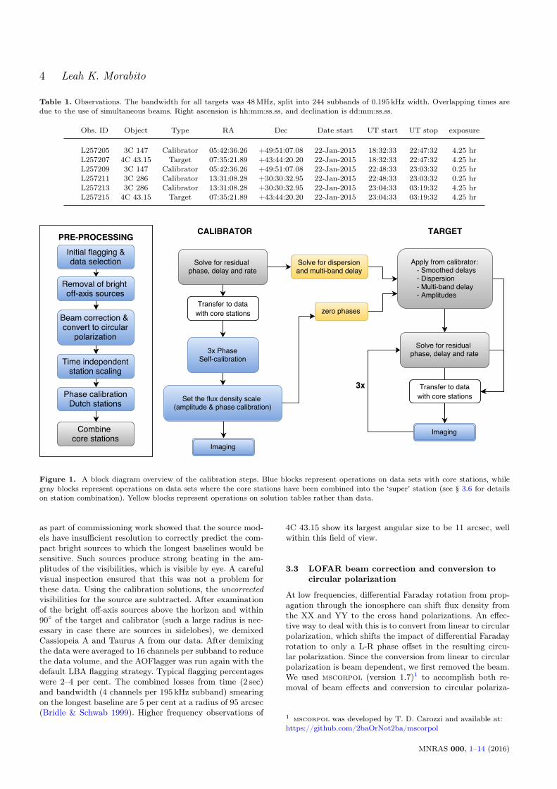
In this section we describe in detail the steps taken to cali-brate the entire LBA, including international stations, pay-ing particular attention to how we address the unique chal-lenges at low frequencies. Figure 1 shows a block diagramoverview of the calibration steps.

3.1 Initial flagging and data selection

Our first step after downloading the data from the LTA wasto run AOFlagger again with the LBA default strategy. Typ-ically 0.5 to 2 per cent of the data in each subband wereflagged. An inspection of gain solutions from an initial gaincalibration of the entire bandwidth on 3C 147 showed thatthe Dutch remote station RS409 had dropped out halfwaythrough the first observing block, and we flagged this sta-tion and removed it from the dataset. We further excisedone core station (CS501) and one remote station (RS210)after manual inspection.

We determined the normalised standard deviation persubband from the calibrator data and used this informationto select the most sensitive subbands close to the peak sen-sitivity of the LBA. Outside these subbands the normalisedstandard deviation rapidly increases towards the edges ofthe frequency range. The total contiguous bandwidth se-lected was 15.6MHz with a central frequency of 55MHz.During this half of the observation, the standard calibrator3C 147 was always less than 20 degrees in total angular sep-aration from the target, and the absolute flux density errorsare expected to be less than 20 per cent. This is importantfor two reasons. First, amplitude errors from beam correc-tion models are reduced when objects are close in elevation.The second reason is that we transfer information derivedfrom the calibrator phases (see § 3.10 for full details) to thetarget. This information is valid for a particular directionon the sky, and transferral over very large distances will notimprove the signal to noise ratio for the target data. For thesecond half of the observation, 3C 286 was more than 20degrees distant from 4C 43.15 for most of that observationblock, requiring more advanced calibration which is beyondthe scope of this paper, and would only provide

√2 noise im-

provement. The second half of the observation was thereforenot used for the data analysis in this paper.

3.2 Removal of bright off-axis sources

Bright off-axis sources contribute significantly to the visi-bilities. At low frequencies, this problem is exacerbated byLOFAR’s wide field of view and large primary beam side-lobes. There are several sources that have brightnesses ofthousands to tens of thousands of Janskys within the LBAfrequency range, and they need to be dealt with. We accom-plished the removal of bright off-axis sources using a methodcalled demixing (van der Tol et al. 2007), where the dataare phase-shifted to the off-axis source, averaged to mimicbeam and time smearing, and calibrated against a model.All baselines were demixed, although simulations performed

MNRAS 000, 1–14 (2016)

4 Leah K. Morabito

Table 1. Observations. The bandwidth for all targets was 48MHz, split into 244 subbands of 0.195 kHz width. Overlapping times aredue to the use of simultaneous beams. Right ascension is hh:mm:ss.ss, and declination is dd:mm:ss.ss.

Obs. ID Object Type RA Dec Date start UT start UT stop exposure

L257205 3C 147 Calibrator 05:42:36.26 +49:51:07.08 22-Jan-2015 18:32:33 22:47:32 4.25 hrL257207 4C 43.15 Target 07:35:21.89 +43:44:20.20 22-Jan-2015 18:32:33 22:47:32 4.25 hrL257209 3C 147 Calibrator 05:42:36.26 +49:51:07.08 22-Jan-2015 22:48:33 23:03:32 0.25 hrL257211 3C 286 Calibrator 13:31:08.28 +30:30:32.95 22-Jan-2015 22:48:33 23:03:32 0.25 hrL257213 3C 286 Calibrator 13:31:08.28 +30:30:32.95 22-Jan-2015 23:04:33 03:19:32 4.25 hrL257215 4C 43.15 Target 07:35:21.89 +43:44:20.20 22-Jan-2015 23:04:33 03:19:32 4.25 hr

Figure 1. A block diagram overview of the calibration steps. Blue blocks represent operations on data sets with core stations, whilegray blocks represent operations on data sets where the core stations have been combined into the ‘super’ station (see § 3.6 for detailson station combination). Yellow blocks represent operations on solution tables rather than data.

as part of commissioning work showed that the source mod-els have insufficient resolution to correctly predict the com-pact bright sources to which the longest baselines would besensitive. Such sources produce strong beating in the am-plitudes of the visibilities, which is visible by eye. A carefulvisual inspection ensured that this was not a problem forthese data. Using the calibration solutions, the uncorrectedvisibilities for the source are subtracted. After examinationof the bright off-axis sources above the horizon and within90 of the target and calibrator (such a large radius is nec-essary in case there are sources in sidelobes), we demixedCassiopeia A and Taurus A from our data. After demixingthe data were averaged to 16 channels per subband to reducethe data volume, and the AOFlagger was run again with thedefault LBA flagging strategy. Typical flagging percentageswere 2–4 per cent. The combined losses from time (2 sec)and bandwidth (4 channels per 195 kHz subband) smearingon the longest baseline are 5 per cent at a radius of 95 arcsec(Bridle & Schwab 1999). Higher frequency observations of

4C 43.15 show its largest angular size to be 11 arcsec, wellwithin this field of view.

3.3 LOFAR beam correction and conversion tocircular polarization

At low frequencies, differential Faraday rotation from prop-agation through the ionosphere can shift flux density fromthe XX and YY to the cross hand polarizations. An effec-tive way to deal with this is to convert from linear to circularpolarization, which shifts the impact of differential Faradayrotation to only a L-R phase offset in the resulting circu-lar polarization. Since the conversion from linear to circularpolarization is beam dependent, we first removed the beam.We used mscorpol (version 1.7)1 to accomplish both re-moval of beam effects and conversion to circular polariza-

1 mscorpol was developed by T. D. Carozzi and available at:https://github.com/2baOrNot2ba/mscorpol

MNRAS 000, 1–14 (2016)

4C 43.15 at 55MHz 5

tion. This software performs a correction for the geometricprojection of the incident electric field onto the antennas,which are modelled as ideal electric dipoles. One drawbackof mscorpol is that it does not yet include frequency de-pendence in the beam model, so we also replicated our en-tire calibration strategy but correcting for the beam withthe LOFAR new default pre-processing pipeline (NDPPP),which has frequency-dependent beam models, rather thanmscorpol. We converted the NDPPP beam-corrected datato circular polarization using standard equations, and fol-lowed the same calibration steps described below. We foundthat data where the beam was removed with mscorpol ul-timately had more robust calibration solutions and betterreproduced the input model for the calibrator. Therefore wechose to use the mscorpol beam correction.

3.4 Time-independent station scaling

The visibilities for the international stations must be scaledto approximately the right amplitudes relative to the coreand remote stations before calibration. This is importantbecause the amplitudes of the visibilities are later used tocalculate the data weights, which are used in subsequent cal-ibration steps, see § 3.7. To do this we solved for the diagonalgains (RR,LL) on all baselines using the Statistical EfficientCalibration (StEfCal; Salvini & Wijnholds 2014) algorithmin NDPPP. One solution was calculated every eight secondsper 0.915MHz bandwidth (one subband). The StEfCal al-gorithm calculates time and frequency independent phaseerrors, and does not take into account how phase changeswith frequency (the delay; dφ/dν) or time (the rate; dφ/dt).If the solution interval over which StEfCal operates is largecompared to these effects, the resulting incoherent averagingwill result in a reduction in signal to noise. Since the incoher-ently averaged amplitudes are adjusted to the correct level,the coherence losses manifest as an increase of the noiselevel. Using the maximal values for delays and rates foundin § 3.7 to calculate the signal to noise reduction (from Eqn.9.8 and 9.11 of Moran & Dhawan 1995), we find losses of 6and 16 per cent for delays and rates, respectively.

The calibrator 3C 147 flux density was given by themodel from Scaife & Heald (2012). 3C 147 is expected tobe unresolved or only marginally resolved and therefore ex-peted to provide an equal amplitude response to baselinesof any length. We use this gain calibration for two tasks: (i)to find an overall scaling factor for each station that cor-rectly provides the relative amplitudes of all stations; and(ii) to identify bad data using the LOFAR Solution Tool2.About 20 per cent of the solutions were flagged either dueto outliers or periods of time with loss of phase coherence,and we transferred these flags back to the data. To find thetime-independent scaling factor per station, we zeroed thephases and calculated a single time-averaged amplitude cor-rection for each antenna. These corrections were applied toboth calibrator and target datasets.

2 The LOFAR Solution Tool (LoSoTo) was developed byFrancesco de Gasperin and is available at:https://github.com/revoltek/losoto

3.5 Phase calibration for Dutch stations

We solved for overall phase corrections using only the Dutcharray but filtering core – core station baselines, which canhave substantial low-level RFI and are sensitive to extendedemission. The phase calibration removes ionospheric distor-tions in the direction of the dominant source at the pointingcentre. We performed the phase calibration separately for3C 147 and 4C 43.15 using appropriate skymodels. 3C 147is the dominant source in its field, and we use the Scaife &Heald (2012) point source model. 4C 43.15 has a flux densityof at least 10 Jy in the LBA frequency range. We used anapparent sky model of the field constructed from the TGSSAlternative Data Release 1 (Intema et al. 2016), containingall sources within 7 degrees of our target and with a fluxdensity above 1 Jy.

3.6 Combining core stations

After phase calibration of the Dutch stations for both thecalibrator and the target, we coherently added the visi-bilities from the core stations to create a ‘super’ station.This provides an extremely sensitive ‘super’ station with in-creased signal to noise on individual baselines to anchor theI-LOFAR calibration (described further in § 3.7). All corestations are referred to a single clock and hence should havedelays and rates that are negligibly different after phase cal-ibration is performed. The station combination was accom-plished with the Station Adder in NDPPP by taking theweighted average of all visibilities on particular baselines.For each remote and international station, all visibilities onbaselines between that station and the core stations are av-eraged together taking the data weights into account. Thenew u, v, w coordinates are calculated as the weighted ge-ometric center of the u, v, w coordinates of the visibilitiesbeing combined3. Once the core stations were combined, wecreated a new data set containing only the ‘super’ stationand remote and international stations. The dataset with theuncombined core stations was kept for later use. The final av-eraging parameters for the data were 4 channels per subbandfor 3C 147, and 8 channels per subband for 4C 43.15. Afteraveraging the data were again flagged with the AOFlaggerdefault LBA flagging strategy, which flagged another 1 – 2per cent of the data.

3.7 Calibrator residual phase, delay, and rate

The international stations are separated by up to 1292 kmand have independent clocks which time stamp the dataat the correlator. There are residual non-dispersive delaysdue to the offset of the separate rubidium clocks at eachstation. Correlator model errors can also introduce residualnon-dispersive delays up to ∼ 100ns. Dispersive delays fromthe ionosphere make a large contribution to the phase er-rors. Given enough signal to noise on every baseline, wecould solve for the phase errors over small enough time

3 We found an extra 1 per cent reduction in noise for the cal-ibrator when using the weighted geometric center of the u, v, wcoordinates, rather than calculating the u, v, w coordinates basedon the ‘super’ station position. This has been implemented inNDPPP (LOFAR software version 12.2.0)

MNRAS 000, 1–14 (2016)

6 Leah K. Morabito

and bandwidth intervals that the dispersive errors can beapproximated as constant. However, a single international-international baseline is only sensitive to sources of ∼ 10Jyover the resolution of our data (∆ν = 0.195MHz, 2 sec).Larger bandwidth and time intervals increase the signal tonoise ratio, and the next step is to model the dispersive de-lays and rates with linear slopes in frequency and time. Thiscan be done using a technique known as fringe-fitting (e.g.,Cotton 1995; Thompson et al. 2001). A global fringe-fittingalgorithm is implemented as the task FRING in the As-tronomical Image Processing System (AIPS; Greisen 2003).We therefore converted our data from measurement set toUVFITS format using the task ms2uvfits and read it intoAIPS. The data weights of each visibility were set to be theinverse square of the standard deviation of the data withina three minute window.

The ionosphere introduces a dispersive delay, wherethe phase corruption from the ionosphere is inversely pro-portional to frequency, φion ∝ ν−1. The dispersive de-lay is therefore inversely proportional to frequency squared,dφ/dν ∝ −ν−2. Non-dispersive delays such as those intro-duced by clock offsets are frequency-independent. The iono-spheric delay is by far the dominant effect. For a more in-depth discussion of all the different contributions to the de-lay at 150MHz for LOFAR, see Moldón et al. (2015). The de-lay fitting-task FRING in AIPS fits a single, non-dispersivedelay solution to each so-called intermediate frequency (IF),where an IF is a continuous bandwidth segment. With I-LOFAR data, we have the freedom to choose the desired IFbandwidth by combining any number of LOFAR subbands(each of width 0.195MHz). This allows us to make a piece-wise linear approximation to the true phase behaviour. Mak-ing wider IFs provides a higher peak sensitivity, but leadsto increasingly large deviations between the (non-dispersiveonly) model and the (dispersive and non-dispersive) realityat the IF edges when the dispersive delay contribution islarge. As a compromise, we create 8 IFs of width 1.95MHzeach (10 LOFAR subbands), and each IF is calibrated inde-pendently. We used high resolution model of 3C 147 (froma previous I-LOFAR HBA observation at 150MHz) for thecalibration, and set the total flux density scale from Scaife& Heald (2012). The solution interval was set to 30 seconds,and we found solutions for all antennas using only baselineswith a projected separation > 10kλ, effectively removingdata from all baselines containing only Dutch stations. Thecalibration used the ‘super’ station as the reference antenna.

The search windows were limited to 5µs for delays and80mHz for rates. Typical delays for remote stations were30 ns, while international station delays ranged from 100 nsto 1µs. The delay solutions showed the expected behaviour,with larger offsets from zero for longer baselines, and increas-ing magnitudes (away from zero) with decreasing frequency.Rates were typically up to a few tens of mHz for remote andinternational stations.

3.8 Calibrator phase self-calibration

The combined ‘super’ station, while useful for gaining sig-nal to noise on individual baselines during fringe-fitting,left undesirable artefacts when imaging. This can occur ifthe phase-only calibration prior to station combination isimperfect. The imperfect calibration will result in the ‘su-

Time from start of observation

Am

plitu

de [c

orre

ctio

n fa

ctor

]00:00:00 01:00:00 02:00:00 03:00:00 04:00:00

0.0

0.5

1.0

1.5

2.0

DE601DE602DE603DE604DE605FR606SE607UK608

Core Stations

Remote Stations

Figure 2. Amplitude solutions for all stations, from the final stepof self-calibration. These are corrections to the initial amplitudecalibration of each station, for the central IF at 53MHz. Thecolours go from core stations (darkest) to international stations(lightest).

per’ station not having a sensitivity equal to the sum ofthe constituent core stations. The ‘super’ station also hasa much smaller field of view than the other stations in thearray. Therefore we transferred the fringe-fitting solutionsto a dataset where the core stations were not combined.

Before applying the calibration solutions we smoothedthe delays and rates with solution intervals of 6 and 12minutes, respectively, after clipping outliers (solutions morethan 20 mHz and 50 ns different from the smoothed valuewithin a 30 minute window for rates and delays, respec-tively). The smoothing intervals were determined by com-paring with the unsmoothed solutions to find the smallesttime window that did not oversmooth the data. We appliedthe solutions to a dataset where the core stations were notcombined. The data were then averaged by a factor of two intime prior to self-calibration to 4 second integration times.We performed three phase-only self-calibration loops withtime intervals of 30 seconds, 8 seconds, and 4 seconds. Fur-ther self-calibration did not improve the image fidelity orreduce the image noise.

3.9 Setting the flux density scale

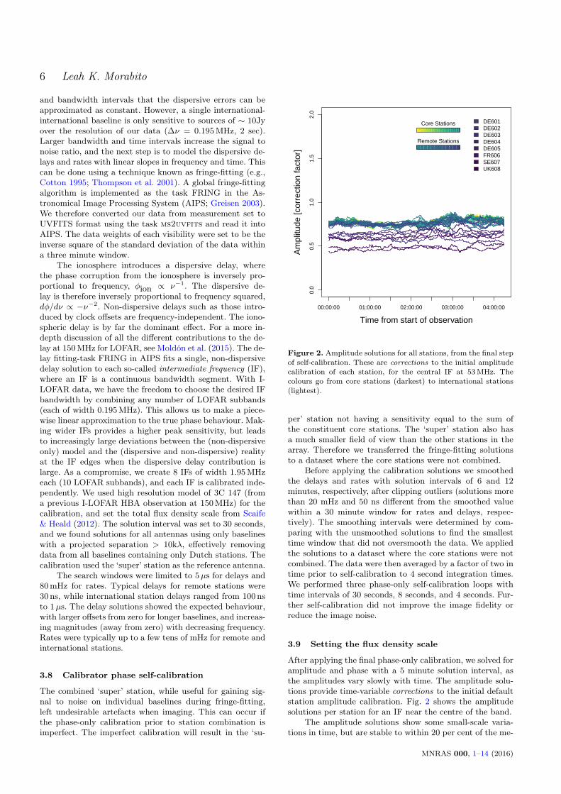
After applying the final phase-only calibration, we solved foramplitude and phase with a 5 minute solution interval, asthe amplitudes vary slowly with time. The amplitude solu-tions provide time-variable corrections to the initial defaultstation amplitude calibration. Fig. 2 shows the amplitudesolutions per station for an IF near the centre of the band.

The amplitude solutions show some small-scale varia-tions in time, but are stable to within 20 per cent of the me-

MNRAS 000, 1–14 (2016)

4C 43.15 at 55MHz 7

dian value over the entirety of the observation. We thereforeadopt errors of 20 per cent for the measurements presentedhere. Several effects could be responsible for the variationsin time such as imperfect beam or source models, or iono-spheric disturbances. Currently we are not able at this timeto distinguish whether the time variation we see is from theionosphere or beam errors.

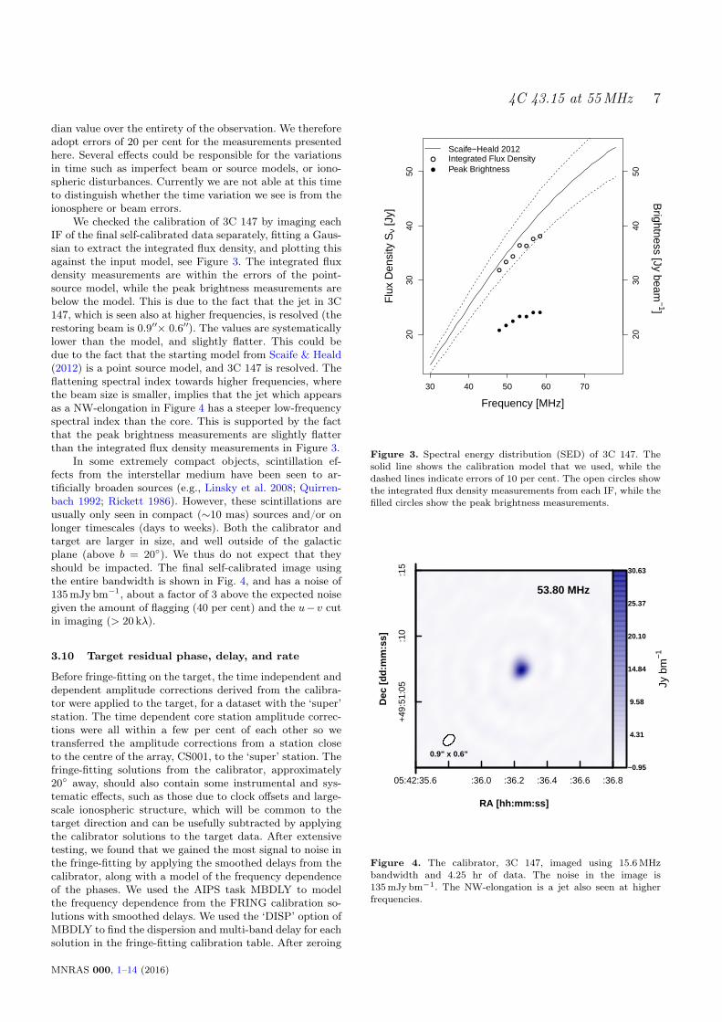
We checked the calibration of 3C 147 by imaging eachIF of the final self-calibrated data separately, fitting a Gaus-sian to extract the integrated flux density, and plotting thisagainst the input model, see Figure 3. The integrated fluxdensity measurements are within the errors of the point-source model, while the peak brightness measurements arebelow the model. This is due to the fact that the jet in 3C147, which is seen also at higher frequencies, is resolved (therestoring beam is 0.9′′× 0.6′′). The values are systematicallylower than the model, and slightly flatter. This could bedue to the fact that the starting model from Scaife & Heald(2012) is a point source model, and 3C 147 is resolved. Theflattening spectral index towards higher frequencies, wherethe beam size is smaller, implies that the jet which appearsas a NW-elongation in Figure 4 has a steeper low-frequencyspectral index than the core. This is supported by the factthat the peak brightness measurements are slightly flatterthan the integrated flux density measurements in Figure 3.

In some extremely compact objects, scintillation ef-fects from the interstellar medium have been seen to ar-tificially broaden sources (e.g., Linsky et al. 2008; Quirren-bach 1992; Rickett 1986). However, these scintillations areusually only seen in compact (∼10 mas) sources and/or onlonger timescales (days to weeks). Both the calibrator andtarget are larger in size, and well outside of the galacticplane (above b = 20). We thus do not expect that theyshould be impacted. The final self-calibrated image usingthe entire bandwidth is shown in Fig. 4, and has a noise of135mJybm−1, about a factor of 3 above the expected noisegiven the amount of flagging (40 per cent) and the u−v cutin imaging (> 20 kλ).

3.10 Target residual phase, delay, and rate

Before fringe-fitting on the target, the time independent anddependent amplitude corrections derived from the calibra-tor were applied to the target, for a dataset with the ‘super’station. The time dependent core station amplitude correc-tions were all within a few per cent of each other so wetransferred the amplitude corrections from a station closeto the centre of the array, CS001, to the ‘super’ station. Thefringe-fitting solutions from the calibrator, approximately20 away, should also contain some instrumental and sys-tematic effects, such as those due to clock offsets and large-scale ionospheric structure, which will be common to thetarget direction and can be usefully subtracted by applyingthe calibrator solutions to the target data. After extensivetesting, we found that we gained the most signal to noise inthe fringe-fitting by applying the smoothed delays from thecalibrator, along with a model of the frequency dependenceof the phases. We used the AIPS task MBDLY to modelthe frequency dependence from the FRING calibration so-lutions with smoothed delays. We used the ‘DISP’ option ofMBDLY to find the dispersion and multi-band delay for eachsolution in the fringe-fitting calibration table. After zeroing

30 40 50 60 70

2030

4050

2030

4050

Frequency [MHz]F

lux

Den

sity

Sν

[Jy]

Brightness [Jy beam

−1]

Scaife−Heald 2012Integrated Flux DensityPeak Brightness

Figure 3. Spectral energy distribution (SED) of 3C 147. Thesolid line shows the calibration model that we used, while thedashed lines indicate errors of 10 per cent. The open circles showthe integrated flux density measurements from each IF, while thefilled circles show the peak brightness measurements.

RA [hh:mm:ss]

Dec

[dd:

mm

:ss]

−0.95

4.31

9.58

14.84

20.10

25.37

30.63

Jy b

m−1

05:42:35.6 :36.0 :36.2 :36.4 :36.6 :36.8

+49

:51:

05:1

0:1

5

0.9" x 0.6"

53.80 MHz

Figure 4. The calibrator, 3C 147, imaged using 15.6MHzbandwidth and 4.25 hr of data. The noise in the image is135mJybm−1. The NW-elongation is a jet also seen at higherfrequencies.

MNRAS 000, 1–14 (2016)

8 Leah K. Morabito

the phases and rates in the FRING calibration solutions, weused the MBDLY results to correct for the multi-band de-lay and the dispersion. With the phases already zeroed, thedispersion provides a relative correction of the phases, effec-tively removing the frequency dependence. This allowed usto use a wider bandwidth in the FRING algorithm, whichincreased the signal to noise. We chose to use the entire15.6MHz bandwidth. The resultant delays were smaller byat least a factor of two on the longest baselines, which wasexpected as transferring the delays from the calibrator al-ready should have corrected the bulk of the delays. Theseresidual delays are then the difference in the dispersion andmulti-band delays between the target and the calibrator.We also tested the effect of only including data from partialuv selections and established that it was necessary to usethe full uv range to find robust fringe-fitting solutions. It isimportant to remember that the shortest baseline is fromthe ‘super’ station to the nearest remote station. There are12 remote station – ‘super’ station baselines, ranging fromabout 4 km to 55 km, with a median length of about 16 km.

The next step was to perform fringe fitting on the tar-get. We began fringe fitting using a point source modelwith a flux density equal to the integrated flux density ofthe target measured from a low-resolution image made withonly the Dutch array. Initial tests showed a double sourcewith similar separation and position angle (PA) as seen for4C 43.15 at higher frequencies, rather than the input pointsource model. We further self-calibrated by using the result-ing image as a starting model for fringe-fitting. We repeatedthis self-calibration until the image stopped improving.

3.11 Astrometric Corrections

The process of fringe frequency fitting does not derive ab-solute phases or preserve absolute positions, only relativeones. To derive the absolute astrometric positions we as-sumed that the components visible in our derived imagescoincided with the components visible on the high-frequencyarchival data for which the absolute astrometry was correct.We centred the low-frequency lobes in the direction perpen-dicular to the jet axis, and along the jet axis we centredthe maximum extent of the low-frequency emission betweenthe maximum extent of the high frequency emission. There-positioning of the source is accurate to within ∼0.6′′as-suming that the total extent of the low-frequency emissionis contained within the total extent of the high-frequencyemission. This positional uncertainty will not affect the fol-lowing analysis.

4 RESULTS

In Figure 5 we present an LBA image of 4C 43.15 whichachieves a resolution of 0.9′′×0.6′′with PA -33 deg and hasa noise level of 59mJy bm−1. This image was made usingmulti-scale CLEAN in the Common Astronomy SoftwareApplications (CASA; McMullin et al. 2007) software pack-age, with Briggs weighting and a robust parameter of -1.5,which is close to uniform weighting and offers higher reso-lution than natural weighting. The contours show the sig-nificance of the detection (starting at 3σ and up to 20σ).This is the first image made with sub-arcsecond resolution

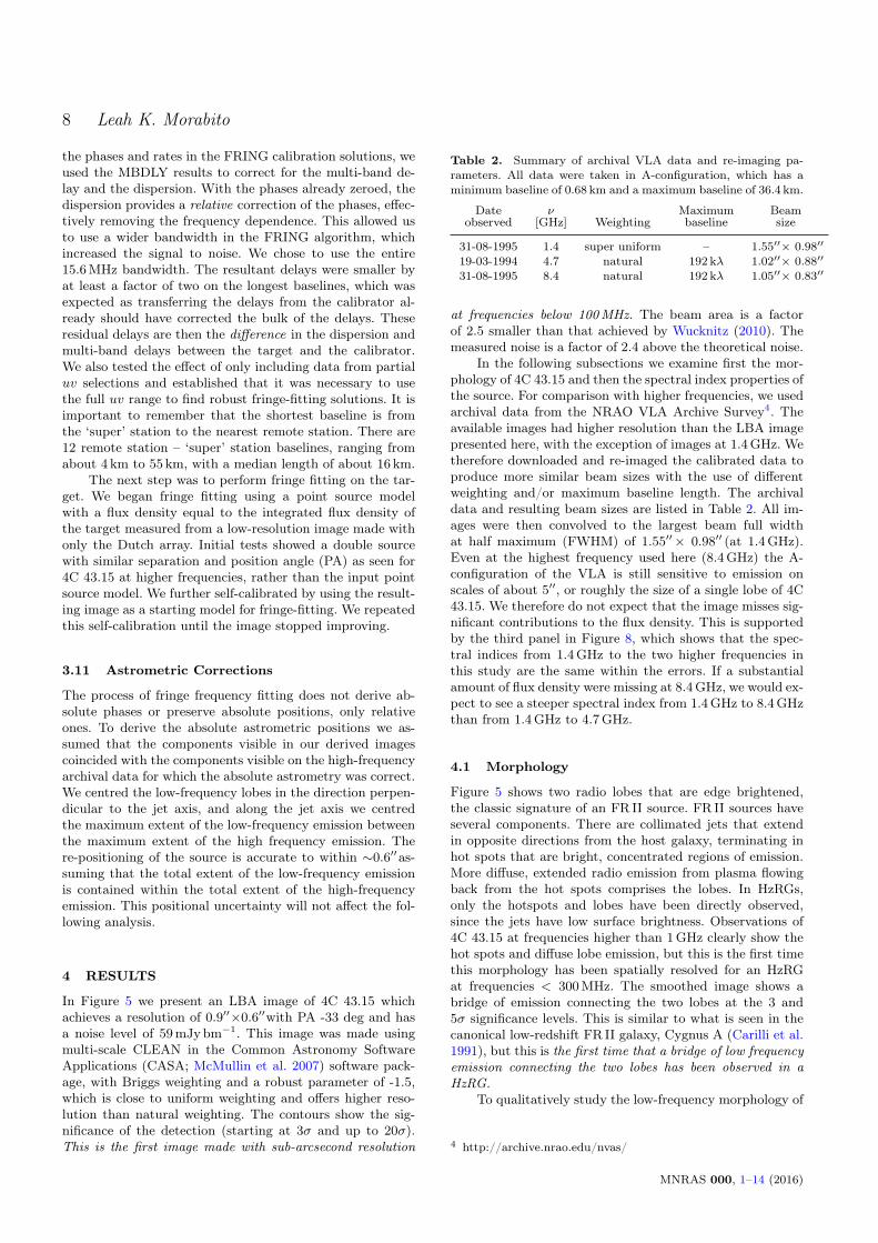
Table 2. Summary of archival VLA data and re-imaging pa-rameters. All data were taken in A-configuration, which has aminimum baseline of 0.68 km and a maximum baseline of 36.4 km.

Date ν Maximum Beamobserved [GHz] Weighting baseline size

31-08-1995 1.4 super uniform – 1.55′′× 0.98′′

19-03-1994 4.7 natural 192 kλ 1.02′′× 0.88′′

31-08-1995 8.4 natural 192 kλ 1.05′′× 0.83′′

at frequencies below 100MHz. The beam area is a factorof 2.5 smaller than that achieved by Wucknitz (2010). Themeasured noise is a factor of 2.4 above the theoretical noise.

In the following subsections we examine first the mor-phology of 4C 43.15 and then the spectral index properties ofthe source. For comparison with higher frequencies, we usedarchival data from the NRAO VLA Archive Survey4. Theavailable images had higher resolution than the LBA imagepresented here, with the exception of images at 1.4GHz. Wetherefore downloaded and re-imaged the calibrated data toproduce more similar beam sizes with the use of differentweighting and/or maximum baseline length. The archivaldata and resulting beam sizes are listed in Table 2. All im-ages were then convolved to the largest beam full widthat half maximum (FWHM) of 1.55′′× 0.98′′ (at 1.4GHz).Even at the highest frequency used here (8.4GHz) the A-configuration of the VLA is still sensitive to emission onscales of about 5′′, or roughly the size of a single lobe of 4C43.15. We therefore do not expect that the image misses sig-nificant contributions to the flux density. This is supportedby the third panel in Figure 8, which shows that the spec-tral indices from 1.4GHz to the two higher frequencies inthis study are the same within the errors. If a substantialamount of flux density were missing at 8.4GHz, we would ex-pect to see a steeper spectral index from 1.4GHz to 8.4GHzthan from 1.4GHz to 4.7GHz.

4.1 Morphology

Figure 5 shows two radio lobes that are edge brightened,the classic signature of an FR II source. FR II sources haveseveral components. There are collimated jets that extendin opposite directions from the host galaxy, terminating inhot spots that are bright, concentrated regions of emission.More diffuse, extended radio emission from plasma flowingback from the hot spots comprises the lobes. In HzRGs,only the hotspots and lobes have been directly observed,since the jets have low surface brightness. Observations of4C 43.15 at frequencies higher than 1GHz clearly show thehot spots and diffuse lobe emission, but this is the first timethis morphology has been spatially resolved for an HzRGat frequencies < 300MHz. The smoothed image shows abridge of emission connecting the two lobes at the 3 and5σ significance levels. This is similar to what is seen in thecanonical low-redshift FR II galaxy, Cygnus A (Carilli et al.1991), but this is the first time that a bridge of low frequencyemission connecting the two lobes has been observed in aHzRG.

To qualitatively study the low-frequency morphology of

4 http://archive.nrao.edu/nvas/

MNRAS 000, 1–14 (2016)

4C 43.15 at 55MHz 9

RA [hh:mm:ss]

Dec

[dd:

mm

:ss]

−0.211

0.088

0.388

0.688

0.988

1.287

1.587

Jy b

m−1

07:35:21 :22 :22 :22 :22 :22

+43

:44:

10:1

5:2

0:2

5:3

0:3

5

0.9" x 0.6"

54.78 MHz

RA [hh:mm:ss]

Dec

[dd:

mm

:ss]

−0.20

0.29

0.78

1.27

1.77

2.26

2.75

Jy b

m−1

07:35:21 :22 :22 :22 :22 :22

+43

:44:

10:1

5:2

0:2

5:3

0:3

51.4" x 1.0"

54.78 MHz

Figure 5. The final LBA images of 4C 43.15. The image on the left was made using 15.6MHz of bandwidth centred on 55MHz. Weused the multi-scale function of the CLEAN task in CASA with Briggs weighting (robust -1.5) and no inner uv cut. The image noiseachieved is 59mJybm−1, while the expected noise given the amount of flagged data and image weighting is 25mJybm−1. The finalrestoring beam is 0.9′′×0.6′′with PA -33 deg. The image on the right is the same image, but smoothed with a Gaussian kernel 1.2 timesthe size of the restoring beam. The contours in both images are drawn at the same levels, which are 3, 5, 10, and 20σ of the unsmoothedimage.

4C 43.15 in more detail and compare it with the structure athigh frequencies, we derived the brightness profiles along andperpendicular to the source axis. To do this we defined thejet axis by drawing a line between the centroids of Gaussianfits to each lobe. We used the position angle of this lineto rotate all images (the unsmoothed image was used forthe 55MHz image) so the jet axis is aligned with North. Wefitted for the rotation angle independently for all frequencies,and found the measured position angles were all within 1degree of each other, so we used the average value of 13.36degrees to rotate all images. The rotated images are shownoverlaid on each other in Figure 6, along with normalizedsums of the flux density along the North–South directionand East–West direction.

The integrated flux density ratio of the lobes alsoevolves with frequency, which can be seen in Figure 6. Thelobe ratio changes from 3 at the highest frequency to 1.7at the lowest frequency. This implies a difference in spectralindex between the two lobes, which will be discussed in thenext section.

4.2 Spectral Index Properties

In this section we shall describe the spectral index proper-ties of 4C 43.15 using the integrated spectra from each ofthe lobes, and the total integrated spectral index. Figure 7shows the lobe spectra and the total integrated spectrum

Table 3. Integrated Flux Density Measurements.

Frequency Flux Density Error Reference[Jy] [Jy]

54MHz 14.9 3.0 This work74MHz 10.6 1.1 VLSS, Cohen et al. (2007)151MHz 5.9 0.17 6C, Hales et al. (1993)178MHz 4.5 0.56 3C, Gower et al. (1967)365MHz 2.9 0.056 Texas, Douglas et al. (1996)408MHz 2.6 0.056 Bologna, Ficarra et al. (1985)750MHz 1.5 0.080 Pauliny-Toth et al. (1966)1.4GHz 0.77 0.023 NVSS, Condon et al. (1998)4.85GHz 0.19 0.029 Becker et al. (1991)

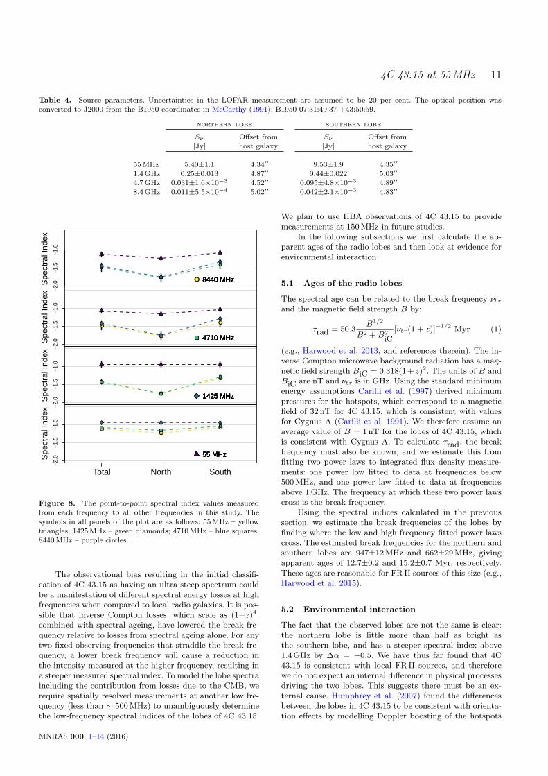
for comparison. The lobe spectra at 1.4, 4.7, and 8.4GHzwere measured from VLA archival images convolved to theresolution at 1.4GHz and are reported in Table 4. We as-sumed errors of 20 per cent for the LOFAR data and 5 percent for the VLA archival data. The integrated spectral datawere taken from the NASA/IPAC Extragalactic Database(NED), with the inclusion of the new LOFAR data point,see Table 3.

Figure 8 shows the point-to-point spectral index valuesmeasured from each frequency to all other frequencies in thisstudy. There are several interesting results.

(i) The spectral index values amongst frequencies ≥1.4GHz show a steepening high-frequency spectrum. This

MNRAS 000, 1–14 (2016)

10 Leah K. Morabito

Index

1

−5 −4 −3 −1 0 1 3 4 5

Relative offset [arcsec]

−8

−6

−4

−2

02

46

8

Rel

ativ

e of

fset

[arc

sec]

1.55" x 0.98"

Index

1N

orm

aliz

edIn

tens

ity

Index

1

NormalizedIntensity

Index1

55 MHz1425 MHz4710 MHz8440 MHz

Figure 6. Contours and intensity profiles for 4C 43.15 at fourfrequencies. The rotation angle of the jet was determined perfrequency to rotate all images so the jet axis is aligned for allimages. The contours are set at 20, 40, 60, 80, and 95 per cent ofthe maximum intensity (which is unity).

can be seen most clearly in the second panel from the top ofFigure 8, where the spectral index from 4.7GHz to 8.4GHzis always steeper than the spectral index from 4.7GHz to1.4GHz for all components.(ii) The point-to-point spectral index from 55MHz to the

higher frequencies in this study steepens, i.e. becomes morenegative, as the other point increases in frequency. This indi-cates a break frequency between 55MHz and 1.4GHz. Thisindicates either a steepening at high frequencies, a turnoverat low frequencies, or a combination of both. However a low-frequency turnover is not observed in the integrated spec-trum. Therefore a steepening of the spectra at high frequen-cies is more likely, which is seen in Figure 7.(iii) The northern lobe always has a spectral index as

steep or steeper than the lobe regardless of the frequenciesused to measure the spectral index. This suggests a physicaldifference between the two lobes.

These results for the entire spectrum are consistent witha flatter, normal FR II spectral index coupled with syn-chrotron losses that steepen the spectra at high frequen-cies and cause a break frequency at intermediate frequencies(Harwood et al., 2016). The spectral index between 55MHzand 1.4GHz is α = −0.95 for both lobes. We fit power lawsto the lobe spectra for frequencies > 1GHz and found spec-tral indices of -1.75±0.01 (northern lobe) and -1.31±0.03(southern lobe). Figure 7 shows six measurements of the to-tal integrated spectrum at frequencies less than 500MHz.The spectral index measured from fitting a power law tothese points is α = −0.83, which we would expect the lobes

50 100 200 500 1000 2000 50000.

010.

050.

505.

00

Frequency [MHz]

Flu

x de

nsity

[Jy

bm−1

]

TotalSouth LobeNorth Lobe

Figure 7. The total integrated spectrum derived from archival(black circles) and LOFAR data (white circle with black outline).The integrated spectra of the lobes are also shown for the mea-surements described in § 4.2. The lines between data points donot represent fits to the data and are only drawn to guide theeye.

to mimic if we had more spatially resolved low-frequencymeasurements.

5 DISCUSSION

The main result is that both the general morphology andspectral index properties of 4C 43.15 are similar to FR IIsources at low redshift. We have determined that 4C 43.15has historically fallen on the spectral index – redshift re-lation because of the steepening of its spectrum at highfrequencies, and a break frequency between 55MHz and1.4GHz. The total integrated spectrum has a spectral indexof α = −0.83±0.02 for frequencies below 500MHz, which isnot abnormally steep when compared to other FR II sources.For example, the median spectral index for the 3CRR sam-ple is α = −0.8 (Laing et al. 1983). The lowest rest frequencyprobed is 180MHz, which is still above where low-frequencyturnovers are seen in the spectra of local FR II sources (e.g.,McKean et al. 2016; Carilli et al. 1991). Thus we expectthe break frequency to be due to synchrotron losses at highfrequencies rather than a low frequency turnover.

We find no evidence that environmental effects cause asteeper overall spectrum. In fact, the northern lobe, whichhas the steeper spectral index, is likely undergoing adia-batic expansion into a region of lower density. This is con-trary to the scenario discussed by Athreya & Kapahi (1998)where higher ambient densities and temperatures will causea steeper spectral index. The interaction of 4C 43.15 with itsenvironment will be discussed in detail later in this section.

MNRAS 000, 1–14 (2016)

4C 43.15 at 55MHz 11

Table 4. Source parameters. Uncertainties in the LOFAR measurement are assumed to be 20 per cent. The optical position wasconverted to J2000 from the B1950 coordinates in McCarthy (1991): B1950 07:31:49.37 +43:50:59.

northern lobe southern lobe

Sν Offset from Sν Offset from[Jy] host galaxy [Jy] host galaxy

55MHz 5.40±1.1 4.34′′ 9.53±1.9 4.35′′

1.4GHz 0.25±0.013 4.87′′ 0.44±0.022 5.03′′

4.7GHz 0.031±1.6×10−3 4.52′′ 0.095±4.8×10−3 4.89′′

8.4GHz 0.011±5.5×10−4 5.02′′ 0.042±2.1×10−3 4.83′′

8440 MHz 8440 MHz 8440 MHz 8440 MHz 8440 MHz 8440 MHz

−2.

0−

1.5

−1.

0

Spe

ctra

l Ind

ex

4710 MHz4710 MHz4710 MHz4710 MHz4710 MHz4710 MHz

−2.

0−

1.5

−1.

0

Spe

ctra

l Ind

ex

1425 MHz1425 MHz1425 MHz1425 MHz1425 MHz1425 MHz

−2.

0−

1.5

−1.

0

Spe

ctra

l Ind

ex

55 MHz55 MHz55 MHz55 MHz55 MHz55 MHz

−2.

0−

1.5

−1.

0

Spe

ctra

l Ind

ex

Total North South

Figure 8. The point-to-point spectral index values measuredfrom each frequency to all other frequencies in this study. Thesymbols in all panels of the plot are as follows: 55MHz – yellowtriangles; 1425MHz – green diamonds; 4710MHz – blue squares;8440MHz – purple circles.

The observational bias resulting in the initial classifi-cation of 4C 43.15 as having an ultra steep spectrum couldbe a manifestation of different spectral energy losses at highfrequencies when compared to local radio galaxies. It is pos-sible that inverse Compton losses, which scale as (1+z)4,combined with spectral ageing, have lowered the break fre-quency relative to losses from spectral ageing alone. For anytwo fixed observing frequencies that straddle the break fre-quency, a lower break frequency will cause a reduction inthe intensity measured at the higher frequency, resulting ina steeper measured spectral index. To model the lobe spectraincluding the contribution from losses due to the CMB, werequire spatially resolved measurements at another low fre-quency (less than ∼ 500MHz) to unambiguously determinethe low-frequency spectral indices of the lobes of 4C 43.15.

We plan to use HBA observations of 4C 43.15 to providemeasurements at 150MHz in future studies.

In the following subsections we first calculate the ap-parent ages of the radio lobes and then look at evidence forenvironmental interaction.

5.1 Ages of the radio lobes

The spectral age can be related to the break frequency νbrand the magnetic field strength B by:

τrad = 50.3B1/2

B2 +B2

iC[νbr(1 + z)]−1/2 Myr (1)

(e.g., Harwood et al. 2013, and references therein). The in-verse Compton microwave background radiation has a mag-netic field strength BiC = 0.318(1+z)2. The units of B andBiC are nT and νbr is in GHz. Using the standard minimumenergy assumptions Carilli et al. (1997) derived minimumpressures for the hotspots, which correspond to a magneticfield of 32 nT for 4C 43.15, which is consistent with valuesfor Cygnus A (Carilli et al. 1991). We therefore assume anaverage value of B = 1nT for the lobes of 4C 43.15, whichis consistent with Cygnus A. To calculate τrad, the breakfrequency must also be known, and we estimate this fromfitting two power laws to integrated flux density measure-ments: one power low fitted to data at frequencies below500MHz, and one power law fitted to data at frequenciesabove 1GHz. The frequency at which these two power lawscross is the break frequency.

Using the spectral indices calculated in the previoussection, we estimate the break frequencies of the lobes byfinding where the low and high frequency fitted power lawscross. The estimated break frequencies for the northern andsouthern lobes are 947±12MHz and 662±29MHz, givingapparent ages of 12.7±0.2 and 15.2±0.7 Myr, respectively.These ages are reasonable for FR II sources of this size (e.g.,Harwood et al. 2015).

5.2 Environmental interaction

The fact that the observed lobes are not the same is clear:the northern lobe is little more than half as bright asthe southern lobe, and has a steeper spectral index above1.4GHz by ∆α = −0.5. We have thus far found that 4C43.15 is consistent with local FR II sources, and thereforewe do not expect an internal difference in physical processesdriving the two lobes. This suggests there must be an ex-ternal cause. Humphrey et al. (2007) found the differencesbetween the lobes in 4C 43.15 to be consistent with orienta-tion effects by modelling Doppler boosting of the hotspots

MNRAS 000, 1–14 (2016)

12 Leah K. Morabito

to predict the resulting asymmetry between the lobes for arange of viewing angles and velocities. Although only hotspot advance speeds of 0.4c and viewing angles of > 20degapproach the measured ∆α = −0.5. Since 4C 43.15 is sim-ilar to Cygnus A, hot spot advance speeds of ∼ 0.05c aremuch more likely. In this scenario, the models in Humphreyet al. (2007) predict a value for ∆α at least an order ofmagnitude smaller than −0.5 for all viewing angles consid-ered. We therefore find it unlikely that orientation is theonly cause for the differences between the lobes.

Environmental factors could also cause differences be-tween the lobes. In lower density environments, adiabaticexpansion of a radio lobe would lower the surface bright-ness, effectively shift the break frequency to lower frequen-cies, and cause a slight steepening of the radio spectrum athigher frequencies. This is consistent with the morphologyand spectral index properties of 4C 43.15. The northern lobeis dimmer, appears more diffuse, and has a spectral indexsteeper than that of the southern lobe. Having ruled outthat orientation can explain these asymmetries, this impliesthat the northern jet is propagating through a lower densitymedium.

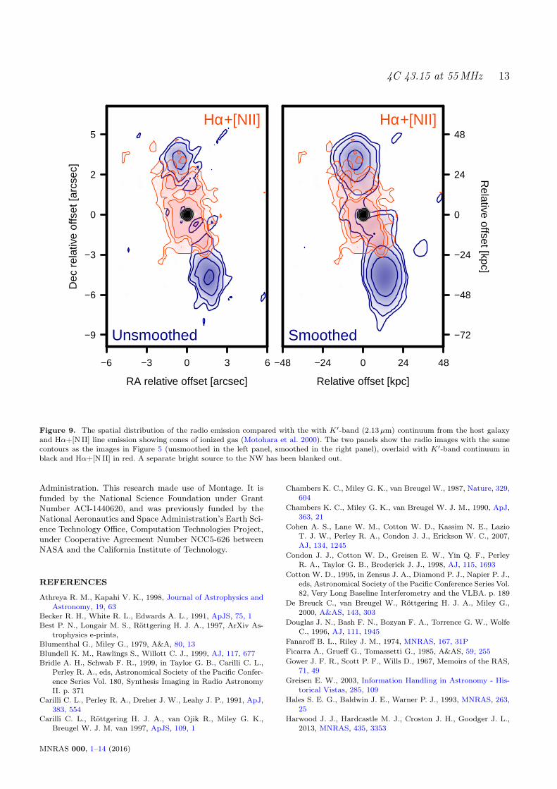
There is supporting evidence for a lower density mediumto the North of the host galaxy. Both Lyman-α (Villar-Martín et al. 2003) and Hα+[NII] (Motohara et al. 2000)are seen to be more extended to the North. Figure 9 showsthe Hα+[NII] overlaid on the radio images for comparison.Qualitatively the emission line gas is more extended and dis-turbed towards the North, and reaches farther into the areaof the radio lobe. Motohara et al. (2000) concluded thatthe Lyman-α and Hα emission are both nebular emissionfrom gas ionized by strong UV radiation from the centralactive galactic nucleus. They estimate the electron densityof the ionised gas to be 38 cm−3 and 68 cm−3 for the north-ern and southern regions, respectively. The lower density inthe North is consistent with adiabatic expansion having alarger impact on the northern lobe relative to the southernlobe. Naively, the ratios between the integrated flux densitiesof the lobes and the densities of the environment are similar.However determining the expected relationship between thetwo ratios requires estimating the synchrotron losses fromadiabatic expansion, which requires knowing the relevantvolumes and densities, then modelling and fully evolvingthe spectra. Measuring the volumes requires knowing thefull extent of the radio emission, which is hard to do if thelobe already has low surface brightness due to adiabatic ex-pansion. This complex modelling is beyond the scope of thispaper and will be addressed in future studies (J. Harwood,private communication).

6 CONCLUSIONS AND OUTLOOK

We have shown that I-LOFAR LBA is suitable for spatiallyresolved studies of bright objects. We have presented thefirst sub-arcsecond image made at frequencies lower than100MHz, setting the record for highest spatial resolution atlow radio frequencies. This is an exciting prospect that manyother science cases will benefit from in the future.

There are two main conclusions from this study of thespatially resolved low frequency properties of high redshift

radio galaxy 4C 43.15:

• Low-surface brightness radio emission at low fre-quencies is seen, for the first time in a high redshift radiogalaxy, to be extended between the two radio lobes. The low-frequency morphology is similar to local FR II radio sourceslike Cygnus A.• The overall spectra for the lobes are ultra steep only

when measuring from 55MHz to frequencies above 1.4GHz.This is likely due to an ultra-steep spectrum at frequencies≥ 1.4GHz with a break frequency between 55MHz and1.4GHz. The low-frequency spectra are consistent withwhat is found for local FR II sources.

This study has revealed that although 4C 43.15 wouldhave been classified as an ultra-steep spectrum source by DeBreuck et al. (2000), this is likely due to a break frequency atintermediate frequencies, and the spectral index at frequen-cies less than this break is not abnormally steep for nearbyFR II sources. Steepening of the spectra at high frequen-cies could be due to synchrotron ageing and inverse Comp-ton losses from the increased magnetic field strength of thecosmic microwave background radiation at higher redshifts.Unlike nearby sources, we do not observe curvature in thelow frequency spectra, which could be due to the fact thatwe only observe down to a rest frequency of about 180MHz.Future observations at 30MHz (103MHz rest frequency) orlower would be useful.

Larger samples with more data points at low to interme-diate frequencies are necessary to determine if the observedultra steep spectra of high redshift radio galaxies also ex-hibit the same spectral properties as 4C 43.15. We will usethe methods developed for this paper to study another 10resolved sources with 2 < z < 4, incorporating both LBAand HBA measurements to provide excellent constraints onthe low-frequency spectra. While a sample size of 11 may notbe large enough for general conclusions, it will provide im-portant information on trends in these high redshift sources.These trends can help guide future, large scale studies.

ACKNOWLEDGEMENTS

LKM acknowledges financial support from NWO Top LO-FAR project, project no. 614.001.006. LKM and HR ac-knowledge support from the ERC Advanced Investigatorprogramme NewClusters 321271. The authors would like tothank J. Harwood and H. Intema for many useful discus-sions. RM gratefully acknowledge support from the Euro-pean Research Council under the European Union’s SeventhFramework Programme (FP/2007-2013) /ERC AdvancedGrant RADIOLIFE-320745. This paper is based (in part)on data obtained with the International LOFAR Telescope(ILT). LOFAR (van Haarlem et al. 2013) is the Low Fre-quency Array designed and constructed by ASTRON. It hasfacilities in several countries, that are owned by various par-ties (each with their own funding sources), and that are col-lectively operated by the ILT foundation under a joint scien-tific policy. This research has made use of the NASA/IPACExtragalactic Database (NED) which is operated by the JetPropulsion Laboratory, California Institute of Technology,under contract with the National Aeronautics and Space

MNRAS 000, 1–14 (2016)

4C 43.15 at 55MHz 13

Unsmoothed

Hα+[NII]

−6 −3 0 3 6

RA relative offset [arcsec]

−9

−6

−3

0

2

5

Dec

rel

ativ

e of

fset

[arc

sec]

Smoothed

Hα+[NII]

−48 −24 0 24 48

Relative offset [kpc]

−72

−48

−24

0

24

48

Relative offset [kpc]

Figure 9. The spatial distribution of the radio emission compared with the with K′-band (2.13µm) continuum from the host galaxyand Hα+[N II] line emission showing cones of ionized gas (Motohara et al. 2000). The two panels show the radio images with the samecontours as the images in Figure 5 (unsmoothed in the left panel, smoothed in the right panel), overlaid with K′-band continuum inblack and Hα+[N II] in red. A separate bright source to the NW has been blanked out.

Administration. This research made use of Montage. It isfunded by the National Science Foundation under GrantNumber ACI-1440620, and was previously funded by theNational Aeronautics and Space Administration’s Earth Sci-ence Technology Office, Computation Technologies Project,under Cooperative Agreement Number NCC5-626 betweenNASA and the California Institute of Technology.

REFERENCES

Athreya R. M., Kapahi V. K., 1998, Journal of Astrophysics andAstronomy, 19, 63

Becker R. H., White R. L., Edwards A. L., 1991, ApJS, 75, 1Best P. N., Longair M. S., Röttgering H. J. A., 1997, ArXiv As-

trophysics e-prints,Blumenthal G., Miley G., 1979, A&A, 80, 13Blundell K. M., Rawlings S., Willott C. J., 1999, AJ, 117, 677Bridle A. H., Schwab F. R., 1999, in Taylor G. B., Carilli C. L.,

Perley R. A., eds, Astronomical Society of the Pacific Confer-ence Series Vol. 180, Synthesis Imaging in Radio AstronomyII. p. 371

Carilli C. L., Perley R. A., Dreher J. W., Leahy J. P., 1991, ApJ,383, 554

Carilli C. L., Röttgering H. J. A., van Ojik R., Miley G. K.,Breugel W. J. M. van 1997, ApJS, 109, 1

Chambers K. C., Miley G. K., van Breugel W., 1987, Nature, 329,604

Chambers K. C., Miley G. K., van Breugel W. J. M., 1990, ApJ,363, 21

Cohen A. S., Lane W. M., Cotton W. D., Kassim N. E., LazioT. J. W., Perley R. A., Condon J. J., Erickson W. C., 2007,AJ, 134, 1245

Condon J. J., Cotton W. D., Greisen E. W., Yin Q. F., PerleyR. A., Taylor G. B., Broderick J. J., 1998, AJ, 115, 1693

Cotton W. D., 1995, in Zensus J. A., Diamond P. J., Napier P. J.,eds, Astronomical Society of the Pacific Conference Series Vol.82, Very Long Baseline Interferometry and the VLBA. p. 189

De Breuck C., van Breugel W., Röttgering H. J. A., Miley G.,2000, A&AS, 143, 303

Douglas J. N., Bash F. N., Bozyan F. A., Torrence G. W., WolfeC., 1996, AJ, 111, 1945

Fanaroff B. L., Riley J. M., 1974, MNRAS, 167, 31PFicarra A., Grueff G., Tomassetti G., 1985, A&AS, 59, 255Gower J. F. R., Scott P. F., Wills D., 1967, Memoirs of the RAS,

71, 49Greisen E. W., 2003, Information Handling in Astronomy - His-

torical Vistas, 285, 109Hales S. E. G., Baldwin J. E., Warner P. J., 1993, MNRAS, 263,

25Harwood J. J., Hardcastle M. J., Croston J. H., Goodger J. L.,

2013, MNRAS, 435, 3353

MNRAS 000, 1–14 (2016)

14 Leah K. Morabito

Harwood J. J., Hardcastle M. J., Croston J. H., 2015, MNRAS,454, 3403

Humphrey A., Villar-Martín M., Fosbury R., Binette L., VernetJ., De Breuck C., di Serego Alighieri S., 2007, MNRAS, 375,705

Intema H. T., Jagannathan P., Mooley K. P., Frail D. A., 2016,preprint, (arXiv:1603.04368)

Klamer I. J., Ekers R. D., Bryant J. J., Hunstead R. W., SadlerE. M., De Breuck C., 2006, MNRAS, 371, 852

Laing R. A., Riley J. M., Longair M. S., 1983, MNRAS, 204, 151Linsky J. L., Rickett B. J., Redfield S., 2008, ApJ, 675, 413McCarthy P. J., 1991, AJ, 102, 518McKean et al. 2016, MNRAS, submittedMcMullin J. P., Waters B., Schiebel D., Young W., Golap K.,

2007, in Shaw R. A., Hill F., Bell D. J., eds, AstronomicalSociety of the Pacific Conference Series Vol. 376, AstronomicalData Analysis Software and Systems XVI. p. 127

Miley G. K., 1968, Nature, 218, 933Miley G., De Breuck C., 2008, A&A Rev., 15, 67Moldón J., et al., 2015, A&A, 574, A73Moran J. M., Dhawan V., 1995, in Zensus J. A., Diamond P. J.,

Napier P. J., eds, Astronomical Society of the Pacific Confer-ence Series Vol. 82, Very Long Baseline Interferometry andthe VLBA. p. 161

Motohara K., et al., 2000, PASJ, 52, 33Neeser M. J., Eales S. A., Law-Green J. D., Leahy J. P., Rawlings

S., 1995, ApJ, 451, 76Offringa A. R., 2010, AOFlagger: RFI Software, Astrophysics

Source Code Library (ascl:1010.017)Pauliny-Toth I. I. K., Wade C. M., Heeschen D. S., 1966, ApJS,

13, 65Pentericci L., Van Reeven W., Carilli C. L., Röttgering H. J. A.,

Miley G. K., 2000a, A&AS, 145, 121Pentericci L., et al., 2000b, A&A, 361, L25Planck Collaboration et al., 2015, preprint, (arXiv:1502.01589)Quirrenbach A., 1992, in Klare G., ed., Reviews in Modern As-

tronomy Vol. 5, Variability and VLBI Observations of Extra-galactic Radio Surces. pp 214–228

Rickett B. J., 1986, ApJ, 307, 564Röttgering H. J. A., Lacy M., Miley G. K., Chambers K. C.,

Saunders R., 1994, A&AS, 108Salvini S., Wijnholds S. J., 2014, A&A, 571, A97Scaife A. M. M., Heald G. H., 2012, MNRAS, 423, L30Thompson A. R., Moran J. M., Swenson Jr. G. W., 2001, Interfer-

ometry and Synthesis in Radio Astronomy, 2nd Edition. 2nded. New York : Wiley, c2001.xxiii, 692 p. : ill. ; 25 cm. ”AWiley-Interscience publication.” Includes bibliographical ref-erences and indexes. ISBN : 0471254924”

Tielens A. G. G. M., Miley G. K., Willis A. G., 1979, A&AS, 35,153

Varenius E., et al., 2015, A&A, 574, A114Villar-Martín M., Vernet J., di Serego Alighieri S., Fosbury R.,

Humphrey A., Pentericci L., 2003, MNRAS, 346, 273Wardle J. F. C., Miley G. K., 1974, A&A, 30, 305White R. L., Becker R. H., 1992, ApJS, 79, 331Wucknitz O., 2010, in ISKAF2010 Science Meeting. p. 58

(arXiv:1008.4358)van Haarlem M. P., et al., 2013, A&A, 556, A2van der Tol S. ., Jeffs B. D., van der Veen A.-J. ., 2007, IEEE

Transactions on Signal Processing, 55, 4497

MNRAS 000, 1–14 (2016)