Research ArticleLogarithmic Generalization of the Lambert W Function and ItsApplications to Adiabatic Thermostatistics of the Three-Parameter Entropy
Cristina B. Corcino 1,2 and Roberto B. Corcino 1,2
1Research Institute for Computational Mathematics and Physics, Cebu Normal University, Cebu City, Philippines2Department of Mathematics, Cebu Normal University, Cebu City, Philippines
Correspondence should be addressed to Roberto B. Corcino; [email protected]
Received 19 October 2020; Revised 25 December 2020; Accepted 23 January 2021; Published 9 February 2021
A generalization of the LambertW function called the logarithmic Lambert function is introduced and is found to be a solution tothe thermostatistics of the three-parameter entropy of classical ideal gas in adiabatic ensembles. The derivative, integral, Taylorseries, approximation formula, and branches of the function are obtained. The heat functions and specific heats are computedusing the “unphysical” temperature and expressed in terms of the logarithmic Lambert function.
1. Introduction
The first law of thermodynamics [1] states that the totalenergy of a system remains constant, even if it is convertedfrom one form to another. For example, kinetic energy—theenergy that an object possesses when it moves—is convertedto heat energy when a driver presses the brakes on the car toslow it down. The first law of thermodynamics relates thevarious forms of kinetic and potential energy in a system tothe work, which a system can perform, and to the transferof heat. This law is sometimes taken as the definition of inter-nal energy and also introduces an additional state variable,enthalpy. The first law of thermodynamics allows for manypossible states of a system to exist. However, experience indi-cates that only certain states occur. This eventually leads tothe second law of thermodynamics and the definition ofanother state variable called entropy.
Entropy is a measure of the number of specific ways inwhich a thermodynamic system may be arranged, commonlyunderstood as a measure of disorder. According to the sec-ond law of thermodynamics, the entropy of an isolated sys-tem never decreases; such a system will spontaneously
proceed towards thermodynamic equilibrium, the configura-tion with maximum entropy [2].
A system in thermodynamic equilibrium with its sur-roundings can be described using three macroscopic vari-ables corresponding to the thermal, mechanical, andchemical equilibrium. For each fixed value of these macro-scopic variables (macrostates), there are many possiblemicroscopic configurations (microstates). A collection of sys-tems existing in the various possible microstates, but charac-terized by the same macroscopic variables, is called anensemble. The adiabatic class has the heat function as itsthermal equilibrium variable. The specific form of each ofthe four adiabatic ensembles and its heat function and corre-sponding entropy are listed in Table 1 (see [3]).
It is known that some physical systems cannot bedescribed by Boltzmann-Gibbs (BG) statistical mechanics[4, 5]. Among these physical systems are diffusion [6], turbu-lence [7], transverse momentum distribution of hadron jetsin e+e− collisions [8], thermalization of heavy quarks in a col-lisional process [9], astrophysics [10], and solar neutrinos[11]. To overcome some difficulties in dealing with these sys-tems, Tsallis [12] introduced a generalized entropic form, the
HindawiAdvances in Mathematical PhysicsVolume 2021, Article ID 6695559, 16 pageshttps://doi.org/10.1155/2021/6695559
In the case of equiprobability, BG is recovered in the limitq⟶ 1.
A two-parameter entropy Sq,q′ that recovered the q-entropy Sq in the limit q′ ⟶ 1 was defined in [13] as
Sq,q′x ≡ 〠ω
i=1pi lnq,q′
1pi
= 11 − q′
〠ω
i=1pi exp 1 − q′
1 − qpq−1i − 1� � !
− 1" #
:
ð4Þ
Applications of Sq to a class of energy-based ensembles
were done in [14] while applications of Sq,q′ to adiabaticensembles were done in [3]. Results in the applications ofSq,q′ involved the well-known Lambert W function.
A three-parameter entropy Sq,q′ ,r that recovers Sq,q′ in thelimit r⟶ 1 was defined in [15] as
Sq,q′ ,r ≡ k 〠ω
i=1pi lnq,q′ ,r
1pi, ð5Þ
where k is a positive constant and
lnq,q′ ,rx ≡1
1 − rexp 1 − r
1 − q′e 1−q′ð Þ lnqx − 1� �
− 1� �� �
: ð6Þ
This three-parameter entropy was shown to be nonexten-sive (see [15]).
One of the interesting properties of entropy is the Leschestability [16]. The Lesche stability of the κ-entropy wasshown in [17].
It was shown in [15] that the three-parameter logarithmlnq,q′ ,rx is differentiable. Hence, the function
f xð Þ = x lnq,q′ ,r1x, x ≠ 0 ð7Þ
is also differentiable. Since differentiability implies continu-ity, for every ϵ > 0, there exists δi > 0 such that if jρi − λij <
δi, then j f ðρiÞ − f ðλiÞj < ϵjlnq,q′ ,rωj/ω. Now, given
ρ ≡ ρi : i = 1, 2,⋯,ωf g,λ ≡ λi : i = 1, 2,⋯,ωf g,
ρ − λk k1 = 〠ω
i=1ρi − λij j < 〠
ω
i=1
δiω
≤ δ,ð8Þ
where δ =min fδ1, δ2,⋯,δωg. This implies that
Sq,q′,r ρð Þ − Sq,q′,r λð Þ��� ��� = k〠
ω
i=1ρi lnq,q′ ,r
1ρi
− k〠ω
i=1λi lnq,q′,r
1λi
����������
≤ k〠ω
i=1ρi lnq,q′ ,r
1ρi
− λi lnq,q′ ,r1λi
��������
< k〠ω
i=1
ϵ lnq,q′,rω��� ���
ω= kϵ lnq,q′ ,rω
��� ���:ð9Þ
Note that the maximum value of Sq,q′ ,rðρÞ correspondingto the uniform distribution ρ ≡ fρi = 1/ω : i = 1, 2,⋯,ωg isgiven by (see [15])
Smaxq,q′ ,r = k lnq,q′ ,rω: ð10Þ
Thus, we have
Sq,q′ ,r ρð Þ − Sq,q′ ,r λð ÞSmaxq,q′ ,r
���������� < ϵ: ð11Þ
Therefore, the three-parameter entropy is Lesche-stable.Moreover, it was also shown that the three-parameterentropy is concave and convex in specified ranges of theparameters (see [15]).
The goal of this paper is to introduce a generalized Lam-bert W function and derive its applications to the adiabaticthermostatistics of the three-parameter entropy of classicalideal gas. This generalized LambertW function will be calledthe logarithmic Lambert function. As the logarithmic Lam-bert function is new, it is imperative that we study its analyticproperties, namely, the derivative, integral, Taylor series,approximation, and branches of the function. These calcula-tions are motivated by the hope to obtain results which aresimilar to those obtained for the quadratic Lambert function[18] which have applications to resolving the Einstein-Maxwell field equation with plane symmetry.
The properties of the logarithmic Lambert function haveimplications in the applications to the adiabatic thermostatis-tics of the three-parameter entropy of classical ideal gas. Inparticular, the derivative is useful to determine the branchesof the function and the specific heat functions in the applica-tions. In the computation of the heat functions and the spe-cific heats, we used the inverse of the Lagrange multiplierfor the temperature T which is referred to in [19] as the“unphysical” temperature.
2 Advances in Mathematical Physics
The integral is being derived because when the derivativeexists, the natural property that should be considered is theintegral of the function. Taylor series and approximation for-mulas are useful in the computations when a parameterinvolved becomes large.
The analytic properties of the logarithmic Lambert func-tion are presented in Section 2. Its applications to the adia-batic thermostatistics of the three-parameter entropy ofclassical ideal gas are derived in Section 3. Relationshipsamong the specific heats are derived in Section 4 with someimportant remarks given. Finally, a conclusion is presentedin Section 5.
2. Logarithmic Generalization of the LambertW Function
A generalization of the LambertW function will be called thelogarithmic Lambert function denoted byWLðxÞ. Its formaldefinition is given below, and fundamental properties of thisfunction are proven.
Definition 1. For any real number x and constant B, the log-arithmic Lambert function WLðxÞ is defined to be the solu-tion to the equation
y ln Byð Þey = x: ð12Þ
Observe that y cannot be zero. Moreover, Bymust be pos-itive. By Definition 1, y =WLðxÞ. The derivatives of WLðxÞwith respect to x can be readily determined as the followingtheorem shows.
Theorem 2. The derivative of the logarithmic Lambert func-tion is given by
dWL xð Þdx
= e−WL xð Þ
WL xð Þ + 1½ � ln BWL xð Þ + 1: ð13Þ
Proof. Taking the derivative of both sides of (12) gives
ln Byð Þyey dydx
+ ln Byð Þ + 1ð Þey dydx
= 1, ð14Þ
from which
dydx
= 1y ln Byð Þ + ln Byð Þ + 1½ �ey : ð15Þ
With y =WLðxÞ, (15) reduces to (13).The integral of the logarithmic Lambert function is given
in the next theorem.
Theorem 3. The integral of WLðxÞ isðWL xð Þ dx = eWL xð Þ 1 + W2
L xð Þ −WL xð Þ + 1� �
ln WL xð Þð Þ − 2Ei WL xð Þð Þ + C,
ð16Þ
where EiðxÞ is the exponential integral given by
Ei xð Þ =ðex
xdx: ð17Þ
Proof. From (12),
dx = y ln Byð Þ + ln Byð Þ + 1ð Þeydy: ð18Þ
Thus,
ðydx =
ðy y ln Byð Þ + ln Byð Þ + 1ð Þeydy
=ðy2ey ln Byð Þdy+
ðyey ln Byð Þdy+
ðyeydy:
ð19Þ
These integrals can be computed using integration byparts to obtain
ðyeydy = y − 1ð Þey + C1, ð20Þ
ðyey ln Byð Þdy = ey y − 1ð Þ ln Byð Þ − 1ð Þ + Ei yð Þ + C2,
ð21Þðy2ey ln Byð Þdy = ey y2 − 2y + 2
� �ln Byð Þ − y + 3
− 2Ei yð Þ + C3,
ð22Þ
where C1, C2, C3 are constants. Substitution of (20), (22), and(21) to (19) with C = C1 + C2 + C3 and writing WLðxÞ for ywill give (16).
The next theorem contains the Taylor series expansionofWLðxÞ.
Theorem 4. Few terms of the Taylor series ofWLðxÞ about 0are given below:
WL xð Þ = 1B+ e− 1/Bð Þ x + 2 + B
2!e− 2/Bð Þ x2 + 4B2 + 9B + 9
� �3!
e− B/3ð Þ x3+⋯:
ð23Þ
Proof. Being the inverse of the function defined by x = y ln ðByÞey , the Lagrange inversion theorem is the key to obtainthe Taylor series of the function WLðxÞ.
Let f ðyÞ = y ln ðByÞey . The function f is analytic for By> 0: Moreover, f ′ðyÞ = ½ðy + 1Þ ln ðByÞ + 1�ey , f ′ð1/BÞ = e1/B
≠ 0, and for finite B, f ð1/BÞ = 0. By the Lagrange inversiontheorem (taking a = 1/B),
WL xð Þ = 1B+ 〠
∞
n=1gn
xn
n!, ð24Þ
3Advances in Mathematical Physics
where
gn = limy⟶1
B
dn−1
dyn−1y − 1/Bf yð Þ
� �n
: ð25Þ
The values of gn for n = 1, 2, 3 are
g1 = e− 1/Bð Þ,g2 = 2 + Bð Þe− 2/Bð Þ,
g3 = 4B2 + 9B + 9� �
e− 3/Bð Þ:
ð26Þ
Substituting these values to (24) will yield (23).An approximation formula for WLðxÞ expressed in
terms of the classical Lambert W function is proven in thenext theorem.
Theorem 5. For large x,
WL xð Þ ∼W xð Þ − ln ln BW xð Þð Þð Þ, ð27Þ
where WðxÞ denotes the Lambert W function.
Proof. From (12), y =WLðxÞ satisfies
x = y ln Byð Þey ∼ yey: ð28Þ
Then,
y =W xð Þ + u xð Þ, ð29Þ
where uðxÞ is a function to be determined. Substituting (29)to (12) yields
W xð Þ 1 + u xð ÞW xð Þ
� �ln BW xð Þ 1 + u xð Þ
W xð Þ� �� �
eW xð Þ · eu xð Þ = x:
ð30Þ
With uðxÞ < <WðxÞ, (30) becomes
W xð ÞeW xð Þ ln BW xð Þð Þeu xð Þ = x: ð31Þ
By definition of WðxÞ, WðxÞeWðxÞ = x. Hence, (31) gives
ln BW xð Þð Þeu xð Þ = 1, ð32Þ
from which
u xð Þ = − ln ln BW xð Þð Þð Þ: ð33Þ
Thus,
WL xð Þ ∼W xð Þ − ln ln BW xð Þð Þð Þ: ð34Þ
Table 2 illustrates the accuracy of the approximation for-mula in (27).
The next theorem describes the branches of the logarith-mic Lambert function.
Theorem 6. Let x = f ðyÞ = y ln ðByÞey. Then, the branches ofthe logarithmic Lambert function y =WLðxÞ can be describedas follows:
(1) When B > 0, the branches are as follows:
(i) W0LðxÞ: ð f ðδÞ,+∞Þ⟶ ½δ,+∞Þ is strictly
increasing
(ii) W1LðxÞ: ð f ðδÞ, 0Þ⟶ ½0, δÞ is strictly decreasing
where δ is the unique solution to
y + 1ð Þ ln Byð Þ = −1: ð35Þ
(2) When B < 0, the branches are as follows:
(i) W0L ,<ðxÞ: ½0, f ðδ2Þ�⟶ ½δ2,+∞Þ is strictly
decreasing
(ii) W1L ,<ðxÞ: ½ f ðδ1Þ, f ðδ2Þ�⟶ ½δ1, δ2� is strictly
increasing
(iii) W2L ,<ðxÞ: ½ f ðδ1Þ, 0�⟶ ð−∞,δ1Þ is strictly
decreasing
where δ1 and δ2 are the two solutions to (35) with δ1 < 1/B< δ2 < 0.
Proof. Consider the case when B > 0: Let x = f ðyÞ = y ln ðByÞey. From equation (13), the derivative of y =WLðxÞ is notdefined when y satisfies (35). The solution y = δ (35) can beviewed as the intersection of the functions:
g yð Þ = −1,h yð Þ = y + 1ð Þ ln Byð Þ:
ð36Þ
Clearly, the solution is unique. Thus, the derivative dWL
ðxÞ/dx is not defined for x = f ðδÞ = δ ln ðB δÞeδ. The value off ðδÞ can then be used to determine the branches of WLðxÞ.To explicitly identify the said branches, the following informa-tion is important:
(1) The value of y must always be positive; otherwise, lnðByÞ is undefined
(2) The function y =WLðxÞ has only one y-intercept,i.e., y = 1/B
(3) If y < δ, ðy + 1Þ ln ðByÞ + 1 < 0 which gives dy/dx < 0(4) If y > δ, ðy + 1Þ ln ðByÞ + 1 > 0 which gives dy/dx > 0(5) If y = δ, ðy + 1Þ ln ðByÞ + 1 = 0 and dy/dx does not
exist
4 Advances in Mathematical Physics
These imply that
(1) when y > δ, the function y =WLðxÞ is increasing inthe domain ð f ðδÞ, +∞Þ with range ½δ, +∞Þ and thefunction crosses the y-axis only at y = 1/B
(2) when y < δ, the function y =WLðxÞ is decreasing, thedomain is ð f ðδÞ, 0Þ, and the range is ½δ, 0Þ becausethis part of the graph does not cross the x-axis andy-axis
(3) when y = δ, the line tangent to the curve at the pointð f ðδÞ, δÞ is a vertical line
These proved the case when B > 0: For the case B < 0, thesolution to (35) can be viewed as the intersection of the func-tions:
g yð Þ = −1
y + 1 ,
h yð Þ = ln Byð Þ:ð37Þ
These graphs intersect at two points δ1 and δ2. Thus, thederivative dWLðxÞ/dx is not defined for
(1) the value of y must always be negative; otherwise, lnðByÞ is undefined
(2) the function y =WLðxÞ has only one y-intercept, i.e.,y = 1/B
(3) gðyÞ is not defined at y = −1
The desired branches are completely determined asfollows:
(1) If δ2 < y < 0, then ðy + 1Þ ln By + 1 < 0. This gives dy/dx < 0. Thus, the function y =WLðxÞ is a decreasingfunction with domain ½0, f ðδ2Þ� and range ½δ2, 0�
(2) If δ1 ≤ y ≤ δ2, then ðy + 1Þ ln By + 1 > 0. This gives dy/dx > 0. Thus, the function y =WLðxÞ is an increas-ing function with domain ½ f ðδ1Þ, f ðδ2Þ� and range ½δ1, δ2�
(3) If −∞<y < δ1, then ðy + 1Þ ln By + 1 < 0. This givesdy/dx < 0. Thus, y =WLðxÞ is a decreasing functionwith domain ½ f ðδ1Þ, 0� and range ð−∞, δ1�
These complete the proof of the theorem.Figure 1 depicts the graphs of the logarithmic Lambert
function (red color) when B = 1 and B = −1. The y-coordi-nates of the points of intersection of the blue- and gray-colored graphs correspond to the value of δ, δ1, δ2.
3. Applications to Classical Ideal Gas
As discussed in [3], the microstate of a system of N particlescan be represented by a single point in the 2DN-dimensionalphase space. Corresponding to a particular value of the heatfunction which is a macrostate is a huge number of micro-states. The total number of microstates has to be computedas it is a measure of entropy S. The points denoting themicrostates of the system lie so close to each other that thesurface area of the constant heat function curve in the phasespace is regarded as a measure of the total number ofmicrostates.
In an adiabatic ensemble, theoretically the density ofstates in the region E and E + ΔE should be calculated, whereΔE is very small. But it is not possible to calculate the numberof states in this region. So the volume density of the states iscalculated. Since the number of particles is very large, most ofthe volume of the region enclosed by a constant energy curvelies in its surface which is the surface density of states. So thevolume density of states is equal to the surface density ofstates. Hence, in the calculation, the volume density of statesis used.
In this section, applications of the logarithmic Lambertfunction to classical ideal gas in the four adiabatic ensembles
Table 1: Adiabatic ensembles.
Ensemble Heat function Entropy
Microcanonical N , V , Eð Þ Internal energy E S N , V , Eð ÞIsoenthalpic-isobaric N , P,Hð Þ Enthalpy H = E + PV S N , P,Hð ÞThird adiabatic ensemble μ,V , Lð Þ Hill energy L = E − μN S μ, V , Lð ÞFourth adiabatic ensemble μ, P, Rð Þ Ray energy R = E + PV − μN S μ, P, Rð Þ
Table 2
x WL xð Þ Approximate value Relative error
302.7564 4 3.8914 2:71438 × 10−2
1194.3088 5 4.8766 2:46807 × 10−2
4337.0842 6 5.8756 2:07321 × 10−2
14937.6471 7 6.8792 1:72518 × 10−2
49589.8229 8 7.8844 1:44500 × 10−2
160238.6564 9 8.8899 1:22306 × 10−2
507178.1179 10 9.8953 1.04662× 10⁻²
5Advances in Mathematical Physics
are derived. In what follows, m denotes the mass of the sys-tem; P, pressure;V , volume; h, Planck’s constant (see [20],p. 119); and μ, the chemical potential of the system (see [21]).
3.1. Microcanonical Ensemble ðN ,V , EÞ. The Hamiltonian ofa nonrelativistic classical ideal gas in D dimensions is
H =〠i
P2i
2m , Pi = pij j, ð39Þ
where Pi ðfor i = 1, 2,⋯,NÞ represent the D-dimensionalmomentum of the gas molecules. This classical nonrelativis-tic ideal gas is studied in the microcanonical ensemble. Inorder to compute the entropy of the system, the phase spacevolume enclosed by the constant energy curve is computedand is given by (see [3])
〠 N , V , Eð Þ = VN
N!
MN
Γ DN/2ð Þ + 1ð ÞEDN/2, ð40Þ
where
M = 2πmh2
� �D/2: ð41Þ
The three-parameter entropy of the system is
Sq,q′ ,r = k lnq,q′ ,r〠 N ,V , Eð Þ
= k1 − r
exp 1 − r
1 − q′exp 1 − q′
1 − q〠 N , V , Eð Þ� �1−q
− 1� � !
− 1 !
− 1" #
:
ð42Þ
Computing the inner exponential,
exp 1 − q′1 − q
〠 N , V , Eð Þ� �1−q
− 1� � !
= exp 1 − q′1 − q
VNMNEDN/2
N!Γ DN/2ð Þ + 1ð Þ� �1−q
− 1 ! !
= exp 1 − q′1 − q
ξ1−qmc · E DN/2ð Þ 1−qð Þ − 1� � !
,
ð43Þ
where
ξmc =VNMN
N!Γ DN/2ð Þ + 1ð Þ : ð44Þ
Let
u = 1 − q′1 − q
ξ1−qmc EDN/2ð Þ 1−qð Þ: ð45Þ
Then,
Sq,q′ ,r =k
1 − rexp 1 − r
1 − q′euA
� �e− 1−rð Þ/ 1−q′ð Þ − 1
� �, ð46Þ
where
A = e− 1−q ′ð Þ
1−q : ð47Þ
With
z = eu, ð48Þ
−10
−10
−5
−5
5
5
10
10
0 −10
−10
−5
−5
0 5
5
10
10
Figure 1: Graphs of the logarithmic Lambert function with B = 1 and B = −1. The graphs with red, blue, and gray colors are the graphs ofx = f ðyÞ, x = gðyÞ, and x = hðyÞ, respectively.
6 Advances in Mathematical Physics
Sq,q′ ,r =k
1 − re 1−rð Þ/ 1−q′ð Þð ÞzAe− 1−rð Þ/ 1−q′ð Þ − 1h i
Let us consider the following regions depending on thevalues of the deformation parameters q, q′, and r. (i) Whenr > 1 and q > 1, the argument of WL is positive. If q′ > 1,then B > 0 and WL must be the principal branch W0
L . If q′< 1, then B < 0. With the argument of WL being positive,we shall take WL to be the branch W0
L ,<. (ii) If r < 1 and q< 1, then the argument of WL is positive. If q′ < 1, then B> 0 and we take WL to be the principal branch W0
L . If q′> 1, then B < 0 and again we take WL to be the branchW0
L ,<. (iii) If r < 1, q > 1, then the argument of WL is nega-
tive. If q′ < 1, thenB is positive and we take WL to be theprincipal branch W0
L . If q′ > 1, then B is negative. Here, wehave two choices for WL , either W
1L ,< or W2
L ,<. Since theheat function must be a continuous function of the deforma-tion parameters, we must in this case restrict WL to W1
L ,<.The specific heat at constant pressure is either positive or
negative depending on the values of the deformation param-eters q, q′ and r.
The molar heat capacity must be positive in a stable sys-tem [22]. In order to find the molar heat capacity of a com-pound or element, simply multiply the specific heat by themolar mass [23]. For the molar mass to be positive, the spe-cific heat must be positive. Thus, stability of the systemrequires that specific heat is positive. Looking at (69), stabilityis guaranteed if BWLðc/kTÞ > 1 with B andWLðc/kTÞ beingdependent on the deformation parameters. The analysisabove which is based on the deformation parameters willhelp determine the stability of the system. On the other hand,negative specific heat appears in astrophysical physics [24].
For some values of the parameters, the specific heat CV isdepicted in Figures 2(a) and 2(b).
In the applications to the three other adiabatic ensembles,the definition ofM, A, z,β, y, and B will be the same as thosein (41), (47), (48), (54), (56), and (60), respectively. However,since definition of u differs in every ensemble, z will have dif-ferent values in every ensemble.
3.2. The Isoenthalpic-Isobaric Ensemble ðN , P,HÞ. A systemwhich exchanges energy and volume with its surroundingsin such a way that its enthalpy remains constant is describedby the isoenthalpic-isobaric ensemble. In order to calculatethe thermodynamic quantities, the phase space volumeenclosed by the constant enthalpy curve was computed in[25] and was given by
〠 N , P,Hð Þ = MN
N!
1Γ D +Nð Þ/2ð Þ + 1ð Þ〠V
VN H − PVð ÞDN/2:
ð70Þ
Since the volume states are very closely spread, the sum-mation is replaced by an integration. But an integral over thevolume leads to overcounting of the eigenstates. To over-come this, the shell particle method of counting volumestates was employed (see [2, 15]). In this method, only theminimum volume needed to confine in a particular configu-ration is taken into account. The minimum volume needed to
confine a particular configuration is found by imposing acondition that requires at least one particle to lie on theboundary of the system. All the equivalent ways of choosinga minimum volume for a particular configuration are treatedas the volume eigenstate and are considered only once. Usingthis shell particle technique to reject the redundant volumestates, the following expression for the phase space volumewas obtained (see [15]):
〠 N , P,Hð Þ =MN 1P
� �N H DN/2ð Þ+N
Γ DN/2ð Þ +N + 1ð Þ : ð71Þ
The three-parameter entropy of the system is
Sq,q′ ,r = k lnq,q′ ,r〠 N , P,Hð Þ = k1 − r
e 1−rð Þ/ 1−q′ð Þð ÞzAe− 1−rð Þ/ 1−q′ð Þð Þ − 1h i
Figure 2: (a) Graph of CV when q′, r vary and q = 0:4, T = 2, V = 3, m = 2, and h =D =N = k = A = 1. (b) Graph of CV when q, q′ vary andr = 0:6, T = 3, V = 4, m = 2, h = 1, D = 1, and N = k = A = 1.
9Advances in Mathematical Physics
Then,
H = a ln BWL
ckT
� �� �h i1/α 1−qð Þ: ð85Þ
The specific heat at constant pressure is
CP =∂H∂T
: ð86Þ
Taking the partial derivative of (85),
∂H∂T
= 1α 1 − qð Þ a ln BWL
ckT
� �� �h i 1/α 1−qð Þð Þ−1· a d/dtð ÞWL c/kTð Þ
WL c/kTð Þð Þ :
ð87Þ
Using the derivative of WLðxÞ with respect to x given inSection 2,
Figure 3: (a) Graph of CP when q′, r vary and q = 0:4, T = 2, P = 3, M = 2,D = 1, and N = k = A = 1. (b) Graph of CP when q, q′ vary and r= 0:2, T = 3, P = 4,M = 1, D = 1, and N = k = A = 1.
10 Advances in Mathematical Physics
The specific heat at constant pressure is either positive ornegative depending on the values of the deformation param-eters q, q′ and r. For some values of the parameters, the spe-cific heat CP is depicted in Figures 3(a) and 3(b).
3.3. The ðμ, V , LÞ Ensemble. The Hill energy L is the heatfunction corresponding to the ðμ, V , LÞ ensemble. For largeN , an approximate expression of the phase space volumeobtained in [3] is
〠 μ, V , Lð Þ = exp D2Lμ
� �exp VμD/2eD/2M
D/2ð ÞD/2 !
: ð89Þ
This is a first-order approximation of the exact value:
〠 μ, V , Lð Þ = 〠∞
N=0
VN
N!
MN
Γ DN/2ð Þ + 1ð Þ L + μNð ÞDN/2: ð90Þ
The 3-parameter entropy of the classical ideal gas in thisadiabatic ensemble is
Sq,q′ ,r =k
1 − rexp 1 − r
1 − q′zA
� �e− 1−rð Þ/1−q′ð Þ − 1
� �, ð91Þ
where z = eu,
ξhe = exp V μeð ÞD/2MD/2ð ÞD/2
!,
u = 1 − q′1 − q
ξ1−qhe e DL/2μð Þ 1−qð Þ:
ð92Þ
From the definition of temperature,
1T
=∂Sq,q′ ,r∂H
= k e− 1−rð Þ/ 1−q′ð Þð Þe 1−rð Þ/ 1−q′ð Þð ÞzA · A
The specific heat at constant volume is either positive ornegative depending on the values of the deformation param-eters q, q′ and r. For some values of the parameters, the spe-cific heat CV∗ is depicted in Figures 4(a) and 4(b).
3.4. The ðμ, P, RÞ Ensemble. The adiabatic ensemble withboth the number and volume fluctuations is illustrated hereusing the classical ideal gas.
In the largeN limit, the expression of the phase space vol-ume [3] is
〠 μ, P, Rð Þ = exp DRμ
� �1 − M
Pμ
α
� �αexp α
� �−1, ð106Þ
where α = ðDN/2Þ +N .The three-parameter entropy is
Sq,q′ ,r =k
1 − re 1−rð Þ/ 1−q′ð Þð ÞzA · e− 1−rð Þ/ 1−q′ð Þð Þ − 1h i
, ð107Þ
where z = eu,
ξre = 1 − MP
μ
α
� �αeα
� �−1,
u = 1 − q′1 − q
ξ1−qre e DR/μð Þ 1−qð Þ:
ð108Þ
From the definition of temperature,
1T
=∂Sq,q′ ,r∂R
= k e− 1−rð Þ/ 1−q′ð Þð Þe 1−rð Þ/ 1−q′ð Þð ÞzA · A
1 − q′· dzdu
· dudR
� �,
ð109Þ
where
dudR
=1 − q′� �
D
μξ1−qre e DR/μð Þ 1−qð Þ: ð110Þ
Then,
1T
= k e− 1−rð Þ/ 1−q′ð Þð Þe 1−rð Þ/ 1−q′ð Þð ÞzAAz Dμξ1−qre e DR/μð Þ 1−qð Þ
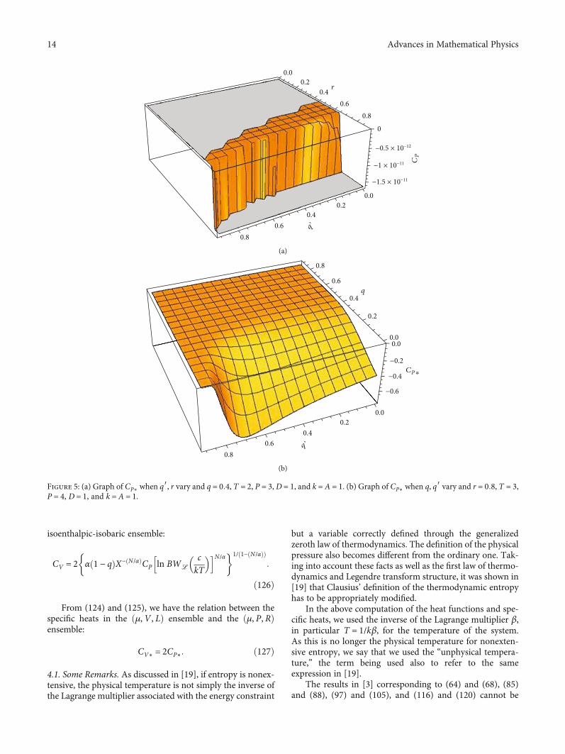
The specific heat at constant pressure is either positive ornegative depending on the values of the deformation param-eters q, q′ and r. For some values of the parameters, the spe-cific heat CP∗ is depicted in Figures 5(a) and 5(b).
12 Advances in Mathematical Physics
4. Relationship among the Specific Heats andSome Remarks
The relationship among the specific heats in the differentensembles is determined as follows. Writing
From (122) and (123), we have the relation between thespecific heats in the microcanonical ensemble and the
q’
0.0
0
−0.5 × 10⁻¹²
−1 × 10⁻¹¹
−1.5 × 10⁻¹¹
0.0
0.2
0.2
0.4
0.4
0.6
0.6
r
Cv
0.8
0.8
(a)
Cv
0.0
0.2
0.2
q
q’0.4
0.4
0.6
0.6
0.8
0.8
−0.6
−0.4
−0.2
0.00.0
(b)
Figure 4: (a) Graph of CV∗ when q′, r vary and q = 0:4,T = 2, P = 3,D = 1, and k = A = 1. (b) Graph of CV∗ when q, q′ vary and r = 0:8, T = 3,P = 4, D = 1, and k = A = 1.
13Advances in Mathematical Physics
isoenthalpic-isobaric ensemble:
CV = 2 α 1 − qð ÞX− N/αð ÞCP ln BWL
ckT
� �h iN/α �1/ 1− N/αð Þð Þ:
ð126Þ
From (124) and (125), we have the relation between thespecific heats in the ðμ, V , LÞ ensemble and the ðμ, P, RÞensemble:
CV∗ = 2CP∗: ð127Þ
4.1. Some Remarks. As discussed in [19], if entropy is nonex-tensive, the physical temperature is not simply the inverse ofthe Lagrange multiplier associated with the energy constraint
but a variable correctly defined through the generalizedzeroth law of thermodynamics. The definition of the physicalpressure also becomes different from the ordinary one. Tak-ing into account these facts as well as the first law of thermo-dynamics and Legendre transform structure, it was shown in[19] that Clausius’ definition of the thermodynamic entropyhas to be appropriately modified.
In the above computation of the heat functions and spe-cific heats, we used the inverse of the Lagrange multiplier β,in particular T = 1/kβ, for the temperature of the system.As this is no longer the physical temperature for nonexten-sive entropy, we say that we used the “unphysical tempera-ture,” the term being used also to refer to the sameexpression in [19].
The results in [3] corresponding to (64) and (68), (85)and (88), (97) and (105), and (116) and (120) cannot be
0
−0.5 × 10⁻¹²
−1 × 10⁻¹¹
−1.5 × 10⁻¹¹
0.0
0.0
0.2
0.2
0.4
0.4
0.6
0.6
r
q’
CP
0.8
0.8
(a)
0.0
0.0
0.0
−0.2
−0.4
−0.6
0.2
0.2
0.4
0.4
0.6
0.6
q
CP
q’
0.8
0.8
⁎
(b)
Figure 5: (a) Graph of CP∗ when q′, r vary and q = 0:4, T = 2, P = 3, D = 1, and k = A = 1. (b) Graph of CP∗ when q, q′ vary and r = 0:8, T = 3,P = 4, D = 1, and k = A = 1.
14 Advances in Mathematical Physics
recovered even when r⟶ 1. The reason is that in the gener-alized statistical mechanics, the thermodynamic limit N⟶∞ and the nonextensive limit q⟶ 1 do not commutewith each other [24, 26]. In the context of the translationalspecific heat, it was observed [24, 26] that the classical q⟶ 1 limit and the thermodynamic limit do not commute.While equations (4.14) and (4.15) of [25] similarly demon-strate that the thermodynamic limit N ⟶∞ of the rota-tional and the diatomic specific heats does not commutewith the corresponding q⟶ 1 classical limits.
5. Conclusion
We have investigated the adiabatic class of ensembles in theframework of generalized mechanics based on the three-parameter entropy. The derivative and branches of the func-tion were in particular useful in the applications to the ther-mostatistics of the nonrelativistic ideal gas. In themicrocanonical ensemble and isoenthalpic-isobaric ensem-ble, the formulas for the three-parameter entropy for an arbi-trary number of particles were obtained. In the large N limit,the heat functions were obtained in terms of the temperatureand expressed in terms of the logarithmic Lambert function.From the heat functions, the specific heats at constant tem-perature were computed. In the ðμ,V , LÞ and the ðμ, P, RÞensembles, an approximate phase volume in the large N limitwas used and the three-parameter entropies of the ensembleswere computed. From the entropy function, the heat func-tion and the specific heat were found and expressed also interms of the logarithmic Lambert function.
Reexamination of the classical gas model using theappropriate expression for the physical temperature will beexplored in a separate paper. The authors, motivated by theapplications of the maximum entropy theory (MaxEnt) inecology [27], also find it interesting to use the q-entropy, ðq, q′Þ-entropy, and ðq, q′, rÞ-entropy to formulate a general-ized maximum entropy theory in ecology.
Data Availability
The computer programs and articles used to generate thegraphs and support the findings of this study are availablefrom the corresponding author upon request.
Conflicts of Interest
The authors declare that they have no conflicts of interest.
Acknowledgments
This research is funded by Cebu Normal University (CNU)and the Philippine Commission on Higher Education-Grants-in-Aid (CHED-GIA) for Research. Thanks are dueto the referees for their comments that led to the improve-ment of the manuscript.
References
[1] B. Zohuri and P. Mcdaniel, “First law of thermodynamics,” inThermodynamics in Nuclear Power Plant SystemsSpringer,Cham.
[2] W. Gibbs, Entropy-Basic Knowledge 101http://www.basicknowledge101.com.
[3] R. Chandrashekar and J. Segar, “Adiabatic thermostatistics ofthe two parameter entropy and the role of Lambert's W-function in its applications,” Physica A, vol. 392, no. 19,pp. 4299–4315, 2013.
[4] S. Asgarani and B. Mirza, “Probability distribution of(Schwammle and Tsallis) two-parameter entropies and theLambert W-function,” Physica A, vol. 387, no. 25, pp. 6277–6283, 2008.
[5] C. G. Chakrabarti and K. De, “Boltzmann-Gibbs entropy: axi-omatic characterization and application,” International Jour-nal of Mathematics and Mathematical Sciences, vol. 23, no. 4,p. 251, 2000.
[6] M. F. Shlesinger, G. M. Zaslavsky, and J. Klafter, “Strangekinetics,” Nature, vol. 363, no. 6424, pp. 31–37, 1993.
[7] C. Beck, “Application of generalized thermostatistics to fullydeveloped turbulence,” Physica A: Statistical Mechanics andits Applications, vol. 277, no. 1-2, pp. 115–123, 2000.
[8] I. Bediaga, E. M. Curado, and J. M. de Miranda, “A nonexten-sive thermodynamical equilibrium approach in e+e−→ had-rons,” Physica A: Statistical Mechanics and its Applications,vol. 286, no. 1-2, pp. 156–163, 2000.
[9] D. B. Walton and J. Rafelski, “Equilibrium distribution ofheavy quarks in Fokker-Planck dynamics,” Physical ReviewLetters, vol. 84, no. 1, pp. 31–34, 2000.
[10] J. Binney and S. Tremaine, Glactic Dynamics, Princeton Uni-versity Press, Princeton, NJ, USA, 1987.
[11] D. C. Clayton, “Maxwellian relative energies and solar neutri-nos,” Nature, vol. 249, no. 5453, p. 131, 1974.
[12] C. Tsallis, “Possible generalization of Boltzmann-Gibbs statis-tics,” Journal of Statistical Physics, vol. 52, no. 1-2, pp. 479–487, 1988.
[13] V. Schẅammle and C. Tsallis, “Two-parameter generalizationof the logarithm and exponential functions and Boltzmann-Gibbs-Shannon entropy,” Journal of Mathematical Physics,vol. 48, no. 11, p. 113301, 2007.
[14] R. Chandrashekar and S. S. N. Mohammed, “A class of energybased ensembles in Tsallis statistics,” Journal of StatisticalMechanics: Theory and Experiment, vol. 2011, no. 5, articleP05018, 2011.
[15] C. B. Corcino and R. B. Corcino, “Three-parameter logarithmand entropy,” Journal of Function Spaces, vol. 2020, Article ID9791789, 10 pages, 2020.
[16] B. Lesche, “Instabilities of Rényi entropies,” Journal of Statisti-cal Physics, vol. 27, no. 2, pp. 419–422, 1982.
[17] G. Kaniadakisa and A. M. Scarfone, “Lesche stability of κ-entropy,” Physica A, vol. 340, no. 1-3, pp. 102–109, 2004.
[18] I. Mező, C. Corcino, and R. Corcino, “Resolution of the plane-symmetric Einstein-Maxwell fields with a generalization of theLambert W function,” Journal of Physics Communications,vol. 4, no. 8, article 085008, 2020.
[19] S. Abe, S. Martinez, F. Pennini, and A. Plastino, “Nonextensivethermodynamic relations,” Physics Letters A, vol. 281, no. 2-3,pp. 126–130, 2001.
[20] F. Reif, Fundamentals of Statistical and Thermal Physics, Inter-national Editions, McGraw-Hill Book Company, Singapore,1985.
[21] D. Ueltschi, “Chapter 1-thermostatics,” 2006, October 2020,http://www.ueltschi.org/teaching/chapthermostatics.pdf.
[22] H. B. Callen, Chapter 8-Thermodynamics and an Introductionto Thermostatistics (2nd Ed.) Statistical Physics Part 1https://www.academia . edu/35013052/Herber t_B_Cal l en_T h e rm o d y n am i c s _ a n d _ a n _ I n t r o d u c t i o n _ t o _Thermostatistics.
[23] R. Gupta, “How to calculate molar heat capacity,” Scien-cinghttps://sciencing.com/calculate-molar-heat-capacity-6184868.html.
[24] S. Abe, “Thermodynamic limit of a classical gas in nonexten-sive statistical mechanics: negative specific heat and polytrop-ism,” Physics Letters A, vol. 263, no. 4-6, pp. 424–429, 1999.
[25] R. Chakrabarti, R. Chandrashekar, and S. S. N. Mohammed,“Rigid rotators and diatomic molecules via Tsallis statistics,”Physica A, vol. 387, no. 18, pp. 4589–4598, 2008.
[26] S. Abe, “Erratum to:“Thermodynamic limit of a classical gas innonextensive statistical mechanics: Negative specific heat andpolytropism”-[Phys. Lett. A 263 (1999) 424-429],” Physics Let-ters A, vol. 267, no. 5-6, pp. 456-457, 2000.
[27] A. B. Brummer and E. A. Newman, “Derivations of the corefunctions of the maximum entropy theory of ecology,”Entropy, vol. 21, no. 7, p. 712, 2019.


![Poincaré Duality for Logarithmic Crystalline Cohomology...structure, this is a generalization of Poincaré duality for crystalline cohomology of a proper smooth scheme ([B] VII).](https://static.documents.pub/doc/80x56/5fc0d14ec7ed06175e361909/poincar-duality-for-logarithmic-crystalline-cohomology-structure-this-is.jpg)


