60
Logistic Regression Analysis Gerrit Rooks 30-03-10
| Date post: | 02-Jan-2016 |
| Category: |
Documents |
| Upload: | aristotle-graves |
| View: | 80 times |
| Download: | 1 times |

Logistic Regression Analysis
Gerrit Rooks30-03-10

This lecture1. Why do we have to know and sometimes use
logistic regression?2. What is the model? What is maximum likelihood
estimation?3. Logistics of logistic regression analysis
1. Estimate coefficients2. Assess model fit3. Interpret coefficients4. Check residuals
4. An SPSS example
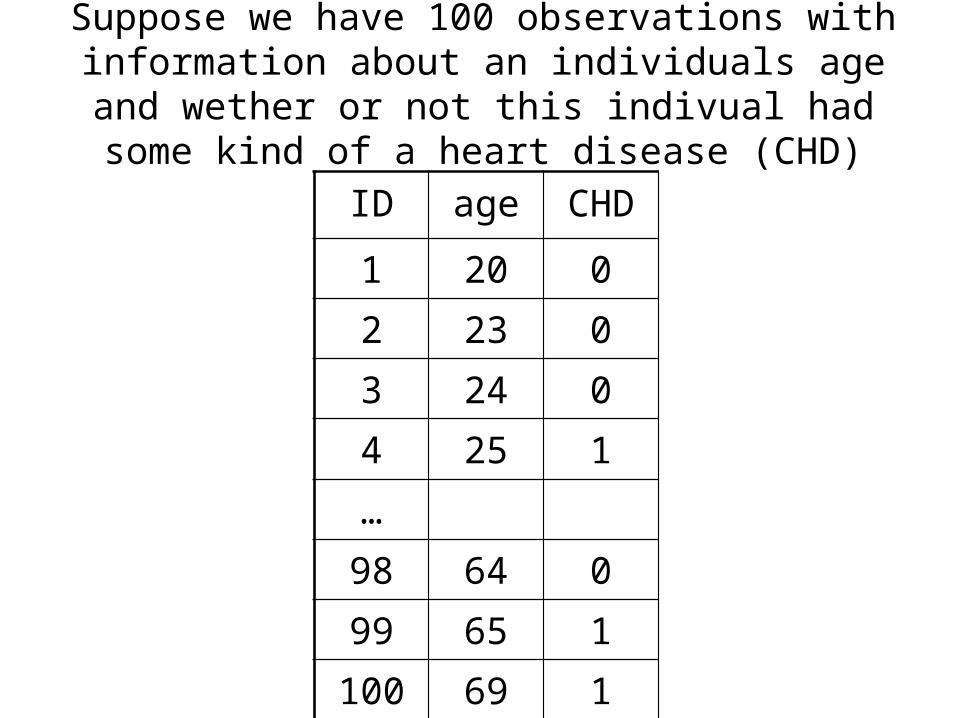
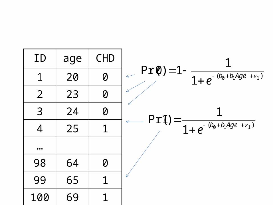
Suppose we have 100 observations with information about an individuals age and wether or not this indivual
had some kind of a heart disease (CHD)
ID age CHD
1 20 02 23 03 24 04 25 1…98 64 099 65 1
100 69 1
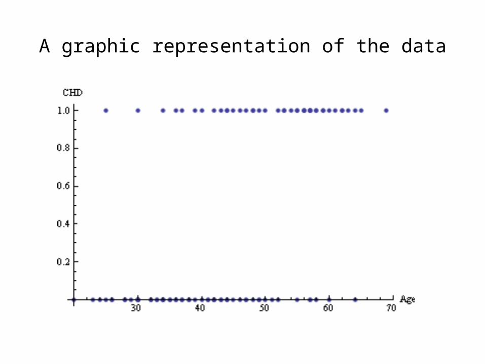
A graphic representation of the data
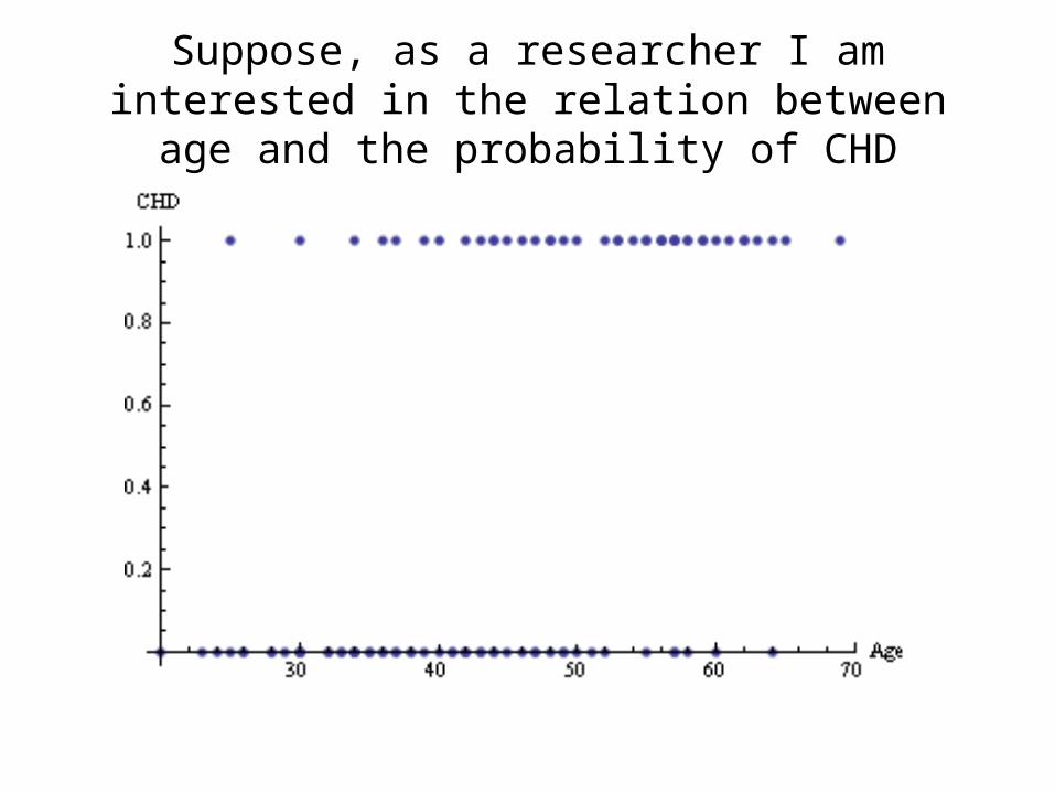
Suppose, as a researcher I am interested in the relation between age and the probability of CHD
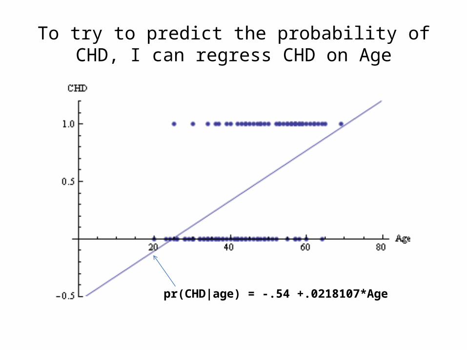
To try to predict the probability of CHD, I can regress CHD on Age
pr(CHD|age) = -.54 +.0218107*Age

However, linear regression is not a suitable model for probalities.
pr(CHD|age) = -.54 +.0218107*Age
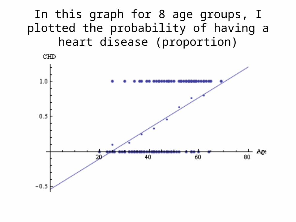
In this graph for 8 age groups, I plotted the probability of having a heart disease (proportion)
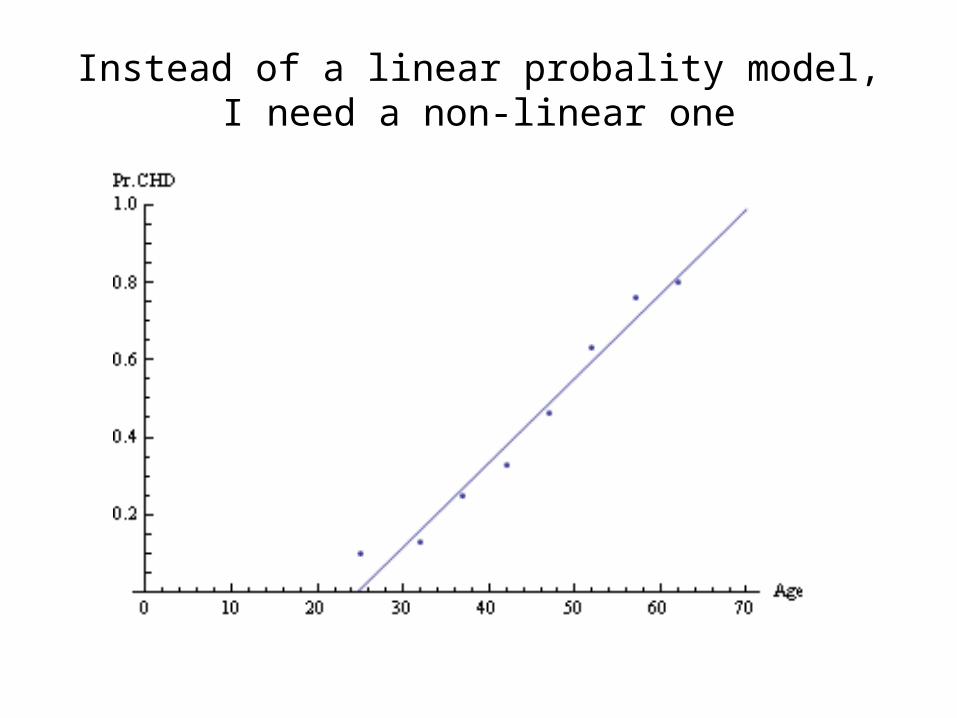
Instead of a linear probality model, I need a non-linear one
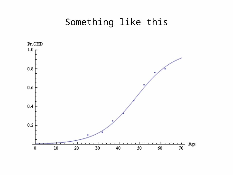
Something like this
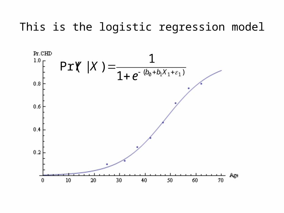
This is the logistic regression model
)( 11101
1)|Pr( Xbbe
XY
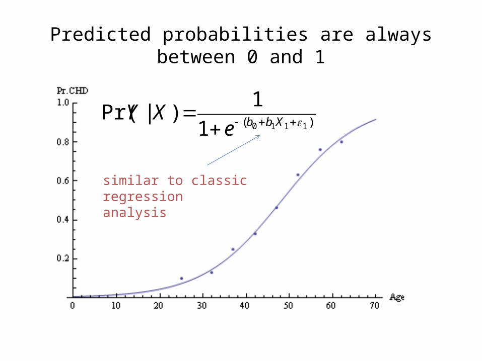
Predicted probabilities are always between 0 and 1
)( 11101
1)|Pr( Xbbe
XY
similar to classic regressionanalysis
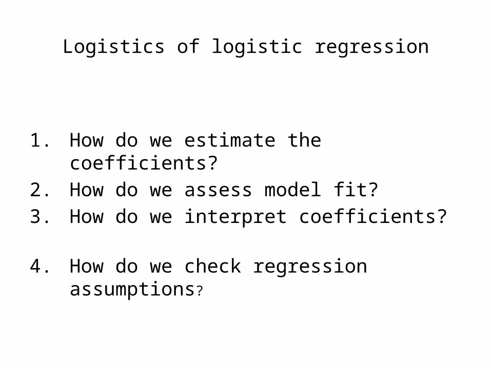
Logistics of logistic regression
1. How do we estimate the coefficients? 2. How do we assess model fit?3. How do we interpret coefficients? 4. How do we check regression assumptions?

Logistics of logistic regression
1. How do we estimate the coefficients? 2. How do we assess model fit?3. How do we interpret coefficients? 4. How do we check regression? assumptions ?

Maximum likelihood estimation
• Method of maximum likelihood yields values for the unknown parameters which maximize the probability of obtaining the observed set of data.
)( 11101
1)|Pr( Xbbe
XY
Unknown parameters

Maximum likelihood estimation
• First we have to construct the likelihood function (probability of obtaining the observed set of data).
Likelihood = pr(obs1)*pr(obs2)*pr(obs3)…*pr(obsn)
Assuming that observations are independent
ID age CHD
1 20 02 23 03 24 04 25 1…98 64 099 65 1
100 69 1
)( 1101
11)0Pr( Agebb
e
)( 1101
1)1Pr( Agebb
e

The likelihood function (for the CHD data)
)1
1(*...
*)1
1(*)
1
11(*
)1
11(*)
1
11(
)(
)()(
)()(
110
110110
110110
Agebb
AgebbAgebb
AgebbAgebb
e
ee
eelikelihood
Given that we have 100 observations I summarize the function
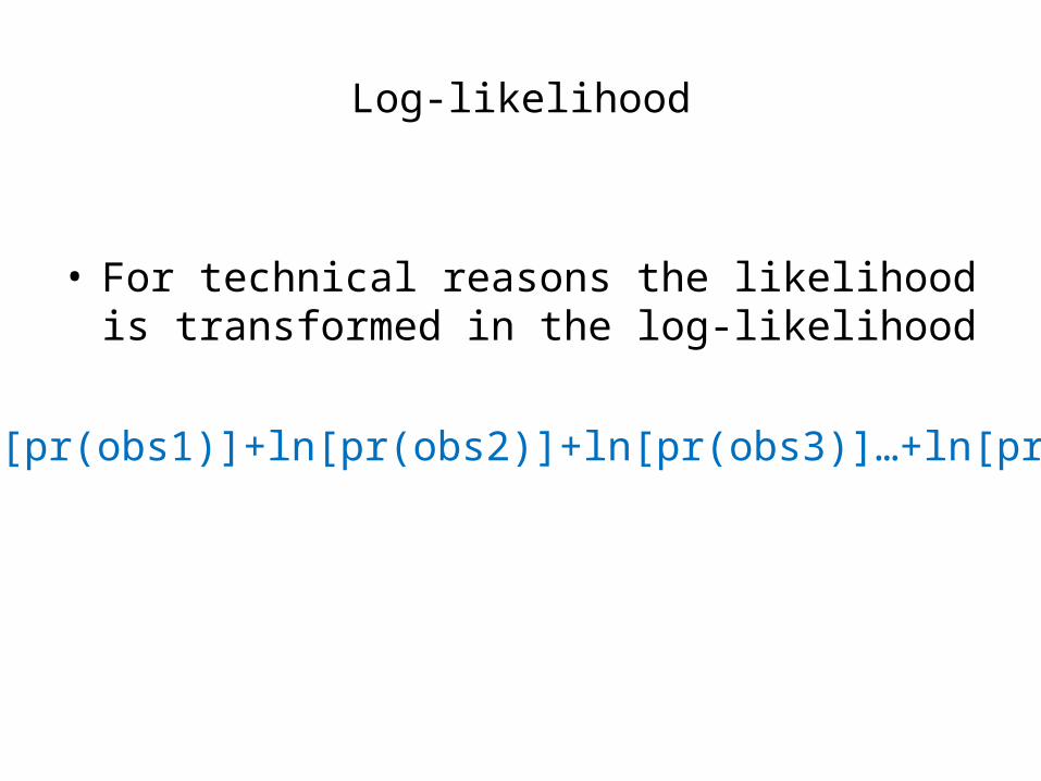
Log-likelihood
• For technical reasons the likelihood is transformed in the log-likelihood
LL= ln[pr(obs1)]+ln[pr(obs2)]+ln[pr(obs3)]…+ln[pr(obsn)]

The likelihood function (for the CHD data)
)1
1(*...
*)1
1(*)
1
11(*
)1
11(*)
1
11(
)(
)()(
)()(
110
110110
110110
Agebb
AgebbAgebb
AgebbAgebb
e
ee
eelikelihood
A clever algorithm gives us values for the parameters b0 and b1 that maximize the likelihood of this data

Estimation of coefficients: SPSS Results
Variables in the Equation
B S.E. Wald df Sig. Exp(B)
Step 1a age ,111 ,024 21,254 1 ,000 1,117
Constant -5,309 1,134 21,935 1 ,000 ,005
a. Variable(s) entered on step 1: age.
)11.3.5( 11
1)|Pr( Xe
XY

)11.3.5( 11
1)|Pr( Xe
XY

)11.3.5( 11
1)|Pr(
XeXY
This function fits very good, other values of b0 and b1 give worse results

Illustration 1: suppose we chose .05X instead of .11X
)05.3.5( 11
1)|Pr( Xe
XY

)40.3.5( 11
1)|Pr(
XeXY
Illustration 2: suppose we chose .40X instead of .11X
Logistics of logistic regression
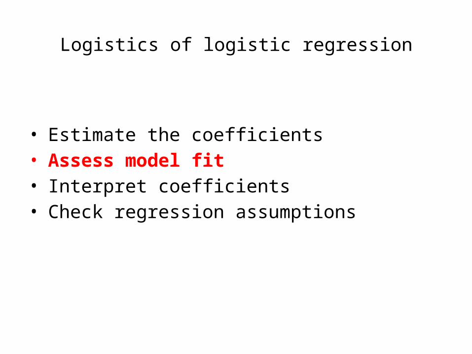
• Estimate the coefficients • Assess model fit• Interpret coefficients • Check regression assumptions

Logistics of logistic regression
• Estimate the coefficients • Assess model fit
– Between model comparisons– Pseudo R2 (similar to multiple regression)– Predictive accuracy
• Interpret coefficients • Check regression assumptions
28
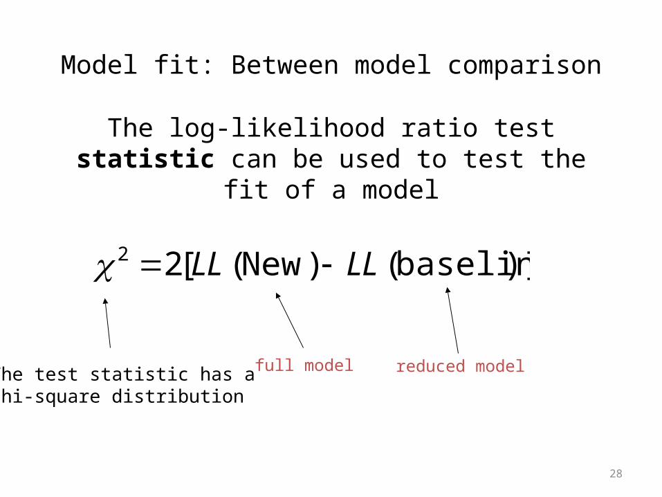
Model fit: Between model comparison
)]baseline()New([22 LLLL
The log-likelihood ratio test statistic can be used to test the fit of a model
The test statistic has achi-square distribution
reduced modelfull model
29
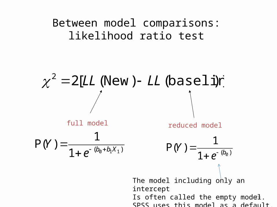
Between model comparisons: likelihood ratio test
)( 1101
1)(P XbbeY
)]baseline()New([22 LLLL
reduced modelfull model
)( 01
1)(P beY
The model including only an interceptIs often called the empty model. SPSS uses this model as a default.

30
Between model comparisons: Test can be used for individual coefficients
)( 221101
1)(P XbXbbeY
)]baseline()New([22 LLLL
reduced modelfull model
)( 01
1)(P beY

)]baseline(2)New(22 LLLL
29.31 = -107,35 – 2LL(baseline)
Omnibus Tests of Model Coefficients
Chi-square df Sig.
Step 1 Step 29,310 1 ,000
Block 29,310 1 ,000
Model 29,310 1 ,000
Model Summary
Step -2 Log likelihood
Cox & Snell R
Square
Nagelkerke R
Square
1 107,353a ,254 ,341
a. Estimation terminated at iteration number 5 because
parameter estimates changed by less than ,001.
-2LL(baseline) = 136,66
This is the test statistic,and it’s associated significance
Between model comparison: SPSS output
32
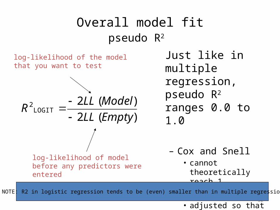
Overall model fitpseudo R2
Just like in multiple regression, pseudo R2 ranges 0.0 to 1.0
– Cox and Snell• cannot theoretically
reach 1
– Nagelkerke• adjusted so that it can
reach 1
)(2
)(2LOGIT
2
EmptyLL
ModelLLR
log-likelihood of modelbefore any predictors wereentered
log-likelihood of the modelthat you want to test
NOTE: R2 in logistic regression tends to be (even) smaller than in multiple regression

33
Overall model fit: Classification table
We correctly predict 74% of our observation
Classification Tablea
Observed
Predicted
chd
0 1
Percentage
Correct
Step 1 chd 0 45 12 78,9
1 14 29 67,4
Overall Percentage 74,0
a. The cut value is ,500

34
Overall model fit: Classification table
14 cases had a CHD while according to our modelthis shouldnt have happened.
Classification Tablea
Observed
Predicted
chd
0 1
Percentage
Correct
Step 1 chd 0 45 12 78,9
1 14 29 67,4
Overall Percentage 74,0
a. The cut value is ,500
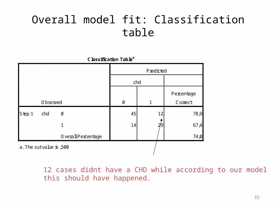
35
Overall model fit: Classification table
12 cases didnt have a CHD while according to our modelthis should have happened.
Classification Tablea
Observed
Predicted
chd
0 1
Percentage
Correct
Step 1 chd 0 45 12 78,9
1 14 29 67,4
Overall Percentage 74,0
a. The cut value is ,500

Logistics of logistic regression
• Estimate the coefficients • Assess model fit• Interpret coefficients • Check regression assumptions

Logistics of logistic regression
• Estimate the coefficients • Assess model fit• Interpret coefficients
– Direction– Significance– Magnitude
• Check regression assumptions
38
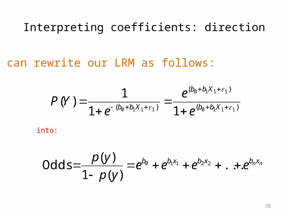
Interpreting coefficients: direction
)(
)(
)( 1110
1110
1110 11
1)(
Xbb
Xbb
Xbb e
e
eYP
We can rewrite our LRM as follows:
into:
nnxbxbxbb eeeeyp
yp
...
)(1
)(Odds 22110

39
Interpreting coefficients: direction
• original b reflects changes in logit: b>0 -> positive relationship
• exponentiated b reflects the changes in odds: exp(b) > 1 -> positive relationship
nnxbxbxbbyp
yp
...
)(1
)(lnlogit 22110
nnxbxbxbb eeeeyp
yp
...
)(1
)(Odds 22110
40
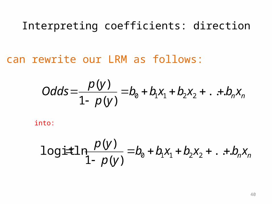
Interpreting coefficients: direction
We can rewrite our LRM as follows:
into:
nnxbxbxbbyp
yp
...
)(1
)(lnlogit 22110
nnxbxbxbbyp
ypOdds
...
)(1
)(22110

41
Interpreting coefficients: direction
• original b reflects changes in logit: b>0 -> positive relationship
• exponentiated b reflects the changes in odds: exp(b) > 1 -> positive relationship
nnxbxbxbbyp
yp
...
)(1
)(lnlogit 22110
nnxbxbxbb eeeeyp
yp
...
)(1
)(Odds 22110

42
Testing significance of coefficients
• In linear regression analysis this statistic is used to test significance
• In logistic regression something similar exists
• however, when b is large, standard error tends to become inflated, hence underestimation (Type II errors are more likely)
b
b
SEWald
t-distribution standard error of estimate
estimate
Note: This is not the Wald Statistic SPSS presents!!!

Interpreting coefficients: significance
• SPSS presents
• While Andy Field thinks SPSS presents this:
bSE
b2
2
Wald
b
b
SEWald

44
3. Interpreting coefficients: magnitude
• The slope coefficient (b) is interpreted as the rate of change in the "log odds" as X changes … not very useful.
• exp(b) is the effect of the independent variable on the odds, more useful for calculating the size of an effect
nnxbxbxbbyp
yp
...
)(1
)(lnlogit 22110
nnxbxbxbb eeeeyp
yp
...
)(1
)(Odds 22110

Magnitude of association: Percentage change in odds
• (Exponentiated coefficienti - 1.0) * 100
event
event
prob1
probOddsi
Probability Odds
25% 0.33
50% 1
75% 3

Variables in the Equation
B S.E. Wald df Sig. Exp(B)
Step 1a age ,111 ,024 21,254 1 ,000 1,117
Constant -5,309 1,134 21,935 1 ,000 ,005
a. Variable(s) entered on step 1: age.
46
• For our age variable:– Percentage change in odds = (exponentiated coefficient – 1) * 100 = 12%– A one unit increase in previous will result in 12% increase in the odds that
the person will have a CHD– So if a soccer player is one year older, the odds that (s)he will have CHD is
12% higher
Magnitude of association

Another way: Calculating predicted probabilities
)11.3.5( 11
1)|Pr(
XeXY
So, for somebody 20 years old, the predicted probability is .04
For somebody 70 years old, the predicted probability is .91
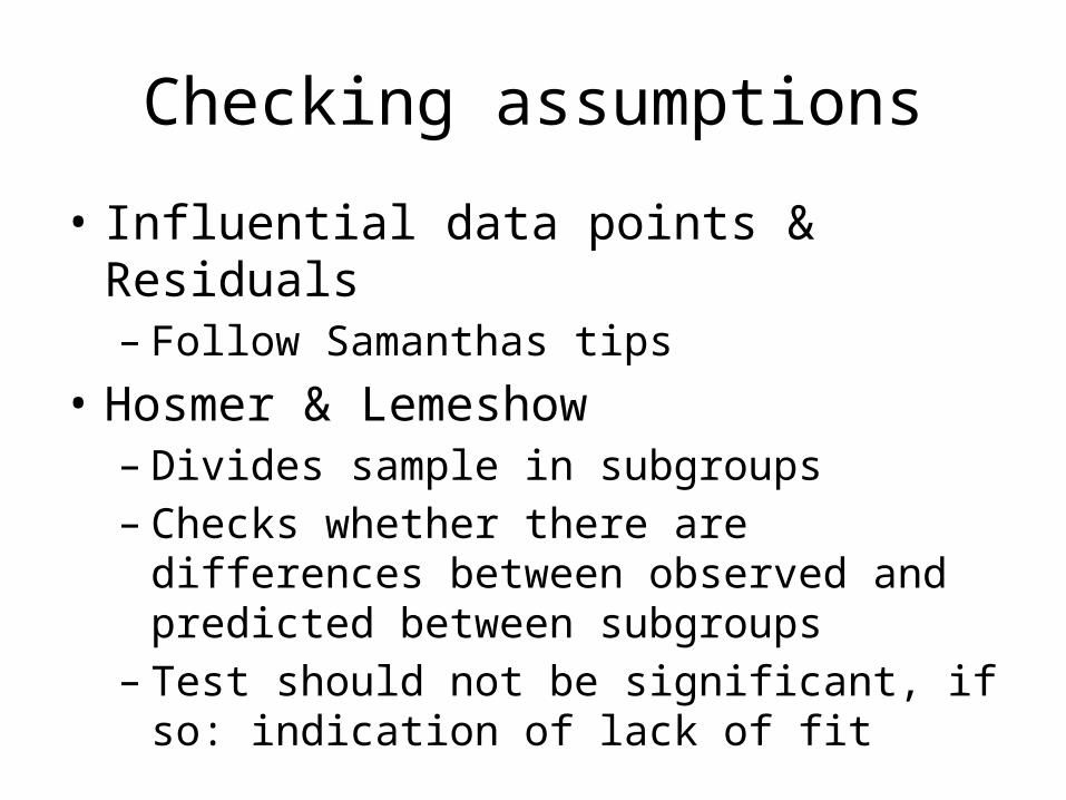
Checking assumptions
• Influential data points & Residuals– Follow Samanthas tips
• Hosmer & Lemeshow– Divides sample in subgroups– Checks whether there are differences between
observed and predicted between subgroups– Test should not be significant, if so: indication of
lack of fit

Hosmer & Lemeshow
Test divides sample in subgroups, checks whether difference between observed and predicted is about equal in these groups
Test should not be significant (indicating no difference)

Examining residuals in lR
1. Isolate points for which the model fits poorly2. Isolate influential data points

Residual statistics
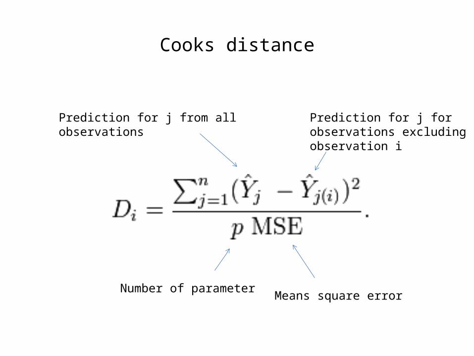
Cooks distance
Means square errorNumber of parameter
Prediction for j from all observations
Prediction for j for observations excludingobservation i

53
Illustration with SPSS
• Penalty kicks data, variables:– Scored: outcome variable,
• 0 = penalty missed, and 1 = penalty scored
– Pswq: degree to which a player worries– Previous: percentage of penalties scored by a
particulare player in their career

54
Case Processing Summary
75 100,0
0 ,0
75 100,0
0 ,0
75 100,0
Unweighted Casesa
Included in Analysis
Missing Cases
Total
Selected Cases
Unselected Cases
Total
N Percent
If weight is in effect, see classification table for the totalnumber of cases.
a.
Dependent Variable Encoding
0
1
Original ValueMissed Penalty
Scored Penalty
Internal Value
SPSS OUTPUT Logistic Regression
Tells you somethingabout the number of observations and missings

55
Classification Tablea,b
0 35 ,0
0 40 100,0
53,3
ObservedMissed Penalty
Scored Penalty
Result of PenaltyKick
Overall Percentage
Step 0
MissedPenalty
ScoredPenalty
Result of Penalty Kick
PercentageCorrect
Predicted
Constant is included in the model.a.
The cut value is ,500b.
Variables in the Equation
,134 ,231 ,333 1 ,564 1,143ConstantStep 0B S.E. Wald df Sig. Exp(B)
Variables not in the Equation
34,109 1 ,000
34,193 1 ,000
41,558 2 ,000
previous
pswq
Variables
Overall Statistics
Step0
Score df Sig.
Block 0: Beginning Blockthis table is based on the empty model, i.e. onlythe constant in the model
)( 01
1)(P beY
these variableswill be enteredin the modellater on

56
Block 1: Method = Enter
Omnibus Tests of Model Coefficients
54,977 2 ,000
54,977 2 ,000
54,977 2 ,000
Step
Block
Model
Step 1Chi-square df Sig.
Model Summary
48,662a ,520 ,694Step1
-2 Loglikelihood
Cox & SnellR Square
NagelkerkeR Square
Estimation terminated at iteration number 6 becauseparameter estimates changed by less than ,001.
a.
)]baseline()New([22 LLLL
Block is useful to check significance of individual coefficients, see Field
New model
this is the test statistic
after dividing by -2
Note: Nagelkerkeis larger than Cox

57
Variables in the Equation
,065 ,022 8,609 1 ,003 1,067
-,230 ,080 8,309 1 ,004 ,794
1,280 1,670 ,588 1 ,443 3,598
previous
pswq
Constant
Step1
a
B S.E. Wald df Sig. Exp(B)
Variable(s) entered on step 1: previous, pswq.a.
Classification Tablea
30 5 85,7
7 33 82,5
84,0
ObservedMissed Penalty
Scored Penalty
Result of PenaltyKick
Overall Percentage
Step 1
MissedPenalty
ScoredPenalty
Result of Penalty Kick
PercentageCorrect
Predicted
The cut value is ,500a.
Block 1: Method = Enter (Continued)
Predictive accuracy has improved (was 53%)
estimatesstandard errorestimates
significance based on Wald statistic
change in odds
58
Variables in the Equation
,065 ,022 8,609 1 ,003 1,067
-,230 ,080 8,309 1 ,004 ,794
1,280 1,670 ,588 1 ,443 3,598
previous
pswq
Constant
Step1
a
B S.E. Wald df Sig. Exp(B)
Variable(s) entered on step 1: previous, pswq.a.
Classification Tablea
30 5 85,7
7 33 82,5
84,0
ObservedMissed Penalty
Scored Penalty
Result of PenaltyKick
Overall Percentage
Step 1
MissedPenalty
ScoredPenalty
Result of Penalty Kick
PercentageCorrect
Predicted
The cut value is ,500a.
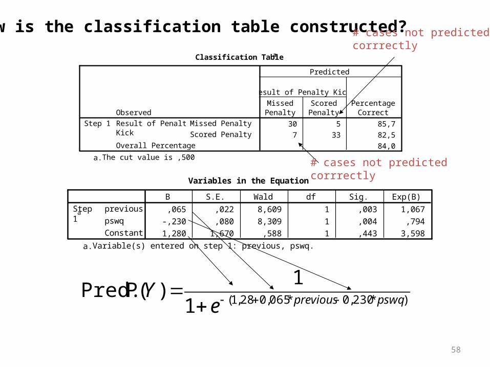
How is the classification table constructed?
)*230,0*065,028,1(1
1)(P Pred.
pswqpreviouseY
# cases not predictedcorrrectly
# cases not predictedcorrrectly

59
How is the classification table constructed?
)*230,0*065,028,1(1
1)(P Pred.
pswqpreviouseY
pswq previous scored Predict. prob.
18 56 1 .68
17 35 1 .41
20 45 0 .40
10 42 0 .85
60
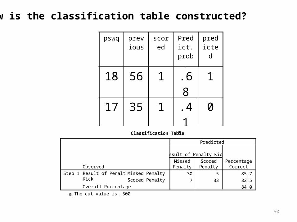
How is the classification table constructed?
pswq previous
scored Predict. prob.
predicted
18 56 1 .68 1
17 35 1 .41 0
20 45 0 .40 0
10 42 0 .85 1
Classification Tablea
30 5 85,7
7 33 82,5
84,0
ObservedMissed Penalty
Scored Penalty
Result of PenaltyKick
Overall Percentage
Step 1
MissedPenalty
ScoredPenalty
Result of Penalty Kick
PercentageCorrect
Predicted
The cut value is ,500a.


