42
1 270J/ESD 273J 1.270J/ESD.273J L Logi isti tics and Di d Dist trib ibuti tion S Syst tems Dynamic Economic Lot Sizing Model 1
| Date post: | 07-Sep-2018 |
| Category: |
Documents |
| Upload: | doannguyet |
| View: | 213 times |
| Download: | 0 times |

1 270J/ESD 273J1.270J/ESD.273J
LLogiistitics and Di d Disttribibutition SSysttems
Dynamic Economic Lot Sizing Model
1

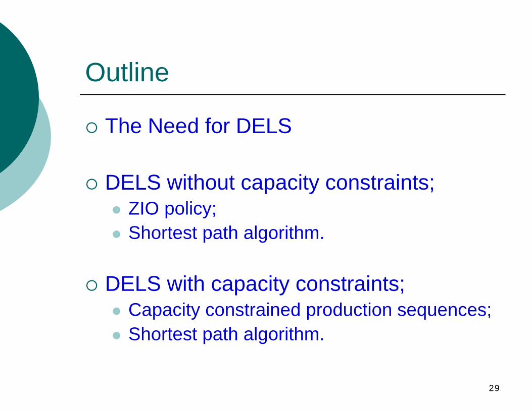
Outline
{ The Need for DELS
{ DELS without capacity constraints: z ZIO policy; ZIO policy;z Shortest path algorithm.
{ DELS with capacity constraints: z C it t i d dCapacity constrained producti tion sequences; z Shortest path algorithm.
2

Strategic Sourcing Inputs
Transportation costs, rules for shipping out of
territory overflowSupplier
WH cost, capacity, safety stock targets, and current on hand territory overflow
facilitiesconstraints, costs, fixed orders, etc
and current on-hand position
Mfg constraints, costs, run rules, fixed production
schedules set ups tooling etcCurrent demand
forecast by forecast Product info and
BOM
3
schedules, set-ups, tooling, etc. by time period
ylocation by time period
BOM

Key Drivers in Sourcing Decisions
� Freight costs for existing and potential lanes
� Availability at different times of the year
Freight Production
Raw Materials �
p � Duties for different
customer countries
g & Duties Capabilities �
Locations Mfg Costs
Sourcing Decisions
� Suppliers � Plants � Warehouses
Costs� Customers
Products Demand � Demand by product
by customer� Product attributes � BOM information
� Purchase prices
What can be made where, tooling, etc. MfMfg speedds && capacities
� Setups, batches, yield loss, etc.
� Production costs � Allocation of fixed & Allocation of fixed &
variable overheads � Economies of scale
� BOM information � Special rules and
� Monthly or weekly forecasts
constraints
4
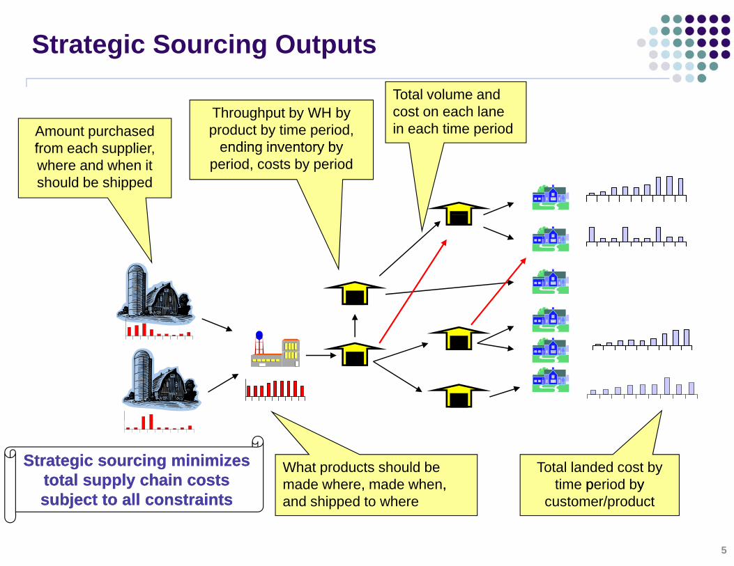
Strategic Sourcing Outputs
Total volume and cost on each lane in each time periodAmount purchased
from each supplier
Throughput by WH by product by time period,
ending inventory byfrom each supplier, where and when it should be shipped
ending inventory by period, costs by period
What products should be made where, made when,
Total landed cost by time period by
Strategic sourcing minimizesStrategic sourcing minimizestotal supply chain coststotal supply chain costs
5
, ,and shipped to where
p ycustomer/productsubject to all constraintssubject to all constraints
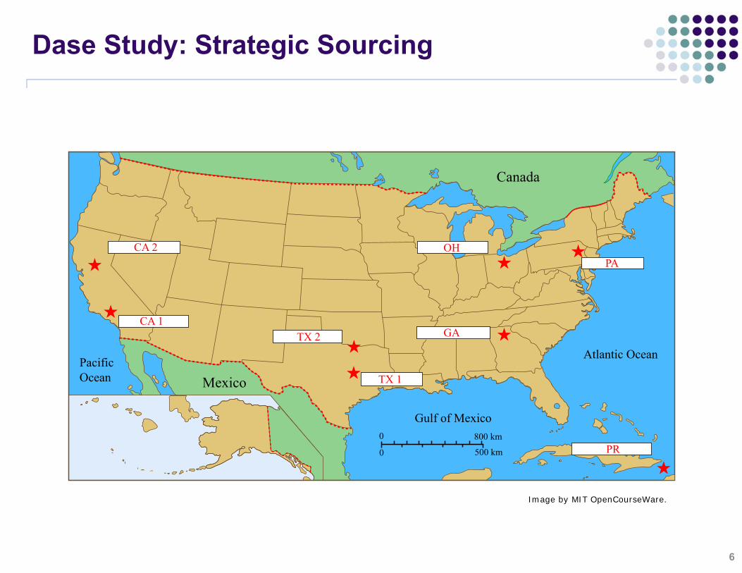
ICI LOCATIONSDase Study: Strategic Sourcing
PR
6
Gulf of Mexico
Atlantic OceanPacific Ocean
0
0
800 km
500 km
CA 2
CA 1TX 2
TX 1
GA
OHPA
PR
Mexico
Canada
Image by MIT OpenCourseWare.
�
Background
� Sold product throughout US to variety of customers z Direct to customers/distributors z Direct to customers/distributors z Through their own stores z Through retailers
� Wide variety of product z 4,000 different SKU’s z 1500 different base products (could be labeled differently) z Many low-volume products
� Batch ManufacturingM f t i d i b t h th i ifi t i f l if z Manufacturing done in batch, so there significant economies of scale if a single product is made in one location
� Mfg Capability Mfg Capability z Each plant had many different processes z Many plants can produce the same problem
7
Business Problems
� Are products being made in the right location?
� Should plants produce a lot of products to serve the local market or should a plant produce a few products tomarket or should a plant produce a few products tominimize production costs?
� Should we close the high cost plant?
� HHow shhould we manage all th ll the llow vollume SKU’s??ld SKU’
8

Key Driver - Data Collection
Raw Material Costs•Invoice cost
Variable Mfg. Costs•Variable Mfg costs by process/by site•Invoice cost
•Freight cost•% shrinkage•Difficulty - Medium
•Variable Mfg. costs by process/by site•Difficulty - High
Technical Capability Manufacturing Capability
Key Driversp y
•Product Family•Difficulty - High
Manufacturing Capability•Demonstrated Capacity•Difficulty - High
Interplant Freight CostsYield Loss Interplant Freight Costs•Average run rates in from site to site•Difficulty - Low
Yield Loss•% of lost volume per 100 units•Site Specific•Difficulty - Low
9

Process Change
Existing Process New Process
Sourcing decisions currently made in isolationDecisions are made for small groups of products
Sourcing decisions made in context of entire supply chain
Decisions are made considering the entire supply chain
Excel is the primary decision tool – Many drawbacksExcel does not capture the many different trade-offs that exist in the supply chainE l l l l t th t f i
supply chain
Sourcing decisions are made using Master PlanningOptimization model provides global optimization capability
Excel can only calculate the costs for a given decision; it cannot make decisions
No formal data collection processData not collected systematically across the
Model automatically updates for on-going decision making
Developed process for automatically updating and maintaining the model so the decisionsData not collected systematically across the
supply chain to make these decisionsand maintaining the model so the decisions can be made on an on-going basis
Built 2 Models1. Model for all the base products2 Model for low volume SKU’s
10
2. Model for low volume SKU s
�
z
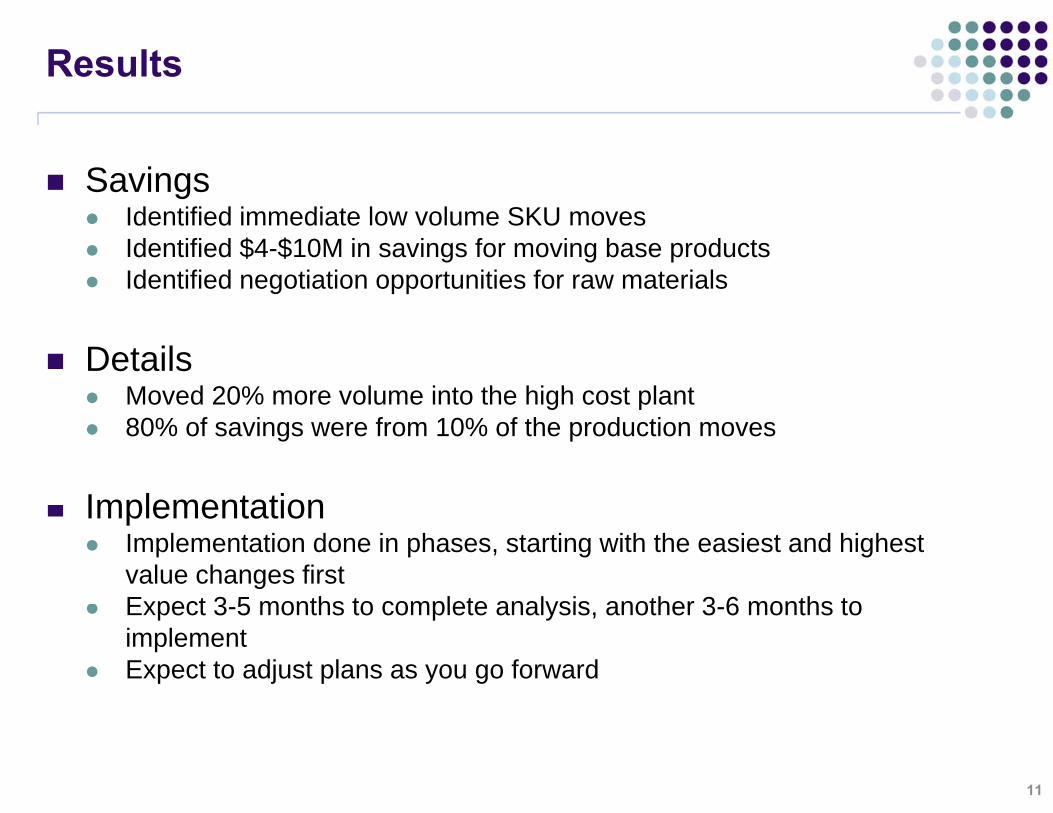
Results
� Savings Id tifi d i di t l l SKUz Identified immediate low volume SKU moves
z Identified $4-$10M in savings for moving base products z Identified negotiation opportunities for raw materials
� Details z Moved 20% more volume into the high cost plantg p z 80% of savings were from 10% of the production moves
� ImplementationImplementation z Implementation done in phases, starting with the easiest and highest
value changes first Expect 3 5 months to complete analysis another 3 6 months to z Expect 3-5 months to complete analysis, another 3-6 months to implement
z Expect to adjust plans as you go forward
11

More Volume to High Cost Plant
� Baseline P d t A 20% f th l 45% f th i bl tz Product A: 20% of the volume, 45% of the variable cost
z Product B: 80% of the volume, 55% of the variable cost
� O ti i ti Optimization z Product A: 5% of the volume, 15% of the variable cost z Product B: 95% of the volume, 85% of the variable cost
� Net change was an increase in total volume
12

Case Study 3: Optimizing S&OP at PBG
M k S ll D li S iMake Sell Deliver Service
PBG Operates 57 Plants in the U.S. and 103 Plants Worldwide
Over 125 Million 8 oz. Servings are Enjoyed by Pepsi Customers
240,000 Miles are Logged Every Day to Meet the Needs of Our Customers
Strong Customer Service Culture Identified as “Customer p
Each Day!Our Customers
Connect”

PBG Structure - The PBG Territory
{PBG accounts for 58% of the domestic Pepsi Volume…the other 42% is {generated through a network of 96 Bottlers g g
{Each BUs act independently and meet local needs
Southeast
Atlantic
Central
Great West
WestAK
CA
NV
OR
WA
ID
MT ND
SDMN
WI
IL
MI
IN
KY
TN
AL GA
ME
NHVT
NY
PA
VA
NC
WV
OH
SC
CTMA
RI
NJ
DEMD
FL
MS
IA
MO
AR
LA
NE
KS
OK
TX
WY
UT
AZ NM
CO
Central
Atlantic
Southeast
Great West
West
Image by MIT OpenCourseWare.

Challenges and Objective
� Problem: How should the firm source its products to minimize cost and maximize availability?minimize cost and maximize availability?
� Objjective: Determine where pproducts should be pproduced to reduce overall supply chain costs and meet all relevant business constraints
15 ©Copyright 2008 D.
Simchi-Levi

Optimization Basics
Tradeoffs associated with optimizing a network…
©Copyright 2008 D. Simchi-Levi
16
Would like to maximize the number of products produced at a location to minimize transportation costs
Hi h t High cost plants may be close to key markets
Would like to minimize the number of products produced at a location to maximize product run size
Capacity Constraints
Image by MIT OpenCourseWare.

Optimization Scenario
Optimized Central BU model:
Total Cost
Category Baseline Optimized Difference % savingsMFG Cost 2,610,361.00$ 2,596,039.00$ 14,322.00$ 0.6%Trans Cost 934,920.00$ 857,829.00$ 77,091.00$ 9.0%Total Cost 3 545 281 00$ 3 453 868 00$ 91 413 00$ 2 6%Total Cost 3,545,281.00$ 3,453,868.00$ 91,413.00$ 2.6%
Production Breakdown
Plant Baseline Optimized % changeBurnsville 2 444 277 00 2 457 688 00 1%
Units Produced
Burnsville 2,444,277.00 2,457,688.00 1%Howell 3,509,708.00 3,828,727.50 8%Detroit 2,637,253.00 2,304,822.50 -14%
©Copyright 2008 D. Simchi-Levi 17
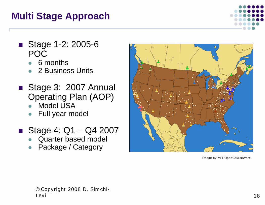
Multi Stage Approach
Stage 1-2: 2005-6 POCPOC
6 months2 Business Units
Stage 3: 2007 Annual Operating Plan (AOP)
Model USAFull year model
St 4 Q1 Q4 2007Stage 4: Q1 – Q4 2007Quarter based modelPackage / Category
©Copyright 2008 D. Simchi-Levi 18
Image by MIT OpenCourseWare.

- -
Impact
� Creation of regular meetings bringing together Supply chain, Transport, Finance, Sales and Manufacturing functions to discuss sourcing and pre-build strategies
� Reduction in raw material and supplies inventory from $201 to $195 millionto $195 million
� A 2 percentage point decline in in growth of transport miles even as revenue greweven as revenue grew
� An additional 12.3 million cases available to be sold due to reduction in warehouse out-of-stock levels
To put the last result in perspective the reduction in warehouse out-of-stock levels To put the last result in perspective, the reduction in warehouse out of stock levels effectively added one and a half production lines worth of capacity to the firm’s supply chain without any capital expenditure.
19
Outline
{ The Need for DELS
{ DELS without capacity constraints: z ZIO policy; ZIO policy;z Shortest path algorithm.
{ DELS with capacity constraints: z C it t i d dCapacity constrained producti tion sequences; z Shortest path algorithm.
20

Assumptions
{ Finite horizon: T periods; { Varying demands: d t=1 T; { Varying demands: dt, t=1,…,T; { Linear ordering cost: Ktδ(yt)+ctyt ; { Linear holding cost: ht ; { Inventoryy level at the end of pperiod t,, I tt
{ No shortage; {{ Zero lead time;Zero lead time; { Sequence of Events: Review, Place Order,
O d A i D d i R li dOrder Arrives, Demand is Realized 21

Wagner-Whitin (W-W) Model
22
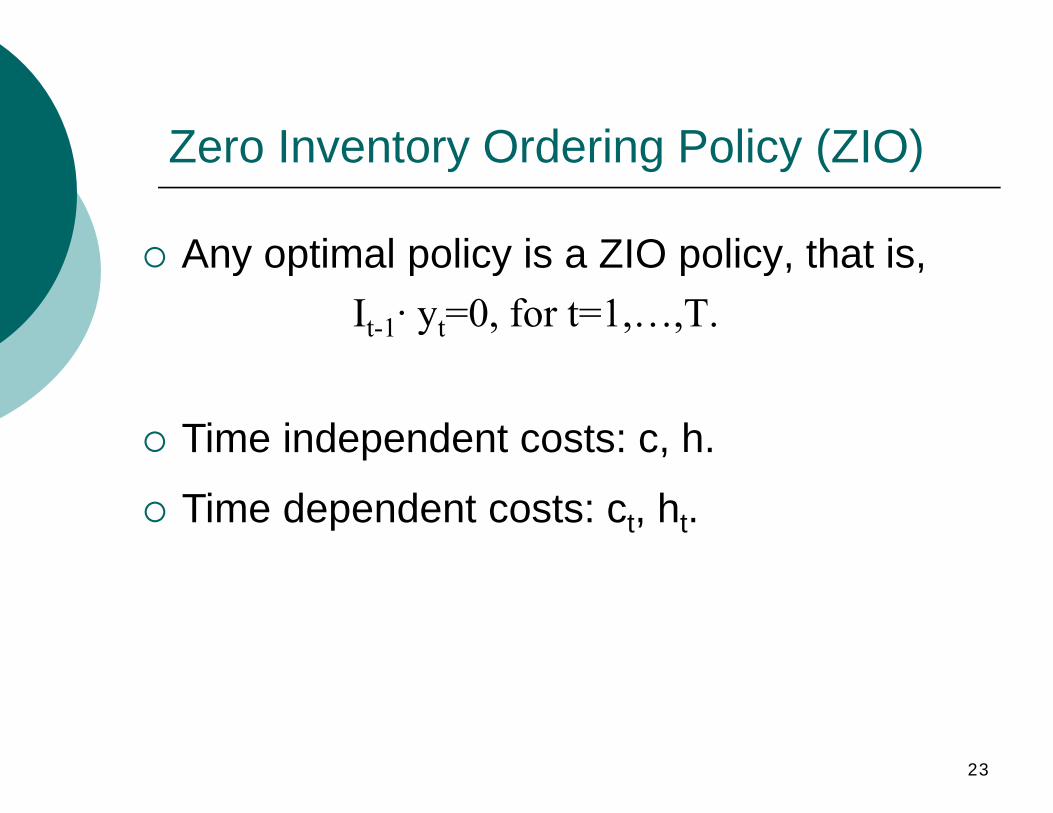
Zero Inventory Ordering Policy (ZIO)
{ Any optimal policy is a ZIO policy, that is,I y 0 for t 1 TIt-1· yt=0, for t=1,…,T.
{ Time independent costs: c, h.
{ Time dependent costs: c { Time dependent costs: ct, hht.
23
-
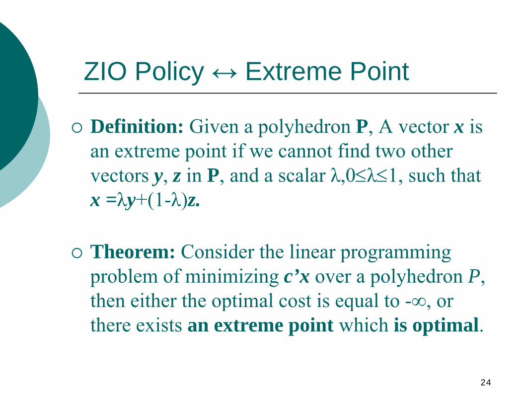
ZIO Policy ↔ Extreme Point
{ Definition: Given a polyhedron P, A vector x is an extreme point if we cannot find two otheran extreme point if we cannot find two other vectors y, z in P, and a scalar λ,0≤λ≤1, such that x =λy+(1-λ)zx λy+(1 λ)z.
{ Theorem: Consider the linear programming { Theorem: Consider the linear programming problem of minimizing c’x over a polyhedron P, then either the optimal cost is equal to then either the optimal cost is equal to -∞∞, oror there exists an extreme point which is optimal.
24

Min-Cost Flow Problem
S
y1 yT
21 t TT-1
y y y1 t T yt
It-1
dTd1 dt
25
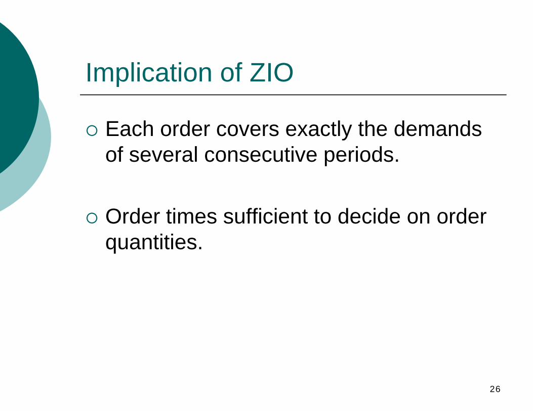
Implication of ZIO
{ Each order covers exactly the demands of several consecutive periodsof several consecutive periods.
{ Order times sufficient to decide on order quantities.
26
⎪
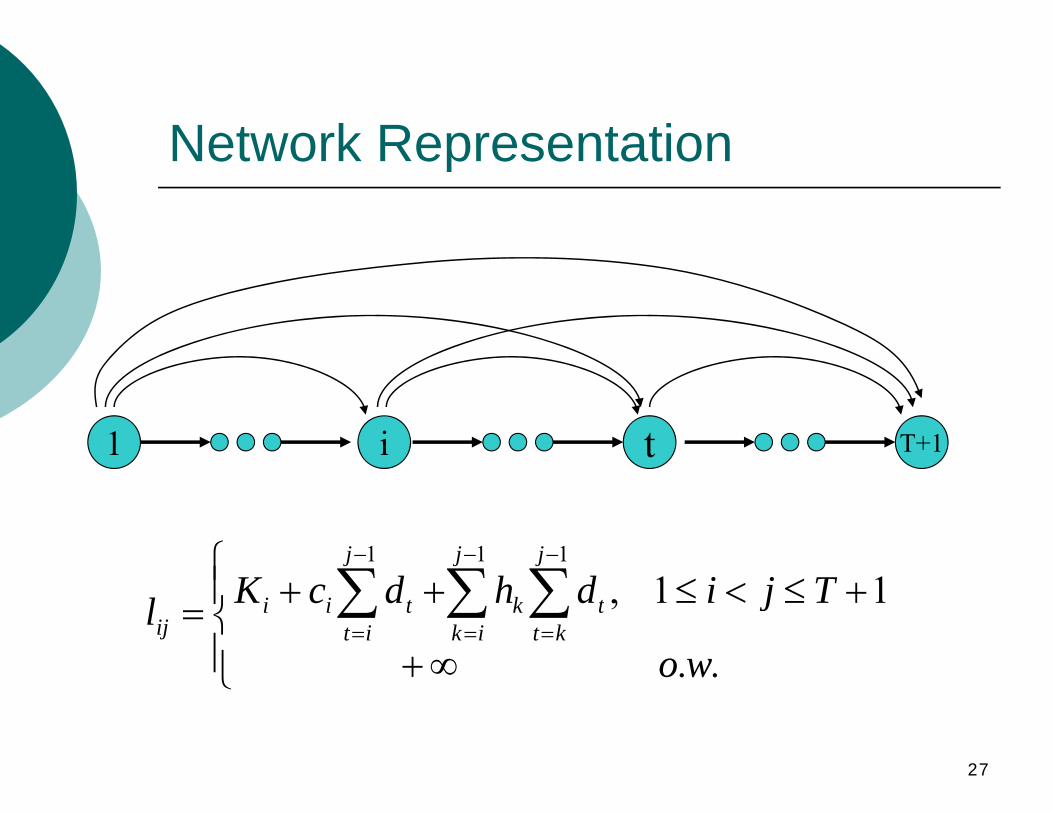
Network Representation
i1 T+1t
⎧ j−1 j−1 j−1
⎪Kii + cii ∑∑ dtt +∑∑ hkk ∑∑ dtt ,, 1 ≤ i < jj ≤ T +1l =lij ⎨⎨ t=i k =i t=k⎪⎩ +∞ o.w.
27
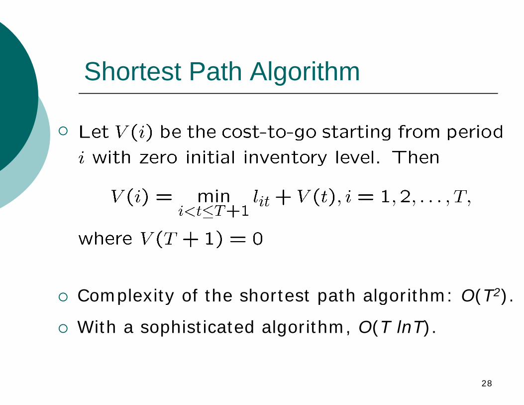
Shortest Path Algorithm
{
{ Complexity of the shortest path algorithm: O(T2).).{ Complexity of the shortest path algorithm: O(T
{ With a sophisticated algorithm, O(T lnT).
28
Outline
{ The Need for DELS
{ DELS without capacity constraints; z ZIO policy; ZIO policy;z Shortest path algorithm.
{ DELS with capacity constraints; z C it t i d dCapacity constrained producti tion sequences; z Shortest path algorithm.
29

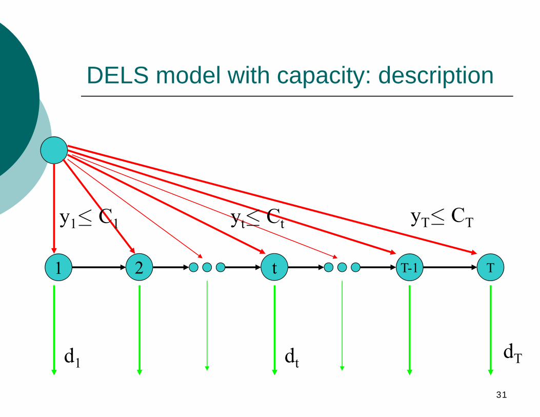
DELS with Capacity Constraints
30
≤
DELS model with capacity: description
21 t
y1≤ C1 yT≤ CCTyt≤ Ct
TT-1
d dTT d11 dt dt
31
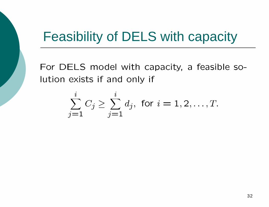
Feasibility of DELS with capacity
32

Inventory Decomposition Property
33
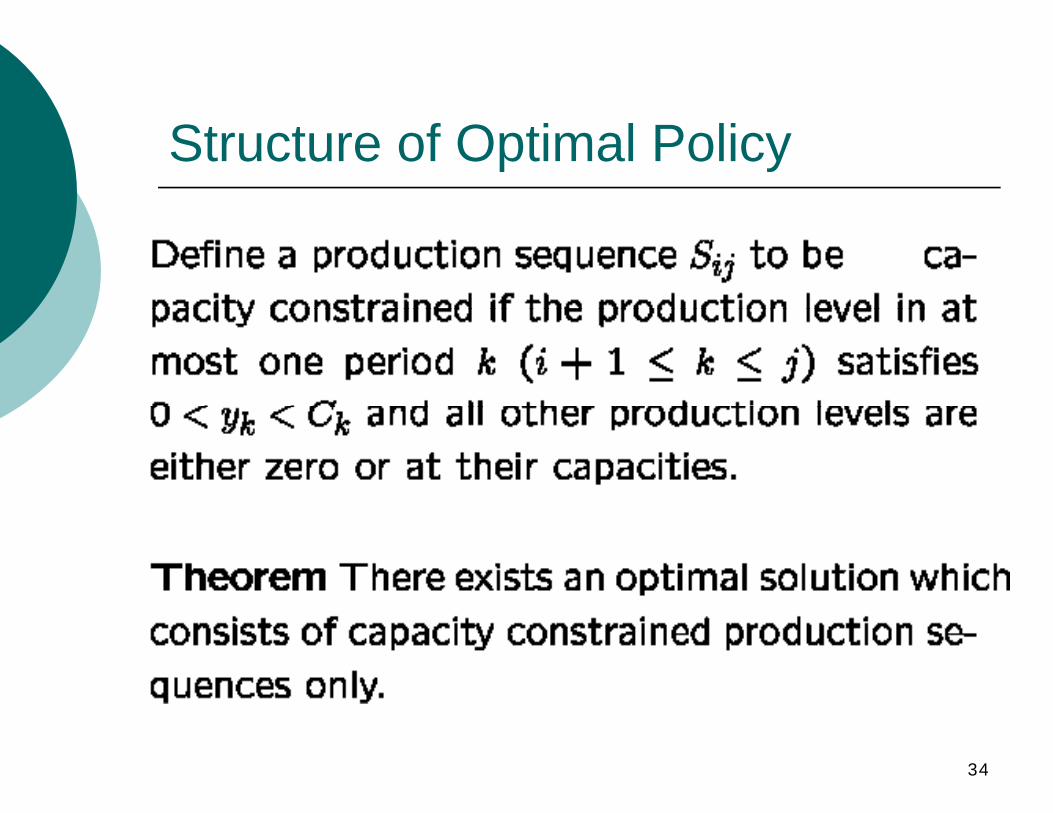
Structure of Optimal Policy
34
≤
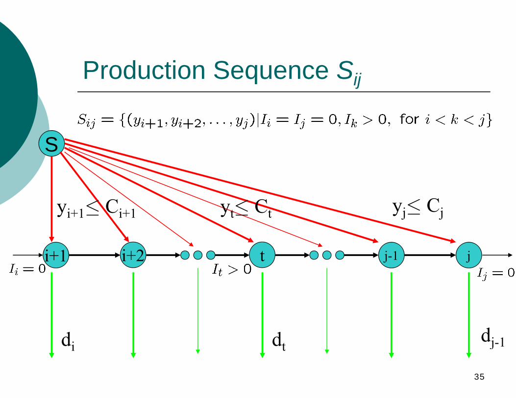
Production Sequence Sij
SS
C yi+1≤ Ci+1 yt≤ Ct yj≤ Cj
i+2i+1 t jj-1
di dt dj-1di dt j 1
35
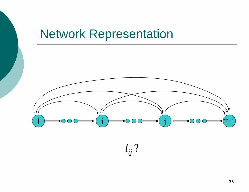
Network Representation
i1 T 1ji1 T+1j
lij ?
36
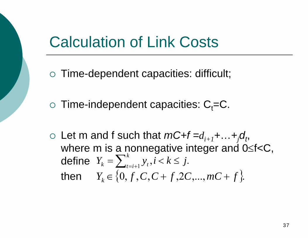
Calculation of Link Costs
{ Time-dependent capacities: difficult;
{ Time-independent capacities: Ct=C.
{ Let m and f such that mC+f =di+1+…+jdt, where m is a nonnegative integer and 0≤f<Cwhere m is a nonnegative integer and 0≤f<C, define Yk =∑t
k
=i+1 yt , i < k ≤ j.
then YYk ∈{0 ff ,C,C ++ f C,..., mC + f }then ∈{0, C C f ,22C mC + f }.
37
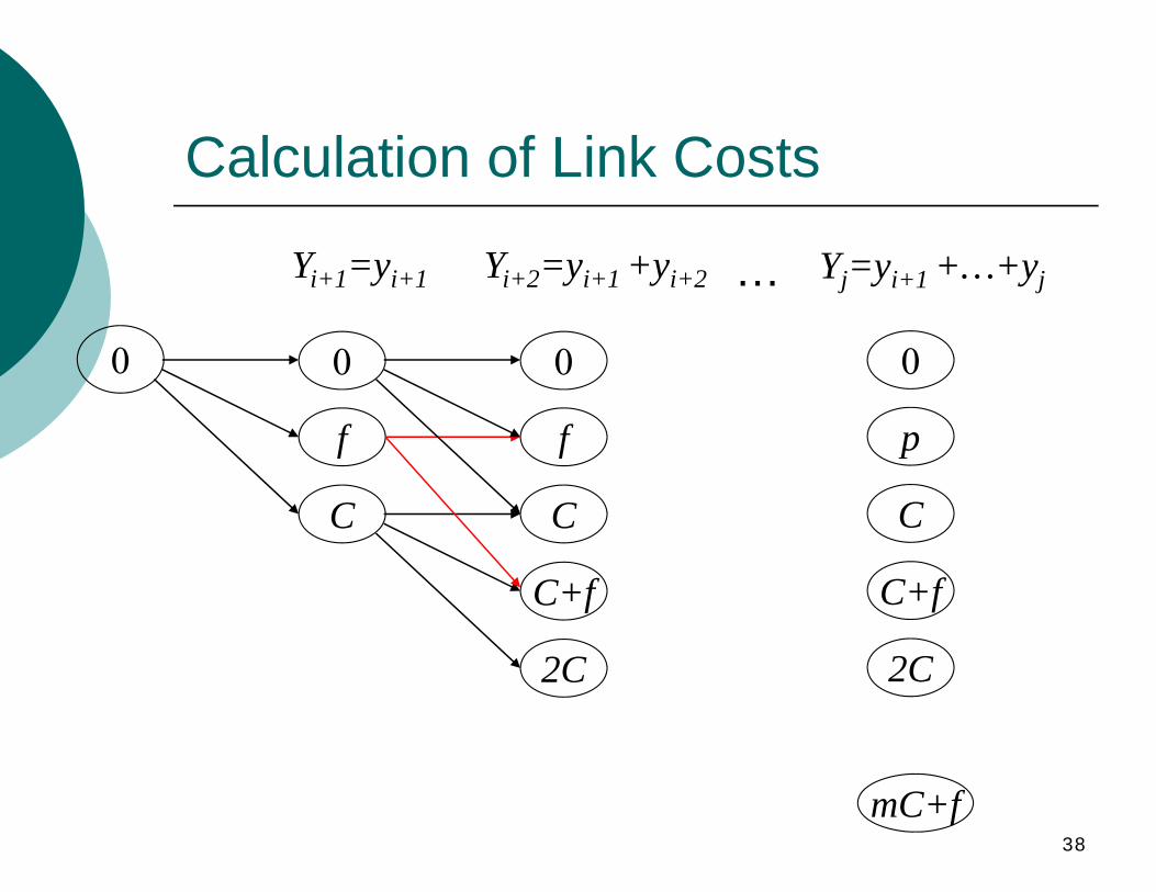
00
f
0
ff
C
f
C
C+f
2C2C
Calculation of Link Costs
Yi+1=yi+1 Yi+2=yi+1 +yi+2 … Yj=yi+1 +…+yj
0
pp
C
C+f
2C2C
mC+f 38

Complexity: equal capacity
{ Computing link cost lij: shortest path algorithm:O((j-i)2).
{ i i h i l d iDetermining the optimal production sequence bbetween all pairs of periods: O(T2)× O(T2) = O(T4).
{ Shortest path algorithm on the whole network : O(T2).
{ CCompllexitit y ffor fifi di nding an opti timall so l ti lution ffor DELS DELS model with equal capacity: O(T4) + O(T2) = O(T4).
{ With a sophisticated algorithm: O(T 3) .
Not applilicablble to problems wi h ith time-ddependdent capaciity{ bl i constraints, why? 39
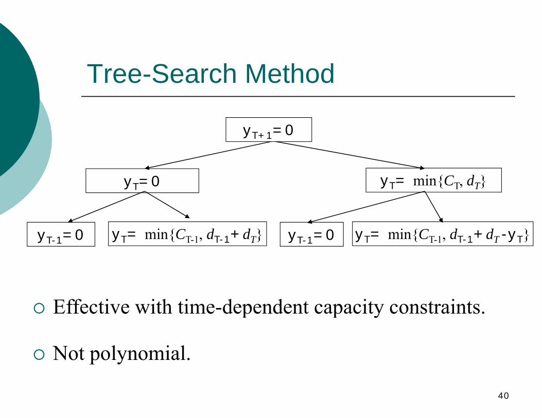
Tree-Search Method
yT+1=0
yT=0 yT = min{CT, dT}
yT-1=0 yT = min{CT-1, dT-1+dT} yT-1=0 yT = min{CT-1, dT-1+dT -yT}
{ Effective with time-dependent capacity constraints{ Effective with time dependent capacity constraints.
{ Not polynomial.p y
40

ZICO Policy
{ Theorem: Any optimal policy is a ZICO policy, I (C y ) y 0 for t 1 TIt-1 · (Ct-yt) · yt = 0, for t=1,…,T.
{ Corollary: If (y1, y2,… yT) represents an optimal solution, and t = max{j: yj>0}, thenj
yt = min{Ct, dt +…+dT}.
41
MIT OpenCourseWarehttp://ocw.mit.edu
ESD.273J / 1.270J Logistics and Supply Chain Management Fall 2009
For information about citing these materials or our Terms of Use, visit: http://ocw.mit.edu/terms.


