Lombardi Drawings of Graphs

Christian A. Duncan1, David Eppstein2, Michael T. Goodrich2,Stephen G. Kobourov3, and Martin Nollenburg2

1Department of Computer Science, Louisiana Tech. Univ., Ruston, Louisiana, USA2Department of Computer Science, University of California, Irvine, California, USA

3Department of Computer Science, University of Arizona, Tucson, Arizona, USA

Abstract. We introduce the notion of Lombardi graph drawings, named after theAmerican abstract artist Mark Lombardi. In these drawings, edges are representedas circular arcs rather than as line segments or polylines, and the vertices haveperfect angular resolution: the edges are equally spaced around each vertex. Wedescribe algorithms for finding Lombardi drawings of regular graphs, graphs ofbounded degeneracy, and certain families of planar graphs.

1 IntroductionThe American artist Mark Lombardi [19] was famous for his drawings of social net-works representing conspiracy theories. Lombardi used curved arcs to represent edges,leading to a strong aesthetic quality and high readability. Inspired by this work, we intro-duce the notion of a Lombardi drawing of a graph, in which edges are drawn as circulararcs with perfect angular resolution: consecutive edges are evenly spaced around eachvertex. While not all vertices have perfect angular resolution in Lombardi’s work, theeven spacing of edges around vertices is clearly one of his aesthetic criteria; see Fig. 1.

Traditional graph drawing methods rarely guarantee perfect angular resolution, butpoor edge distribution can nevertheless lead to unreadable drawings. Additionally, whilesome tools provide options to draw edges as curves, most rely on straight-line edges,and it is known that maintaining good angular resolution can result in exponential draw-ing area for straight-line drawings of planar graphs [12,20]. Our requirement of perfectangular resolution forces us to use curved edges, since even very simple graphs such ascycle graphs cannot be drawn with perfect angular resolution and straight edges.

Fig. 1: Mark Lombard, George W. Bush, Harken Energy, and Jackson Stevens c.1979-90, 1999. Graphite on paper, 20×44 inches [19].

New Results. We define a Lombardi drawing of a graph G to be a drawing of Gin the plane in which vertices are represented as points (or as disks or labels centeredon those points), edges are represented as line segments or circular arcs between theirendpoints, and every vertex has perfect angular resolution, as measured by the angleformed by the tangents to the edges at the vertex. We do not necessarily insist that thedrawings are free of crossings; the drawings of Lombardi had crossings, sometimeseven in cases where they could have been avoided. We also do not consider crossingswhen we measure the angular resolution of a drawing. However, we do require that theonly vertices that intersect the arc for an edge (u,v) are its two endpoints u and v.

Several of Mark Lombardi’s drawings used a circle as their overall shape. We definea circular Lombardi drawing to be a Lombardi drawing in which the vertices lie on acircle. Similarly, we define a k-circular Lombardi drawing to be a Lombardi drawingin which the vertices lie on k concentric circles. We provide the following:

– We characterize the regular graphs that have circular Lombardi drawings, and wefind efficient algorithms for constructing these drawings.

– We describe methods of finding Lombardi drawings for any 2-degenerate graph (agraph that may be reduced to the empty graph by repeated removal of vertices ofdegree at most 2) and many but not all 3-degenerate graphs.

– We investigate the graphs that have planar Lombardi drawings. We show that cer-tain subclasses of the planar graphs always have such drawings, but that there existplanar graphs with no planar Lombardi drawing.

– We implement an algorithm for constructing k-circular Lombardi drawings and useit to draw many symmetric graphs.

Related Work. Although most previous work on angular resolution concerns straight-line drawings (e.g., see [8,12,20]) or polyline drawings (e.g., see [13,16]), the angu-lar resolution of drawings with circular-arc edges was previously studied by Chenget al. [6], who showed that maintaining bounded angular resolution in planar draw-ings may require exponential area even with circular-arc edges. Our circular Lombardidrawings use a circular layout of vertices that is already popular (e.g., see [3,11,25]).However, previous methods for circular layouts draw edges as straight line segments orcurves perpendicular to the circle, neither of which leads to good angular resolution.

Efrat et al. [9] show that given a fixed placement of the vertices of a planar graph,determining whether the edges can be drawn with circular arcs so that there are no cross-ings is NP-Complete. Brandes and Schlieper [5] use force-directed algorithms to max-imize the angular resolution of fixed-position drawings, and Di Battista and Vismaragive an nonlinear optimization characterization that can find straight-line drawings ofembedded planar graphs with a prescribed assignment of angles if such drawings ex-ist. Aicholzer et al. [1] show that, for a given embedded planar triangulation with fixedvertex positions, one can find a circular-arc drawing of the triangulation that maximizesthe minimum angular resolution by solving a linear program.

Any tree may be drawn with straight edges and perfect angular resolution. However,in a separate paper under submission, we show that (when the order of the edges is fixedaround each vertex) straight-line tree drawings with perfect angular resolution may re-quire exponential area, whereas Lombardi drawings can achieve polynomial area.

2

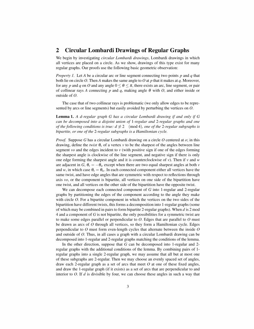
2 Circular Lombardi Drawings of Regular GraphsWe begin by investigating circular Lombardi drawings, Lombardi drawings in whichall vertices are placed on a circle. As we show, drawings of this type exist for manyregular graphs. Our proofs use the following basic geometric observation:

Property 1. Let A be a circular arc or line segment connecting two points p and q thatboth lie on circle O. Then A makes the same angle to O at p that it makes at q. Moreover,for any p and q on O and any angle 0≤ θ ≤ π , there exists an arc, line segment, or pairof collinear rays A connecting p and q, making angle θ with O, and either inside oroutside of O.

The case that of two collinear rays is problematic (we only allow edges to be repre-sented by arcs or line segments) but easily avoided by perturbing the vertices on O.

Lemma 1. A d-regular graph G has a circular Lombardi drawing if and only if Gcan be decomposed into a disjoint union of 1-regular and 2-regular graphs and oneof the following conditions is true: d 6≡ 2 (mod 4), one of the 2-regular subgraphs isbipartite, or one of the 2-regular subgraphs is a Hamiltonian cycle.

Proof. Suppose G has a circular Lombardi drawing on a circle O centered at o; in thisdrawing, define the twist θv of a vertex v to be the sharpest of the angles between linesegment vo and the edges incident to v (with positive sign if one of the edges formingthe sharpest angle is clockwise of the line segment, and negative sign if there is onlyone edge forming the sharpest angle and it is counterclockwise of v). Then if v and ware adjacent in G, θv =−θw except when there are two equal sharpest angles at both vand w, in which case θv = θw. In each connected component either all vertices have thesame twist, and have edge angles that are symmetric with respect to reflections throughaxis vo, or the component is bipartite, all vertices on one side of the bipartition haveone twist, and all vertices on the other side of the bipartition have the opposite twist.

We can decompose each connected component of G into 1-regular and 2-regulargraphs by partitioning the edges of the component according to the angle they makewith circle O. For a bipartite component in which the vertices on the two sides of thebipartition have different twists, this forms a decomposition into 1-regular graphs (someof which may be combined in pairs to form bipartite 2-regular graphs). When d is 2 mod4 and a component of G is not bipartite, the only possibilities for a symmetric twist areto make some edges parallel or perpendicular to O. Edges that are parallel to O mustbe drawn as arcs of O through all vertices, so they form a Hamiltonian cycle. Edgesperpendicular to O must form even-length cycles that alternate between the inside Oand outside of O. Thus, in all cases a graph with a circular Lombardi drawing can bedecomposed into 1-regular and 2-regular graphs matching the conditions of the lemma.

In the other direction, suppose that G can be decomposed into 1-regular and 2-regular graphs with the additional conditions of the lemma. By combining pairs of 1-regular graphs into a single 2-regular graph, we may assume that all but at most oneof these subgraphs are 2-regular. Then we may choose an evenly spaced set of angles,draw each 2-regular graph as a set of arcs that meet O at one of these fixed angles,and draw the 1-regular graph (if it exists) as a set of arcs that are perpendicular to andinterior to O. If d is divisible by four, we can choose these angles in such a way that

3

no angle is parallel to the circle O and no angle is perpendicular to O. If d is odd, theangles can be chosen so that the 1-regular subgraph of G is perpendicular to and interiorto O, and all other angles are neither perpendicular nor parallel to O. If d is congruent to2 mod 4 and one of the 2-regular graphs is a Hamiltonian cycle, we may draw it usingedges that lie on C, placing the vertices in the order of this cycle. And if d is congruentto 2 mod 4 and one of the 2-regular graphs is bipartite, we may draw it using edges thatare perpendicular to O, taking care in the vertex placement to avoid using an edge thatconnects two diametrally opposite points on O via an exterior arc. In both of these caseswhere d is 2 mod 4 we then draw the other subgraphs of the decomposition using arcsthat are neither parallel to nor perpendicular to O. ut

Theorem 1. Every regular graph G of degree divisible by four has a circular Lombardidrawing. A regular graph of odd degree has a circular Lombardi drawing if and onlyif it has a perfect matching. A regular graph of degree congruent to two modulo fourhas a circular Lombardi drawing if and only if it is Hamiltonian or has a 2-regularbipartite subgraph. In the cases of odd degree and degree divisible by four, when acircular Lombardi drawing exists it can be constructed in polynomial time.

Proof. This follows from Lemma 1 together with Petersen’s theorem that a regulargraph of even degree can always be decomposed into 2-regular subgraphs [22,23]. ut

Testing for the existence of a 2-regular bipartite subgraph in a regular graph is NP-complete (in 3-regular graphs, it is equivalent to 3-edge-coloring) but we have not de-termined its complexity for the case of interest to us, d-regular graphs in which d iscongruent to two modulo four.

Figures 2(a–c) show drawings produced by this method for 3-regular, 4-regular,and 6-regular graphs. Figure 2(d) shows a 3-regular graph that does not have a perfectmatching, and that therefore has no circular Lombardi drawing.

(a) (b) (c) (d)

Fig. 2: (a) A circular Lombardi drawing of the 3-regular Wagner graph; (b) A circularLombardi drawing of the 4-regular graph K4,4; (c) The 6-regular Paley graph connectingintegers modulo 13 if their difference is a quadratic residue; (d) A 3-regular graph thathas no perfect matching and therefore has no circular Lombardi drawing.

4

For bipartite regular graphs of bounded degree the method of Theorem 1 again leadsto a linear-time algorithm.

Corollary 1. Every bipartite d-regular graph has a circular Lombardi drawing thatcan be constructed in time O(dn logd).

Proof. It is known that every bipartite regular graph can be decomposed into perfectmatchings in the given time bound [2,7,24].1 The result follows by applying Theorem 1to this decomposition. ut

Corollary 2. Every d-regular graph for which d is a power of two, with the exceptionof 2-regular non-bipartite disconnected graphs, has a circular Lombardi drawing thatcan be constructed in time O(dn logd).

Proof. Repeatedly decompose the graph into pairs of subgraphs with half the degreeby taking alternating edges of an Euler tour [10] and then apply Theorem 1 to thedecomposition. ut

Corollary 3. Every 3-regular bridgeless graph has a circular Lombardi drawing thatcan be constructed in time O(n log3 n log logn).

Proof. The result that every 3-regular bridgeless graph has a perfect matching (equiva-lently, a decomposition into a 2-regular and a 1-regular subgraph) is known as Petersen’stheorem [23]. Such a matching can be found in the stated time bound via an algorithmbased on dynamic 2-edge-connectivity testing data structures [4,15,26]. ut

3 Two-Degenerate and Three-Degenerate GraphsThe degeneracy of a graph G is the minimum number d such that G can be reduced tothe empty graph by repeatedly removing a vertex of degree at most d; equivalently, itis the minimum degree in the subgraph of G that maximizes the minimum degree [18].If a graph G has degeneracy at most d, it is known as d-degenerate. In this section weconsider algorithms for drawing 2-degenerate and 3-degenerate graphs, with a specifiedcyclic ordering of the edges around each vertex. The main idea of these algorithms isto delete a low-degree vertex, draw the remaining graph with the appropriate angles ateach of its vertices, and then find a position for the deleted vertex that allows it to beconnected to the drawing of the remaining graph.

For 2-degenerate graphs, when we add back the vertices in reverse order of deletion,there is always a circle on which they can be added so we can choose one point on thecircle that is not crossed by a previously drawn feature. For 3-degenerate graphs thereare two points at which the point can be added to give the correct edge angles (the com-mon intersection points of three circles) so there might be circumstances under whichthis addition is forced to create an undesirable edge-vertex or vertex-vertex intersection.

The results in this section rely on the following geometric property; we defer theproof to the appendix.

1 The fact that every regular bipartite graph has a decomposition into matchings is commonly at-tributed to Konig [17], but is equivalent to a result proved in terms of point-line configurationsin the 1894 Ph.D. thesis of Ernst Steinitz.

5

Property 2. Suppose we are given two points p and q with associated vectors vp andvq and an angle θpq. Consider all pairs of circular arcs that leave p and q with tangentvectors vp and vq respectively and meet at an angle θpq. The locus of meeting points forthese pairs of arcs is a circle.

3.1 2-Degenerate GraphsTheorem 2. Every 2-degenerate graph with a specified cyclic ordering of the edgesaround each vertex has a Lombardi drawing.

Proof. Order the vertices by repeatedly removing a low-degree vertex. Reinsert thevertices in reverse order creating subgraphs G0,G1 . . .Gn with the invariant that aftereach insertion the drawing is a partial Lombardi drawing Γi of Gi where some verticesmay not yet have all of their neighbors placed. To insert a new vertex v = vi+1 withdegree two in Gi+1 (the case for degree one is simpler) let p and q be its two neighborsin Gi+1. Since there is a specified ordering around p, which has already been placedin Γi, there is a unique tangent vector vp associated with the arc from p to v. Similarly,there is a unique tangent vector vq. In addition, since the degree of v in G is known andthe ordering of the neighbors at v is also given, there is a unique angle θpq associatedwith the two arcs from p and q to v. From Property 2, we may choose to place v at anyposition on the defined circle. Choosing a point v that does not coincide with any otherarcs or vertices already placed guarantees we have a valid drawing Γi+1. ut

Corollary 4. Every outerplanar or series-parallel graph has a Lombardi drawing.

Proof. This follows from the fact that these graphs are 2-degenerate. ut

3.2 3-Degenerate GraphsAn algorithm following the same approach can be used to draw many, but not all, 3-degenerate graphs. In this case we have three points p, q, and r that we want to connectby arcs to an unplaced new vertex v. Each pair of known points yields a circle of possi-ble choices for v. These three circles, Opq,Opr,Oqr, have to pairwise cross, and wherethey cross the third one must also cross because fixing the angles between two pairs ofincoming arcs at the new point fixes all angles. Every graph with maximum degree fouris either 4-regular or 3-degenerate, so the same algorithm applies in this case.

However, for certain graphs and certain orderings of the edges around the verticesof the graph, this algorithm can fail by placing a vertex on another edge or vertex. Anexample in which this occurs is the seven-vertex split graph G7 formed by adding fourindependent vertices p, q, r, and s to a triangle xyz, with an edge from each of p, q, r, ands to each of x, y, and z, as shown in Figure 3. In any Lombardi drawing of G7 with theedge order as shown, we can assume by making an appropriate Mobius transformationof the drawing that xyz is equilateral. It follows that the only possible locations for p,q, r, and s are the centroid of the equilateral triangle and the point at infinity, so at leasttwo vertices would have to be placed at the same point, forming an invalid drawing.

6

(a) (b) (c)

Fig. 3: A 7-vertex 3-degenerate graph that has no Lombardi drawing with the givenvertex ordering. (a) A Mobius transformation makes one triangle equilateral, forcingthe other 4 vertices to be placed at the centroid and the point at infinity; (b) A differenttransformation with finite vertex locations; (c) A straight-line drawing of the graph.

4 Non-Crossing Lombardi Drawings4.1 Planar Graphs Without Planar Lombardi DrawingsNot every planar graph has a planar Lombardi drawing. To see this, consider the k-nested triangle graphs, maximal planar graphs with 3k vertices formed by k nestedtriangles with k−1 6-cycles connecting consecutive triangles. A k-nested triangle graphmay also be formed geometrically by gluing k−1 octahedra end-to-end.

As can be seen in Figure 4, the 2-nested and 3-nested triangle graphs have planarLombardi drawings. The 4-nested triangle graph, however, does not. If it did have such adrawing, its middle two triangles would form circles (the only smooth curve formed bythree circular arcs). By an appropriate Mobius transformation, the outer circle O can beassumed to have its three vertices equally spaced around it. The three cirles C1, C2, andC3 that (by Property 2) describe the potential positions of the vertices on the inner circlehave the same radius as O and meet at the center of O, and the inner circle would haveto be tangent to all three of C1, C2, and C3. However, the only circle tangent to all threeis exterior to O, concentric with O and having twice the radius of O. Therefore, usingan edge ordering around each vertex that comes from a planar embedding but enforcingperfect angular resolution leads to a nonplanar drawing, shown in Figure 4(c).

(a) k = 2 (b) k = 3 (c) k = 4

Fig. 4: k-nested triangle graphs. The 2-nested and 3-nested triangle graphs haveplanar Lombardi drawings, but the 4-nested triangle graph does not.

7

(a) (b)

Fig. 5: (a) A good hyperbolic drawing of a seven-node tree, with the dominance regionsof two leaves of the tree shown as shaded regions; (b) The Lombardi drawing formedby adding arcs outside the Poincare model, at 30◦ angles to the boundary, connectingconsecutive leaves.

4.2 Halin GraphsA Halin graph [14] is a planar graph obtained from a plane tree T (with at least fourvertices and with no vertices of degree 2), by connecting all the leaves of T into acycle in the order given by its embedding. As we now describe, Halin graphs (and thegraphs formed in the same way from trees with degree-2 vertices) have planar Lombardidrawings that can be constructed using hyperbolic geometry.

We draw T within a Poincare disk model of the hyperbolic plane, with its leaveson the boundary circle of the model, and then draw the cycle connecting the leavesoutside this circle. If T is drawn using hyperbolic line segments, with perfect angularresolution, then its edges will form circular arcs in the Poincare model; the conformal(angle-preserving) nature of the Poincare model implies that the angular resolution ofthe hyperbolic line segments equals the angular resolution of these Euclidean arcs.

For a given straight-line drawing of a rooted tree in the hyperbolic plane, and a non-root vertex v, partition the hyperbolic plane into wedges bounded by the bisectors ofthe angles around the parent of v and define the dominance region of v to be the wedgecontaining v. Equivalently, in a Voronoi diagram generated by the rays from the parentof v to its children, the dominance region of v is the Voronoi cell containing v. We definea good hyperbolic drawing of a rooted tree T to be a drawing in which the edges arestraight line segments or rays in the hyperbolic plane, the leaves are placed on the circleat infinity, and the dominance regions for two vertices v and w are either nested withineach other (if one of the two vertices is an ancestor of the other) or disjoint otherwise.Two dominance regions in a good hyperbolic drawing are shown in Figure 5(a).

Lemma 2. Every rooted tree has a good hyperbolic drawing.

Proof. We use induction on the number of non-leaf nodes in the given tree T . As a basecase, when there is one non-leaf node, it may be placed at the center of the Poincaredisk model of the hyperbolic plane with its leaves at the limit points of equally-spacedrays (radii of the disk model). Otherwise, let v be a non-leaf that is as far from theroot of T as possible, and let T ′ be formed from T by removing all children of v. Then

8

by induction, T ′ has a good hyperbolic drawing. In this drawing, v is on the circle atinfinity; let R be the ray connecting the parent of v to v. For any position x along thisray, let θx be the maximum angle made to R by a line that stays within the dominanceregion of v. Then θx varies continuously along R, starting from a value of π/d at theparent of v (where d is the degree of the parent) and ending with a value of π at v itself.If the degree of v in T is d′, there must be an intermediate position x on R for whichθx = π(1− 1/d′). If we move v to x and place its leaf children at the limit points ofequally spaced rays around x, the result is a good hyperbolic drawing of T . ut

Theorem 3. Every Halin graph has a planar Lombardi drawing that may be con-structed in linear time.

Proof. Root the tree T at an arbitrarily chosen non-leaf node, and construct a goodhyperbolic drawing of T according to Lemma 2. Draw the cycle connecting the leavesof T using circular arcs that meet the circle bounding the Poincare model at anglesof 30◦ as in Figure 5(b). Then each non-leaf node of T has perfect angular resolutionfrom the tree drawing, and each leaf node has perfect angular resolution because the rayconnecting it to its parent in T is perpendicular to the boundary circle and therefore at120◦ angles from the two arcs connecting it to adjacent leaves. ut

4.3 Other Classes of Planar GraphsThe networks formed by two-dimensional soap bubbles naturally form 3-regular planarLombardi drawings: they have circular arcs as their edges (the boundaries betweenbubbles), and 120◦ angles at each vertex where three arcs meet [21]. However, we donot have a precise characterization of the graphs that can be formed in this way.

The vertices of every Platonic solid, Archimedean solid, and prism lie on a commonsphere. In all but two cases (the snub cube and snub dodecahedron) one may draw theedges of the polyhedron as circular arcs on the sphere with perfect angular resolution.By stereographic projection, each of these graphs has a Lombardi drawing in the plane.For instance, Figure 4(a) depicts the graph of the octahedron drawn in this way.

All outerplanar and series-parallel graphs have Lombardi drawings (Corollary 4),but we do not know whether they all have planar Lombardi drawings.

5 The Lombardi SpirographWe have implemented a program for constructing k-circular Lombardi drawings ofgraphs with dihedral symmetry; we call it the Lombardi Spirograph, as its drawingsresemble those created by the SpirographTM drawing toy produced by Hasbro, Inc. Ourprogram places vertices on k concentric circles; the input specifies not only the num-ber of vertices per circle and the set of edges to be drawn, but also the order in whichthose edges are incident at each vertex. Each vertex can have at most three neighbors onsmaller circles; a circle on which the vertices have two or three inward neighbors has aunique radius for which the vertices have perfect angular resolution, whereas the radiusfor circles on which the vertices have one inner neighbor is chosen heuristically.

Figures 2 (a–c), 4 (a & b), and 6 were all drawn using this program.

9

(a) Petersen graph (b) K6 (c) Grotzsch graph

(d) Nauru graph G(12,5) (e) Brinkmann graph

(f) Dyck graph (g) 40-vertex cubic symmetric graph F40 (thebipartite double cover of the dodecahedron)

Fig. 6: Sample drawings by the Lombardi Spirograph.

10

6 ConclusionsWe have begun an investigation into Lombardi drawings and found algorithms basedon graph matching, incremental construction, hyperbolic geometry, and symmetry dis-play for constructing drawings of this type. Based on our constructions, we can showthat many regular graphs, sparse graphs, special classes of planar graphs, and sym-metric graphs have Lombardi drawings, and we have found drawings of this type formany well-known graphs. In addition, we have implemented a method for producingLombardi drawings of graphs with dihedral symmetry, which we call the LombardiSpirograph.

There are many related problems that remain open, including the following:

1. What are the complexities of finding circular Lombardi drawings for degrees thatare 2 mod 4?

2. Is there an effective classification of 3-degenerate graphs according to whether theycan or cannot be drawn in a way that avoids overlapping features?

3. Are there efficient methods for producing planar Lombardi drawings for outerpla-nar graphs, series-parallel graphs, and 3-regular planar graphs?

It would also be of interest to combine Lombardi drawing with other standard graphdrawing quality criteria such as edge-length minimization. In general, we believe thatLombardi drawings will be a fruitful area for much additional research.

AcknowledgmentsThis research was supported in part by the National Science Foundation under grant0830403, by the Office of Naval Research under MURI grant N00014-08-1-1015, andby the German Research Foundation under grant NO 899/1-1.

References1. O. Aichholzer, W. Aigner, F. Aurenhammer, K. C. Dobiasova, and B. Juttler. Arc

triangulations. Proc. 26th Eur. Worksh. Comp. Geometry (EuroCG’10), pp. 17–20, 2010.2. N. Alon. A simple algorithm for edge-coloring bipartite multigraphs. Information

Processing Letters 85(6):301–302, 2003, doi:10.1016/S0020-0190(02)00446-5.3. M. Baur and U. Brandes. Crossing reduction in circular layouts. Proc. 30th Int. Worksh.

Graph-Theoretic Concepts in Computer Science (WG 2004), pp. 332–343. Springer-Verlag,LNCS 3353, 2005, http://www.springerlink.com/content/fepu2a3hd195ffjg/.

4. T. C. Biedl, P. Bose, E. D. Demaine, and A. Lubiw. Efficient algorithms for Petersen’smatching theorem. J. Algorithms 38(1):110–134, 2001, doi:10.1006/jagm.2000.1132.

5. U. Brandes and B. Schlieper. Angle and distance constraints on tree drawings. Proc. 14thSymposium on Graph Drawing (GD 2006), pp. 54–65. Springer-Verlag, LNCS 4372, 2007,doi:10.1007/978-3-540-70904-6 7.

6. C. C. Cheng, C. A. Duncan, M. T. Goodrich, and S. G. Kobourov. Drawing planar graphswith circular arcs. Discrete Comput. Geom. 25(3):405–418, 2001,doi:10.1007/s004540010080.

7. R. Cole, K. Ost, and S. Schirra. Edge-coloring bipartite multigraphs in O(ElogD) time.Combinatorica 21(1):5–12, 2001, doi:10.1007/s004930170002.

11

8. G. Di Battista and L. Vismara. Angles of planar triangular graphs. SIAM J. Discrete Math.9(3):349–359, 1996, doi:10.1137/S0895480194264010.

9. A. Efrat, C. Erten, and S. G. Kobourov. Fixed-location circular arc drawing of planargraphs. J. Graph Algorithms Appl. 11(1):145–164, 2007,http://jgaa.info/accepted/2007/EfratErtenKobourov2007.11.1.pdf.

10. H. N. Gabow. Using Euler partitions to edge color bipartite multigraphs. Int. J. ParallelProgramming 5(4):345–355, 1976, doi:10.1007/BF00998632.

11. E. R. Gansner and Y. Koren. Improved circular layouts. Proc. 14th Int. Symp. GraphDrawing (GD 2006), pp. 386–398. Springer-Verlag, LNCS 4372, 2007,doi:10.1007/978-3-540-70904-6 37.

12. A. Garg and R. Tamassia. Planar drawings and angular resolution: algorithms and bounds.Proc. 2nd Eur. Symp. Algorithms, pp. 12–23. Springer-Verlag, LNCS 855, 1994,doi:10.1007/BFb0049393.

13. C. Gutwenger and P. Mutzel. Planar polyline drawings with good angular resolution. Proc.6th Int. Symp. on Graph Drawing (GD’98), pp. 167–182. Springer-Verlag, LNCS 1547,1998, doi:10.1007/3-540-37623-2 13.

14. R. Halin. Uber simpliziale Zerfallungen beliebiger (endlicher oder unendlicher) Graphen.Math. Ann. 156(3):216–225, 1964, doi:10.1007/BF01363288.

15. J. Holm, K. de Lichtenberg, and M. Thorup. Poly-logarithmic deterministic fully-dynamicalgorithms for connectivity, minimum spanning tree, 2-edge, and biconnectivity. J. ACM48(4):723–760, 2001, doi:10.1145/502090.502095.

16. G. Kant. Drawing planar graphs using the canonical ordering. Algorithmica 16:4–32, 1996,doi:10.1007/BF02086606.

17. D. Konig. Grafok es matrixok. Matematikai es Fizikai Lapok 38:116–119, 1931.18. D. R. Lick and A. T. White. K-degenerate graphs. Canad. J. Math. 22:1082–1096, 1970,

http://www.smc.math.ca/cjm/v22/p1082.19. M. Lombardi and R. Hobbs. Mark Lombardi: Global Networks. Independent Curators,

2003.20. S. Malitz and A. Papakostas. On the angular resolution of planar graphs. SIAM J. Discrete

Math. 7(2):172–183, 1994, doi:10.1137/S0895480193242931.21. F. Morgan. Soap bubbles in R2 and in surfaces. Pacific J. Math. 165(2):347–361, 1994,

http://projecteuclid.org/euclid.pjm/1102621620.22. H. M. Mulder. Julius Petersen’s theory of regular graphs. Discrete Mathematics

100(1-3):157–175, 1992, doi:10.1016/0012-365X(92)90639-W.23. J. Petersen. Die Theorie der regularen Graphs. Acta Math. 15(1):193–220, 1891,

doi:10.1007/BF02392606.24. A. Schrijver. Bipartite edge coloring in O(∆m) time. SIAM J. Comput. 28(3):841–846,

1999, doi:10.1137/S0097539796299266.25. J. M. Six and I. G. Tollis. A framework for circular drawings of networks. Proc. 7th

Symposium on Graph Drawing (GD 1999), pp. 107–116. Springer-Verlag, LNCS 1731,1999, doi:10.1007/3-540-46648-7 11.

26. M. Thorup. Near-optimal fully-dynamic graph connectivity. Proc. 32nd ACM Symp.Theory of Computing (STOC ’00), pp. 343–350, 2000, doi:10.1145/335305.335345.

12

A Additional Proofs and FiguresWe now present the proof for Property 2.

Proof (Of Property 2). Let r1 be the meeting point of one such pair of arcs. Let O bethe circle defined by the three points p, q, and r1. From Property 1, the angle θp that thearc from p makes with O as it leaves p is the same as when it arrives at r1. Similarly,let θq be the angle of the arc with O at both q and r1. Therefore, we know that the angleformed by the intersection of the two arcs at r1 is θpq = π−θp−θq; see Fig. 7(a).

p

qr1

θpθq

θpqθp

θq

(a)

vpθp

x

vq

θq

x

x x

θpq

r

qp

(b)

Fig. 7: (a) Angle calculation; (b) Circle construction.

Now, for any other point r2 on O, a circular arc from p through r2 with the sameoutgoing tangent vector vp must again form the same angle θp with O at both p andr2. The same holds for the angle θq at q and r2. Therefore, the angle formed by theintersection of the two arcs at r2 is also θpq.

We can also determine the equation for this circle O. Our goal is to calculate theangle formed by the center of O and the two points p and q. From that, we can use basictrigonometry to calculate the position of the center based on the positions of p and q.For simplicity, assume that the two fixed points p and q are horizontally aligned; seeFig. 7(b). Let r be the point on O halfway between p and q. Since r lies directly abovethe center of the circle, we know that the desired angle is exactly 2x, where x is the angleformed by the horizontal line (from p to q) and the tangent to O at p (or q). From vp,we know the angle, say θph, between the outgoing arc from p and the horizontal line.In Fig. 7(b), this corresponds to the angle θp +x. Similarly we have angle θqh = θq +x.

Finally, from above, we know the angle at r is θpq = π − θp − θq. Solving for x,yields that 2x = θph +θqh−θp−θq = θph +θqh +θpq−π . ut

13