Page 1
LONDON INTERBANK OFFERED RATE Financial Markets & Instruments
2012
Jaime Arimany (FIN3560-01), Maxwell Rispoli (FIN3560-02)
Joshua Street (FIN3560-02), Matthew Vacaro (FIN3560-01)
Babson College
12/3/2012
Page 2
1
Executive Summary
The London Interbank Offered Rate (Libor) is considered the worldwide benchmark for
interest rates. Not only does this key bank interest rate impact major US indices, derivative
markets, and adjustable rate mortgages, but it also accounts for trillions of dollars in loans under
its influence. The Libor was officially recognized as a benchmark rate in 1989 because of the
increased activity in swap derivative and overnight trading. The Libor rate was becoming
progressively more popular with trading centers around the world that involved many different
currencies and markets. This ultimately inspired global markets to follow it as a guideline for
interest setting worldwide due to its collaborative and joint nature with banks in different
countries. Unfortunately, the Libor is considered fundamentally flawed by many- including
current US Federal Reserve Chairman Ben Bernanke- due to its manipulative nature and lack of
regulation1.
In running statistical analysis, we initially believed that the 6-month Treasury bill and the
6-month Libor would be highly correlated between 1990 to present day. Analysis showed that
both rates were highly correlated as a whole (R2 of 96.84%) throughout the years of 1989-2012.
In separating the data for the Libor rate into five year periods, correlation was not as strong
between the years 1995-1999 (R2 of 68.39%). This was most likely attributed to uncertainty in
the interest rate market and the introduction of the euro. For years 2005-2009, there was high
fluctuation in the correlation due to the Libor scandal in the midst of the financial crisis. The
initial hypothesis was correct in relation to the overall correlation, but the results for recent years
have not been as correlated as what they were before the financial crisis and Libor scandal.
1 Staff, and Agencies. "Ben Bernanke and Mervyn King Describe Libor Fixing as 'fraud'" The Guardian. Guardian
News and Media, 17 July 2012.
Page 3
2
Table of Contents
Executive Summary ........................................................................................................................ 1
History of Libor .............................................................................................................................. 3
The Scandal Begins......................................................................................................................... 6
The Aftermath ................................................................................................................................. 7
Statistical Analysis .......................................................................................................................... 9
Six Month Rates ........................................................................................................................ 10
Significant Observations ............................................................................................................... 10
1989-2012.................................................................................................................................. 10
1989-2008.................................................................................................................................. 11
1990-1994.................................................................................................................................. 11
1995-1999.................................................................................................................................. 12
2000-2004.................................................................................................................................. 14
2005-2009.................................................................................................................................. 14
Conclusion .................................................................................................................................... 16
References ..................................................................................................................................... 18
Appendix ....................................................................................................................................... 21
“I pledge my honor that I have neither received nor provided any unauthorized assistance
during the completion of this work.”
“The authors of this paper hereby give permission to Professor Michael Goldstein to distribute
this paper by hard copy, to put it on reserve at Horn Library at Babson College, or to post a
PDF version of this paper on the internet”.
Page 4
3
History of Libor
Known by many as “the Greek banker” who carried out syndicate financing from a new
merchant bank in London during the 1970s, Minos Zombanakis was a financial visionary whose
legacy will long outlive him.2 In 1969, Zombanakis established a branch of Manufacturers
Hannover in London, one of the first banks to operate in the Eurodollar syndicated loan market
that was beginning to gain momentum. He is credited with being one of the first to write a
Eurodollar syndicated loan because of his early deals, specifically the $80 million loan to the
Shaw of Iran.3 The loan to Iran’s central bank was followed by another loan to Italy for $200
million, whose terms became the standard for the industry. The loan to Italy was structured for
five years, with interest rates recalculating semi-annually at a 0.75% premium over a floating
rate that represents market conditions; this floating rate is what Zombanakis called the London
interbank offered rate. 4
The birth of the London interbank offered rate5 came as a necessary product of
combining two types of loans: Eurodollar loans and syndicated loans. The Eurodollar market
emerged in the 1960s as a way for corporate and sovereign borrowers to raise funds while
avoiding taxation and regulation. However, there was a demand for large loans in the Eurodollar
market, some much larger than any one bank would be willing to hold as a portion of their
portfolio. 6
In order to make a loan of this magnitude, a group of lenders had to form a syndicate
2 Eade, Philip. "Minos Zombanakis." Euromoney.358 (1999).
3 Zombanakis is often credited with being the inventor of Eurodollar syndicated loans because of how much he used
and advocated these instruments, even though they were used more than a year earlier by other bankers in Austria. 4 Ridley, Kirstin, and Huw Jones. "A Greek Banker Spills On The Early Days Of The LIBOR And His First Deal
With The Shah Of Iran." www.businessinsider.com. Business Insider, 8 Aug. 2012. 5 The London interbank offered rate can be referred to by a variety of names and abbreviations including Libor,
LIBOR, BBA Libor, BBALIBOR, and bbalibor. This paper will refer to it as Libor. 6 Taaffe, Ouida. "The Life and Good times of LIBOR." - Minos Zombanakis. IFS School of Finance, n.d.
Page 5
4
in which they all contribute funds to one sole borrower.7 Merging the Eurodollar loans and
syndicated loans created new issues that had not been necessary to consider before. To adjust for
changes in market conditions for these loans to be paid off over longer periods to multiple banks,
the interest rate on each loan had to be a floating rate with a premium over a generally accepted
rate that represents the cost of lending.8
Fourteen years after Zombanakis created Libor, global banking trends in 1984 were
characterized by increased trading of new products, such as interest rate swaps, foreign currency
options, and forward rate agreements. Further growth in this London interbank market would
have been inhibited without an element of standardization for these trades; the BBAIRS9 was
established in October of 1984, as a result. 10
Part of the BBAIRS included BBA Interest
Settlement rates, which were the immediate predecessor of the London Interbank Offered Rate.11
Libor has viewed as an industry standard since it was first calculated in 1986.
Libor rate data is available from various private data vendors, even though Thompson
Reuters calculates the rates. To calculate all the rates on London business days for ten different
currencies12
and fifteen borrowing periods13
, contributing banks send their interbank borrowing
rates to Thompson Reuters every day at 11:00AM. In the time before Thompson Reuters
distributes the data at noon, it receives all the data for each borrowing period from different
contributing banks, sorts the data from smallest to largest, removes the upper and lower quartile
7 "Syndicated Loan." Investopedia.com. Investopedia, n.d.
8 Eade, Philip. "Minos Zombanakis." Euromoney.358 (1999).
9 BBAIRS stands for the British Bankers Association Interest Rate Swaps, which acted as the predecessor of
LIBOR. 10
"BBA LIBOR - Frequently Asked Questions (FAQs)." BBA LIBOR. British Bankers Association. 11
"Interest Rate Swaps - Interest Rate, LIBOR Rates, Base Rates, Euribor Rates, Gilt Rates, Historic Rates and
Trends." Www.Swap-Rates.com. CLP Structured Finance, n.d. 12
The ten currencies that LIBOR rates are calculated for include: Pound Sterling (GBP), US Dollar (USD), Japanese
Yen (JPY), Swiss Frank (CHF), Canadian Dollar (CAD), Australian Dollar (AUD), Euro (EUR), Danish Kroner
(DKK), Swedish Krona (SEK), and New Zealand Dollar (NZD). 13
The fifteen borrowing periods range from overnight to one year.
Page 6
5
in an attempt to remove outliers, and finally calculates the mean on the remaining data. This
process, referred to as calculating a ‘shaved’ or ‘trimmed’ mean, is performed 150 times each
day (for the fifteen periods in each of the ten currencies). 14
After calculating, Thompson Reuters
distributes the Libor rates and the rates submitted by the contributing banks to data vendors who
make the information available worldwide.
The current Libor is quite different from when Zombanakis first calculated it over forty
years ago. Aside from the computational differences that come along with currently using a
trimmed mean for rates, Libor today is also notably different based on who uses the rates and for
what purpose. Libor rates are widely used as a benchmark for short-term interest rates and the
settlement of interest rate contracts.15
In addition to the syndicated loans that it was originally
designed for, Libor is used to gauge the cost of unsecured borrowing, as a basis for derivatives
trading, and as a basis for many different types of lending, such as commercial loans and
residential mortgages.16
When Libor was first created, contributing banks had little reason to manipulate the rates
that they were reporting; the potentially destroyed relationship within a syndicate was enough to
prevent the borrower from artificially adjusting the reported rates.17
Until recent years, few have
thought critically about how the Libor rates are being calculated and, more importantly, the
potential of contributing banks to manipulate the reported rates.
14
"BBA LIBOR - Frequently Asked Questions (FAQs)." BBA LIBOR. British Bankers Association, n.d. 15
"Interest Rate Swaps - Interest Rate, LIBOR Rates, Base Rates, Euribor Rates, Gilt Rates, Historic Rates and
Trends." Www.Swap-Rates.com. CLP Structured Finance, n.d. 16
"BBA LIBOR - Frequently Asked Questions (FAQs)." BBA LIBOR. British Bankers Association, n.d. 17
Ridley, Kirstin, and Huw Jones. "A Greek Banker Spills On The Early Days Of The LIBOR And His First Deal
With The Shah Of Iran." Business Insider, 8 Aug. 2012.
Page 7
6
The Scandal Begins
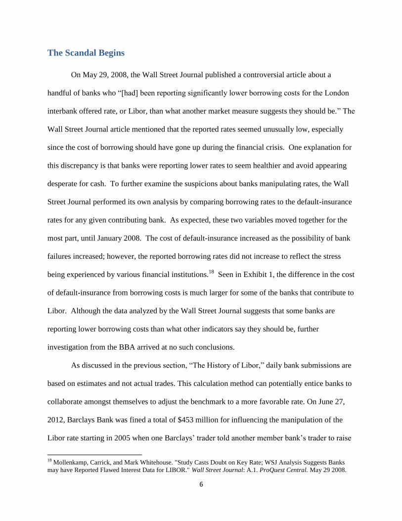
On May 29, 2008, the Wall Street Journal published a controversial article about a
handful of banks who “[had] been reporting significantly lower borrowing costs for the London
interbank offered rate, or Libor, than what another market measure suggests they should be.” The
Wall Street Journal article mentioned that the reported rates seemed unusually low, especially
since the cost of borrowing should have gone up during the financial crisis. One explanation for
this discrepancy is that banks were reporting lower rates to seem healthier and avoid appearing
desperate for cash. To further examine the suspicions about banks manipulating rates, the Wall
Street Journal performed its own analysis by comparing borrowing rates to the default-insurance
rates for any given contributing bank. As expected, these two variables moved together for the
most part, until January 2008. The cost of default-insurance increased as the possibility of bank
failures increased; however, the reported borrowing rates did not increase to reflect the stress
being experienced by various financial institutions.18
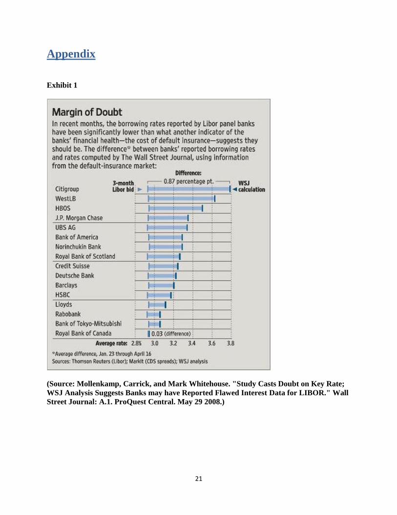
Seen in Exhibit 1, the difference in the cost
of default-insurance from borrowing costs is much larger for some of the banks that contribute to
Libor. Although the data analyzed by the Wall Street Journal suggests that some banks are
reporting lower borrowing costs than what other indicators say they should be, further
investigation from the BBA arrived at no such conclusions.
As discussed in the previous section, “The History of Libor,” daily bank submissions are
based on estimates and not actual trades. This calculation method can potentially entice banks to
collaborate amongst themselves to adjust the benchmark to a more favorable rate. On June 27,
2012, Barclays Bank was fined a total of $453 million for influencing the manipulation of the
Libor rate starting in 2005 when one Barclays’ trader told another member bank’s trader to raise
18
Mollenkamp, Carrick, and Mark Whitehouse. "Study Casts Doubt on Key Rate; WSJ Analysis Suggests Banks
may have Reported Flawed Interest Data for LIBOR." Wall Street Journal: A.1. ProQuest Central. May 29 2008.
Page 8
7
the three-month dollar Libor rate19
. According to a report by the Financial Service Authority
(FSA), a total of 257 requests were made by Barclay’s derivative traders to manipulate Libor and
Euribor rates20
. Further discussion on the specifics of legal actions taken against Barclay’s, and
on the scandal’s aftermath, can be found later in the next section.
In the eve of the financial crisis, Banks became increasingly speculative of other banks’
credit worthiness following the downfall of Northern Rock in September of 2007. In order to
alleviate inter-bank lending tension fueled by a spike in Libor rates, Barclay’s officials requested
member banks to submit low Libor estimates21
. The mentality behind these fraudulent decisions
revolve around the concept that a low Libor rate suggests that banks are confident on the ability
of others to pay back loans. The problem during this time was that increasingly high Libor rates
were attracting scrutiny from the media on the potential weakness of the financial system.
The Aftermath
It is easy to underestimate the colossal influence that the Libor rate has around the world.
To give some perspective on the matter, the total value of securities and loans affected by Libor
sum up to $800 trillion22
while the world’s gross domestic product circles around the $70
trillion23
mark. Libor has an effect on everything from financial institutions’ earnings to the
small loans and payments individual citizens make.
Andrew Lo, professor of finance at the Massachusetts Institute of Technology, said that
the Libor scandal “dwarfs by orders of magnitude any financial scams in the history of
19
The Barclays’ trader said “What’s up with ur guys 34.5 3m fix… tell him to get it up!” 20
"Timeline: Libor-fixing Scandal." BBC News. BBC, 26 Sept. 2012. 21
In December of 2007, a Barclay’s employee reached out to the New York Federal Reserve Bank to express his
concern that his bank was involved in Libor rate-fixing. 22
Fernandez, Tommy. "Libor Pains: What's the Impact?" Money Management Executive 20.32 (2012):
1,n/a. ProQuest Central.Web. 2 Dec. 2012. 23
"Focus: World GDP." The Economist. The Economist Newspaper, n.d. Web. 25 Nov. 2012.
Page 9
8
markets”24
. These manipulations had a universal influence and directly affected pensions, mutual
funds, derivative markets, currencies, adjustable rate mortgages and other financial institutions,
government agencies, and individuals who are influenced by fluctuations of the cost of debt.
Due to the massive discrepancies caused by the Libor scandal, the CFTC “[required]
Barclays to pay a $200 million civil monetary penalty, cease and desist from further violations as
charged, and take specified steps, such as making the determinations of benchmark submissions
transaction-focused (as set forth in the Order), to ensure the integrity and reliability of its Libor
and Euribor submissions and improve related internal controls”25
. These manipulations caused a
complex web of legal actions that are still far from being settled. Vast arrays of companies and
government agencies, such as the California Public Employees’ Retirement System (CalPERS),
have started investigating whether or not they lost money from causes related to Libor rate
manipulation. Other entities, such as the New York Nassau Country have already come forward
saying that a total of $13 million in losses were attributed to these manipulations26
.
The scandal has critically damaged both investor and public confidence in the financial
system. On September 11, 2012, The Times of London reported that “central banks around the
world are establishing a group to monitor the reform of Libor”27
in the scandals aftermath,
although no further details on the specifics have been revealed. In order to restore confidence in
the system, new regulations have to be set in place that specifically addresses the system’s
24
Farrel, Maureen. "Explaining the Libor Interest Rate Mess." CNNMoney. Cable News Network, 03 July 2012 25
"RELEASE: Pr6289-12." CFTC Orders Barclays to Pay $200 Million Penalty for Attempted Manipulation of and
False Reporting concerning Libor and Euribor Benchmark Interest Rates. U.S. Commodity Futures Trading
Commission, 27 June 2012. 26
Grovum, Jake. "More States Dig into Libor Scandal." McClatchy - Tribune News ServiceProQuest Central. Nov
29 2012. Web. 2 Dec. 2012 . 27
Roberts, William. "Report: Central Bankers Form Committee to Monitor Interbank Reform." SNL European
Financials Daily(2012)ProQuest Central. Web. 2 Dec. 2012.
Page 10
9
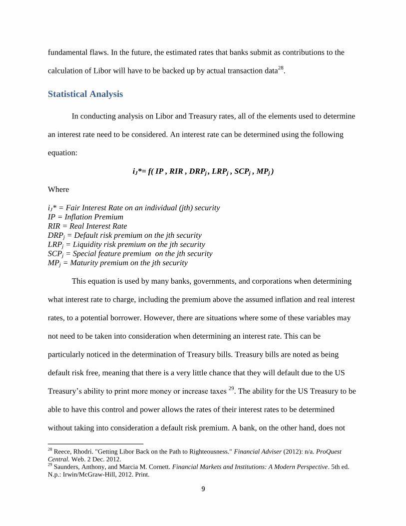
fundamental flaws. In the future, the estimated rates that banks submit as contributions to the
calculation of Libor will have to be backed up by actual transaction data28
.
Statistical Analysis
In conducting analysis on Libor and Treasury rates, all of the elements used to determine
an interest rate need to be considered. An interest rate can be determined using the following
equation:
iJ*= f( IP , RIR , DRPj , LRPj , SCPj , MPj )
Where
iJ* = Fair Interest Rate on an individual (jth) security
IP = Inflation Premium
RIR = Real Interest Rate
DRPj = Default risk premium on the jth security
LRPj = Liquidity risk premium on the jth security
SCPj = Special feature premium on the jth security
MPj = Maturity premium on the jth security
This equation is used by many banks, governments, and corporations when determining
what interest rate to charge, including the premium above the assumed inflation and real interest
rates, to a potential borrower. However, there are situations where some of these variables may
not need to be taken into consideration when determining an interest rate. This can be
particularly noticed in the determination of Treasury bills. Treasury bills are noted as being
default risk free, meaning that there is a very little chance that they will default due to the US
Treasury’s ability to print more money or increase taxes 29
. The ability for the US Treasury to be
able to have this control and power allows the rates of their interest rates to be determined
without taking into consideration a default risk premium. A bank, on the other hand, does not
28
Reece, Rhodri. "Getting Libor Back on the Path to Righteousness." Financial Adviser (2012): n/a. ProQuest
Central. Web. 2 Dec. 2012. 29
Saunders, Anthony, and Marcia M. Cornett. Financial Markets and Institutions: A Modern Perspective. 5th ed.
N.p.: Irwin/McGraw-Hill, 2012. Print.
Page 11
10
have the ability to print money or tax its customers, which gives banks a reason to charge a
default risk premium based on an idea that there is a possibility that they will not be able to be
completely compensated for their investments. The Treasury bill rate seemed like a good
benchmark towards the Libor because it was the minimum rate that people would get back for
investing their money.
Six Month Rates
For this analysis, the use of the 6 month Treasury and 6 month Libor rate will be used.
These two rates have been selected for several reasons. One of the most significant is that there
was no data on the 1 month Treasury bill rate during the 1990s.30
The shortest duration and
maturity in the US Treasury market was instead a 3 month rate. Since this was the shortest, it
was also the most susceptible to short term volatility. Therefore, when selecting data for all of
the points, it was imperative that the credit risk premium was not the highest, lending to the
rationale that the 6 month rate was the best. Given the data from both the Treasury and the BBA,
the 6 month rate was the most readily available and reasonable to use considering the risks to
interest rates discussed previously.
Significant Observations
1989-2012
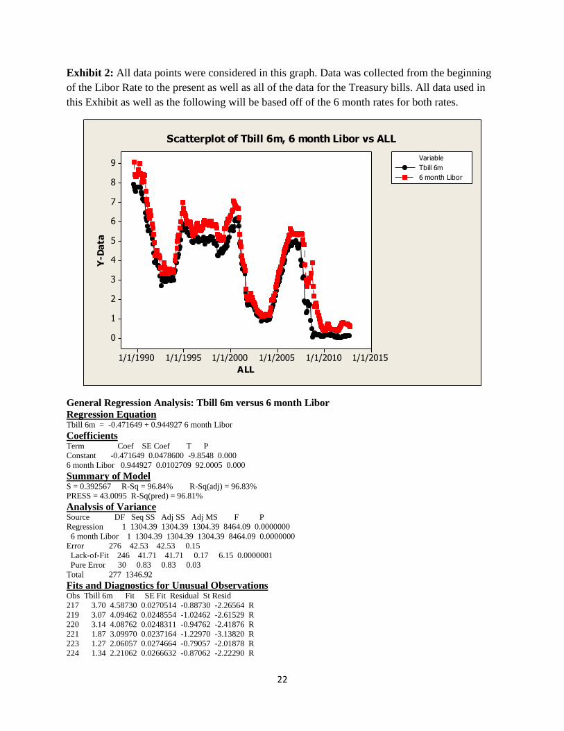
Since the inception of the Libor rate, the correlation to the US Treasury bill has been very
highly correlated. While viewing the data as a whole, over the last twenty-two years the two rates
have remained highly correlated as was observed in the regression model created in Exhibit 2 .
Over the entire life time of the Libor rate, the regression model calculated that the R2 value was
30
http://www.Treasury.gov/resource-center/data-chart-center/interest-
rates/Pages/TextView.aspx?data=yieldYear&year=2001
Page 12
11
extremely high with a value of 96.84% (Exhibit 2). As a generally accepted principle, R2 values
above 0.9 represent a very strong correlation31
. This correlation is also based off of 275 data
points for each rate, giving the analysis a statistically significant amount of points to consider.
However, it is not perfect and when examining the output, fifteen points in close proximity to
each other have been noted by the program as being outliers. These outliers are stated as
‘unusual observations,’ which means that they have standard deviations above 2.0 (Exhibit 2).
These outliers begin to occur in late 2007, perhaps right at the peak of the market bubble before
the collapse of the financial markets in the following year (Exhibit 2). The ‘unusual
observations’ continue all the way through the crisis to 2009, which could indicate that there was
something outside of the normal trend that impacted one of the two rates. The cause of this is
very likely to be that of the Libor Scandal.
1989-2008
Additionally, it can be observed that the correlation rises after removing the data points
where the unusual observations begin. The increase is only incremental, but the rise by 173 basis
points (bps) indicates that this new range, which removed the most recent four years, in fact did
alter the outcome of the regression model (Exhibit 3). By removing data from the tail of this
collection range, the steep drop off is not shown32
which occurred when the financial markets
collapsed.
1990-1994
In this section, the correlation between these two rates for the years of 1990 to 1994 was
very high. According to the analysis, which is noted in Exhibit 4, there was R² of 98.69%, and a
31
"Biz/ed - Correlation Explained [TimeWeb] | Biz/ed." Biz/ed - Correlation Explained [TimeWeb] | Biz/ed. N.p., 2
Nov. 2002. 32
Data sans 07 on
Page 13
12
P-value of 0.000 for this regression model. These strong results show that there is a very large
correlation between these two rates for these years. This is imperative to note because the
Treasury bill, being default risk free, and the Libor, being an arithmetic mean of the interest rates
that banks would pay to borrow money, show that the interest rates are determined in relation to
each other and the high correlation would show that the countries involved in the Libor were not
seeing too much additional risk in their investments during the majority of these years. The mean
of the spread was comparatively low at 0.7011%, which shows that the average difference
between the Libor and Treasury Bill 6 month rates were about 70bps, within a standard deviation
of about 26bps (Exhibit 5).
1995-1999
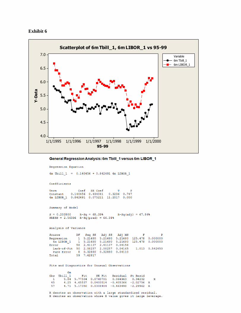
In comparing these two rates for the years of 1995 to 1999, we noticed that there was a
notable weaker correlation. As seen in Exhibit 6, there was an R² of 68.39%, which statistically
speaking is only moderately correlated. The regression model for these years yielded outcomes
where the spread was further apart than in the previous years, as noted in Exhibit 7 where the
spread had a mean of 0.7669 and standard deviation of 0.2097; however, the P-value remained
strong at 0.000. It is also important to note that even though the regression for this model was not
as strong than from 1990-1994, the graphs of both the Treasury bill and Libor Rates still make
the same basic curves and follow the same overall trends (Exhibit 4). In examining the results
further, we noticed that the spread between these rates at this time were larger, which was most
likely because of a number of events that were happening in the market at this time. In 1995,
there was uncertainty about the interest rate market earlier that year due to the unrest in the
Page 14
13
future and direction of the economy33
. In 1998, the Yen was losing value due to the Russian
Financial Crisis and Pakistan’s nuclear tests, which ultimately inspired people to takeout their
currency investments in the Yen and reallocate them to other, more secure currencies. During
this time the Yen dropped to 138.55 Yen per 1 USD, and ultimately caused investors to switch
back into investing in US dollar, which was the more secure currency34
. The effect of many
people withdrawing their currency investments could cause problems, especially in relation to
the Libor rate, which is primarily used for swap and future rates. The rapid depreciation of a
currency and the influx of withdrawn investments in the banks could have created additional risk
for any futures or derivatives for the banks in Japan, which also relay interest rate quotes to the
BBA. Also, another big event that was happening at this time was the introduction of the Euro at
the end of the decade. With uncertainty as to how the Euro would pan out in the future, both the
short and long-term the interest rates were higher than what they thought they should have been.
This uncertainty could have been a major cause in the added risk premiums on the European
interest rates.35
The lack of correlation between the Treasury bill and the Libor rates could have
been caused by this transition because the added uncertainty increased risk premiums and banks
were less willing to lend out or swap money due to the potential rise or fall of the currency’s
transition. Because of this dramatic change of the times the correlation between Libor and the
Treasuries fell. Had none of these dramatic currency revolutions occurred it is very likely that the
two rates would have remained highly correlated.
33
Pesek, William,Jr, and Xander Mellish. "Treasurys Finish Narrowly Mixed as the Dollar Remains the Focus in
Lieu of Other Indicators." Wall Street Journal: 0. 34
SHEEL KOHLI, in L. "US Trade Relations Tested as Japan Warns of Strict Measures to Stem Currency's Fall
Nuclear Fallout Hurts Yen." South China Morning Post: 1. 35
Hamour, Elwaleed A. "Initial Implications of the Introduction of the European Common Currency "The Euro" for
the Economies of the OIC Countries. www.sesric.org. Journal of Economic Cooperation, 21 Jan. 2000.
Page 15
14
2000-2004
Here it can again be observed that there is a significantly high correlation at an almost
perfect R2 value. During this time period the USA and the UK
36 were experiencing the
developments of globalization as well as the collapse of the Dot com bubble37
. During these
years both the Libor rate and the US Treasuries followed a similar pattern downward followed
by an upward trend towards the later time frame of this data (Exhibit 8). The following result of
the two rates being so close to each other created an R2 of 99.07%. With 60 data points, this
analysis still provides a strong enough pool of data to find statistically significant results (Exhibit
8). This recessionary time helps to highlight how the two rates behave. As can be seen through
the statistical analysis the two perform hand in hand when economic times are bad and as seen
previously they also preform closely when times are good.
2005-2009
Leading up to the financial collapse the data begins to stray from the previously high and
significantly high correlations. While the correlation remains strong it is visibly apparent that the
two rates begin to find different trend lines and as the fall in rates begins in late 2007 for both
Libor and the Treasury38
(Exhibit 10). However, by mid-2007 the spread between the two rates
widened dramatically. With spreads for the past 6 years standing around 41bps on average, after
mid-2007, spreads increased to highs of 343bps (Exhibit 9). The decoupling of these two rates
can be explained by several factors. As it is now known, several banks that reported to the BBA
were not stating the true costs of borrowing but at the time there was a great variety of
explanations that also made sense. Some of these often consisted of stating that the risk of
36
"Dot.Com to Dot.Bomb." BBC News. BBC, 15 Dec. 2000.
Madslien, Jorn. "Dotcom Bubble Burst: 10 Years on." BBC News. BBC, 03 Sept. 2010. 37
"The Dot-Com Bubble Bursts." The New York Times. The New York Times, 24 Dec. 2000. 38
Finch, Gavin, and Anna Rascouet. "- Bloomberg." - Bloomberg. N.p., 14 Apr. 2009.
Page 16
15
default increased the Libor rates39
, or for liquidity risk premiums needed be added, but compared
to the previous years of Libor, this did not fall in line with other recessionary trends. There was
also speculation that Libor was being altered by quantitative easing efforts from the central
banks40
. By 2008 several news wires and investigative journalists began to dive into why the
Libor rate was so far from its historic correlations with the treasuries as well as its previous
trends. Despite extensive research, it was still quite apparent that there was no clear answer and
that journalists were still guessing; this statement comparing Libor and a newer similarly
structured New York equivalent shows that it was not clear, “The BBA’s Libor rate has some
advantages over this newer rate. For one, it is more transparent, whereas the New York rate is
anonymous”41
. On the other hand, as some did indicate in 2008, there were signs that the Libor
was being toyed with and evidence of several trading desks looking for other rates to calculate
interest rates with became apparent in the Wall Street Journal article by Mark Whitehouse. In
this now famous but at the time controversial article, Whitehouse claimed that BBA reporting
banks were lowballing their rates to appear less desperate for cash than they actually were. In
this report, the comparisons between Libor and default insurance rates were analyzed showing
that the two had historically diverged when economic crises were occurring however Libor had
not behaved the same way as its historic trends42
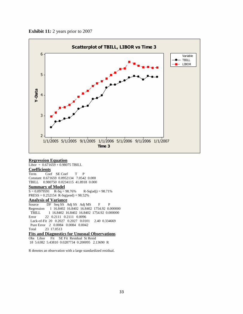
. It can be noted that in the years prior to 2007
the correlation was very similar to what it had been previously, i.e. 2005-2007 holds an R2 value
of 98.76% (Exhibit 11). Additionally, the 5 years leading up to 2008 represent an R2 value of
96.70%, which is also statistically speaking very high and significant considering the number of
39
Michaud, François-Louis, and Christian Upper. "What Drives Interbank Rates? Evidence from the Libor
Panel." What Drives Interbank Rates? Evidence from the Libor Panel. N.p., 3 Mar. 2008. 40
Smith, Yves. "Are Central Banks Making Libor WORSE?" Naked Capitalism RSS. N.p., 11 Oct. 2008. 41
Gaffen, David. "Libor, Damned Libor, and Statistics." MarketBeat RSS. N.p., 18 Sept. 2008. 42
Mollenkamp, Carrick, and Mark Whitehouse. "Study Casts Doubt on Key Rate; WSJ Analysis Suggests Banks
may have Reported Flawed Interest Data for Libor." Wall Street Journal: A.1.
Page 17
16
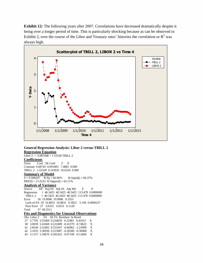
points observed (Exhibit 13). However, past 2007 and into 2008 through the present, the Libor
and the Treasuries diverged significantly; the ensuing R2 valued dropped to 66.96% from the
year 2008 to the present. Again, as compared to the previous years, this trend is dramatically
different from the one that was once observed by traders and the financial markets (Exhibit 12).
Over the course of any other 5 year period the Libor and the Treasury rates rose and fell at the
same pace, keeping high correlations to each other.
Conclusion
Over the past 22 years, the Libor and the Treasury rates have performed in tandem with
each other. The high statistical correlations during the boom and bust cycles have traditionally
remained very high giving credence to the argument that the two would perform similarly well
into the future. However, as it was seen through the analysis, the Libor rate had diverged
significantly from its previous correlations. The hypothesis that the two rates were highly
correlated remains true but only when the rates to the BBA are reported truthfully and honestly
and when there is a reasonable level certainty unlike during the late 1990s currency upheaval.
The divergence of the Libor rate during the scandal during the most recent financial crisis
therefore clearly showed that the rates were being tampered with. With both hindsight and
statistical analysis it is clear that the banks had acted in a collusive way that would prevent the
world from truly understanding how bad they were doing in during the financial crisis of 2008.
From the analysis, it is clear that the US Treasury was a good benchmark to use when examining
the Libor rate. However, in light of recent events, the comparison may no longer hold the same
significance or weight as previous understood. Until further regulation and policies are adopted
the BBA’s Libor rate cannot be fully trusted. We would adamantly state that until all of the
BBA’s reporting banks are closely examined, investors should be cautious of using this rate. But
Page 18
17
just as in many things, when there is a will to find shortcuts there will be both a way and
someone looking to exploit it.
Page 19
18
References _________________________________
"Banking Overview;British Bankers' Association." The Times: 1. Jan 23 1995. ProQuest
Central. Web. 27 Nov. 2012 .
"BBA Libor - The Basics." BbaLibor.com. BBA Libor, n.d. Web. 29 Nov. 2012.
<http://www.bbaLibor.com/bbaLibor-explained/the-basics>.
"Biz/ed - Correlation Explained [TimeWeb] | Biz/ed." Biz/ed - Correlation Explained
[TimeWeb] | Biz/ed. N.p., 2 Nov. 2002. Web. 02 Dec. 2012.
<http://www.bized.co.uk/timeweb/crunching/crunch_relate_expl.htm>.
"Dot.Com to Dot.Bomb." BBC News. BBC, 15 Dec. 2000. Web. 01 Dec. 2012.
<http://news.bbc.co.uk/2/hi/in_depth/business/2000/review/1069169.stm>.
Eade, Philip. "Minos Zombanakis." Euromoney.358 (1999): 24-. ProQuest Central. Web. 27
Nov. 2012. <http://search.proquest.com.ezproxy.babson.edu/docview/198853343>
Farrel, Maureen. "Explaining the Libor Interest Rate Mess." CNNMoney. Cable News Network,
03 July 2012. Web. 30 Nov. 2012. <http://money.cnn.com/2012/07/03/investing/Libor-
interest-rate-faq/index.htm>.
Finch, Gavin, and Anna Rascouet. "- Bloomberg." - Bloomberg. N.p., 14 Apr. 2009. Web. 01
Dec. 2012. http://www.bloomberg.com/apps/news?pid=newsarchive
Gaffen, David. "Libor, Damned Libor, and Statistics." MarketBeat RSS. N.p., 18 Sept. 2008.
Web. 01 Dec. 2012. <http://blogs.wsj.com/marketbeat/2008/09/18/Libor-damned-Libor-
and-statistics/>.
Hamour, Elwaleed A. "Initial Implications of the Introduction of the European Common
Currency "The Euro" for the Economies of the OIC Countries."Http://www.sesric.org/.
Journal of Economic Cooperation, 21 Jan. 2000. Web. 29 Nov. 2012.
<http://www.sesric.org/files/article/182.pdf >.
John Authers, Investment Editor. "Libor Rates." FT.com (2008): 1. ProQuest Central. Web. 27
Nov. 2012. <http://search.proquest.com.ezproxy.babson.edu/docview/229118837>
Madslien, Jorn. "Dotcom Bubble Burst: 10 Years on." BBC News. BBC, 03 Sept. 2010. Web. 01
Dec. 2012. <http://news.bbc.co.uk/2/hi/business/8558257.stm>.
Michaud, François-Louis, and Christian Upper. "What Drives Interbank Rates? Evidence from
the Libor Panel." What Drives Interbank Rates? Evidence from the Libor Panel. N.p., 3
Mar. 2008. Web. 01 Dec. 2012. <http://www.bis.org/publ/qtrpdf/r_qt0803f.htm>.
Page 20
19
Mollenkamp, Carrick, and Mark Whitehouse. "Study Casts Doubt on Key Rate; WSJ Analysis
Suggests Banks may have Reported Flawed Interest Data for Libor." Wall Street Journal:
A.1. ProQuest Central. May 29 2008. Web. 1 Dec. 2012 .
Pesek, William,Jr, and Xander Mellish. "Treasurys Finish Narrowly Mixed as the Dollar
Remains the Focus in Lieu of Other Indicators." Wall Street Journal: 0. ProQuest
Central. Mar 24 1995. Web. 1 Dec. 2012 .
http://search.proquest.com.ezproxy.babson.edu/docview/398451963/13AB01D89DA23D
7CACF/2?accountid=36796
"RELEASE: Pr6289-12." CFTC Orders Barclays to Pay $200 Million Penalty for Attempted
Manipulation of and False Reporting concerning LIBOR and Euribor Benchmark Interest
Rates. U.S. Commodity Futures Trading Commission, 27 June 2012. Web. 30 Nov. 2012.
<http://www.cftc.gov/PressRoom/PressReleases/pr6289-12>.
Ridley, Kirstin, and Huw Jones. "A Greek Banker Spills On The Early Days Of The Libor And
His First Deal With The Shah Of Iran." Www.BusinessInsider.com. Business Insider, 8
Aug. 2012. Web. 27 Nov. 2012. <http://www.businessinsider.com/history-of-the-Libor-
rate-2012-8>.
Saunders, Anthony, and Marcia M. Cornett. Financial Markets and Institutions: A Modern
Perspective. 5th ed. N.p.: Irwin/McGraw-Hill, 2012. Print.
SHEEL KOHLI, in L. "US Trade Relations Tested as Japan Warns of Strict Measures to Stem
Currency's Fall Nuclear Fallout Hurts Yen." South China Morning Post: 1. ProQuest
Central. May 30 1998. Web. 1 Dec. 2012 .
http://search.proquest.com.ezproxy.babson.edu/docview/265436666/13AB26E55FD7DD
CDE8B/3?accountid=36796
Smith, Yves. "Are Central Banks Making Libor WORSE?" Naked Capitalism RSS. N.p., 11 Oct.
2008. Web. 01 Dec. 2012. <http://www.nakedcapitalism.com/2008/10/are-central-banks-
making-Libor-worse.html>.
Staff, and Agencies. "Ben Bernanke and Mervyn King Describe Libor Fixing as 'fraud'" The
Guardian. Guardian News and Media, 17 July 2012. Web. 02 Dec. 2012.
<http://www.guardian.co.uk/business/2012/jul/17/federal-reserve-ben-bernanke>.
"Syndicated Loan." Investopedia.com. Investopedia, n.d. Web. 29 Nov. 2012.
<http://www.investopedia.com/terms/s/syndicatedloan.asp>.
Taaffe, Ouida. "The Life and Good times of Libor." - Minos Zombanakis. IFS School of Finance,
n.d. Web. 29 Nov. 2012.
<http://fw.ifslearning.ac.uk/Archive/2012/June/Features/ThelifeandgoodtimesofLibormin
oszombanakis.aspx>.
Page 21
20
"Timeline: Libor-fixing Scandal." BBC News. BBC, 26 Sept. 2012. Web. 30 Nov. 2012.
<http://www.bbc.co.uk/news/business-18671255>.
"The Dot-Com Bubble Bursts." The New York Times. The New York Times, 24 Dec. 2000. Web.
01 Dec. 2012. <http://www.nytimes.com/2000/12/24/opinion/the-dot-com-bubble-
bursts.html>.
Page 22
21
Appendix
Exhibit 1
(Source: Mollenkamp, Carrick, and Mark Whitehouse. "Study Casts Doubt on Key Rate;
WSJ Analysis Suggests Banks may have Reported Flawed Interest Data for LIBOR." Wall
Street Journal: A.1. ProQuest Central. May 29 2008.)
Page 23
22
Exhibit 2: All data points were considered in this graph. Data was collected from the beginning
of the Libor Rate to the present as well as all of the data for the Treasury bills. All data used in
this Exhibit as well as the following will be based off of the 6 month rates for both rates.
1/1/20151/1/20101/1/20051/1/20001/1/19951/1/1990
9
8
7
6
5
4
3
2
1
0
ALL
Y-D
ata
Tbill 6m
6 month Libor
Variable
Scatterplot of Tbill 6m, 6 month Libor vs ALL
General Regression Analysis: Tbill 6m versus 6 month Libor
Regression Equation Tbill 6m = -0.471649 + 0.944927 6 month Libor
Coefficients Term Coef SE Coef T P
Constant -0.471649 0.0478600 -9.8548 0.000
6 month Libor 0.944927 0.0102709 92.0005 0.000
Summary of Model S = 0.392567 R-Sq = 96.84% R-Sq(adj) = 96.83%
PRESS = 43.0095 R-Sq(pred) = 96.81%
Analysis of Variance Source DF Seq SS Adj SS Adj MS F P
Regression 1 1304.39 1304.39 1304.39 8464.09 0.0000000
6 month Libor 1 1304.39 1304.39 1304.39 8464.09 0.0000000
Error 276 42.53 42.53 0.15
Lack-of-Fit 246 41.71 41.71 0.17 6.15 0.0000001
Pure Error 30 0.83 0.83 0.03
Total 277 1346.92
Fits and Diagnostics for Unusual Observations Obs Tbill 6m Fit SE Fit Residual St Resid
217 3.70 4.58730 0.0270514 -0.88730 -2.26564 R
219 3.07 4.09462 0.0248554 -1.02462 -2.61529 R
220 3.14 4.08762 0.0248311 -0.94762 -2.41876 R
221 1.87 3.09970 0.0237164 -1.22970 -3.13820 R
223 1.27 2.06057 0.0274664 -0.79057 -2.01878 R
224 1.34 2.21062 0.0266632 -0.87062 -2.22290 R
Page 24
23
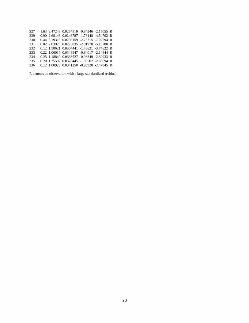
227 1.63 2.47246 0.0254519 -0.84246 -2.15055 R
229 0.90 2.68148 0.0246787 -1.78148 -4.54702 R
230 0.44 3.19315 0.0236159 -2.75315 -7.02594 R
231 0.02 2.03978 0.0275835 -2.01978 -5.15780 R
232 0.12 1.58621 0.0304441 -1.46621 -3.74622 R
233 0.22 1.06017 0.0343547 -0.84017 -2.14844 R
234 0.25 1.18849 0.0333527 -0.93849 -2.39933 R
235 0.20 1.25502 0.0328445 -1.05502 -2.69694 R
236 0.12 1.08928 0.0341250 -0.96928 -2.47845 R
R denotes an observation with a large standardized residual.
Page 25
24
Exhibit 3: In this data set we observed the Libor vs the Treasury using only data that occurred
before the 217th
data point, or in terms of dates, August 2007. We conducted this analysis to
show that the R2 value was higher before this time frame and that the unusual observations were
in fact unusual.
1/1/20101/1/20051/1/20001/1/19951/1/1990
9
8
7
6
5
4
3
2
1
0
Time
Y-D
ata
6 m Tbill
6 month Libor
Variable
Scatterplot of 6 m Tbill, 6 month Libor vs Time
General Regression Analysis: 6 month Libor versus 6 m Tbill
Regression Equation 6 month Libor = 0.218341 + 1.09934 6 m Tbill
Coefficients Term Coef SE Coef T P
Constant 0.21834 0.0379692 5.750 0.000
6 m Tbill 1.09934 0.0083958 130.940 0.000
Summary of Model S = 0.214849 R-Sq = 98.77% R-Sq(adj) = 98.76%
PRESS = 10.0490 R-Sq(pred) = 98.75%
Analysis of Variance Source DF Seq SS Adj SS Adj MS F P
Regression 1 791.429 791.429 791.429 17145.3 0.000000
6 m Tbill 1 791.429 791.429 791.429 17145.3 0.000000
Error 214 9.878 9.878 0.046
Lack-of-Fit 162 7.830 7.830 0.048 1.2 0.197857
Pure Error 52 2.049 2.049 0.039
Total 215 801.307
Fits and Diagnostics for Unusual Observations 6 month
Obs Libor Fit SE Fit Residual St Resid
15 8.3750 7.93573 0.0280130 0.439268 2.06215 R
58 5.2500 4.76962 0.0146214 0.480377 2.24108 R
64 7.0000 6.29771 0.0185298 0.702290 3.28099 R
93 6.0080 5.51718 0.0155929 0.490824 2.29055 R
Page 26
25
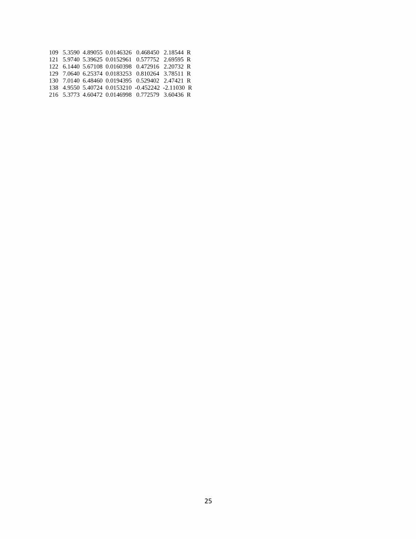
109 5.3590 4.89055 0.0146326 0.468450 2.18544 R
121 5.9740 5.39625 0.0152961 0.577752 2.69595 R
122 6.1440 5.67108 0.0160398 0.472916 2.20732 R
129 7.0640 6.25374 0.0183253 0.810264 3.78511 R
130 7.0140 6.48460 0.0194395 0.529402 2.47421 R
138 4.9550 5.40724 0.0153210 -0.452242 -2.11030 R
216 5.3773 4.60472 0.0146998 0.772579 3.60436 R
Page 27
26
Exhibit 4
1/1/19951/1/19941/1/19931/1/19921/1/19911/1/1990
9
8
7
6
5
4
3
2
90-94
Y-D
ata
6m Tbill
6m LIBOR
Variable
Scatterplot of 6m Tbill, 6m LIBOR vs 90-94
Page 28
27
Exhibit 5
1.41.21.00.80.60.40.2
12
10
8
6
4
2
0
1990-1994 Spread
Fre
qu
en
cy
Mean 0.7011
StDev 0.2640
N 60
Histogram of 1990-1994 SpreadNormal
Page 29
28
Exhibit 6
1/1/20001/1/19991/1/19981/1/19971/1/19961/1/1995
7.0
6.5
6.0
5.5
5.0
4.5
4.0
95-99
Y-D
ata
6m Tbill_1
6m LIBOR_1
Variable
Scatterplot of 6m Tbill_1, 6m LIBOR_1 vs 95-99
Page 30
29
Exhibit 7
1.21.00.80.60.4
12
10
8
6
4
2
0
1995-1999 Spread
Fre
qu
en
cy
Mean 0.7669
StDev 0.2097
N 60
Histogram of 1995-1999 SpreadNormal
Page 31
30
Exhibit 8: From the beginning of 2000 through 2004, the markets had just experienced a major
collapse of the technology and dot come bubble. The following result shows both of the rates
decreasing. But towards the end of this time frame, the global economy was on the rise and the
United States in particular was gaining traction for the housing bubble.
1/1/20051/1/20041/1/20031/1/20021/1/20011/1/2000
7
6
5
4
3
2
1
0
00-04
Y-D
ata
6m Tbill_2
6m LIBOR_2
Variable
Scatterplot of 6m Tbill_2, 6m LIBOR_2 vs 00-04
General Regression Analysis: 6m Tbill_2 versus 6m Libor_2
Regression Equation 6m Tbill_2 = -0.123156 + 0.899559 6m Libor_2
Coefficients Term Coef SE Coef T P
Constant -0.123156 0.0420073 -2.9318 0.005
6m Libor_2 0.899559 0.0114493 78.5688 0.000
Summary of Model S = 0.182084 R-Sq = 99.07% R-Sq(adj) = 99.05%
PRESS = 2.13872 R-Sq(pred) = 98.96%
Analysis of Variance Source DF Seq SS Adj SS Adj MS F P
Regression 1 204.664 204.664 204.664 6173.06 0
6m Libor_2 1 204.664 204.664 204.664 6173.06 0
Error 58 1.923 1.923 0.033
Total 59 206.587
Fits and Diagnostics for Unusual Observations 6m
Obs Tbill_2 Fit SE Fit Residual St Resid
5 5.49 6.23133 0.0517149 -0.741331 -4.24624 R
6 5.70 6.18635 0.0512057 -0.486353 -2.78337 R
14 4.72 4.33416 0.0321392 0.385840 2.15283 R
R denotes an observation with a large standardized residual.
Page 32
31
Exhibit 9: In this chart it can be observed that the spread between the two rates became
dramatically larger after mid-2007.
0
0.5
1
1.5
2
2.5
3
3.5
4
8/1/20042/17/20059/5/20053/24/200610/10/20064/28/200711/14/20076/1/200812/18/20087/6/20091/22/20108/10/2010
Rat
e
6 Month Libor and Treasury Rate Spread
Page 33
32
Exhibit 10: 2005 through 2009 shows the bottom of the market as well as the peak. This data
represents 2 very different environments of the global economy as well as the domestic UK and
USA.
1/1/20101/1/20091/1/20081/1/20071/1/20061/1/2005
6
5
4
3
2
1
0
05-09
Y-D
ata
6m Tbill_3
6m LIBOR_3
Variable
Scatterplot of 6m Tbill_3, 6m LIBOR_3 vs 05-09
General Regression Analysis: 6m Tbill_3 versus 6m Libor_3
Regression Equation 6m Tbill_3 = -1.28095 + 1.07721 6m Libor_3
Coefficients Term Coef SE Coef T P
Constant -1.28095 0.201783 -6.3482 0.000
6m Libor_3 1.07721 0.049880 21.5959 0.000
Summary of Model S = 0.621018 R-Sq = 88.94% R-Sq(adj) = 88.75%
PRESS = 23.7717 R-Sq(pred) = 88.25%
Analysis of Variance Source DF Seq SS Adj SS Adj MS F P
Regression 1 179.867 179.867 179.867 466.383 0
6m Libor_3 1 179.867 179.867 179.867 466.383 0
Error 58 22.369 22.369 0.386
Total 59 202.236
Fits and Diagnostics for Unusual Observations 6m
Obs Tbill_3 Fit SE Fit Residual St Resid
45 0.90 2.31360 0.0823309 -1.41360 -2.29653 R
46 0.44 2.89691 0.0806000 -2.45691 -3.99001 R
47 0.02 1.58207 0.0958876 -1.56207 -2.54586 R
R denotes an observation with a large standardized residual.
Page 34
33
Exhibit 11: 2 years prior to 2007
1/1/20079/1/20065/1/20061/1/20069/1/20055/1/20051/1/2005
6
5
4
3
2
Time 3
Y-D
ata
TBILL
LIBOR
Variable
Scatterplot of TBILL, LIBOR vs Time 3
Regression Equation Libor = 0.671659 + 0.98075 TBILL
Coefficients Term Coef SE Coef T P
Constant 0.671659 0.0952134 7.0542 0.000
TBILL 0.980750 0.0234115 41.8918 0.000
Summary of Model S = 0.0979591 R-Sq = 98.76% R-Sq(adj) = 98.71%
PRESS = 0.252154 R-Sq(pred) = 98.52%
Analysis of Variance Source DF Seq SS Adj SS Adj MS F P
Regression 1 16.8402 16.8402 16.8402 1754.92 0.000000
TBILL 1 16.8402 16.8402 16.8402 1754.92 0.000000
Error 22 0.2111 0.2111 0.0096
Lack-of-Fit 20 0.2027 0.2027 0.0101 2.40 0.334669
Pure Error 2 0.0084 0.0084 0.0042
Total 23 17.0513
Fits and Diagnostics for Unusual Observations Obs Libor Fit SE Fit Residual St Resid
18 5.6382 5.43810 0.0287734 0.200095 2.13690 R
R denotes an observation with a large standardized residual.
Page 35
34
Exhibit 12: The following years after 2007. Correlations have decreased dramatically despite it
being over a longer period of time. This is particularly shocking because as can be observed in
Exhibit 2, over the course of the Libor and Treasury rates’ histories the correlation or R2 was
always high.
1/1/20131/1/20121/1/20111/1/20101/1/20091/1/2008
4
3
2
1
0
Time 4
Y-D
ata
TBILL 2
LIBOR 2
Variable
Scatterplot of TBILL 2, LIBOR 2 vs Time 4
General Regression Analysis: Libor 2 versus TBILL 2
Regression Equation Libor 2 = 0.687448 + 1.53328 TBILL 2
Coefficients Term Coef SE Coef T P
Constant 0.68745 0.091805 7.4881 0.000
TBILL 2 1.53328 0.143935 10.6526 0.000
Summary of Model S = 0.596247 R-Sq = 66.96% R-Sq(adj) = 66.37%
PRESS = 21.0233 R-Sq(pred) = 65.11%
Analysis of Variance Source DF Seq SS Adj SS Adj MS F P
Regression 1 40.3425 40.3425 40.3425 113.478 0.0000000
TBILL 2 1 40.3425 40.3425 40.3425 113.478 0.0000000
Error 56 19.9086 19.9086 0.3555
Lack-of-Fit 29 16.8833 16.8833 0.5822 5.196 0.0000237
Pure Error 27 3.0253 3.0253 0.1120
Total 57 60.2511
Fits and Diagnostics for Unusual Observations Obs Libor 2 Fit SE Fit Residual St Resid
37 3.7795 3.55469 0.234659 0.22481 0.41015 X
38 3.0039 3.41669 0.222489 -0.41279 -0.74622 X
41 2.8544 3.52402 0.231947 -0.66962 -1.21909 X
42 3.1035 3.30936 0.213087 -0.20586 -0.36968 X
43 3.1157 3.18670 0.202422 -0.07100 -0.12660 X
Page 36
35
44 3.1116 3.27870 0.210413 -0.16710 -0.29952 X
45 3.3369 2.06740 0.113082 1.26950 2.16851 R
46 3.8784 1.36209 0.079789 2.51631 4.25855 R
47 2.6578 0.71811 0.090335 1.93969 3.29115 R
48 2.1778 0.87144 0.084085 1.30636 2.21309 R
R denotes an observation with a large standardized residual.
X denotes an observation whose X value gives it large leverage.
Page 37
36
Exhibit 13:
1/1/20081/1/20071/1/20061/1/20051/1/20041/1/2003
6
5
4
3
2
1
Time 3
Y-D
ata
TBILL
LIBOR
Variable
Scatterplot of TBILL, LIBOR vs Time 3
General Regression Analysis: Libor versus TBILL
Regression Equation Libor = 0.306616 + 1.08948 TBILL
Coefficients Term Coef SE Coef T P
Constant 0.30662 0.0877202 3.4954 0.001
TBILL 1.08948 0.0264312 41.2194 0.000
Summary of Model S = 0.319572 R-Sq = 96.70% R-Sq(adj) = 96.64%
PRESS = 6.22133 R-Sq(pred) = 96.53%
Analysis of Variance Source DF Seq SS Adj SS Adj MS F P
Regression 1 173.516 173.516 173.516 1699.04 0.0000000
TBILL 1 173.516 173.516 173.516 1699.04 0.0000000
Error 58 5.923 5.923 0.102
Lack-of-Fit 48 5.898 5.898 0.123 49.25 0.0000001
Pure Error 10 0.025 0.025 0.002
Total 59 179.439
Fits and Diagnostics for Unusual Observations Obs Libor Fit SE Fit Residual St Resid
56 5.3773 4.65364 0.0498878 0.72366 2.29258 R
57 5.3538 4.33769 0.0460170 1.01611 3.21308 R
59 4.8324 3.65132 0.0414249 1.18108 3.72727 R
60 4.8250 3.72758 0.0416324 1.09742 3.46354 R
R denotes an observation with a large standardized residual.