Long run evidence on money growth and inflation · by Luca Benati Long Run EvidEncE on MonEy gRowth...

by Luca Benati

Long Run EvidEncE on MonEy gRowth and infLation

woRk ing PaPER SER i E Sno 1027 / MaRch 2009

WORKING PAPER SER IESNO 1027 / MARCH 2009

This paper can be downloaded without charge fromhttp://www.ecb.europa.eu or from the Social Science Research Network

electronic library at http://ssrn.com/abstract_id=1345758.

In 2009 all ECB publications

feature a motif taken from the

€200 banknote.

LONG RUN EVIDENCE ON MONEY

GROWTH AND INFLATION 1

by Luca Benati 2

1 I wish to thank M. Canzoneri, C. Goodhart, G. Lombardo, E. Nelson, S. Reynard, M. Rostagno, and M. Woodford for helpful discussions, and

seminar participants at the Bank of England for comments on an earlier draft. Special thanks to C. Close and J. Holloway, and to

S. Reynard, for kindly providing the long-run data for Australia, and Switzerland, respectively; to A. Baffigi and J.-P. Cayen

for providing the monthly post-WWII series for Italy and Canada, respectively; and to J. Hassler for allowing me

to use his long-run dataset for Sweden. The views expressed in this paper are those of the author and

do not necessarily reflect those of the European Central Bank.

2 Monetary Policy Strategy Division, European Central Bank, Kaiserstrasse 29, D-60311, Frankfurt am Main, Germany;

e-mail: [email protected]

© European Central Bank, 2009

Address Kaiserstrasse 29 60311 Frankfurt am Main, Germany

Postal address Postfach 16 03 19 60066 Frankfurt am Main, Germany

Telephone +49 69 1344 0

Website http://www.ecb.europa.eu

Fax +49 69 1344 6000

All rights reserved.

Any reproduction, publication and reprint in the form of a different publication, whether printed or produced electronically, in whole or in part, is permitted only with the explicit written authorisation of the ECB or the author(s).

The views expressed in this paper do not necessarily refl ect those of the European Central Bank.

The statement of purpose for the ECB Working Paper Series is available from the ECB website, http://www.ecb.europa.eu/pub/scientific/wps/date/html/index.en.html

ISSN 1725-2806 (online)

3ECB

Working Paper Series No 1027March 2009

Abstract 4

Non-technical summary 5

1 Introduction 6

1.1 Main results 6

1.2 Interpreting the results 7

2 Lucas (1980) Redux: evidence from band-pass fi ltering 8

3 Evidence from cross-spectral methods 10

3.1 Methodology 10

3.2 Empirical evidence 12

4 Interpreting the evidence 19

4.1 The impact of monetary policy 19

4.2 Velocity shocks and infrequent infl ationary outbursts 21

4.3 Two further ‘non-explanations’ 26

5 Conclusions 27

References 29

Annex: The Data 34

Tables and fi gures 40

European Central Bank Working Paper Series 79

CONTENTS

4ECBWorking Paper Series No 1027March 2009

Abstract Over the last two centuries, the cross-spectral coherence between either narrow or broad money growth and inflation at the frequency ω=0 has exhibited little variation–being, most of the time, close to one–in the U.S., the U.K., and several other countries, thus implying that the fraction of inflation’s long-run variation explained by long-run money growth has been very high and relatively stable. The cross-spectral gain at ω=0, on the other hand, has exhibited significant changes, being for long periods of time smaller than one. The unitary gain associated with the quantity theory of money appeared in correspondence with the inflationary outbursts associated with World War I and the Great Inflation–but not World War II–whereas following the disinflation of the early 1980s the gain dropped below one for all the countries and all the monetary aggregates I consider, with one single exception. I propose an interpretation for this pattern of variation based on the combination of systematic velocity shocks and infrequent inflationary outbursts. Based on estimated DSGE models, I show that velocity shocks cause, ceteris paribus, comparatively much larger decreases in the gain between money growth and inflation at ω=0 than in the coherence, thus implying that monetary regimes characterised by low and stable inflation exhibit a low gain, but a still comparatively high coherence. Infrequent inflationary outbursts, on the other hand, boost both the gain and coherence towards one, thus temporarily revealing the one-for-one correlation between money growth and inflation associated with the quantity theory of money, which would otherwise remain hidden in the data. Keywords: Quantity theory of money, inflation, frequency domain, cross-spectral analysis, band-pass filtering, DSGE models, Bayesian estimation, trend inflation. JEL Classification: E30, E32

Non-technical summary Over the last two centuries, the fraction of inflation’s long-run variation explained by

long-run money growth has been very high, and relatively stable, in the United States,

the United Kingdom and several other countries. The proportionality between the

long-run components of money growth and inflation, on the other hand, has exhibited

significant changes, being for long periods of time lower than one-for-one. In

particular, the one-for-one correlation between the long-run components of money

growth and inflation associated with the quantity theory of money appeared in

correspondence with the inflationary outbursts associated with World War I and the

Great Inflation, whereas following the disinflation of the early 1980s the correlation

dropped below one for all the countries and all the monetary aggregates considered

herein, with one single exception.

The paper proposes an interpretation for the identified stylised facts based on the

combination of systematic velocity shocks and infrequent inflationary outbursts.

Based on estimated structural macroeconomic models, it is shown that velocity

shocks cause, ceteris paribus, comparatively much larger decreases in the correlation

between the long-run components of money growth and inflation than in the fraction

of inflation’s variance explained by money growth. This implies that monetary

regimes characterised by low and stable inflation exhibit a low correlation between

the long-run components of the two series, whereas the fraction of inflation’s

variance explained by money growth is still comparatively high. Infrequent

inflationary outbursts, on the other hand, boost the correlation towards one, thus

temporarily revealing the one-for-one association between the long-run components

of money growth and inflation, which would otherwise remain hidden in the data.

5ECB


The central predictions of the quantity theory are that, in the long run, moneygrowth should be neutral in its effects on the growth rate of production, andshould affect the inflation rate on a one-for-one basis.

–R.E. Lucas, Jr.1

[...] think of velocity shocks as the noise that obscures the signal from monetaryaggregates. In a regime in which changes in [...] inflation and the money supplyare subdued, the signal-to-noise ratio is likely to be low [...]. However, in othereconomies or in other time periods in which we experience more pronounced chan-ges in money and inflation, the velocity shocks might become small relative tothe swings in money growth, thus producing a higher signal-to-noise ratio.

–A. Estrella and F.S. Mishkin2

1 Introduction

This paper is an investigation of the relationship between money growth and inflationat the very low frequencies over the last two centuries. Based on data for inflation andthe rates of growth of both narrow and broad monetary aggregates for the UnitedStates, the United Kingdom, and several other countries since the Gold Standard era,I use frequency-domain techniques to address the following questions.

(1) ‘In the very long run–which I identify with the frequency ω=0–do moneygrowth and inflation move one-for-one, as predicted by the quantity theory of money?’(2) ‘What is the fraction of long-run–i.e., frequency-zero–inflation variance

which is explained by long-run money growth?’(3) ‘Are the relationships identified in (1) and (2) stable over time? And if the an-

swer is ‘No’, have they historically exhibited any systematic pattern of time-variation?’

1.1 Main results

I document several facts. In particular,

• over the last two centuries the cross-spectral gain between either narrow orbroadmoney growth and inflation at the frequency ω=0 has exhibited importantchanges in most countries, and it has been, for long periods of time, significantlysmaller than one at conventional levels. Taken at face value, this result impliesthat, for long periods of time, the long-run component of inflation has movedless than one-for-one with the long-run component of money growth.

1See Lucas (1995).2See Estrella and Mishkin (1997).


• The cross-spectral coherence between the two series, on the other hand, hasexhibited much less variation, and it has been, most of the times, close to one,thus implying that the fraction of inflation’s long-run variation explained bylong-run money growth has consistently been close to 100 per cent.

• Evidence for the United States and the United Kingdom (the only two coun-tries for which high-frequency data for both money and prices are available sincebefore World War I) suggests that the unitary gain at ω=0 conceptually asso-ciated with the quantity theory of money appeared in correspondence with theinflationary upsurges associated with World War I and the Great Inflation–butnot World War II.3 Following the disinflation of the early 1980s, the gain atzero dropped below one for all the countries and all the monetary aggregates Iconsider, with the single exception of M3 for Sweden.

• Finally, a comparison between the pre-1914 metallic standard era and the post-WWII period suggests that Rolnick and Weber’s (1997) key finding–basedon the raw data–of a weaker correlation between money growth and inflationunder metallic than under fiat standards also holds, most of the times, for thelow-frequency components of the two series.

1.2 Interpreting the results

Conceptually in line with Estrella and Mishkin (1997), I propose an interpretationfor the identified pattern of variation in the gain and the coherence at ω=0 based onthe combination of systematic velocity shocks, and infrequent inflationary upsurgesdue to either policy mistakes or major geo-political upheavals. Based on estimatedDSGE models, I show that velocity shocks cause, ceteris paribus, comparatively muchlarger decreases in the gain between money growth and inflation at ω=0 than in thecoherence, so that monetary regimes characterised by low and stable inflation exhibit,in general, a low gain, but a still comparatively high coherence. On the other hand,infrequent inflationary upsurges–such as those associated with World War I and theGreat Inflation–by ‘swamping’ the velocity growth noise away, temporarily revealthe one-for-one long-run relationship between the two series, which would otherwiseremain hidden in the data.I also show that three alternative mechanisms which–at least in principle–might

account for the identified pattern of variation, do not offer satisfactory explanations.Specifically, first, I show that changes in monetary policy have a hard time in repro-ducing the identified pattern of variation. Indeed, on the one hand, under determinacyboth the gain and the coherence at zero are largely invariant to changes in the sys-tematic component of monetary policy. On the other hand, indeterminacy is typically

3As I discuss in Section 3.2.3, the most logical explanation for the different pattern between WWIand WWII is the presence of extensive price controls during the latter conflict, but not during theformer.

7ECB


associated with lower values of both the gain and the coherence, thus implying that(i) this explanation would still fail to account for the different pattern of variation inthe two cross-spectral statistics, and (ii) it would crucially hinge on the notion thatcomparatively more stable monetary regimes–such as the Gold Standard, or theperiod following the disinflation of the first half of the 1980s–are characterised byindeterminacy, whereas during periods such as the Great Inflation the economy wasunder determinacy, which most macroeconomists would most likely find unappealing.Second, in line with Lucas (1988) and Reynard (2006), I explore the possibility

that a gain at zero lower than one may result from systematic, endogenous shiftsin velocity growth due to Fisherian movements in interest rates–and therefore, inthe opportunity cost of money–caused by shifts in the low-frequency (and there-fore, highly predictable) component of inflation. This mechanism, too, appears asincapable of explaining the pattern of variation seen in the data.Third, I show that changes in the elasticity of money demand with respect to

either output or the interest rate has essentially no impact on either the gain or thecoherence at ω=0.

The paper is organised as follows. The next section presents, in the spirit of Lucas’(1980) classic analysis of the low-frequency association between money growth andinflation, evidence from band-pass filtering. Section 3 presents evidence from cross-spectral analysis, whereas Section 4 discusses several possible explanations for ourfindings. Section 5 concludes.

2 Lucas (1980) Redux : Evidence from Band-PassFiltering

In ‘Two Illustrations of the Quantity Theory of Money’, Robert Lucas used linearfiltering techniques4 to extract low-frequency components from U.S. M1 growth andCPI inflation over the period 1955-1975, uncovering a near one-for-one correlationbetween the two series at the very low frequencies.5 He interpreted his evidence as

‘[...] additional confirmation of the quantity theory, as an example ofone way in which the quantity-theoretic relationships can be recoveredvia atheoretical methods from time-series which are subject to a varietyof other forces [...].’

Figure 1 shows some of the series in our dataset, which is described in detail inAppendix A. Figure 2 presents evidence in the spirit of Lucas (1980), by plotting, for

4Specifically, a ‘precursor’ of the Hodrick-Prescott filter.5As I will discuss more extensively in Section 3.2.1, however, McCallum (1984), and especially

Whiteman (1984), pointed out how Lucas’ results, being based on reduced-form methods, were inprinciple vulnerable to the Lucas (1976) critique, and as such they could not be interpreted asevidence in favor of the quantity theory of money.


the series shown in Figure 1, the components of broad money growth and inflationwith a frequency of oscillation beyond 30 years.6 The approximated band-pass filterwe use in order to extract the low-frequency components from the raw data is theone proposed by Christiano and Fitzgerald (2003).7 Consistent with the evidencereported in Lucas (1980), Figure 2 points towards a very close correlation betweenthe low-frequency components of broad money growth and inflation since the metallicstandards era. Evidence appears especially strong for the United States, Norway, theUnited Kingdom, Australia, and Portugal–for which the ‘eyeball metric’ suggests thecorrelation to be very close to one-for-one–less so for the remaining countries, andin particular for Switzerland, Italy, and the Netherlands, for which the low-frequencycomponents of the two series appear to sometimes diverge to a non-negligible extent.How should we interpret these results? At first sight, the fact that the correla-

tion between money growth and inflation at the very low frequencies appears to haveremained stable across such a marked variation in monetary arrangements over thelast two centuries–from a de jure or de facto Gold Standard, to, in most cases,de jure or de facto inflation targeting–seems to suggest that such correlation isindeed structural in the sense of Lucas (1976), and it is therefore ‘hardwired’ intothe deep structure of the economy.8 A crucial problem with this kind of evidence,however, is that strictly speaking band-pass filtering (or, more generally, linear fil-tering) is not a proper econometric method, in the sense that–different from, e.g.,cross-spectral analysis–it does not provide numerical estimates, and measures of un-certainty around such estimates, for key objects of interest capturing the relationshipbetween the two series. As a result, even evidence at first sight strong–such as thatfor the United States or Norway–ought necessarily to be regarded as purely sug-gestive of stable relationship between money growth and inflation at the very lowfrequencies since the metallic standard era.In the next section we therefore turn to cross-spectral methods, which will allow us

to compute precise numerical estimates of key objects of interest, and–crucially–to

6A legitimate question is: ‘Why choosing 30 years as the lower bound of the frequency band ofinterest?’ To be fair, there is no compelling reason why 30 years should be preferred to, say, 29 or37. Christiano and Fitzgerald (2003, Section 5), for example, consider three frequency bands, withthe lowest frequencies being associated with fluctuations between 20 and 40 years.

7To be precise, for a sample of size T , Christiano and Fitzgerald (2003) provide formulas forfiltered observations from t=3 to t=T -2, thus losing 2 observations at the beginning and 2 at theend of the sample. I worked out the formulas for the first two and the last two observations, sothat in performinng band-pass filtering I do not lose any observation. (Needless to say, because ofend-of-sample problems, these additional observations are filtered quite imprecisely.)

8To the very best of my knowledge, this argument was first made by Batini and Nelson (2002)based on the analysis of raw U.K. and U.S. data since the Gold Standard. As discussed in Batini andNelson (2002), Friedman (1961) originally made the conceptually related argument that ‘[f ]or theUnited States for nearly a century [...] cyclical movements in money have apparently had much thesame relation in both timing and amplitude to cyclical movements in business under very differentmonetary arrangements, though of course the movements in money or in business alone have beenvery different’.

9ECB


characterise the extent of econometric uncertainty associated with such estimates.

3 Evidence from Cross-Spectral Methods

3.1 Methodology

3.1.1 Computing cross-spectral objects

Let xt and yt be two jointly covariance-stationary series, with xt being the ‘input’series (in the language of transfer function models), and yt being the ‘output’ series(in our case, xt and yt are money growth and, respectively, inflation); let Fx(ωj) andFy(ωj) be the smoothed spectra of the two series at the Fourier frequency ωj; andlet Cx,y(ωj) and Qx,y(ωj) be the smoothed co-spectrum and, respectively, quadraturespectrum between xt and yt at the Fourier frequency ωj. We estimate both the spectraldensities of xt and yt, the co-spectrum, and the quadrature spectrum, by smoothingthe periodograms and, respectively, the cross-periodogram in the frequency domain bymeans of a Bartlett spectral window. We select the spectral bandwidth automaticallyvia the procedure proposed by Beltrao and Bloomfield (1987). For a specific Fourierfrequency ωj, the estimated smoothed gain and coherence9 are then defined as10

Γ(ωj) =[Cx,y(ωj)

2 +Qx,y(ωj)2]

12

Fx(ωj)(1)

K(ωj) =

½Cx,y(ωj)

2 +Qx,y(ωj)2

Fx (ωj) · Fy (ωj)

¾ 12

(2)

9On the other hand, we disregard the phase angle. There are several reasons for doing so. First,the interpretation of the phase angle statistic is intrinsically conceptually tricky, as we are deal-ing with sine and cosine waves. To illustrate the problem in the simplest possible way, does thesine lead the cosine, or vice-versa? Given that cos(ω)=sin(ω+π/2), it is conceptually impossibleto establish which of the two series leads the other one. Second, given that the phase angle is de-fined as P (ωj)=-arctan[Qx,y(ωj)/Cx,y(ωj)], and given that the tangent function is periodic, it istechnically impossible to compute confidence intervals for the phase statistics via spectral boot-strapping, as the arctangent function converts a sufficiently large bootstrapped realisation of theratio Qx,y(ωj)/Cx,y(ωj) into a comparatively small realisation of the phase, precisely because aftera certain threshold the periodicity kicks in. (An alternative would be to use asymptotic confidencebands, but based on my own experience–based on extensive Monte Carlo–they have, unsurpris-ingly, a very poor.coverage.)10It is to be noticed that the literature presents alternative, slightly different definitions of the

gain and the coherence–on this, see (e.g.) Hamilton (1994), page 275. The gain, for example, issometimes defined as the numerator of (1), whereas the coherence is defined as the square of (2).


3.1.2 Monte Carlo evidence on the performance of the cross-spectral es-timators

Since, ultimately, our results are only as reliable as our estimators, in this section wepresent some Monte Carlo evidence on the their performance conditional on a widelyrepresentative data generation process (henceforth, DGP). For three sample lenghts,T = 200, 500, 1000, we simulate N times (with N = 5,000) the following DGP:

xt = ρxxt−1 + ut + θuxut−1 + vt + θvxvt−1 (3)

yt = ρyyt−1 + ut + θuyut−1 + vt + θvyvt−1 (4)

with ut and vt unit-variance white noise.11 For each of the N simulations, we drawthe key parameters12–ρx, ρy, θux, θvx, θuy, and θvy–as follows. θux, θvx, θuy, and θvyare drawn from uniform distributions defined over [-0.5; 0.5].13 The AR parameters(ρx and ρy) on the other hand, are drawn from a uniform distribution defined over[0; 0.9]. For each single stochastic simulation we estimate the gain and the coherence,and we then compute the difference between the estimated objects and the theoreticalones, which we compute by Fourier-transforming the DGP conditional on the verysame random configuration of parameters, ρx, ρy, θux, θvx, θuy, and θvy which we usedto perform the simulation.Figure 3 shows the medians of the Monte Carlo distributions of the differences

between estimated and theoretical gains and coherences, together with the 90 percent lower and upper percentiles. As the figure clearly shows, the performance ofthe gain and coherence estimators is uniformly excellent, with the medians of thedistributions virtually flat at zero for all the three sample lengths, thus pointingtowards no systematic bias in either object at any frequency.

3.1.3 Computing confidence bands

We compute confidence bands via the non-parametric multivariate spectral bootstrapprocedure introduced by Berkowitz and Diebold (1998)–more precisely, via the firstof the two procedures they propose. As they show via Monte Carlo, such a proceduregenerates confidence intervals with superior coverage properties compared to thosebased on the approximated asymptotic formulas found for example in Koopmans(1974), ch. 8. The Berkowitz-Diebold spectral bootstrap–a multivariate generalisa-tion of the Franke and Hardle (1992) univariate bootstrap–can be briefly describedas follows. Let Zt=[xt, yt]0, and let S(ωj), I(ωj), and S(ωj) be the population spectraldensity matrix; the unsmoothed sample spectral density matrix; and the smoothed

11Specifically, for each single simulation we start xt and yt at 0, we generate T+50 realisations foreach series, and we then discard the first 50 realisations in order to make the results as independenton initial conditions as possible.12In randomly drawing the coefficients ρx, ρy, θux, θvx, θuy, and θvy, we follow Forni, Hallin,

Lippi, and Reichlin (2000), Section V, pages 457-458.13The rationale behind this is in order to rule out ‘too large’ MA roots.

11ECB


sample spectral density matrix (i.e., the consistent estimator of S(ωj)), for the ran-dom vector Zt, all corresponding to the Fourier frequency ωj. As it is well known14,I(ωj) converges in distribution to aN-dimensional complexWishart distribution withone degree of freedom and scale matrix equal to S(ωj), namely

I(ωj)d→WN,C (1, S (ωj)) (5)

where Ws,C (h,H) is a s-dimensional complex Wishart distribution with h degrees offreedom and scale matrix H. Berkowitz and Diebold (1998) propose to draw from

Ik(ωj) = S (ωj)12 W k

2,C (1, IN)S (ωj)12 (6)

for all the Fourier frequencies ωj=2πj/T , j=1,2, ..., [T/2], with T being the samplelength, and [·] meaning ‘the largest integer of’. Confidence bands are computed byfirst getting a smoothed estimate of the spectral density matrix, S (ωj). Then, foreach ωj=2πj/T , j=1,2, ..., [T/2], we generate 10,000 random draws from (6), thusgetting bootstrapped, artificial (unsmoothed) periodograms, we smooth them exactlyas we previously did with I(ωj), and based on the bootstrapped, smoothed spectraldensity matrices that we thus obtain we compute gains and coherences according tothe traditional formulas, thus building up their empirical distributions. Finally, wecompute the confidence bands based on the percentiles of the distribution.15

3.2 Empirical evidence

3.2.1 Full-sample estimates

Tables 1 and 2 show estimates of the cross-spectral gain and coherence of moneygrowth onto inflation based on long-run data, whereas Tables 3 and 4 show the sameobjects based on post-WWII data. Specifically, Tables 1 and 3 both report, for thefrequency zero and for the frequency band beyond 30 years,16 the simple estimate of14See for example Brillinger (1981).15A subtle issue here is the following. Since, in general, the medians of the bootstrapped dis-

tributions of the gain and the coherence at each frequency ωj are not numerically identical to thesimple estimates of the two objects based on (1) and (2), we rescale the two distributions so thattheir medians are indeed equal to such estimates. Given that the gain is, by construction, greaterthan or equal to zero, whereas the coherence is between 0 and 1, we perform such rescaling basedon the log and, respectively, the logit transformations. To be clear, this implies that (e.g.) for thegain, for each frequency ωj we subtract from the log of the bootstrapped distribution of the gainat ωj its median, we add to it the log of the simple estimate of the gain at ωj , and we then takethe exponential of the resulting distribution, thus obtaining a botstrapped distribution which, byconstruction, is exactly centered around the simple estimate. For the coherence we follow the sameprocedure, with the only difference that we use the logit, instead of the log, transformation.16We report results for the frequency band associated with fluctuations with periodicities beyond

30 years as a robustness check. Given that the frequency zero pertains to the infinite long run, andgiven the inevitable uncertainty associated with estimating objects pertaining to this frequency froma finite data set, results for a set of ‘low’ frequencies provide a useful check of the reliability of theresults for the frequency zero.


the gain based on (1) and the average gain over such band, respectively; the 90%-coverage percentiles of the bootstrapped distributions of the gain and average gain;and the p-values for rejecting the null hypothesis that the gain, and the average gain,respectively, be equal to one. Tables 2 and 4, on the other hand, both report, for thefrequency zero and for the frequency band beyond 30 years, the simple estimate of thecoherence based on (2) and the average coherence over such band, respectively; the90%-coverage percentiles of the bootstrapped distributions of the coherence and av-erage coherence; and the mass of the bootstrapped distribution which is beyond 0.99.The reason for reporting this object is that the coherence is bounded, by construc-tion, between zero and one, so that, strictly speaking, it is not technically possibleto perform a test that the coherence is equal to one. As a result, we have decided toreport the fraction of the mass of the bootstrapped distribution which is greater than0.9 as a simple indicator of how much the distribution is clustered towards one.Several facts readily emerge from Tables 1-4.

Gain Starting from the results based on long-run data, for 30 series out of a totalof 40 the simple estimate of the gain at ω=0 is lower than one, and in 15 cases thisis statistically significant at the 10 per cent level. For the frequency band beyond30 years, 34 series out of 40 have an estimated average gain lower than one, andin 21 cases–that is, for more than half of the series–this is significant at the 10per cent level. By contrast, for only 10 and 6 series the estimated gain at zero and,respectively, the average gain at the frequencies beyond 30 years are greater than one.For the post-WWII period results are more in line with our ex ante expectation

of a unitary gain at the very low frequencies, with 14 series out of 25 having a gainat zero lower than one, and with 7 cases being significant at the 10 per cent level,whereas the corresponding figures for the frequency band beyond 30 years are 18 and6. Finally, 11 series have a gain at zero greater than one, whereas the correspondingfigure for the frequency band beyond 30 years is 7.

Coherence Based on long-run data, 26, 22, and 16 series out of 40 have a simpleestimate of the coherence at zero greater than 0.8, 0.9, and 0.95, respectively, whereasfor 24 series the fraction of the mass of the bootstrapped distribution of the gain atzero which is beyond 0.99 is greater that 0.01. For the frequency band beyond 30years, 22, 9, and 3 series, respectively, have an estimated average coherence greaterthan 0.8, 0.9, and 0.95, respectively, whereas for only 3 series the fraction of themass of the bootstrapped distribution of the average gain which is beyond 0.99 isgreater that 0.01. Once again, results for the post-WWII era are more in line withour ex ante expectations, with 23, 20, and 18 (16, 14, and 7) series out of 25 havinga simple estimate of the coherence at zero (average estimate of the coherence for thefrequencies beyond 30 years) greater than 0.8, 0.9, and 0.95, respectively, and 20 (10)series having a fraction of the mass of the bootstrapped distribution of the gain atzero which is beyond 0.99 being greater than 0.01.

13ECB


Interpreting the evidence How should we interpret these results? In particular,how should we interpret the fact that, for a comparatively large fraction of series,both the cross-spectral gain at zero, and the average gain at the frequencies beyond30 years, are estimated to be significantly smaller than one? As originally stressedby Whiteman (1984) and McCallum (1984) in their criticism of Lucas (1976), theinterpretation of results produced by frequency-domain methods is, in general, in-trinsically difficult, as these techniques are reduced-form, and therefore in principlevulnerable to the Lucas (1976) critique. As a consequence, in the same way as Lucas’(1980) results could not–as a matter of principle–be taken as a confirmation of thequantity theory of money, the results reported herein cannot, by the same token, betaken as a refutation of quantity-theoretic arguments. This conceptual problem is–at last potentially–especially severe for the results based on long-run data reportedin Tables 1-2, as for many of these series the sample period encompasses radicallydifferent monetary regimes, from the XIX century’s Gold Standard to contemporaryregimes, which are, in most cases, a form of either de jure or de facto inflation tar-geting. In order to be able to meaningfully interpret the evidence contained in Tables1-4 we will therefore need to use structural macroeconomic models, which we will doin Section 4.Before turning to that, however, let’s consider additional empirical evidence, start-

ing from a comparison between results for the Gold Standard and those for post-WWII regimes.

3.2.2 Rolnick and Weber (1997) reconsidered: the Gold Standard versusthe post-WWII era

In a well-known paper, Rolnick and Weber documented how

‘[...] under fiat standards, the growth rates of various monetary aggre-gates are more highly correlated with inflation [..] than under commoditystandards’17

Rolnick andWeber ’s results were based on an analysis of the raw data. Given thispaper’s focus on the low-frequency components of the data, a question that naturallyarises is then: ‘What if we focus on the low frequencies? Do Rolnick and Weber’sresults still hold?’Figures 5 and 6 report the bootstrapped distributions of the gain and the coher-

ence, respectively, for both the Gold Standard and the post-WWII period, for all ofthe series in the dataset with more than 30 years of observations for either regime.We report results both for the simple estimates of the gain and the coherence atω=0, and–as a robustness check–for the average gains and coherences within thefrequency band beyond 30 years. Several results clearly emerge from the Figures.

17See Rolnick and Weber (1997, p. 1308).


For the post-WWII era, the bootstrapped distribution of the coherence at ω=0is very tightly clustered towards one for all countries and monetary aggregates–with the single exception of Italy’s M2–thus implying that, over this period, thelong-run component of money growth has explained virtually 100 per cent of thelong-run variance of inflation. For the Gold Standard, with the single exception ofAustralia’s M3, the probability mass is less clustered towards one than for the post-WWII period. However, with the exception of Italy’s and Portugal’s M2, and M0 forthe United States, the distribution’s modes are still very close to one, and the fractionsof the masses of the distributions which are clustered towards one are still substantial.Results for the frequency band beyond 30 years paint an overall similar picture, withthe fraction of the long-run variance of inflation which is explained by long-run moneygrowth being very close to one for the post-WWII era, and lower–although, in manycases, still quite close to one–for the Gold Standard. As we will discuss in Section4.2., whereas results for the post-WWII period can be explained very easily basedon standard DSGE models, results for the Gold Standard are intriguing, given thatone of its key features was its tendency to stabilise the price level, as opposed to theinflation rate. As we will show, indeed, under regimes making the (logarithm of the)price level I (0), both the gain and the coherence between money growth and inflationshould be expected to be essentially zero.Turning to the gain, for both the frequency ω=0 and the frequency band beyond

30 years evidence points, overall, towards a smaller gain under the Gold Standardthan during the post-WWII period. Two things, however, ought to be noticed. First,estimates for the Gold Standard are, in several cases, clearly greater than zero (this isespecially clear, e.g., for Sweden and Norway), and only in a few cases the mass of thebootstrapped distribution is clustered towards zero. Second, as for the post-WWIIera, in 7 and 8 cases out of 11 the modal estimate of the gain at zero, and of theaverage gain for the frequency band beyond 30 years, respectively, are lower thanone. As it readily appears from the figure, however, only in a few cases the null of aunitary gain can be rejected at conventional levels.Finally, let’s turn to estimates for rolling samples.

3.2.3 Estimates for rolling samples

A methodological issue: ‘Why cross-spectral estimates for rolling sam-ples?’ Before examining the empirical evidence, it is worth spending a few wordsdiscussing the methodological reasons behind our choice of exploring time-variationin the cross-spectral gain and coherence between money growth and inflation at thevery low frequencies based on estimates for rolling samples. The fundamental reasonfor doing so is that all other alternatives are–in our view–either unfeasible or stillunproven.Complex demodulation18–which I used in Benati (2007) to explore time-variation

18Invented by John Tukey–see Tukey (1961)–complex demodulation was introduced in eco-

15ECB


in the unemployment-inflation trade-off at the business-cycle frequencies–is not afeasible option for strictly conceptual reasons. Given that the entire notion behindcomplex demodulation is to demodulate a specific frequency (or set of frequencies) toω=0, and then to low-pass filter the resulting complex exponential, quite obviouslythis cannot be done for the frequency ω=0 itself, and can only reliably work forfrequencies which are sufficiently far away from zero.The so-called ‘evolutionary’ spectral and cross-spectral analysis developed in a

series of papers by Maurice Priestley and his co-workers19 produces, based on my ownexperience, results very much in line with those obtained by simply performing (cross-)spectral analysis for rolling samples, but suffers from the fundamental drawbackthat confidence interval can only be computed based on asymptotic theory, as nobootstrapping method has been developed. Given that for traditional (i.e., time-invariant) spectral analysis asymptotic intervals have an extremely poor coverage,20

we should logically expect this problem to carry over to the ‘evolutionary’ spectralanalysis, which automatically implies that this methodology should be expected tobe, overall, inferior to the one adopted herein.Finally, time-varying cross-spectral objects could, in principle, be recovered from

a time-varying parameters VAR along the lines of, e.g., Cogley and Sargent (2005).Under this respect, however, the key problem is that–as discussed by Christiano,Eichenbaum, and Vigfusson (2006), and as we previously mention–given VARs’ focuson fitting short-run dynamics, they should not, in general, be expected to be ableto precisely estimate the spectral density matrix of the data at the frequency zero,which is the key object of interest here.

Evidence Figures 8-15 show, for rolling windows of length equal to 25 years,21 esti-mates of the gain and coherence between money growth and inflation at the frequencyzero, together with 90%-coverage bootstrapped confidence intervals (in the first row);and the p-value for rejecting the null hypothesis that the gain is equal to one, togetherwith the mass of the bootstrapped distribution of the coherence which is behind 0.99

nomics by Granger and Hatanaka (1964), but since then it has been all but forgotten by the profes-sion, while it is used, e.g., in the natural sciences and in medicine–see, e.g., Kim and Euler (1997),Nearing and Verrier (1993), Wilhelm, Grossman, and Roth (1997), Hayano, Taylor, Yamada, Mukai,Hori, Asakawa, Yokoyama, Watanabe, Takata, and Fujinami (1993), and Kessler, McPhaden, andWeickmann (1995). Expositions of complex demodulation techniques can be found in Granger andHatanaka (1964, chapters 10-12), Bloomfield (1976), Priestley (1981), Hasan (1983), and Priestley(1998).19See in particular Priestley (1965) and Priestley and Tong (1973). For an extended exposition,

see Priestley (1998).20On this, see e.g. the discussion in Berkowitz and Diebold (1998).21The reliability of frequency-zero estimates based on 25 years of data is, quite obviously, lower

than that of estimates based on samples of 50 or 100 years, or even longer. Unfortunately, we facean unavoidable trade-off between being able to identify time-variation in the data (which requirescomparatively a short rolling window), and being able to reliably estimate objects pertaining to thevery long run (which requires a comparatively long window).


(in the second row). Each cross-spectral object is plotted in correspondence with themiddle of the rolling window based on which it has been computed.22

United States Starting from the United States, two key features clearly emergefrom Figures 7-9.First, for either of the two M0 series, the ‘money stock’23 aggregate, M1 or M2

the coherence has been uniformly very high, with its simple estimate being almostalways greater than 0.9, and very large (although time-varying) fractions of the massof the bootstrapped distribution being beyond 0.99. For all series such mass exhibitsa clear hump-shaped pattern around the time of the Great Inflation–or slightly afterthat, as in the case of M2–with large fractions of the mass being clustered towardsone.Second, for all series the gain has been significantly smaller than one for large

portions of the sample period, as illustrated by the evolution of the p-values forrejecting the null hypothesis that the gain be equal to one. Since the second halfof the XIX century, the gain has exhibited a clear hump-shaped pattern around thetime of both World War I (based on the Balke-Gordon M0 and the M2 series) andthe Great Inflation (based either the St. Louis adjusted monetary base, M1, or M2).

United Kingdom As for the United Kingdom, the coherence is estimated tohave been uniformly very high based on the monetary base–with the only exceptionof the very first years of the XX century, and of the two decades between the beginningof WWII and the early 1960s–with a large mass of the bootstrapped distributionbeyond 0.99 around the time of the Great Inflation. Results based on M3 are broadlyin line with those based on M0, with two periods (between mid-1940s and mid-1950s, and between mid-1980s and mid-1990s) in which estimates of the coherenceare significantly below one, and the mass of the bootstrapped distribution which isbeyond 0.99 collapses to essentially zero, and for the rest of the sample estimates veryclose to one. Results for M4 (in Figure 15) are in line with those for M3.Based on M0, the gain is not significantly different from one until mid-1930s, if

becomes significantly lower than one between mid-1930s and the end of the 1950s,and it increases beyond one after that. Based on M3, the time-profile of the gain isqualitatively the same as that for M2 in the United States, with about two decades,between the end of the 1930s and the beginning of the 1960s, in which the gainwas significantly lower than one, an increase around the time of the Great Inflationepisode, and a statistically significant decrease below one over the most recent period.Once again, results for M4 closely mirror those for M3, with the simple estimate ofthe gain falling from about 2 in mid-1970s, to around 0.5 over the most recent years,

22I.e., it has been plotted against t-12.5.23This aggregate is defined as ‘money stock, commercial banks plus currency held by the public’

(see Appendix A).

17ECB


with a p-value for rejecting the null that the gain be equal to one virtually equal tozero.

Canada Based on either M0, M1, or M2, results for Canada (see Figures 1213) are in line with those for the United States. First, the coherence is uniformlyvery high, and close to one, with a hump-shape in the mass of the bootstrappeddistribution which is beyond 0.99 around the time of the Great Inflation. Second,especially for M1 and M2 the time-profile for the gain is very close to the one forM2 for the United States, with a long period starting at the beginning of the 1930sduring which the gain has been significantly lower than one, and a clear hump-shapedpattern around the time of the Great Inflation episode. Over the most recent yearsthe gain has fallen significantly lower than one based on M2, whereas based on M1results are less clear-cut.

Norway For Norway (see Figure 14) results for the coherence are less strongthan those seen up until now, with a relatively long period of time–between teh be-ginning of the 1940s and the end of the 1960s–during which it was quite significantlybelow one. During the most recent period, on the other hand, the coherence has beenuniformly very high and close to one. Results for the gain are in line with those seenup until now, with a clear hump-shape around the time of the Great Inflation, andestimates significantly lower than one over the most recent period.

Euro area, Japan, Sweden Finally, for both the Euro area and Japan thecoherence has been remarkably high and, based on the simple estimates, very close toone during the entire period, whereas following the Great Inflation episode the gainhas decreased below one–this is especially clear for Japan. Sweden, on the otherhand, exhibits essentially no time-variation in either the gain (which, since mid-1970s, has almost never been significantly lower than one) or the coherence (which,based on the simple estimate, has consistently been very close to one, with a largemass of the bootstrapped distribution beyond 0.99).

Summing up Two main features emerge from Figures 7-16. First, for all seriesestimates of the coherence have been consistently very high, and very close to one, formost of the sample periods.24 Second, estimates of the gain, on the other hand, havebeen significantly lower than one for long periods of time, and they have exhibited ahump-shaped pattern around the time of both WWI and the Great Inflation episode.

24As suggested by a referee, an important issue is how to reconcile the comparatively high andstable coherence with the fact that recent work–see e.g. Fischer, Lenza, Pill, and Reichlin (2006)for the Euro area–has documented that monetary aggregates do not provide a satisfactory out-of- sample forecasting performance for inflation. One possible explanation is that all the resultsreported herein are, by definition, in-sample, so that, in principle, they are in no way incompatiblewith the evidence of weak out-of-sample forecasting performance of monetary aggregates.


Intriguingly, the significent increases in the rates of growth of monetary aggregatesaround the time of WWII were not accompanied by corresponding increases in infla-tion, thus resulting in comparatively low estimates of the gain, which, for all countriesand monetary aggregates, were significantly lower than one. The most logical expla-nation for this is the presence of extensive price controls during the latter conflict,which were instead largely absent during the former.We now turn to an interpretation of the evidence produced in this section.

4 Interpreting the Evidence

As previosuly mentioned, the interpretation of evidence based on frequency-domainmethods is, in general, difficult, as these methods are reduced-form, and therefore inprinciple vulnerable to the Lucas critique. As a consequence, in order to be able tomeaningfully interpret this kind of evidence we will need structural macroeconomic(i.e., DSGE) models.

4.1 The impact of monetary policy

The model I use in order to assess the ability of changes in the systematic componentof monetary policy to reproduce the pattern of variation in the gain and the coherenceat zero seen in the data is the one I estimated in Benati (2008), which is given by

yt = γyt+1|t + (1− γ)yt−1 − σ−1(Rt − πt+1|t) + y,t, y,t = ρy y,t−1 +˜y,t (7)

πt =β

1 + αβπt+1|t +

α

1 + αβπt−1 + κyt + π,t, π,t ∼WN(0, σ2π) (8)

where Rt is the nominal rate, πt and yt, are inflation and the output gap, γ is theforward-looking component in the intertemporal IS curve, α is price setters’ extentof indexation to past inflation, and π,t and y,t are reduced-form disturbances to thetwo variables. All of the variables in (7)-(8) are expressed as log-deviations froma non-stochastic steady-state. In what follows I calibrate the structural parametersbased on the Bayesian estimates for the Euro area and the United States for the fullsample periods found in Table XII of Benati (2008).25 In order to investigate the

25An important point to stress here is the following. In Benati (2008) I argued that estimatesbased on the full sample periods are much less reliable than those based on the most recent (andmore stable) monetary regimes, because failure to control for shifts in the low-frequency componentof inflation over the full samples tend to artificially ‘blow up’ the estimated extent of indexation,thus giving the illusion that the ‘intrinsic’ component of inflation persistence is sizeable. Withinthe present context I calibrate the models I use based on the full-sample estimates found in Benati(2008) because (i) the results I obtain based on these estimates are qualitatively the same as thoseobtained based on estimates for the most recent periods; and (ii) given that my position on inflation’s‘intrinsic’ persistence may be regarded as contentious by part of the profession, I want the resultsin this paper to be completely independent of the issue of whether intrinsic persistence is high, low,or non-existent.

19ECB


relationship between money growth and inflation, we append to the model (7)-(8)the log-linearised money demand equation

mt − pt = ηyyt + ηRRt − vt, ∆vt = ρv∆vt−1 +˜v,t (9)

where mt, pt, and vt are the log-deviations of the nominal money stock, the pricelevel, and velocity from the steady-state. We calibrate ηy and ηR at the standardvalues of 1 and -0.1.Figure 16-19 explore the impact of monetary policy on the gain and the coherence

at the frequency ω=0, conditional on Benati’s (2008) modal estimates for the Euroarea and the United States, and setting ρv=0 and σ2v=1. I consider four monetaryrules: a standard Taylor rule with smoothing,

Rt = ρRt−1 + (1− ρ)[φππt + φyyt] + R,t, R,t = ρR R,t−1 +˜R,t (10)

where R,t is an AR(1) disturbance; a price-level targeting rule,

Rt = ρRt−1 + (1− ρ)[φπpt + φyyt] + R,t, R,t = ρR R,t−1 +˜R,t (11)

where pt is the log-deviation of the price level from a non-stochastic steady-state; amoney-growth rule along the lines of Andres, López-Salido, and Nelson (2008), inwhich the interest rate responds to µt rather than to πt,

Rt = ρRt−1 + (1− ρ)[φπµt + φyyt] + R,t, R,t = ρR R,t−1 +˜R,t (12)

where µt = mt - mt−1 is the growth rate of money, and an alternative specificationfor the money growth rule

µt = ρµµt−1 + (1− ρ)[φππt + φyyt] + R,t, R,t = ρR R,t−1 +˜R,t (13)

In Figure 16 I consider grids of values for the long-run coefficients on inflationand the output gap in the Taylor rule (10). For each combination of values of φπ andφy we Fourier-transform the VAR(MA) representation of the DSGE model,26 thusgetting the model’s theoretical spectral density matrix, and based on this object wecompute the theoretical cross-spectral gain and coherence between money growth andinflation at the frequency zero. By the same token, Figure 19 shows the theoreticalcross-spectral gain and coherence as a function of the parameters of the price leveltargeting rule (11), whereas Figures 17-18 show the same objects as functions of theparameters of two alternative specifications for the money growth rule, (13) and (12).Several facts readility emerge from the figures. In particular,

26Under indeterminacy we solve the model via the Lubik and Schorfheide (2003) extension of theSims (2002) method. In particular, the solution we use is the one Lubik and Schorfheide (2003) labelas ‘continuity’, which is based on the notion if minimising the difference between the model’s impulse-responses on impact when crossing the boundary between determinacy and indeterminacy. Themodel has a pure VAR representation under determinavy, and a VARMA one under indeterminacy.


• a price level targeting rule causes both the gain and the coherence at zeroto essentially vanish. It can be easily shown27 that this result is not unique tosuch rule, but hold for all monetary rules–such as, e.g., amoney level targetingrule–which cause the price level, as opposed to the inflation rate, to be I (0).

• Under a Taylor rule, both the gain and the coherence are very close to one,and virtually unaffected by changes in the systematic component of monetarypolicy, under determinacy.28 Under indeterminacy, results are crucially depen-dent on the specific parameterisation, with a very limited impact based on theestimates for the Euro area, and a comparatively greater one based on those forthe United States. An important point to stress is that, irrespective of the pa-rameterisation, a less aggressively counterinflationary policy leads to a decreasein both the gain and the coherence at zero.

• As for money growth rules, results for rule (12) are qualitatively the same asthose for the Taylor rule, whereas those for the alternative specification (Figure18) exhibit a different pattern, but still point towards little impact of policy onthe cross-spectral statistics at zero.

A crucial point to stress is that for two monetary rules out of three–and, inparticular, for the Taylor rule, which is usually regarded as a reasonable characterisa-tion of the way monetary policy has been conducted over the most recent period–alow value of the gain at zero requires the economy to be under indeterminacy. Thisautomatically implies that, for monetary policy to be able to explain the fact that,following the disinflation of the first half of the 1980s, the gain at zero has systemat-ically decreased for al countries and monetary aggregates (with the single exceptionof M3 for Sweden) we ought to believe that the economy was under determinacyaround the time of the Great Inflation, and it has instead been under indeterminacyfollowing the disinflation of the first half of the 1980s, a notion that the vast majorityof macroeconomists would probably find hard to accept.

4.2 Velocity shocks and infrequent inflationary outbursts

If changes in the systematic component of monetary policy cannot explain the pat-tern of time-variation in the gain at zero we see in the data, what else can explainit? In this section we discuss one mechanism which can rationalise the broad featuresof the historical changes in the gain at zero documented in Section 3.2.3–in partic-ular, the fact that (i) the coherence appears to have been, most of the times, quiteclose to one, whereas (ii) the gain has often been significantly smaller than one, andit has increased around the time of the inflationary upsurges associated with WWI

27These results are available upon request.28So my results are very different from those of Sargent and Surico (2008), who identify a significant

impact of policy on the Lucas (1980) estimator at the frequency ω=0.

21ECB


nd the Great Inflation. Conceptually in line with Estrella and Mishkin (1997), themechanism is based on the combination of velocity shifts and infrequent inflation-ary upsurges due to either policy mistakes or major geo-political upheavals. Under‘normal’ circumstances–that is, under (reasonably) stable monetary regimes–suchmechanism can indeed generate a comparatively low gain at zero, whereas it stillproduces a coherence quite close to one. On the other hand, infrequent inflationaryupsurges–such as those associated with World War I and the Great Inflation–by‘swamping’ the velocity growth noise away, would temporarily reveal the long-run re-lationship between the two series, which would otherwise remain hidden in the data.In order to do that, we need to work with a New Keynesian model which has beenlog-linearised around a non-zero steady-state inflation rate.

4.2.1 A New Keynesian model with non-zero trend inflation

The model I use in this section is the one proposed by Ascari and Ropele (2007),which generalises the standard New Keynesian model analysed by Clarida, Gali, andGertler (2000) and Woodford (2003) to the case of non-zero trend inflation, nestingit as a particular case.The Phillips curve block of the model is given by

∆t = ψ∆t+1|t + ηφt+1|t + κσN1+σN

st + κyt + π,t (14)

φt = χφt+1|t + χ(θ-1)∆t+1|t (15)

st = ξ∆t + απθ(1- )st−1 (16)

where ∆t ≡ πt-τ πt−1; πt, yt, and st are the log-deviations of inflation, the out-put gap, and the dispersion of relative prices, respectively, from the non-stochasticsteady-state; θ>1 is the elasticity parameter in the aggregator function turning in-termediate inputs into the final good; α is the Calvo parameter; ∈[0,1] is thedegree of indexation; τ ∈[0,1] parameterises the extent to which indexation is topast inflation as opposed to trend inflation (with τ=1 indexation is to past infla-tion, whereas with τ=0 indexation is to trend inflation); ∆t and φt are auxiliaryvariables; σN is the inverse of the elasticity of intertemporal substitution of labor,which, following Ascari and Ropele (2007), I calibrate to 1; and ψ ≡ βπ1− +η(θ-1),χ ≡ αβπ(θ-1)(1- ), ξ ≡ (π1− -1)θαπ(θ-1)(1- )[1-απ(θ-1)(1- )]−1, η ≡ β(π1− -1)[1-απ(θ-1)(1- )],and κ ≡(1+σN)[απ(θ-1)(1- )]−1[1-αβπθ(1- )][1-απ(θ-1)(1- )], where π is gross trend infla-tion measured on a quarter-on-quarter basis.29 In what follows we uniquely considerthe case of indexation to past inflation, and we therefore set τ=1.

29To be clear, this implies that (e.g.) a steady-state inflation rate of 4 per cent per year maps intoa value of π equal to 1.041/4=1.00985.


Following Andres, López-Salido, and Nelson (2008), we add a forward- and backward-looking specification for the demand for log real balances, which expressed in first-difference form, becomes

µt = µy(yt− yt−1)+µR(Rt−Rt−1)+µ1µt−1+βµ1µt+1|t+βµ1(µt−µt|t−1)+ v,t (17)

where µt ≡ ∆mt–with mt ≡ mt-pt being the log-deviation of real balances from thesteady-state–and v,t = ρv v,t−1 +˜v,t is a stochastic disturbance.We close the model with the intertemporal IS curve (7) and the monetary policy

rule30 (10).

4.2.2 Estimation issues

We estimate the model via Bayesian methods as in Benati (2008). We now brieflydiscuss two important estimation issues arising from the fact that the model has beenlog-linearised around a non-zero steady-state inflation rate.

The issue of indeterminacy In a string of papers,31 Guido Ascari has shown that,when standard New Keynesian models are log-linearised around a non-zero steady-state inflation rate, the size of the determinacy region is, for a given parameterisation,‘shrinking’ (i.e., decreasing) in the level of trend inflation.32 Ascari and Ropele (2007)in particular show that, conditional on their calibration, it is very difficult to obtaina determinate equilibrium for values of trend inflation beyond 4 to 6 per cent. Giventhat, for both the Euro area and the United States, inflation has been beyond thisthreshold for a significant portion of the sample period (first and foremost, duringthe Great Inflation episode), the imposition of determinacy in estimation (i) is, exante, hard to justify, and (ii) might end up distorting the estimates of the parame-ters encoding the intrinsic component of inflation persistence.33 In what follows we

30The imposition of a single monetary policy rule over the entire sample period represents anobvious shortcoming of the present version of the paper. For the United States, for example, Clar-ida, Gali, and Gertler (2000) have convincingly argued for a significant shift in the monetary stancearound October 1979, whereas (e.g.) for the United Kingdom it is extremely hard to believe thatmonetary policy after the introduction of inflation targeting, in October 1992, has not been signif-icantly different from what it had been during the 1960s and 1970s. (The dramatic changes in theintellectual climate surrounding U.K. monetary policy-making have been extensively documentedby Edward Nelson in a string of papers–see in particular Nelson and Nikolov (2004) and Batiniand Nelson (2005).) In future versions of this work I plan to relax this restriction, by allowing fordifferent monetary policy rules across regimes/periods.31See in particular Ascari (2004) and Ascari and Ropele (2007).32On this, see also Kiley (2007).33The reason is that, as extensively discussed by Lubik and Schorfheide (2004), under indetermi-

nacy the economy exhibits greater volatility and greater persistence across the board, so that part ofthe high inflation persistence characterising a significant portion of the post-WWII era may simplyoriginate from the fact that, during those years, the economy was operating under indeterminacy.If this is true, but the econometrician imposes, in estimation, determinacy over the entire sample

23ECB


therefore estimate the model given by (7), (10), and (8)-(16) by allowing for the pos-sibility of one-dimensional indeterminacy,34 and further imposing the constraint that,when trend inflation is lower than 3 per cent, the economy is within the determinacyregion.35

Modelling time-variation in trend inflation Within the present context, an im-portant modelling choice is how to specify time-variation in trend inflation. My firstchoice of modelling it as a random walk–conceptually in line with the work of, e.g.,Stock and Watson (2007) and Cogley, Primiceri, and Sargent (2006)–entails, unfor-tunately, a staggering computational burden, as it implies that trend inflation takesa different value in each single quarter. Since the model’s solution crucially dependson the specific value taken by trend inflation–through its impact on the parametersψ, χ, ξ, η, and κ in (14)-(16)–this means that the model has to be solved for eachsingle quarter, which (e.g.) in the case of the United States implies that it takes about30 seconds to compute the log-likelihood under determinacy (under indeterminacy ittakes even more.). Although unwillingly, in what follows I have therefore adopted theshortcut of modelling trend inflation as a step function, allowing it to change every fiveyears, both in the first quarter of each decade, and in the first quarter of the middleyear of each decade (so, to be clear, e.g., in 1950Q1, 1955Q1, 1960Q1, etc..).36 Finally,

period, the immediate consequence will be, quite obviously, to artificially ‘blow up’ the estimatedextent of intrinsic persistence.34This is in line with Justiniano and Primiceri (2008). As they stress (see Section 8.2.1), ‘[t]his

means that we effectively truncate our prior at the boundary of a multi-dimensional indeterminacyregion’.35The constraint that, below 3 per cent trend inflation, the economy is under determinacy was

imposed in order to rule out a few highly implausible estimates we obtained when no such constraintwas imposed. In particular, without imposing any constraint, in a few cases estimates would pointtowards the economy being under indeterminacy even within the current low-inflation environment,which we find a priori hard to believe. These results originate from the fact that, as stressed e.g.by Lubik and Schorfheide (2004), (in)determinacy is a system property, crucially depending on theinteraction between all of the (policy or non-policy) structural parameters, so that parameters’configurations which, within the comparatively simple New Keynesian model used herein, producethe best fit to the data may produce such undesirable ‘side effects’.36At first sight, a better alternative might have seemed to run tests for structural breaks at

unknown points in the sample in the mean of inflation–based, e.g., on the Bai and Perron (1998)and Bai and Perron (2003) method–and then to impose these breaks in estimation of the NewKeynesian model. This, however, would violate the rules of the Bayesian game, as the sample wouldbe used twice, first to get the breaks in the mean of inflation, and then to estimate the model. Thesolution I devised, on the other hand, does not suffer from this shortcoming because the rule forchoosing the break dates in the mean of inflation is independent of the data, and it uniquely dependson calendar time. Further, it produces very reasonable estimates of trend inflation. For the UnitedStates, for example, Cogley and Sargent (2002) estimate trend inflation to have reached about 8per cent in the second half of the 1970s (see their Figure 3.1.), whereas Cogley and Sargent (2005)estimate it between 7 and 8 per cent. By comparison, the methodology adopted herein estimatesit slightly above 7 per cent, which provides prima facie evidence–admittedly, however, only primafacie evidence–that the time-profile of trend inflation produced by the specification adopted herein


I assume that each ‘jump’ in the step function which represents trend inflation is (i)unanticipated by economic agents, (ii) immediately and perfectly understood when ittakes place,37 and (iii) expected to last forever. Although such assumptions are quiteobviously extreme, two things ought to be stressed. First, assumptions (i) and (iii)are compatible with the trend inflation specification upon which the macroeconomicprofession has converged upon, i.e. a random-walk. Second, although relaxing (ii)is in principle possible, it would introduce severe complications into the analysis, as(a) it would introduce a distinction between actual trend inflation and the inflationtrend which is perceived by economic agents, which would most likely be constantlylearning about the time-varying trend; and (b) since such learning would in generalimply that the perceived trend changes from one quarter to the next, it would implythe same staggering computational burden of a random-walk specification.Table 5 reports, for each of the model’s structural parameters, the prior density

together with two key objects characterising it, the mode and the standard deviation;and the mode and the 90%-coverage percentiles of the posterior distribution generatedby the Random-Walk Metropolis algorithm.

4.2.3 The impact of the persistence and innovation variance of velocitygrowth on the gain and coherence at ω=0

Figure 22 shows, based on the estimated model of Ascari and Ropele for the Euroarea,38 the impact of the persistence and innovation variance of velocity growth onthe gain and the coherence at zero between money growth and inflation. I considergrids of values for ρv, from 0 to 0.99, and for σ

2v, from 0 to 10, and for each combina-

tion of values in the grid I stochastically simulate the model 200 times for a samplelength equal to 1,000, conditional on the value of trend inflation being set to zero.For each stochastic simulation I compute the gain and the coherence between moneygrowth and inflation at zero. The figure shows, for each combination of values forρv and σ2v, the medians of the distributions of the gain and the coherence at zeroacross the 200 replications. As it is apparent, both ρv and σ2v have a significantlygreater impact on the gain than on the coherence. This implies that, under monetaryregimes characterised by low and stable inflation, we should expect to find a compar-atively low gain, whereas the coherence should still be expected to be comparativelyhigh. On the other hand, as I now show, infrequent inflationary upsurges, by causinglarge fluctuations in the low-frequency–i.e., trend–components of both inflation andmoney growth, boost both the gain and the coherence towards one, thus temporarily‘revealing’ the one-for-one correlation between money growth and inflation associatedwith the quantity theory of money.

is broadly in line with the one that would result from a more appropriate random-walk specification.37So I rule out, by assumption, the need, on the part of economic agents, to learn about shifts in

trend inflation, which, on the other hand, might have played a non-trivial role in reality.38I do not report results based on estimates for the United States because they are qualitatively

the same as those shown in Figure 22, but these results are available upon request.

25ECB


4.2.4 Combining velocity shifts and infrequent inflationary outbursts

We now explore the impact of infrequent inflationary upsurges–such as those associ-ated with WWI and the Great Inflation–on the gain and coherence at zero betweenmoney growth and inflation. Conditional on the estimates for the Euro area reportedin Table 5,39 and setting, again, ρv=0 and σ

2v=1, I stochastically simulate the Ascari-

Ropele model for 130 years at the quarterly frequency (i.e. for 520 periods). Exactlyas I did in Section 3.2.3 based on actual data, I then estimate the gain and the co-herence between money growth and inflation at zero for rolling sample of 25 years. Imodel trend inflation by means of the ‘bell curve’ used for the normal distribution,calibrating the mean and the standard deviation in such a way that (i) the peak ofthe simulated ‘Great Inflation episode’, equal to about 1.5 per cent, takes place inthe 310th period of the simulation, and (ii) the length of the inflationary upsurge,40

from the beginning to the end, is 25 years. The first panel of Figure 23 shows moneygrowth and inflation based on a single stochastic simulation, whereas the second andthe third panels show the medians and the 90 per cent lower and upper percentilesof the distributions of the rolling estimates of the gain and the coherence at zero,respectively. The two panels are clearly reminiscent of the pattern we have seen inthe data in Section 3.2.3, with the gain at zero being compararatively lower than thecoherence under zerom trend inflation, and both statistics being boosted towards oneby the ‘Great Inflation’ episode. The intuition behind this is straightforward. In linewith Estrella and Mishkin (1997), if inflation is low and relatively stable–so thattrend inflation does not exhibit large fluctuations–velocity shocks weaken the rela-tionship between money growth and inflation, and in particular they weaken the gainmuch more than the coherence. Large and infrequenct fluctuations in trend inflation,on the other hand, ‘swamp’ the velocity noise away, thus revealing the one-for-onerelationship between money growth and inflation which is ‘hardwired’ into the deepstructure of the model.

4.3 Two further ‘non-explanations’

4.3.1 Endogenous shifts in velocity growth

Lucas (1988) and Reynard (2006) suggest that endogenous shift in money velocity dueto Fisherian movements in interest rates–and therefore in the opportunity cost ofmoney–caused, in turn, by fluctuations in the low-frequency component of inflation,may account for departures from the one-for-one relationship between money growth

39Without loss of generality, I rescale all the innovation variances by dividing them by 100. Thissimplifies the stochastic simulation, because it allows me to consider a much smaller peak–about1.5 per cent–for the simulated ‘Great Inflation episode’, which eliminates technical nuisances asso-ciated with the possibility that, for large values of the inflation trend, the economy may jump fromdeterminacy to indeterminacy rom one period to the next.40I define the beginning and the end of the upsurge as the quarters in which trend inflation exceeds

and falls below, respectively, 0.01 per cent.


and inflation associated with the quantity theory of money. In This section we explorethe ability of the Lucas-Reynard hypothesis to account for the pattern of variation inthe gain at zero documented in Section 3.2.3. In the standard New Keynesian modelof Section 4.1.1 we replace the AR(1) specification for velocity growth of equation (9)with

∆vt = θRt +˜v,t (18)

where θ>0, so that velocity growth increases with increases in the nominal interestrate. Figure 24 shows the gain and the coherence between money growth and infla-tion at zero as functions of θ, conditional on Benati’s (2008) modal estimates for theEuro area and the United States. As the figure showm, the Lucas-Reynard hypoth-esis appears as unable to explain the differential pattern between the gain and thecoherence at zero. Specifically,

• up to a certain threshold value of θ–depending on the calibration, between0.55 and 0.7–this mechanism causes the coherence to fall below one, and thegain to increase above one.

• Beyond that threshold, the gain and the coherence decrease in tandem, but thegain stays systematically above the coherence.

Overall, this mechanism does not appear, therefore, a promising one. In particular,the fact that, for all values of θ, the gain is above the coherence, is very difficult tosquare with the fact that, historically, for long periods of time the opposite appearsto have been true.

4.3.2 Changes in the elasticity of the demand for real balances with re-spect to output or the interest rate

A final possibility we explored is that the pattern seen in the data may have beenthe result of changes in the elasticity of the demand for real balances with respectto the interest rate and/or real output. Evidence clearly rejects this possibility too,with essentially no impact of changes in either elasticity on the gain and coherenceat zero.

5 Conclusions

Over the last two centuries, the cross-spectral coherence between either narrow orbroadmoney growth and inflation at the frequency ω=0 has exhibited little variation–being, most of the time, close to one–in the U.S., the U.K., and several other coun-tries, thus implying that the fraction of inflation’s long-run variation explained bylong-run money growth has been very high and relatively stable. The cross-spectralgain at ω=0, on the other hand, has exhibited significant changes, being for long pe-riods of time smaller than one. The unitary gain associated with the quantity theory

27ECB


of money appeared in correspondence with the inflationary outbursts associated withWorld War I and the Great Inflation–but not World War II–whereas following thedisinflation of the early 1980s the gain dropped below one for all the countries andall the monetary aggregates I have considered, with one single exception.I have proposed an interpretation for this pattern of variation based on the combi-

nation of systematic velocity shocks and infrequent inflationary outbursts. Based onestimated DSGE models, I show that velocity shocks cause, ceteris paribus, compar-atively much larger decreases in the gain between money growth and inflation at ω=0than in the coherence, thus implying that monetary regimes characterised by low andstable inflation exhibit a low gain, but a still comparatively high coherence. Infrequentinflationary outbursts, on the other hand, boost both the gain and coherence towardsone, thus temporarily revealing the one-for-one correlation between money growthand inflation associated with the quantity theory of money, which would otherwiseremain hidden in the data.


References

Andres, J., D. López-Salido, and E. Nelson (2008): “Money and the NaturalRate of Interest,” Federal Reserve Bank of St. Louis Working Paper, April 2008.

Ascari, G. (2004): “Staggered Prices and Trend Inflation: Some Nuisances,” Reviewof Economic Dynamics, 7, 642—667.

Ascari, G., and T. Ropele (2007): “Trend Inflation, Taylor Principle, and Inde-terminacy,” University of Pavia, mimeo.

Bai, J., and P. Perron (1998): “Estimating and Testing Linear Models with Mul-tiple Structural Changes.,” Econometrica, 66(1), 47—78.

(2003): “Computation and Analysis of Multiple Structural Change Models,”Journal of Applied Econometrics, 18(1), 1—22.

Balke, N., and R. Gordon (1986): “Appendix B: Historical Data,” in Gordon,R.J., ed. (1986), The American Business Cycle: Continuity and Changes, TheUniversity of Chicago Press.

Batini, N., and E. Nelson (2002): “The Lag from Monetary Policy Actions toInflation: Friedman Revisited,” International Finance, 4(3), 381—400.

Batini, N., and E. Nelson (2005): “The U.K.’s Rocky Road to Stability,”WorkingPaper 2005-020A, Federal Reserve Bank of St. Louis.

Beltrao, K. I., and P. Bloomfield (1987): “Determining the Bandwidth of aKernel Spectrum Estimate,” Journal of Time Series Analysis, 8(1), 21—38.

Benati, L. (2007): “The Time-Varying Phillips Correlation,” Journal of Money,Credit and Banking, forthcoming.

(2008): “Investigating Inflation Persistence Across Monetary Regimes,”Quarterly Journal of Economics, 123(3), 1005—1060.

Berkowitz, J., and F. X. Diebold (1998): “Bootstrapping Multivariate Spectra,”Review of Economics and Statistics, 80(4), 664—666.

Bloomfield, P. (1976): Fourier Analysis of Time Series: An Introduction. NewYork, Wiley.

Brillinger, D. R. (1981): Time Series: Data Analysis and Theory. New York,McGraw-Hill.

Capie, F., and A. Webber (1985): A Monetary History of the United Kingdom,1870-1982. London, Allen and Unwin.

29ECB


Christiano, L., and T. Fitzgerald (2003): “The Band-Pass Filter,” Interna-tional Economic Review, 44(2), 435—465.

Christiano, L. J., M. Eichenbaum, and R. Vigfusson (2006): “AssessingStructural VARS,” in D. Acemoglu, K. Rogoff and M. Woodford, eds. (2007),NBER Macroeconomics Annuals 2006, forthcoming.

Clarida, R., J. Gali, and M. Gertler (2000): “Monetary Policy Rules andMacroeconomic Stability: Evidence and Some Theory,” Quarterly Journal of Eco-nomics, CXV(1), 147—180.

Cogley, T., and T. J. Sargent (2002): “Evolving Post-WWII U.S. InflationDynamics,” in B. Bernanke and K. Rogoff, eds. (2002), NBER MacroeconomicsAnnuals 2001.

(2005): “Drifts and Volatilities: Monetary Policies and Outcomes in thePost WWII U.S.,” Review of Economic Dynamics, 8(April), 262—302.

Cogley, T. W., G. E. Primiceri, and T. J. Sargent (2006): “Inflation-GapPersistence in the U.S.,” University of California at Davis, Northwestern University,and New York University, mimeo.

Estrella, A., and F. Mishkin (1997): “Is There a Role for Monetary Aggregatesin the Conduct of Monetary Policy?,” Journal of Monetary Economics, 40, 279—304.

Fischer, B., M. Lenza, H. Pill, and L. Reichlin (2006): “Money and Monetarypolicy: The ECB Experience 1999-2006,” .

Forni, M., M. Hallin, M. Lippi, and L. Reichlin (2000): “The GeneralizedDynamic-Factor Model: Identification and Estimation,” Review of Economics andStatistics, 82(4), 540—554.

Franke, J., and W. Hardle (1992): “On Bootstrapping Kernel Spectral Esti-mates,” Annals of Statistics, 20, 121—145.

Friedman, M. (1961): “The Lag in Effect of Monetary Policy,” Journal of PoliticalEconomy, 69, 447—466.

Friedman, M., and A. J. Schwartz (1970): Monetary Statistics of the UnitedStates: Estimates, Sources, Methods. Columbia University Press for the NationalBureau of Economic Research.

Granger, C., and M. Hatanaka (1964): Spectral Analysis and Economic TimeSeries. Princeton University Press.


Hamilton, J. (1994): Time Series Analysis. Princeton, NJ, Princeton UniversityPress.

Hasan, T. (1983): “Complex Demodulation: Some Theory and Applications,” inBrillinger, D.R., and Khrishnaiah, P.R., eds., Handbook of Statistics, Vol. 3, 125—156.

Hayano, J., J. Taylor, A. Yamada, S. Mukai, R. Hori, T. Asakawa,K. Yokoyama, Y. Watanabe, K. Takata, and T. Fujinami (1993): “Contin-uous assessment of hemodynamic control by complex demodulation of cardiovas-cular variability,” American Journal of Physiology (Heart Circulation Physiology),264, H1229—H1238.

Huffman, W. E., and J. R. Lothian (1980): “Money in the United Kingdom,1833-80,” Journal of Money, Credit, and Banking,, 12(2), 155—174.

Justiniano, A., and G. Primiceri (2008): “The Time-Varying Volatility of Macro-economic Fluctuations,” American Economic Review, 98(3), 604—641.

Kessler, W., M. McPhaden, and K. Weickmann (1995): “Forcing of intrasea-sonal Kelvin waves in the equatorial Pacific,” Journal of Geophysical Research,100(C6)(10), 613—631.

Kiley, M. T. (2007): “Is Moderately-To-High Inflation Ineherently Unstable?,”International Journal of Cental Banking, 3(2), 173—201.

Kim, S., and D. Euler (1997): “Baroreflex Sensitivity Assessed by Complex De-modulation of Cardiovascular Variability,” Hypertension, 29, 1119—1125.

Koopmans, L. H. (1974): The Spectral Analysis of Time Series. Academic Press.

Lubik, T., and F. Schorfheide (2003): “Computing Sunspot Equilibria in Lin-ear Rational Expectations Models,” Journal of Economic Dynamics and Control,28(2), 273—285.

(2004): “Testing for Indeterminacy: An Application to U.S. Monetary Pol-icy,” American Economic Review, 94(1), 190—217.

Lucas, R. E. (1976): “Econometric Policy Evaluation: A Critique,” Carnegie-Rochester Conference Series on Public Policy, 1, 19—46.

Lucas, R. E. (1980): “Two Illustrations of the Quantity Theory of Money,” Amer-ican Economic Review, 70(5), 1005—1014.

(1988): “Money Demand in the United States: A Quantitative Review,”Carnegie-Rochester Conference Series on Public Policy, 29, 137—168.

31ECB


(1995): “Nobel Lecture: Monetary Neutrality,” Journal of Political Econ-omy, 104(4), 661—682.

McCallum, B. (1984): “On Low-Frequency Estimates of Long-Run Relationshipsin Macroeconomics,” Journal of Monetary Economics, 14(1), 3—14.

Metcalf, C., A. Redish, and R. Shearer (1996): “New Estimates of the Cana-dian Money Stock: 1871-1967,” .

Nearing, B., and R. Verrier (1993): “Personal Computer System for Track-ing Cardiac Vulnerability by Complex Demodulation of the T Wave,” Journal ofApplied Physiology, 74, 2606—2612.

Nelson, E., and K. Nikolov (2004): “Monetary Policy and Stagflation in theUK,” Journal of Money, Credit, and Banking, 36(3), 293—318.

O’Donoghue, J., L. Goulding, and G. Allen (2004): “Consumer Price Inflationsince 1750,” available at http://www.statistics.gov.uk/.

Pope, D. (1986): “Australian Money and Banking Statistics,” Australian NationalUniversity Source Papers in Economic History, (11).

Priestley, M. (1965): “Evolutionary Spectra and Non-Stationary Processes,” Jour-nal of the Royal Statistical Society, B27, 204—237.

(1981): Spectral Analysis and Time Series. Academic Press.

(1998): Non-Linear and Non-Stationary Spectral Analysis. Academic Press.

Priestley, M., and H. Tong (1973): “On the Analysis of Bivariate Non-StationaryProcesses,” Journal of the Royal Statistical Society, B35, 179—188.

Reynard, S. (2006): “Money and the Great Disinflation,” Swiss National BankWorking Paper, 2006-7.

Rolnick, A. J., and W. Weber (1997): “Money, Inflation, and Output Under Fiatand Commodity Standards,” Journal of Political Economy, 105(6), 1308—1321.

Sargent, T. J., and P. Surico (2008): “Monetary Policies and Low-FrequencyManifestations of the Quantity Theory,” .

Sims, C. (2002): “Solving Linear Rational Expectations Models,” ComputationalEconomics, 20, 1—20.

Stock, J., and M. Watson (2002): “Has the Business Cycle Changed and Why?,”in B. Bernanke and K. Rogoff, eds. (2003), NBER Macroeconomics Annuals 2002.


Stock, J. H., and M. W. Watson (2007): “Why Has U.S. Inflation Become Harderto Forecast?,” Journal of Money, Credit, and Banking, 39(1), 3—33.

Tukey, J. (1961): “Discussion Emphasising the Connection Between Analysis ofVariance and Spectrum Analysis,” Technometrics, 3, 1—29.

Warren, G. F., and F. A. Pearson (1933): Prices. New York, John Wiley andsSons.

Whiteman, C. (1984): “Lucas on the Quantity Theory: Hypothesis TestingWithoutTheory,” American Economic Review, 74, 742—49.

Wilhelm, F., P. Grossman, and W. Roth (1997): “Assessment of Heart RateVariability Under Non-Stationary Conditions: Complex Demodulation Vs. SpectralAnalysis,” Psychophysiology, 96(1), 2606—2612.

Woodford, M. (2003): Interest and Prices. Princeton University Press.

33ECB


A The Data

A.1 Euro area

Money Monthly seasonally unadjusted series for Euro area M1, M2, and M3 arefrom the European Central Bank ’s (henceforth, ECB) database. The sample periodsare January 1970-August 2008 for M1 and M3, and January 1980-August 2008 forM2. Quarterly seasonally adjusted series for M2 and M3, available for the period1970Q1-2008Q2, are from the same source.Prices A monthly seasonally unadjusted series for the HICP, available for the

period January 1980-August 2008, and a quarterly seasonally adjusted series availablefor the period 1970Q1-2008Q2, are from the ECB’s database.Output A quarterly seasonally adjusted series for real GDP, available for the

period 1970Q1-2008Q2, is from the ECB’s database.

A.2 United States

Money A monthly seasonally unadjusted series for ‘Total currency outside the Trea-sury’, available from June 1878 to December 1914, is from the NBER HistoricalDatabase (the series’ code is 14135). An annual M0 series for the period 1869-1983is from Balke and Gordon (1986). An annual M2 series for the period 1820-1993is from the Rolnick and Weber (1997) dataset, which I downloaded from the Min-neapolis FED website. The years 1867 to 1877 included, though, are missing, so Ionly use this series for the period 1820-1866 (as for the period after 1877, I use thequarterly series which is detailed below). A quarterly seasonally adjusted41 M0 seriesfor the period 1875Q1-1983Q4 is from Balke and Gordon (1986, henceforth, BG).A quarterly seasonally adjusted M2 series for the period 1875Q1-2008Q2 has beenconstructed by linking the M2 series from BG with M2SL,42 which I dowloaded fromFRED (at the St. Louis FED website) and I converted to the quarterly frequencyby taking averages within the quarter. Specifically, the linked series consists of theBG series up to 1958Q4, and of M2SL after that. A monthly seasonally adjustedseries for the St. Louis adjusted monetary base (acronym is AMBSL) for the periodJanuary 1918-August 2008 is from FRED. A monthly seasonally adjusted series forthe ‘money stock, commercial banks plus currency held by the public’ for the periodMay 1907-June 1969 is from Friedman and Schwartz (1970) until December 1946,

41For both this series and the next two–M1 and M2–Balke and Gordon (1986) do not mentionwhether they are seasonally adjusted or unadjusted. An analysis of the spectral densities of theirlog-differences, however, clearly points towards the absence of sizeable seasonal components in eitherseries.42 ‘M2SL, M2 Money Stock, Board of Governors of the Federal Reserve System, H.6 Money Stock

Measures, Seasonally Adjusted, Monthly, Billions of Dollars’.


and from the Federal Reserve Board after that.43.Monthly seasonally adjusted se-ries for M1, M2, and M3–acronyms are M1SL, M2SL, and M3SL, respectively–arefrom FRED. The sample periods are January 1959-August 2008 for M1 and M2, andJanuary 1959-February 2006 for M3, whose publication has been discontinued.Prices A monthly seasonally unadjusted series for the wholesale price index, all

commodities, fromWarren and Pearson (1933), is available from July 1748 to Decem-ber 1932 (the periods March 1782-December 1784, January 1788-December 1788, andJanuary 1792-March 1793 are missing). An annual CPI series for the period 1790-1991is from the Rolnick and Weber (1997, henceforth RW) dataset, whereas an annualGNP deflator series for the period 1869-1983 is from BG. A quarterly seasonally ad-justed series for GNP deflator the period 1875Q1-2008Q2 has been constructed bylinking the GNP deflator series from BG with GNPDEF,44 which I dowloaded fromFRED. The linked series consists of the BG series up to 1946Q4, and of GNPDEFafter that. A monthly seasonally adjusted CPI series, available for the period Janu-ary 1947-August 2008, is from FRED (acronym is CPIAUCSL). A monthly seasonallyunadjusted CPI series for the period January 1913-August 2008 has been constructedby linking CPIAUCNS (‘Consumer Price Index for All Urban Consumers: All Items’)from FRED, which is available starting from January 1921, to the monthly seasonallyunadjusted CPI series from the NBER Historical database (the series’ code is 04128).Output A quarterly seasonally adjusted series for real GNP, available for the

period 1875Q1-2008Q2, has been constructed by linking the real GNP series found inBG to the real GNP series produced by the U.S. Department of Commerce’s Bureauof Economic Analysis (the series’ acronym is GNPC96). Specifically, the overall seriesconsists of the BG series up to 1946Q4, and of the one from the BEA after that.

A.3 United Kingdom

Money An annual M0 series for the period 1833-1879 is from Huffman and Lothian(1980). Annual series for M0 and M3, available for the period 1871-2007, are fromCapie and Webber (1985) until 1969, and from the Bank of England database af-ter that. A quarterly seasonally unadjusted series for M3, available for the period1922Q1-2008Q2, is from Capie and Webber (1985) until 1968Q4, and from the Bankof England after that. Quarterly seasonally adjusted series for M0 and M4, avail-able for the periods 1969Q2-2006Q1 and 1963Q1-2008Q2, respectively, are from theBank of England database. A monthly seasonally unadjusted M0 series, available forthe period January 1870-April 2006, has been constructed by linking the series fromCapie and Webber (1985), which is available until December 1969, to an M0 seriesfrom the Bank of England. A monthly seasonally unadjusted M1 series for the period

43Both series are available from the NBER Historical Database on the web. Their NBER series’codes are 14144a and 14144c respectively.44 ‘Gross National Product: Implicit Price Deflator, U.S. Department of Commerce: Bureau of

Economic Analysis, Seasonally Adjusted’.

35ECB


December 1921-December 1969 is from Capie and Webber (1985).45

Prices An annual series for the retail price index, available for the period 1750-2007, is from theOffice for National Statistics (henceforth,ONS). Specifically, O’Donoghue,Goulding, and Allen (2004) contains a series for the period 1750-2003, and data forthe most recent years have been dowloaded from the ONS website. A quarterly sea-sonally adjusted series for the GDP deflator, available for the period 1955Q1-2006Q3,is from the ONS. A monthly seasonally unadjusted series for the wholesale price in-dex, available from January 1885 to May 1951, is from the NBER Historical Database(NBER series’ code is 04053). A monthly seasonally unadjusted series for the retailprice index, available from August 1914 to August 2008 is from Capie and Webber(1985) until June 1947, and from the ONS after that. In those cases I needed it atthe quarterly frequency, I converted the original monthly figures by sampling the lastmonth of each quarter.Output An annual series for real GDP for the period 1870-2007 has been con-

structed by linking the GDP series found in RW (available for the period 1870-1994)and that produced by the ONS (available since 1948). The linked series consists ofthe former until 1947, and of the latter after that. quarterly series for real GDP,available for the period 1955Q1-2008Q2, is from the ONS (acronym is ABMI). GDP(from Rolnick-Weber until 1947, from ONS after that)

A.4 France

An annual M2 series for the period 1909-1994 is from the RW dataset.Prices An annual prices series for the period 1820-1994 is from the RW dataset.

A.5 Switzerland

Money All series for Swiss monetary aggregates are from the Swiss National Bank(henceforth, SNB), and they have been kindly provided by Samuel Reynard. Annualseries for M0, M1, and M3 are available for the period 1907-2005. Monthly seasonallyunadjusted series for M1, M2, and M3 are available for the periods January 1950-December 2006 (M1), and June 1975-December 20076 (M2 and M3).Prices An annual CPI series is from Global Financial Database from 1880 until

1920, and from the Swiss National Bank (henceforth, SNB) after that. A monthlyseasonally unadjusted CPI series for the period January 1921-December 2006 is fromthe SNB.Output An annual real GDP series for the period 1929-2005 is from the SNB.

45I could not update this series, as, different from M0 and M3, the Bank of England does notpublish any M1 series starting in (or before) December 1969.


A.6 Italy

Money An annual M2 series for the period 1862-1998 is from the RW dataset. Amonthly seasonally unadjusted M2 series for the period January 1948-September1997 has been reconstructed by Eugenio Gaiotti, and it has been kindly provided byAlberto Baffigi (both of Banca d’Italia).Prices An annual CPI series for the period 1861-2007 is from the RW dataset

until 1947 and from the IMF’s IFS after that. A monthly seasonally unadjusted CPIseries produced by the Italian statistical agency, ISTAT, has been kindly provided byAlberto Baffigi of Banca d ’Italia. The sample period is January 1948-February 2005.

A.7 Japan

Money Monthly seasonally adjusted series for M1 and M2, available for the periodJanuary 1957-March 2008, are both from the IMF ’s IFS (the two series’ codes are15859MACZF... and 15859MBFZF...).Prices A monthly seasonally unadjusted series for the CPI (‘General index ex-

cluding imputed rent’), from Japan’s national statistical agency’s website, is availablefrom August 1946 to December 2006. The series suffers from a discountinuity in April1997, and in our analysis–in line with Stock and Watson (2002)–we have thereforereplaced the log-difference of the CPI for that month with the median value of the 6adjacent values.

A.8 Canada

Money An annual M2 series for the period 1871-2006 is from RWuntil 1967, and fromthe IMF ’s IFS (the series’ code is 15659MB.ZF...) after that. Monthly seasonally un-adjusted series for M0, M1, and M2, available for the period January 1871-December1967, are from Metcalf, Redish, and Shearer (1996), and have been extended basedon data from Statistics Canada.Prices An annual CPI series for the period 1870-2007 is from RW until 1947,

and from the IMF ’s IFS (the series’ code is 15664...ZF...) after that. A monthlyseasonally unadjusted series for the CPI, available from January 1914 to May 2008,is from Statistics Canada.Output An annual real GDP series for the period 1870-1994 is from RW.

A.9 Netherlands

Money Annual M0 and M2 series for the period 1864-192 are from the RW dataset.A monthly seasonally unadjusted M2 series for the period January 1957-December1997 is from the IMF ’s IFS (the series’ acronym is 13859MB.ZF...). The series hasa break in December 1982, and–as we do for the Japanese CPI (see above), and in

37ECB


line with Stock and Watson (2002)–we replace the log-differences of the series forthat month with the median value of the 6 adjacent values.Prices An annual CPI series for the period 1880-1992 is fromGlobalFinancialData

until 1899, and from the RW dataset after that. A monthly seasonally unadjustedCPI series for the period January 1957-August 2008 is from the IMF ’s IFS (theacronym is 13864...ZF...).Output An annual real GDP series for the period 1900-1992 is from the RW

dataset.

A.10 Australia

All historical annual series for monetary aggregates and the CPI were kindly providedby James Holloway and Cathie Close of the Reserve Bank of Australia (henceforth,RBA).Money An annual M2 series for the period 1841-1983 is originally from Pope

(1986). The annual series for M1 is available for the period 1900-1973 (the RBA codeis R7701.14A). The historical M3 series (RBA code: R7701.14B) is available for theperiod 1900-1973, and it has been extended back in time by linking it to the seriesfrom Pope (1986), and forward to 2006 based on data from the RBA. Quarterlyseries for M1 and M3, available for the periods 1975Q1-2008Q2 and 1959Q3-2008Q2respectively, are from the IMF ’s IFS database (the series’ codes are 19359MA.ZF...and 19359MC.ZF... respectively).Prices The CPI historical annual series is available for the period 1850-2006.

Original sources are: 1850-1900: Sydney Retail Prices, The Labour Report; 1901-1949: Retail Price Index Year Book Australia 1986 ABS 1301.0; 1950-present: Con-sumer Price Index ABS 6401.0. A quarterly seasonally adjusted series for the GDPdeflator for the period 1959Q3-2008Q2 is from the IMF ’s IFS (the series’ code is19399BIRZF...).Output A real GDP annual series for the period 1885-2007 is from GlobalFinan-

cialData. A quarterly seasonally adjusted real GDP series for the period 1959Q3-2008Q2 is from the IMF ’s IFS (the series’ code is 19399BVRZF...).

A.11 West Germany

All data for West Germany are from the IMF ’s IFS.Money Monthly seasonally adjusted series for M1, M2, and M3 are available for

the periods January 1957-October 1989 (M1), and January 1969-October 1989 (M2and M3). The series’ IFS codes are 13459MACZF..., 13459MBCZF..., and 13459MC-CZF... respectively.Prices A monthly seasonally unadjusted CPI series is available for the period

January 1957-October 1989 (the series’ code is 13464.D.ZF...).


A.12 Norway

Money Annual series for the M0 and M2, available for the period 1819-2004 and1819-2007, respectively, are from the Bank of Norway’s website. Monthly seasonallyunadjusted series for M0, M1, and M2, available for the periods January 1850-June2008, January 1913-December 1980, and January 1913-June 2008, respectively, arefrom the Bank of Norway’s website.Prices An annual series for the CPI, available for the period 1516-2006, is from

the Bank of Norway’s website. A monthly seasonally unadjusted CPI series, availablefor the period January 1940-August 2008, is from the Bank of Norway’s website.Monthly seasonally unadjusted series for the CPI and the WPI, available for theperiods January 1920-August 2008 and January 1914-August 2008 respectively, arefrom GlobalFinancialData.Output An annual real GDP series for the period 1830-2006, is from the Bank of

Norway’s website.

A.13 Sweden

Money Annual series for M0 and M3, available for the period 1871-2006, are from theRiksbank ’s website. A monthly seasonally unadjusted series for M3, available for theperiod January 1961-May 2008, is from the IMF ’s IFS (the code is 14459MC.ZF...).Prices An annual series for the CPI, available for the period 1871-2006, is from

the Riksbank ’s website. A monthly seasonally unadjusted CPI series, available for theperiod January 1961-May 2008, is from the IMF ’s IFS (the code is 14464...ZF...).Output An annual real GDP series, available for the period 1861-1994, is from

the RW dataset.

39ECB


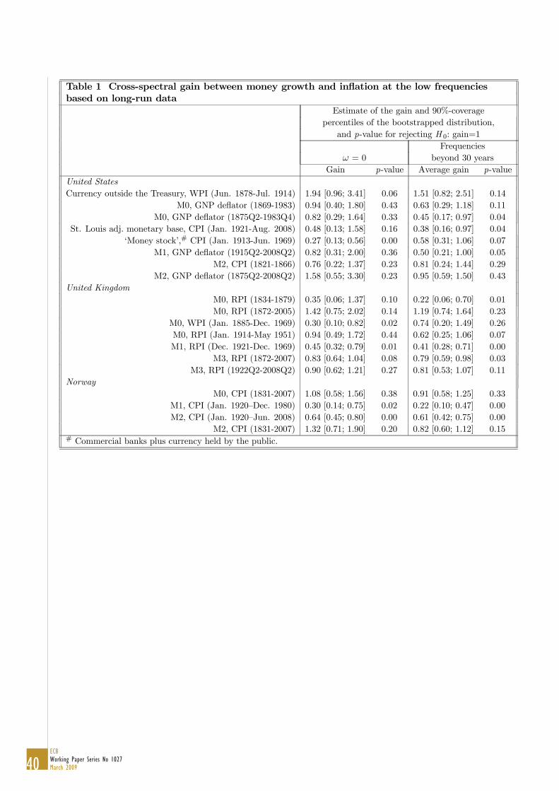
Table 1 Cross-spectral gain between money growth and inflation at the low frequenciesbased on long-run data

Estimate of the gain and 90%-coveragepercentiles of the bootstrapped distribution,

and p-value for rejecting H 0: gain=1Frequencies

ω = 0 beyond 30 yearsGain p-value Average gain p-value

United StatesCurrency outside the Treasury, WPI (Jun. 1878-Jul. 1914) 1.94 [0.96; 3.41] 0.06 1.51 [0.82; 2.51] 0.14

M0, GNP deflator (1869-1983) 0.94 [0.40; 1.80] 0.43 0.63 [0.29; 1.18] 0.11M0, GNP deflator (1875Q2-1983Q4) 0.82 [0.29; 1.64] 0.33 0.45 [0.17; 0.97] 0.04

St. Louis adj. monetary base, CPI (Jan. 1921-Aug. 2008) 0.48 [0.13; 1.58] 0.16 0.38 [0.16; 0.97] 0.04‘Money stock’,# CPI (Jan. 1913-Jun. 1969) 0.27 [0.13; 0.56] 0.00 0.58 [0.31; 1.06] 0.07

M1, GNP deflator (1915Q2-2008Q2) 0.82 [0.31; 2.00] 0.36 0.50 [0.21; 1.00] 0.05M2, CPI (1821-1866) 0.76 [0.22; 1.37] 0.23 0.81 [0.24; 1.44] 0.29

M2, GNP deflator (1875Q2-2008Q2) 1.58 [0.55; 3.30] 0.23 0.95 [0.59; 1.50] 0.43United Kingdom

M0, RPI (1834-1879) 0.35 [0.06; 1.37] 0.10 0.22 [0.06; 0.70] 0.01M0, RPI (1872-2005) 1.42 [0.75; 2.02] 0.14 1.19 [0.74; 1.64] 0.23

M0, WPI (Jan. 1885-Dec. 1969) 0.30 [0.10; 0.82] 0.02 0.74 [0.20; 1.49] 0.26M0, RPI (Jan. 1914-May 1951) 0.94 [0.49; 1.72] 0.44 0.62 [0.25; 1.06] 0.07M1, RPI (Dec. 1921-Dec. 1969) 0.45 [0.32; 0.79] 0.01 0.41 [0.28; 0.71] 0.00

M3, RPI (1872-2007) 0.83 [0.64; 1.04] 0.08 0.79 [0.59; 0.98] 0.03M3, RPI (1922Q2-2008Q2) 0.90 [0.62; 1.21] 0.27 0.81 [0.53; 1.07] 0.11

NorwayM0, CPI (1831-2007) 1.08 [0.58; 1.56] 0.38 0.91 [0.58; 1.25] 0.33

M1, CPI (Jan. 1920—Dec. 1980) 0.30 [0.14; 0.75] 0.02 0.22 [0.10; 0.47] 0.00M2, CPI (Jan. 1920—Jun. 2008) 0.64 [0.45; 0.80] 0.00 0.61 [0.42; 0.75] 0.00

M2, CPI (1831-2007) 1.32 [0.71; 1.90] 0.20 0.82 [0.60; 1.12] 0.15# Commercial banks plus currency held by the public.


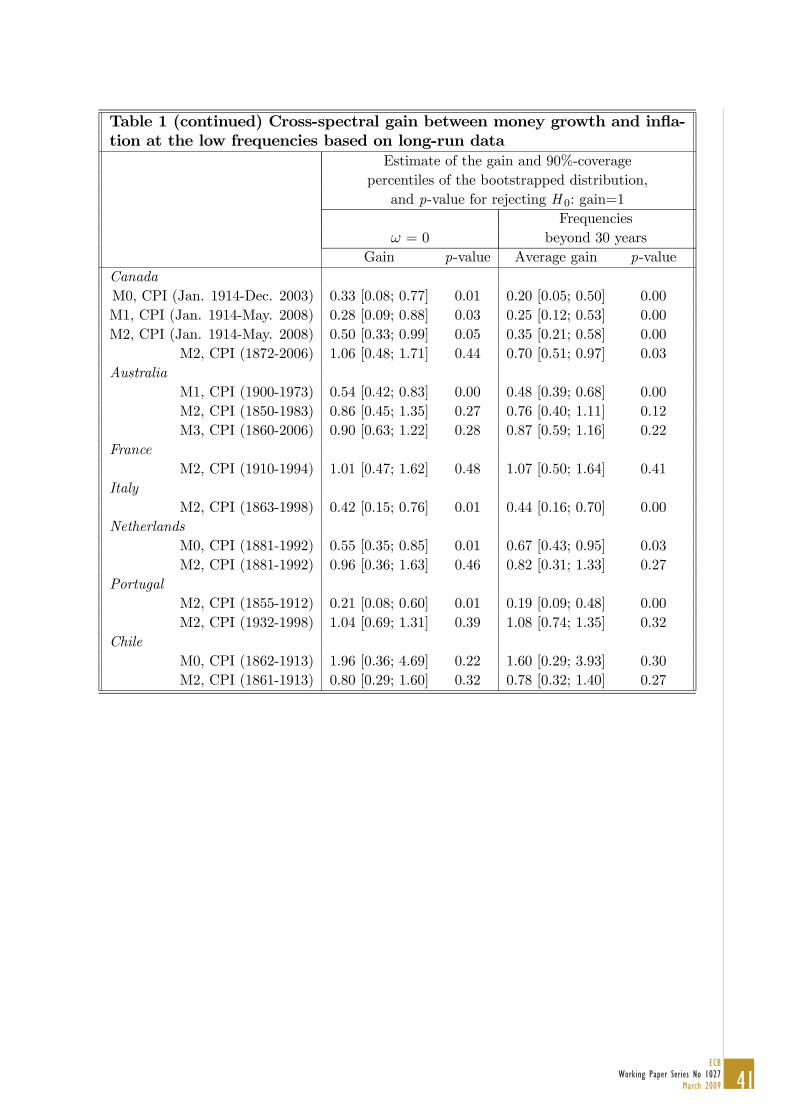
Table 1 (continued) Cross-spectral gain between money growth and infla-tion at the low frequencies based on long-run data




CanadaM0, CPI (Jan. 1914-Dec. 2003) 0.33 [0.08; 0.77] 0.01 0.20 [0.05; 0.50] 0.00M1, CPI (Jan. 1914-May. 2008) 0.28 [0.09; 0.88] 0.03 0.25 [0.12; 0.53] 0.00M2, CPI (Jan. 1914-May. 2008) 0.50 [0.33; 0.99] 0.05 0.35 [0.21; 0.58] 0.00

M2, CPI (1872-2006) 1.06 [0.48; 1.71] 0.44 0.70 [0.51; 0.97] 0.03Australia

M1, CPI (1900-1973) 0.54 [0.42; 0.83] 0.00 0.48 [0.39; 0.68] 0.00M2, CPI (1850-1983) 0.86 [0.45; 1.35] 0.27 0.76 [0.40; 1.11] 0.12M3, CPI (1860-2006) 0.90 [0.63; 1.22] 0.28 0.87 [0.59; 1.16] 0.22

FranceM2, CPI (1910-1994) 1.01 [0.47; 1.62] 0.48 1.07 [0.50; 1.64] 0.41

ItalyM2, CPI (1863-1998) 0.42 [0.15; 0.76] 0.01 0.44 [0.16; 0.70] 0.00

NetherlandsM0, CPI (1881-1992) 0.55 [0.35; 0.85] 0.01 0.67 [0.43; 0.95] 0.03M2, CPI (1881-1992) 0.96 [0.36; 1.63] 0.46 0.82 [0.31; 1.33] 0.27

PortugalM2, CPI (1855-1912) 0.21 [0.08; 0.60] 0.01 0.19 [0.09; 0.48] 0.00M2, CPI (1932-1998) 1.04 [0.69; 1.31] 0.39 1.08 [0.74; 1.35] 0.32

ChileM0, CPI (1862-1913) 1.96 [0.36; 4.69] 0.22 1.60 [0.29; 3.93] 0.30M2, CPI (1861-1913) 0.80 [0.29; 1.60] 0.32 0.78 [0.32; 1.40] 0.27

41ECB


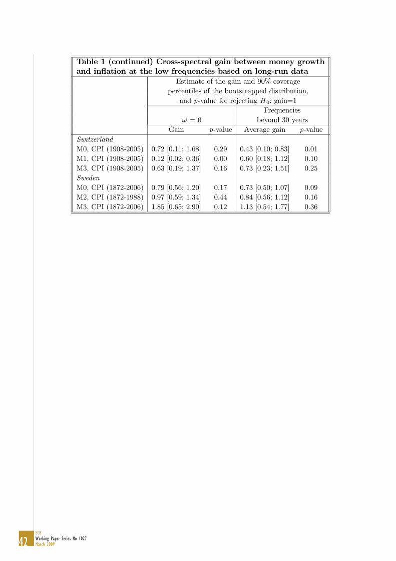
Table 1 (continued) Cross-spectral gain between money growthand inflation at the low frequencies based on long-run data




SwitzerlandM0, CPI (1908-2005) 0.72 [0.11; 1.68] 0.29 0.43 [0.10; 0.83] 0.01M1, CPI (1908-2005) 0.12 [0.02; 0.36] 0.00 0.60 [0.18; 1.12] 0.10M3, CPI (1908-2005) 0.63 [0.19; 1.37] 0.16 0.73 [0.23; 1.51] 0.25SwedenM0, CPI (1872-2006) 0.79 [0.56; 1.20] 0.17 0.73 [0.50; 1.07] 0.09M2, CPI (1872-1988) 0.97 [0.59; 1.34] 0.44 0.84 [0.56; 1.12] 0.16M3, CPI (1872-2006) 1.85 [0.65; 2.90] 0.12 1.13 [0.54; 1.77] 0.36


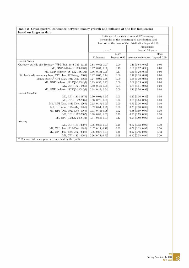
Table 2 Cross-spectral coherence between money growth and inflation at the low frequenciesbased on long-run data

Estimate of the coherence and 90%-coveragepercentiles of the bootstrapped distribution, andfraction of the mass of the distribution beyond 0.99

Frequenciesω = 0 beyond 30 years

Mass MassCoherence beyond 0.99 Average coherence beyond 0.99

United StatesCurrency outside the Treasury, WPI (Jun. 1878-Jul. 1914) 0.88 [0.66; 0.97] 0.00 0.85 [0.65; 0.96] 0.00

M0, GNP deflator (1869-1983) 0.97 [0.87; 1.00] 0.19 0.61 [0.27; 0.90] 0.00M0, GNP deflator (1875Q2-1983Q4) 0.96 [0.83; 0.99] 0.11 0.50 [0.20; 0.87] 0.00

St. Louis adj. monetary base, CPI (Jan. 1921-Aug. 2008) 0.22 [0.05; 0.74] 0.00 0.46 [0.18; 0.84] 0.00‘Money stock’,# CPI (Jan. 1913-Jun. 1969) 0.27 [0.07; 0.78] 0.00 0.75 [0.39; 0.95] 0.00

M1, GNP deflator (1915Q2-2008Q2) 0.63 [0.33; 0.93] 0.00 0.68 [0.33; 0.94] 0.00M2, CPI (1821-1866) 0.92 [0.47; 0.99] 0.04 0.84 [0.31; 0.97] 0.00

M2, GNP deflator (1875Q2-2008Q2) 0.68 [0.27; 0.94] 0.00 0.80 [0.56; 0.93] 0.00United Kingdom

M0, RPI (1834-1879) 0.50 [0.08; 0.94] 0.01 0.47 [0.16; 0.85] 0.00M0, RPI (1872-2005) 0.98 [0.78; 1.00] 0.25 0.89 [0.64; 0.97] 0.00

M0, WPI (Jan. 1885-Dec. 1969) 0.52 [0.17; 0.91] 0.00 0.75 [0.26; 0.95] 0.00M0, RPI (Jan. 1914-May 1951) 0.82 [0.54; 0.96] 0.00 0.70 [0.30; 0.89] 0.00M1, RPI (Dec. 1921-Dec. 1969) 0.93 [0.75; 0.98] 0.02 0.88 [0.69; 0.97] 0.00

M3, RPI (1872-2007) 0.98 [0.89; 1.00] 0.29 0.93 [0.79; 0.98] 0.00M3, RPI (1922Q2-2008Q2) 0.97 [0.85; 1.00] 0.17 0.95 [0.80; 0.99] 0.02

NorwayM0, CPI (1831-2007) 0.98 [0.81; 1.00] 0.26 0.87 [0.63; 0.96] 0.00

M1, CPI (Jan. 1920—Dec. 1980) 0.47 [0.14; 0.89] 0.00 0.71 [0.33; 0.95] 0.00M2, CPI (Jan. 1920—Jun. 2008) 0.98 [0.87; 1.00] 0.31 0.97 [0.86; 0.99] 0.13

M2, CPI (1831-2007) 0.96 [0.74; 0.99] 0.08 0.90 [0.75; 0.97] 0.00# Commercial banks plus currency held by the public.

43ECB


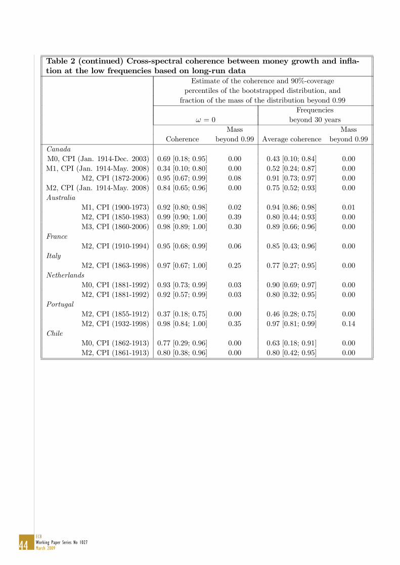
Table 2 (continued) Cross-spectral coherence between money growth and infla-tion at the low frequencies based on long-run data




CanadaM0, CPI (Jan. 1914-Dec. 2003) 0.69 [0.18; 0.95] 0.00 0.43 [0.10; 0.84] 0.00M1, CPI (Jan. 1914-May. 2008) 0.34 [0.10; 0.80] 0.00 0.52 [0.24; 0.87] 0.00

M2, CPI (1872-2006) 0.95 [0.67; 0.99] 0.08 0.91 [0.73; 0.97] 0.00M2, CPI (Jan. 1914-May. 2008) 0.84 [0.65; 0.96] 0.00 0.75 [0.52; 0.93] 0.00Australia

M1, CPI (1900-1973) 0.92 [0.80; 0.98] 0.02 0.94 [0.86; 0.98] 0.01M2, CPI (1850-1983) 0.99 [0.90; 1.00] 0.39 0.80 [0.44; 0.93] 0.00M3, CPI (1860-2006) 0.98 [0.89; 1.00] 0.30 0.89 [0.66; 0.96] 0.00

FranceM2, CPI (1910-1994) 0.95 [0.68; 0.99] 0.06 0.85 [0.43; 0.96] 0.00

ItalyM2, CPI (1863-1998) 0.97 [0.67; 1.00] 0.25 0.77 [0.27; 0.95] 0.00

NetherlandsM0, CPI (1881-1992) 0.93 [0.73; 0.99] 0.03 0.90 [0.69; 0.97] 0.00M2, CPI (1881-1992) 0.92 [0.57; 0.99] 0.03 0.80 [0.32; 0.95] 0.00

PortugalM2, CPI (1855-1912) 0.37 [0.18; 0.75] 0.00 0.46 [0.28; 0.75] 0.00M2, CPI (1932-1998) 0.98 [0.84; 1.00] 0.35 0.97 [0.81; 0.99] 0.14

ChileM0, CPI (1862-1913) 0.77 [0.29; 0.96] 0.00 0.63 [0.18; 0.91] 0.00M2, CPI (1861-1913) 0.80 [0.38; 0.96] 0.00 0.80 [0.42; 0.95] 0.00


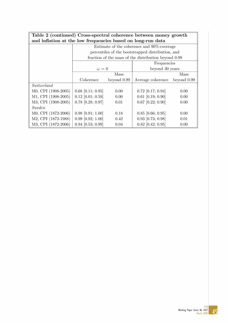
Table 2 (continued) Cross-spectral coherence between money growthand inflation at the low frequencies based on long-run data




SwitzerlandM0, CPI (1908-2005) 0.68 [0.11; 0.95] 0.00 0.72 [0.17; 0.94] 0.00M1, CPI (1908-2005) 0.12 [0.01; 0.59] 0.00 0.61 [0.19; 0.90] 0.00M3, CPI (1908-2005) 0.78 [0.28; 0.97] 0.01 0.67 [0.22; 0.90] 0.00SwedenM0, CPI (1872-2006) 0.98 [0.91; 1.00] 0.18 0.85 [0.66; 0.95] 0.00M2, CPI (1872-1988) 0.99 [0.92; 1.00] 0.42 0.93 [0.73; 0.98] 0.01M3, CPI (1872-2006) 0.94 [0.53; 0.99] 0.04 0.82 [0.42; 0.95] 0.00

45ECB


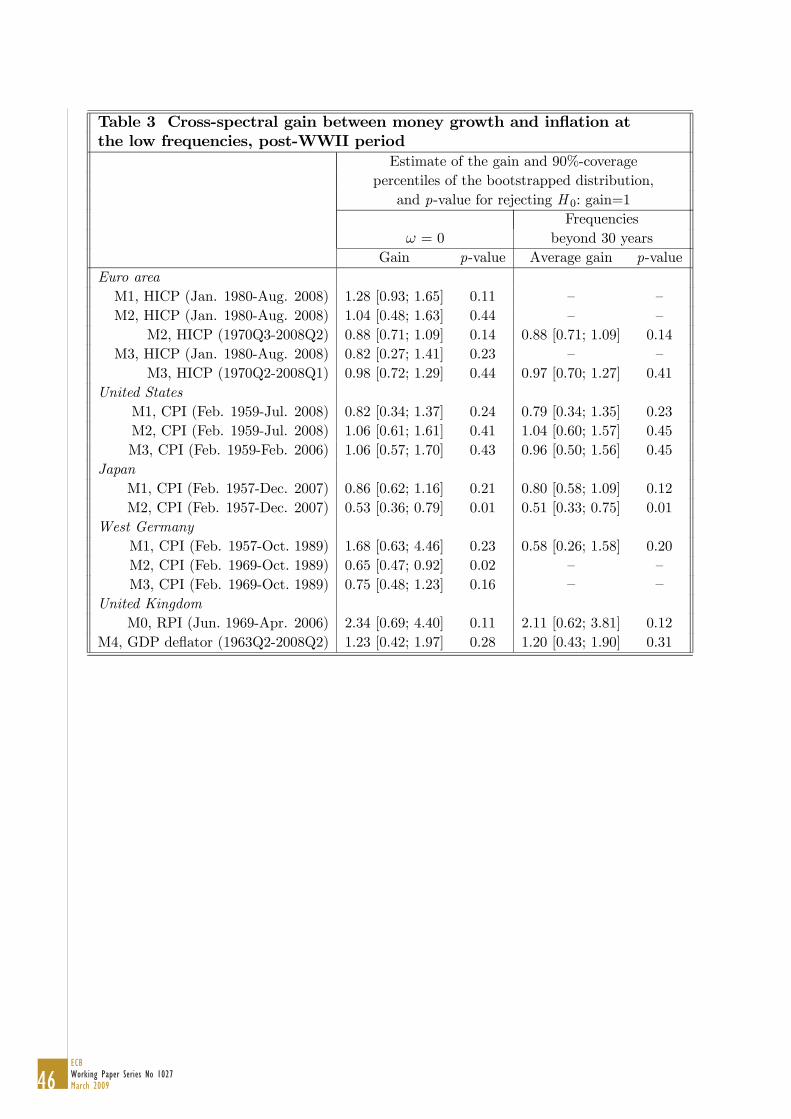
Table 3 Cross-spectral gain between money growth and inflation atthe low frequencies, post-WWII period




Euro areaM1, HICP (Jan. 1980-Aug. 2008) 1.28 [0.93; 1.65] 0.11 — —M2, HICP (Jan. 1980-Aug. 2008) 1.04 [0.48; 1.63] 0.44 — —

M2, HICP (1970Q3-2008Q2) 0.88 [0.71; 1.09] 0.14 0.88 [0.71; 1.09] 0.14M3, HICP (Jan. 1980-Aug. 2008) 0.82 [0.27; 1.41] 0.23 — —

M3, HICP (1970Q2-2008Q1) 0.98 [0.72; 1.29] 0.44 0.97 [0.70; 1.27] 0.41United States

M1, CPI (Feb. 1959-Jul. 2008) 0.82 [0.34; 1.37] 0.24 0.79 [0.34; 1.35] 0.23M2, CPI (Feb. 1959-Jul. 2008) 1.06 [0.61; 1.61] 0.41 1.04 [0.60; 1.57] 0.45M3, CPI (Feb. 1959-Feb. 2006) 1.06 [0.57; 1.70] 0.43 0.96 [0.50; 1.56] 0.45

JapanM1, CPI (Feb. 1957-Dec. 2007) 0.86 [0.62; 1.16] 0.21 0.80 [0.58; 1.09] 0.12M2, CPI (Feb. 1957-Dec. 2007) 0.53 [0.36; 0.79] 0.01 0.51 [0.33; 0.75] 0.01

West GermanyM1, CPI (Feb. 1957-Oct. 1989) 1.68 [0.63; 4.46] 0.23 0.58 [0.26; 1.58] 0.20M2, CPI (Feb. 1969-Oct. 1989) 0.65 [0.47; 0.92] 0.02 — —M3, CPI (Feb. 1969-Oct. 1989) 0.75 [0.48; 1.23] 0.16 — —

United KingdomM0, RPI (Jun. 1969-Apr. 2006) 2.34 [0.69; 4.40] 0.11 2.11 [0.62; 3.81] 0.12

M4, GDP deflator (1963Q2-2008Q2) 1.23 [0.42; 1.97] 0.28 1.20 [0.43; 1.90] 0.31


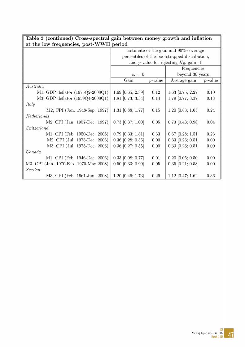
Table 3 (continued) Cross-spectral gain between money growth and inflationat the low frequencies, post-WWII period




AustraliaM1, GDP deflator (1975Q2-2008Q1) 1.69 [0.65; 2.39] 0.12 1.63 [0.75; 2.27] 0.10M3, GDP deflator (1959Q4-2008Q1) 1.81 [0.73; 3.34] 0.14 1.79 [0.77; 3.37] 0.13

ItalyM2, CPI (Jan. 1948-Sep. 1997) 1.31 [0.88; 1.77] 0.15 1.20 [0.83; 1.65] 0.24

NetherlandsM2, CPI (Jan. 1957-Dec. 1997) 0.73 [0.37; 1.00] 0.05 0.73 [0.43; 0.98] 0.04

SwitzerlandM1, CPI (Feb. 1950-Dec. 2006) 0.79 [0.33; 1.81] 0.33 0.67 [0.28; 1.51] 0.23M2, CPI (Jul. 1975-Dec. 2006) 0.36 [0.28; 0.55] 0.00 0.33 [0.26; 0.51] 0.00M3, CPI (Jul. 1975-Dec. 2006) 0.36 [0.27; 0.55] 0.00 0.33 [0.26; 0.51] 0.00

CanadaM1, CPI (Feb. 1946-Dec. 2006) 0.33 [0.08; 0.77] 0.01 0.20 [0.05; 0.50] 0.00

M3, CPI (Jan. 1970-Feb. 1970-May 2008) 0.50 [0.33; 0.99] 0.05 0.35 [0.21; 0.58] 0.00Sweden

M3, CPI (Feb. 1961-Jun. 2008) 1.20 [0.46; 1.73] 0.29 1.12 [0.47; 1.62] 0.36

47ECB


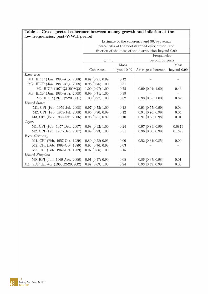
Table 4 Cross-spectral coherence between money growth and inflation at thelow frequencies, post-WWII period




Euro areaM1, HICP (Jan. 1980-Aug. 2008) 0.97 [0.91; 0.99] 0.12 — —M2, HICP (Jan. 1980-Aug. 2008) 0.98 [0.76; 1.00] 0.31 — —

M2, HICP (1970Q3-2008Q2) 1.00 [0.97; 1.00] 0.75 0.99 [0.94; 1.00] 0.43M3, HICP (Jan. 1980-Aug. 2008) 0.99 [0.71; 1.00] 0.39 — —

M3, HICP (1970Q2-2008Q1) 1.00 [0.97; 1.00] 0.82 0.98 [0.88; 1.00] 0.32United States

M1, CPI (Feb. 1959-Jul. 2008) 0.97 [0.73; 1.00] 0.18 0.91 [0.57; 0.99] 0.03M2, CPI (Feb. 1959-Jul. 2008) 0.96 [0.90; 0.99] 0.12 0.94 [0.76; 0.99] 0.04M3, CPI (Feb. 1959-Feb. 2006) 0.96 [0.81; 0.99] 0.10 0.91 [0.68; 0.98] 0.01

JapanM1, CPI (Feb. 1957-Dec. 2007) 0.98 [0.92; 1.00] 0.24 0.97 [0.89; 0.99] 0.0879M2, CPI (Feb. 1957-Dec. 2007) 0.99 [0.93; 1.00] 0.51 0.96 [0.80; 0.99] 0.1395

West GermanyM1, CPI (Feb. 1957-Oct. 1989) 0.80 [0.58; 0.96] 0.00 0.52 [0.31; 0.85] 0.00M2, CPI (Feb. 1969-Oct. 1989) 0.93 [0.76; 0.99] 0.03 — —M3, CPI (Feb. 1969-Oct. 1989) 0.97 [0.86; 1.00] 0.15 — —

United KingdomM0, RPI (Jun. 1969-Apr. 2006) 0.91 [0.47; 0.99] 0.05 0.86 [0.37; 0.98] 0.01

M4, GDP deflator (1963Q2-2008Q2) 0.97 [0.69; 1.00] 0.24 0.93 [0.49; 0.99] 0.06


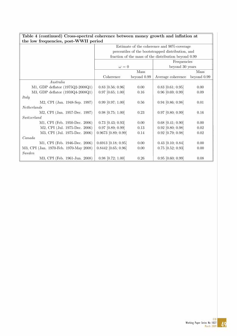
Table 4 (continued) Cross-spectral coherence between money growth and inflation atthe low frequencies, post-WWII period




AustraliaM1, GDP deflator (1975Q2-2008Q1) 0.83 [0.56; 0.96] 0.00 0.83 [0.61; 0.95] 0.00M3, GDP deflator (1959Q4-2008Q1) 0.97 [0.65; 1.00] 0.16 0.96 [0.69; 0.99] 0.09

ItalyM2, CPI (Jan. 1948-Sep. 1997) 0.99 [0.97; 1.00] 0.56 0.94 [0.86; 0.98] 0.01

NetherlandsM2, CPI (Jan. 1957-Dec. 1997) 0.98 [0.75; 1.00] 0.23 0.97 [0.80; 0.99] 0.16

SwitzerlandM1, CPI (Feb. 1950-Dec. 2006) 0.73 [0.43; 0.93] 0.00 0.68 [0.41; 0.90] 0.00M2, CPI (Jul. 1975-Dec. 2006) 0.97 [0.89; 0.99] 0.13 0.92 [0.80; 0.98] 0.02M3, CPI (Jul. 1975-Dec. 2006) 0.9673 [0.89; 0.99] 0.14 0.92 [0.79; 0.98] 0.02

CanadaM1, CPI (Feb. 1946-Dec. 2006) 0.6913 [0.18; 0.95] 0.00 0.43 [0.10; 0.84] 0.00

M3, CPI (Jan. 1970-Feb. 1970-May 2008) 0.8442 [0.65; 0.96] 0.00 0.75 [0.52; 0.93] 0.00Sweden

M3, CPI (Feb. 1961-Jun. 2008) 0.98 [0.72; 1.00] 0.26 0.95 [0.60; 0.99] 0.08

49ECB


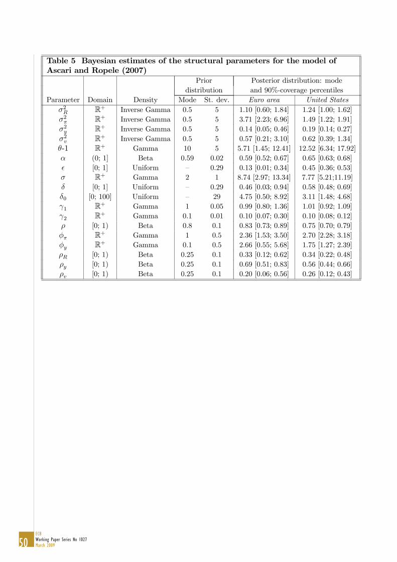
Table 5 Bayesian estimates of the structural parameters for the model ofAscari and Ropele (2007)

Prior Posterior distribution: modedistribution and 90%-coverage percentiles

Parameter Domain Density Mode St. dev. Euro area United Statesσ2R R+ Inverse Gamma 0.5 5 1.10 [0.60; 1.84] 1.24 [1.00; 1.62]σ2π R+ Inverse Gamma 0.5 5 3.71 [2.23; 6.96] 1.49 [1.22; 1.91]σ2y R+ Inverse Gamma 0.5 5 0.14 [0.05; 0.46] 0.19 [0.14; 0.27]σ2v R+ Inverse Gamma 0.5 5 0.57 [0.21; 3.10] 0.62 [0.39; 1.34]θ-1 R+ Gamma 10 5 5.71 [1.45; 12.41] 12.52 [6.34; 17.92]α (0; 1] Beta 0.59 0.02 0.59 [0.52; 0.67] 0.65 [0.63; 0.68]

[0; 1] Uniform — 0.29 0.13 [0.01; 0.34] 0.45 [0.36; 0.53]σ R+ Gamma 2 1 8.74 [2.97; 13.34] 7.77 [5.21;11.19]δ [0; 1] Uniform — 0.29 0.46 [0.03; 0.94] 0.58 [0.48; 0.69]δ0 [0; 100] Uniform — 29 4.75 [0.50; 8.92] 3.11 [1.48; 4.68]γ1 R+ Gamma 1 0.05 0.99 [0.80; 1.36] 1.01 [0.92; 1.09]γ2 R+ Gamma 0.1 0.01 0.10 [0.07; 0.30] 0.10 [0.08; 0.12]ρ [0; 1) Beta 0.8 0.1 0.83 [0.73; 0.89] 0.75 [0.70; 0.79]φπ R+ Gamma 1 0.5 2.36 [1.53; 3.50] 2.70 [2.28; 3.18]φy R+ Gamma 0.1 0.5 2.66 [0.55; 5.68] 1.75 [1.27; 2.39]ρR [0; 1) Beta 0.25 0.1 0.33 [0.12; 0.62] 0.34 [0.22; 0.48]ρy [0; 1) Beta 0.25 0.1 0.69 [0.51; 0.83] 0.56 [0.44; 0.66]ρv [0; 1) Beta 0.25 0.1 0.20 [0.06; 0.56] 0.26 [0.12; 0.43]


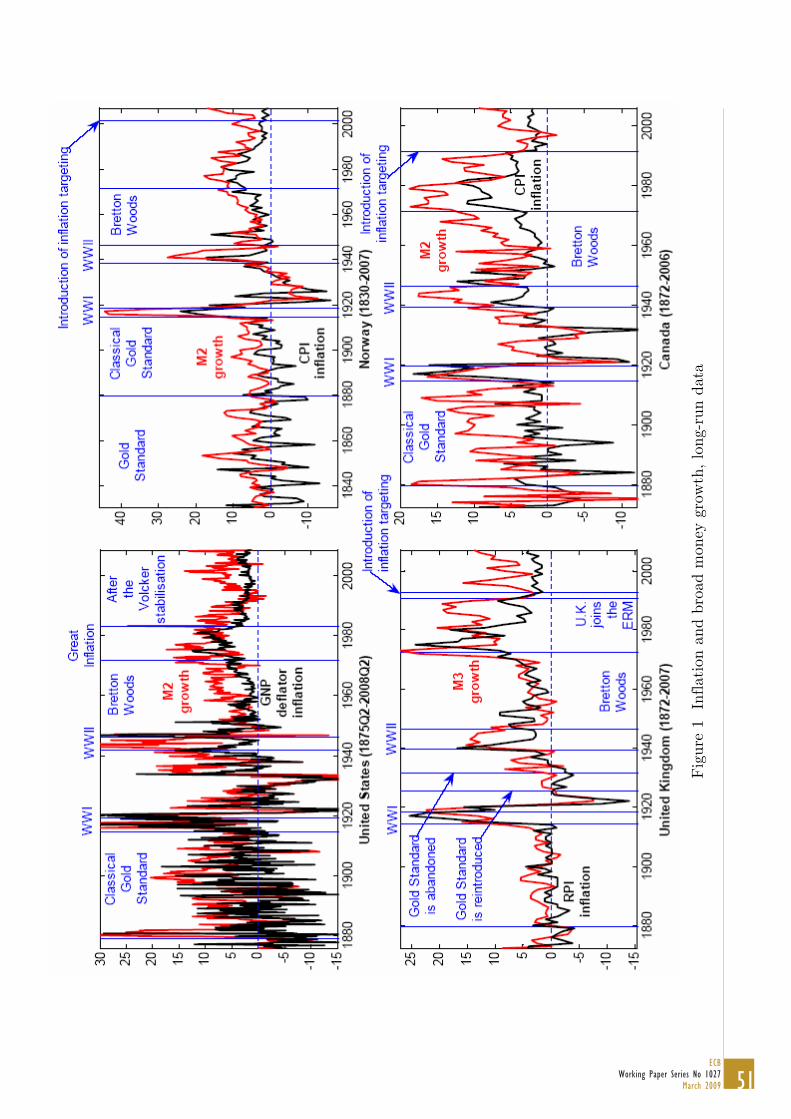
Fig

ure

1 I

nfla

tion

and

bro

ad m

oney

gro

wth

, lo

ng-r

un d

ata

51ECB


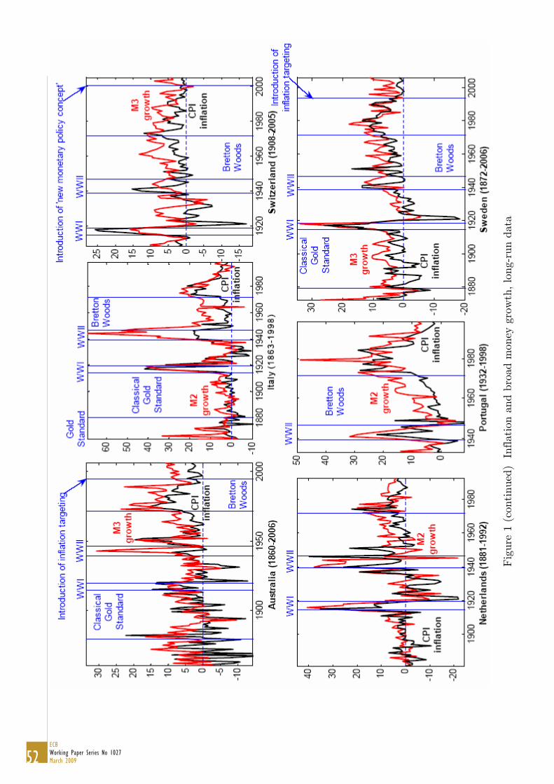
Fig

ure

1 (c

onti

nued

) I

nfla

tion

an d

bro

ad m

oney

gro

wth

, lo

ng-r

un d

ata


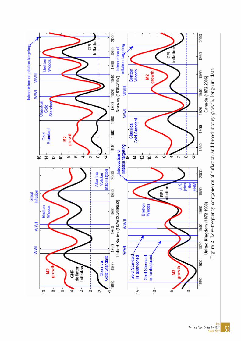
Fig

ure

2 L

ow-fre

quen

cy c

ompo

n ent

s of

inf

lati

on a

nd b

road

mon

ey g

row

th, lo

ng-r

un d

ata

53ECB


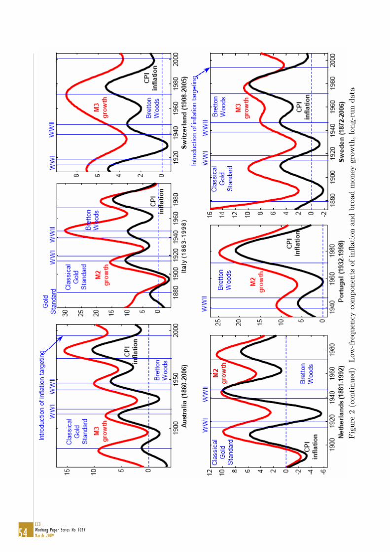
Fig

ure

2 (c

onti

nued

) L

ow-fre

quen

cy c

ompo

nent

s of

inf

lati

on a

nd b

road

mon

ey g

row

th, lo

ng-r

un d

ata


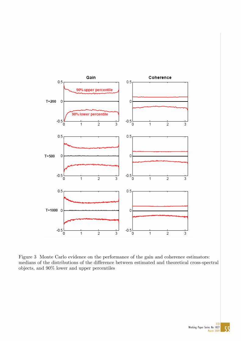
Figure 3 Monte Carlo evidence on the performance of the gain and coherence estimators: medians of the distributions of the difference between estimated and theoretical cross-spectral objects, and 90% lower and upper percentiles

55

ECBWorking Paper Series No 1027

March 2009

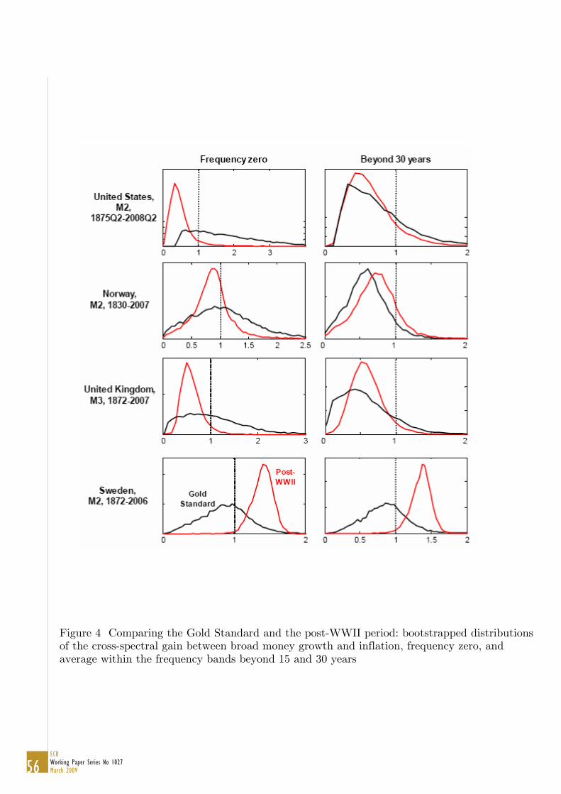
Figure 4 Comparing the Gold Standard and the post-WWII period: bootstrapped distributions of the cross-spectral gain between broad money growth and inflation, frequency zero, and average within the frequency bands beyond 15 and 30 years

56

ECBWorking Paper Series No 1027March 2009

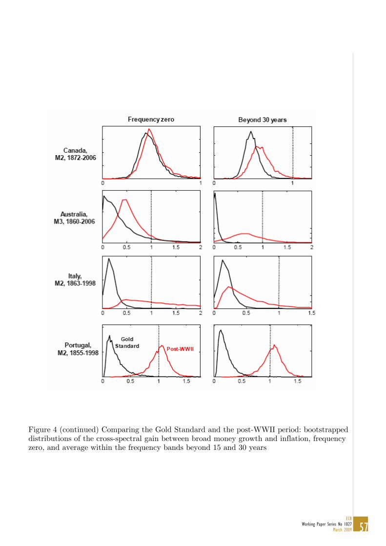
Figure 4 (continued) Comparing the Gold Standard and the post-WWII period: bootstrapped distributions of the cross-spectral gain between broad money growth and inflation, frequency zero, and average within the frequency bands beyond 15 and 30 years

57


March 2009

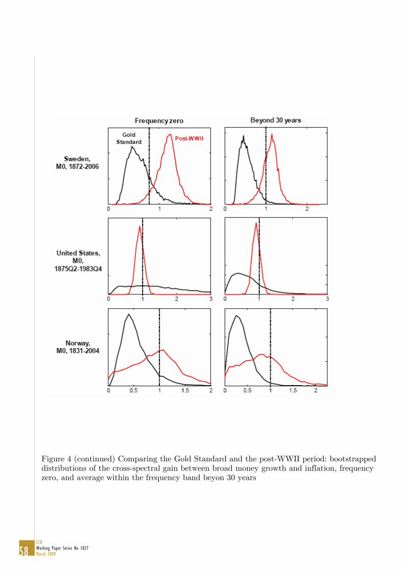
Figure 4 (continued) Comparing the Gold Standard and the post-WWII period: bootstrapped distributions of the cross-spectral gain between broad money growth and inflation, frequency zero, and average within the frequency band beyon 30 years

58


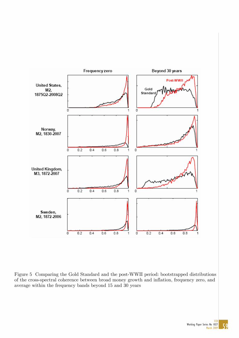
Figure 5 Comparing the Gold Standard and the post-WWII period: bootstrapped distributions of the cross-spectral coherence between broad money growth and inflation, frequency zero, and average within the frequency bands beyond 15 and 30 years

59


March 2009

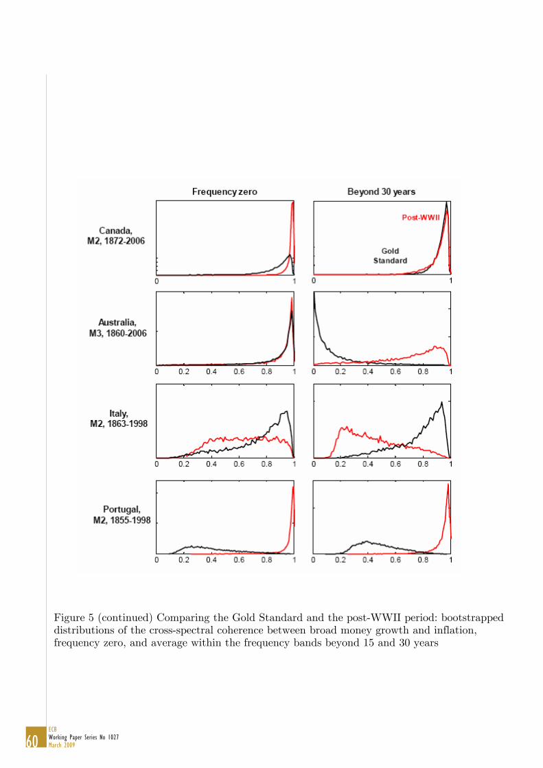
Figure 5 (continued) Comparing the Gold Standard and the post-WWII period: bootstrapped distributions of the cross-spectral coherence between broad money growth and inflation, frequency zero, and average within the frequency bands beyond 15 and 30 years

60


.

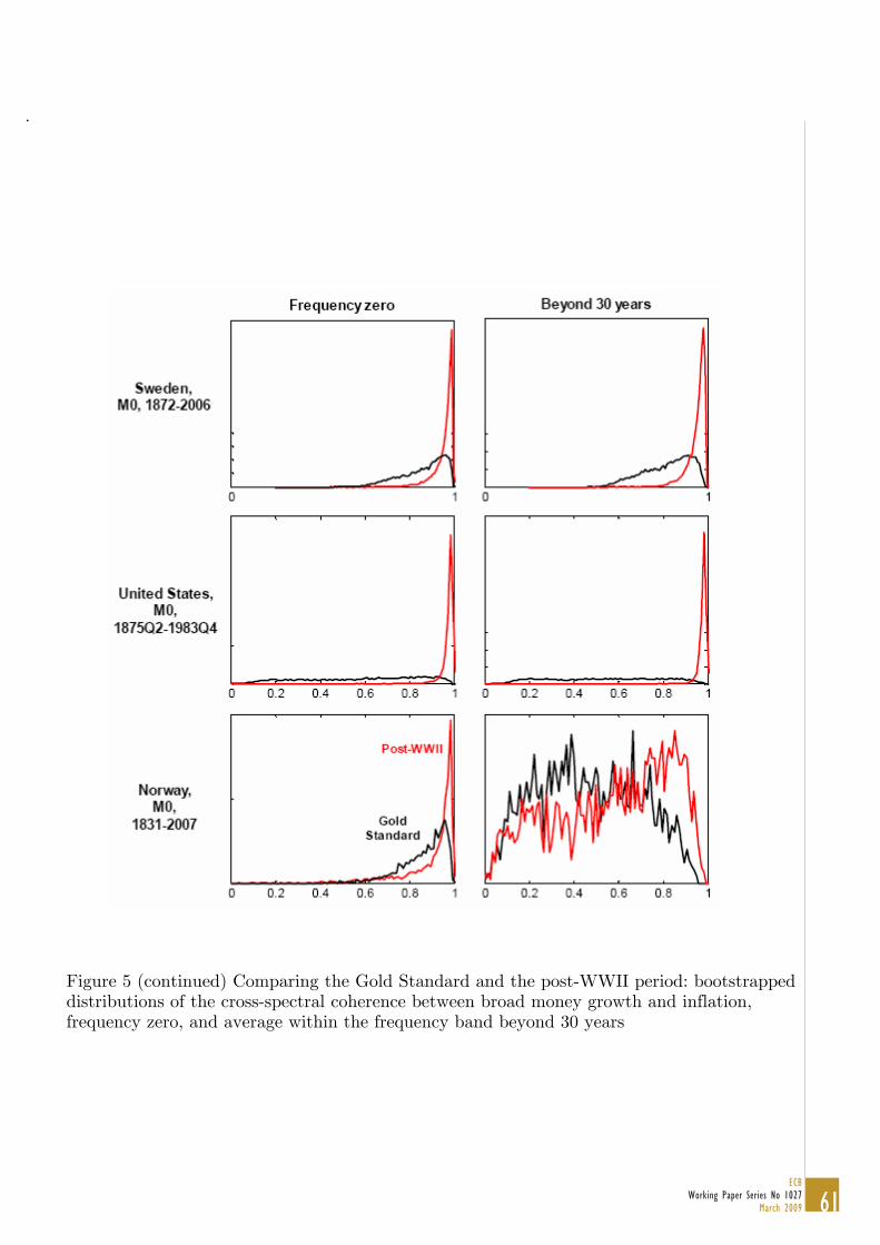
Figure 5 (continued) Comparing the Gold Standard and the post-WWII period: bootstrapped distributions of the cross-spectral coherence between broad money growth and inflation, frequency zero, and average within the frequency band beyond 30 years

61


March 2009

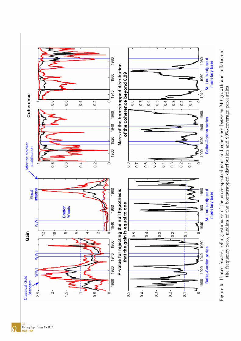
Fig

ure

6 U

nite

d St

ates

, ro

lling

est

imat

e s o

f th

e cr

oss-

spec

tral

gai

n an

d co

here

nce

betw

een

M0

grow

th a

nd inf

lati

on a

t

the

freq

uenc

y ze

ro, m

edia

n of

the

boo

tstr

appe

d di

stri

buti

on a

nd 9

0%-c

over

age

perc

enti

les


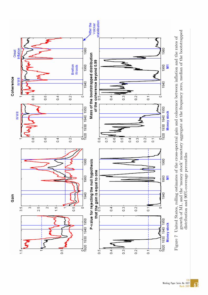
Fig

ure

7 U

nite

d St

ates

, ro

lling

est

imat

e s o

f th

e cr

oss-

spec

tral

gai

n an

d co

here

nce

betw

een

inflat

ion

and

the

rate

s of

grow

th o

f M

1, a

nd t

he ‘m

oney

sto

ck’ m

onet

ary

aggr

egat

e at

the

fre

quen

cy z

ero,

med

ian

of t

he b

oots

trap

ped

di

stri

buti

on a

nd 9

0%-c

over

age

perc

enti

les

63ECB


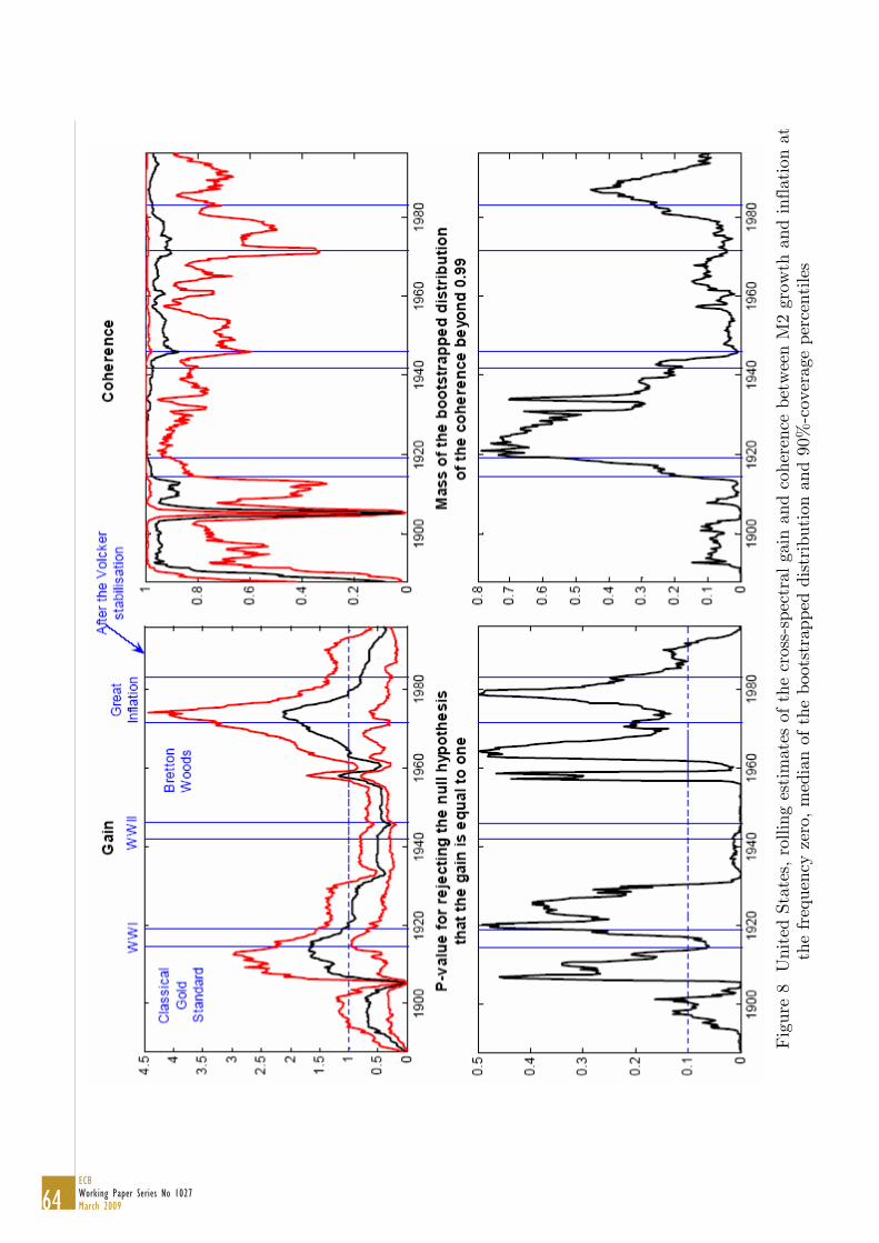
Fig

ure

8 U

nite

d St

ates

, ro

lling

est

imat

e s o

f th

e cr

oss-

spec

tral

gai

n an

d co

here

n ce

betw

een

M2

grow

th a

nd inf

lati

on a

t

the

freq

uenc

y ze

ro, m

edia

n of

the

boo

tstr

appe

d di

stri

buti

on a

nd 9

0%-c

over

age

perc

enti

les


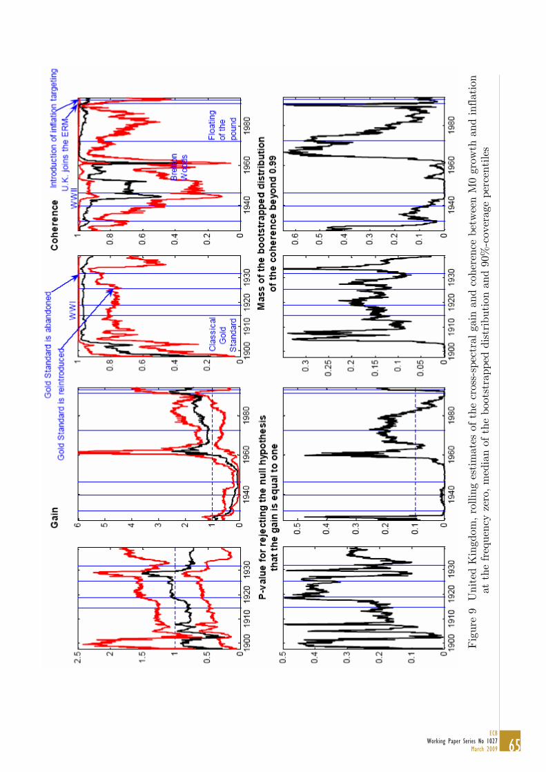
Fig

ure

9 U

nite

d K

ingd

om, ro

lling

est

imat

es o

f th

e cr

oss-

spec

tral

gai

n an

d co

here

nce

betw

een

M0

grow

th a

nd inf

lati

on

at

the

fre

quen

cy z

ero,

med

ian

of t

he b

oots

trap

ped

dist

ribu

tion

and

90%

-cov

erag

e pe

rcen

tile

s

65ECB


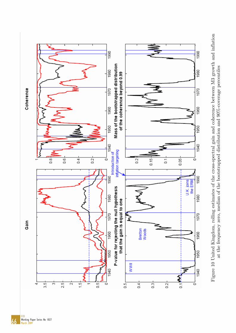
Fig

ure

10 U

nite

d K

ingd

om, ro

lling

est

imat

e s o

f th

e cr

oss-

spec

tral

gai

n an

d co

here

nce

betw

een

M3

grow

th a

nd inf

lati

on

at

the

fre

quen

cy z

ero,

med

ian

of t

he b

oots

trap

ped

dist

ribu

tion

and

90%

-cov

erag

e pe

rcen

tile

s


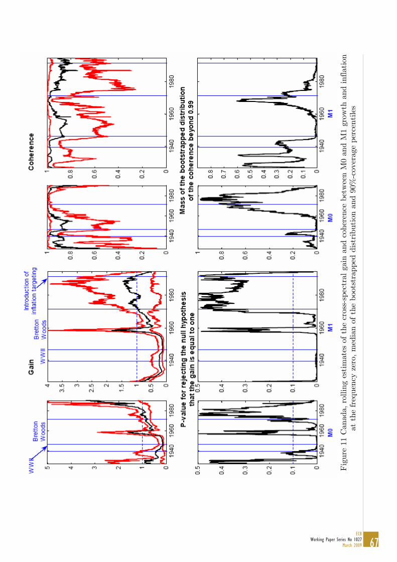
Fig

ure

11 C

anad

a, r

ollin

g es

tim

ates

of th

e cr

oss-

spec

tral

gai

n an

d co

here

nce

betw

een

M0

and

M1

grow

th a

nd inf

lati

on

at

the

fre

quen

cy z

ero,

med

ian

of t

he b

oots

trap

ped

dist

ribu

tion

and

90%

-cov

erag

e pe

rcen

tile

s

67ECB


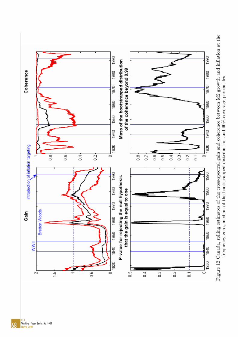
Fig

ure

12 C

anad

a, r

ollin

g es

tim

ates

of th

e cr

oss-

spec

tral

gai

n an

d co

here

nce

betw

een

M2

grow

th a

nd inf

lation

at

the

fr

eque

ncy

zero

, m

edia

n of

the

boo

tstr

appe

d di

stri

buti

on a

nd 9

0%-c

over

age

perc

enti

les


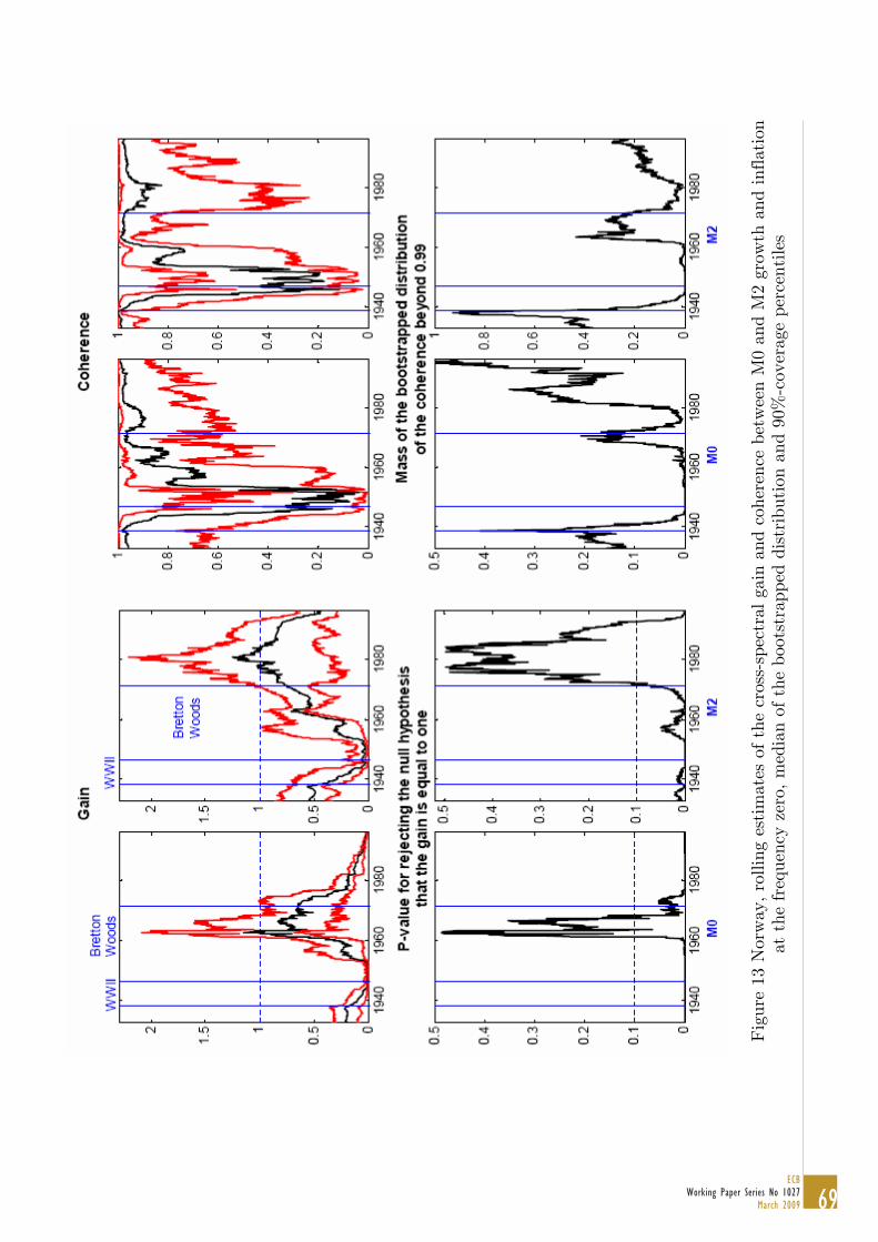
Fig

ure

13 N

orw

ay, ro

lling

est

imat

es o

f th

e cr

oss-

spec

tral

gai

n an

d co

here

nce

betw

een

M0

and

M2

grow

th a

nd inf

lati

on

at

the

fre

quen

cy z

ero,

med

ian

of t

he b

oots

trap

ped

dist

ribu

tion

and

90%

-cov

erag

e pe

rcen

tile

s

69ECB


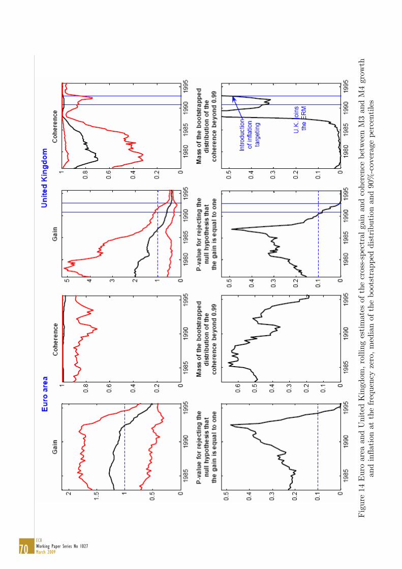
Fig

ure

14 E

uro

area

and

Uni

ted

Kin

gdom

, ro

llin g

est

imat

es o

f th

e cr

oss-

spec

tral

gai

n an

d co

here

nce

betw

een

M3

and

M4

grow

th

an

d in

flat

ion

at t

he fre

que n

cy z

ero,

med

ian

of t

he b

oots

trap

ped

dist

ribu

tion

and

90%

-cov

erag

e pe

rcen

tile

s


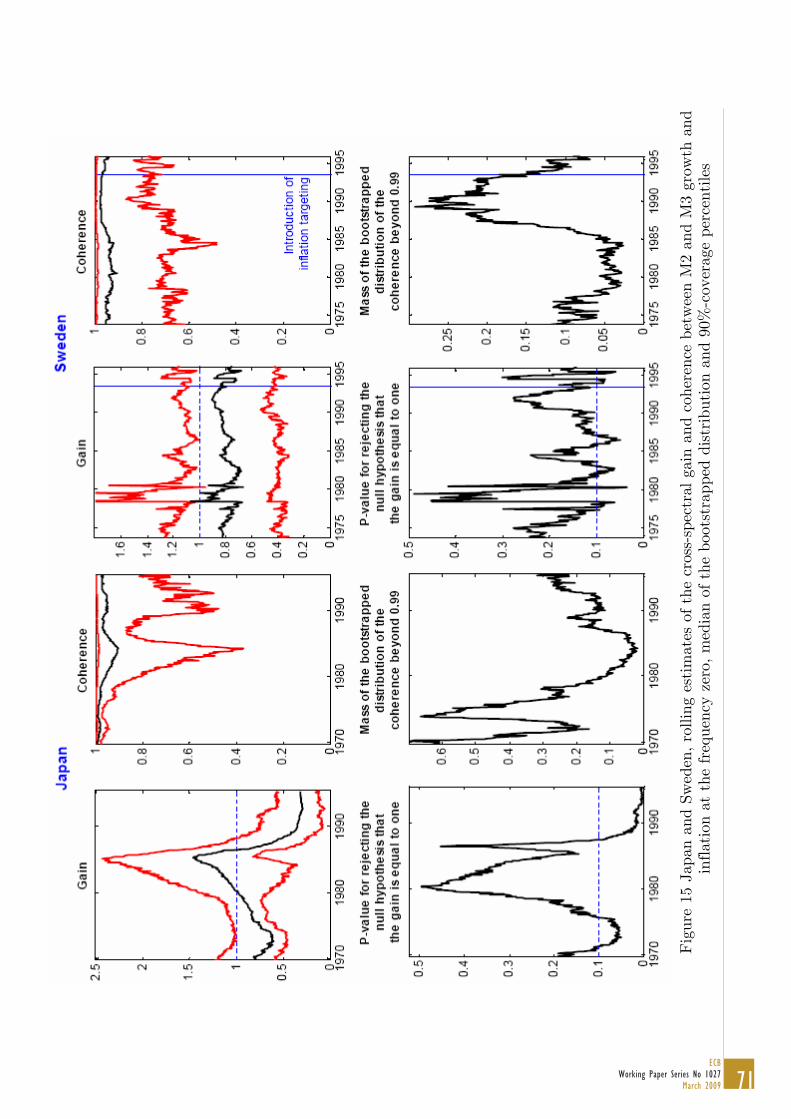
Fig

ure

15 J

apan

and

Sw

eden

, ro

lling

est

imat

es o

f th

e cr

oss-

spec

tral

gai

n an

d co

here

nce

betw

een

M2

and

M3

grow

th a

nd

in

flat

ion

at t

he fre

quen

cy z

ero,

med

ian

of t

he b

oots

trap

ped

dist

ribu

tion

and

90%

-cov

erag

e pe

rcen

tile

s

71ECB


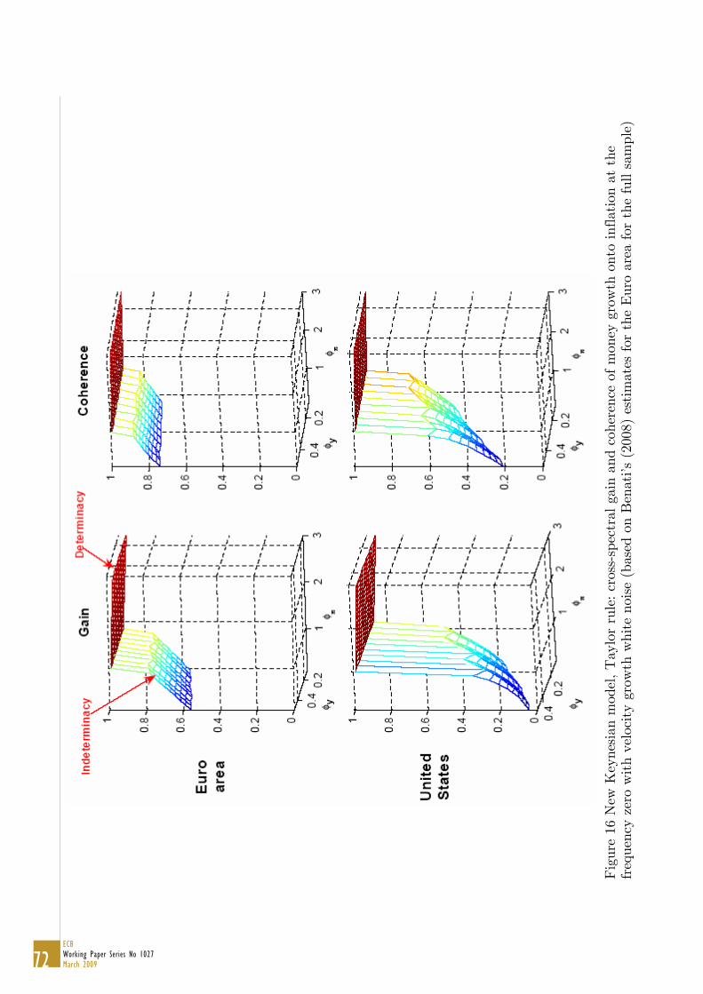
Fig

ure

16 N

ew K

eyne

sian

mod

el, T

aylo

r ru

le: cr

oss-

spec

tral

gai

n an

d co

here

nce

of m

oney

gro

wth

ont

o in

flat

ion

at t

he

freq

uenc

y ze

ro w

ith

velo

city

gro

wth

whi

t e n

oise

(ba

sed

on B

enat

i’s (

2008

) es

tim

ates

for

the

Eur

o ar

ea for

the

ful

l sa

mpl

e)


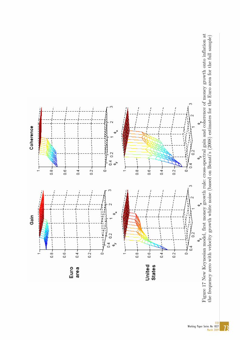
Fig

ure

17 N

ew K

eyne

sian

mod

el, firs

t m

oney

gro

wth

rul

e: c

ross

-spe

ctra

l ga

in a

nd c

oher

e nce

of m

oney

gro

wth

ont

o in

flat

ion

at

the

freq

uenc

y ze

ro w

ith

velo

city

gro

wth

whi

te n

oise

(ba

sed

on B

enat

i’s (

2008

) es

tim

ates

for

the

Eur

o ar

ea for

the

ful

l sa

mpl

e)

73ECB


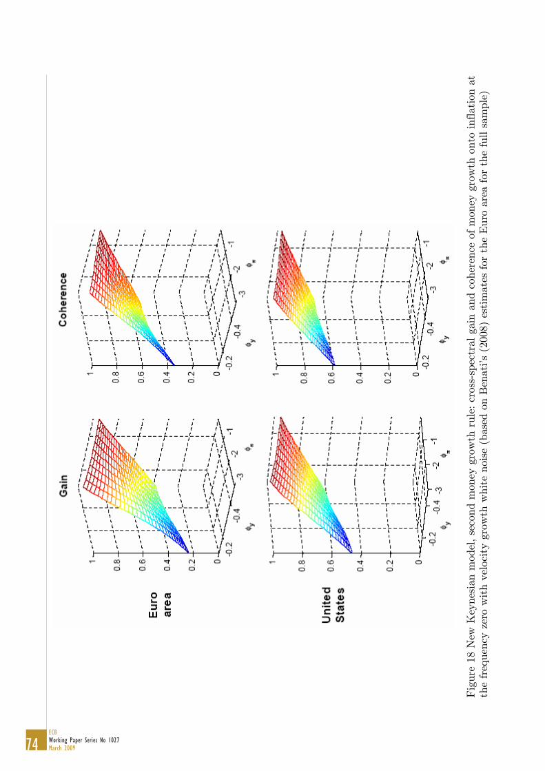
Fig

ure

18 N

ew K

eyne

sian

mod

el, se

cond

mon

ey g

r ow

th r

ule:

cro

ss-s

pect

ral ga

in a

nd c

oher

ence

of m

oney

gro

wth

ont

o in

flat

ion

at

the

freq

uenc

y ze

ro w

ith

velo

city

gro

wth

whi

te n

oise

(ba

sed

on B

enat

i’s (

2008

) es

tim

ates

for

the

Eur

o ar

ea for

the

ful

l sa

mpl

e)


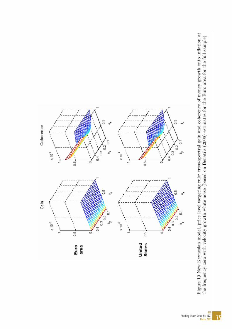
Fig

ure

19 N

ew K

eyne

sian

mod

el, pr

ice

leve

l ta

rget

ing

rule

: cr

oss-

spec

tral

gai

n an

d co

here

nce

of m

oney

gro

wth

ont

o in

flat

ion

at

the

freq

uenc

y ze

ro w

ith

velo

city

gro

wth

whi

te n

oise

(ba

sed

on B

enat

i’s (

2008

) es

tim

ates

for

the

Eur

o ar

ea for

the

ful

l sa

mpl

e)

75ECB


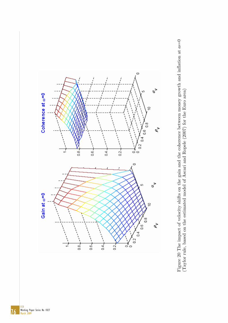
Fig

ure

20 T

he im

pact

of ve

loci

ty s

hif t

s on

the

gai

n an

d th

e co

here

nce

betw

een

mon

ey g

row

th a

nd inf

lati

on a

t ω

=0

(Tay

lor

rule

, ba

sed

on t

he e

stim

ated

mod

el o

f A

scar

i an

d R

opel

e (2

007)

for

the

Eur

o ar

ea)


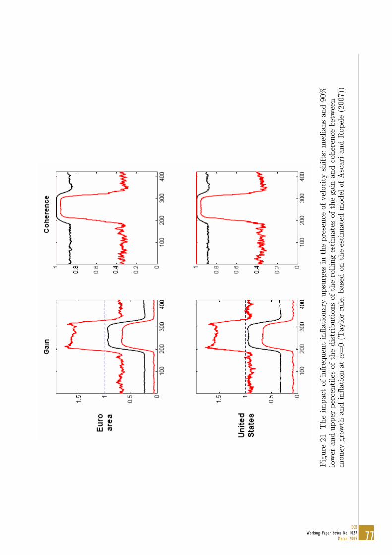
Fig

ure

21

The

im

pact

of in

freq

uent

inf

lati

onar

y up

surg

es in

the

pres

ence

of ve

loci

ty s

hift

s: m

edia

ns a

nd 9

0%

low

er a

nd u

pper

per

cent

iles

of t

he d

istr

ibut

ions

of th

e ro

lling

est

imat

es o

f th

e ga

in a

nd c

oher

ence

bet

wee

n m

oney

gro

wth

and

inf

lati

on a

t ω

=0

(Tay

lor

rule

, ba

sed

on t

he e

stim

ated

mod

el o

f A

scar

i an

d R

opel

e (2

007)

)

77ECB


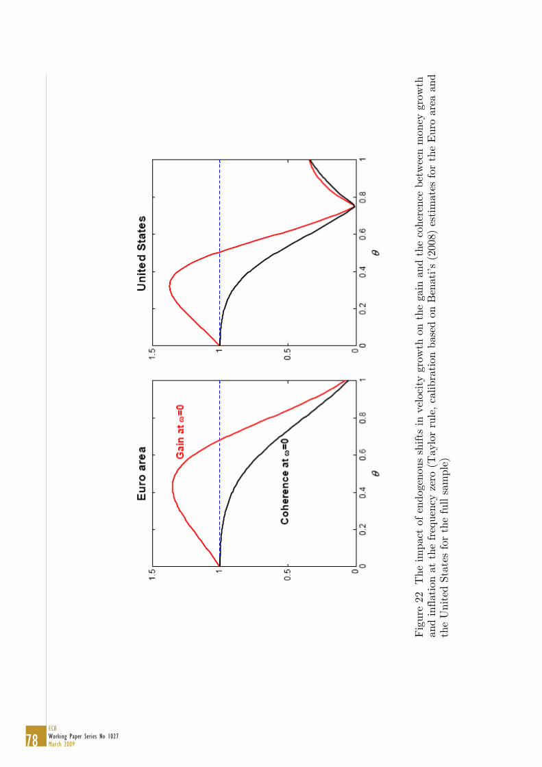
Fig

ure

22

The

im

pact

of en

doge

nous

shi

fts

in v

eloc

ity

grow

th o

n th

e ga

in a

nd t

he c

oher

ence

bet

wee

n m

oney

gro

wth

an

d in

flat

ion

at t

he fre

quen

cy z

ero

(Ta y

lor

rule

, ca

libra

tion

bas

ed o

n B

enat

i’s (

2008

) es

tim

ates

for

the

Eur

o ar

ea a

nd

the

Uni

ted

Stat

es for

the

ful

l sa

mpl

e)


79ECB


European Central Bank Working Paper Series

For a complete list of Working Papers published by the ECB, please visit the ECB’s website (http://www.ecb.europa.

eu).

973 “Do China and oil exporters influence major currency configurations?” by M. Fratzscher and A. Mehl,

December 2008.

974 “Institutional features of wage bargaining in 23 European countries, the US and Japan” by P. Du Caju, E. Gautier,

D. Momferatou and M. Ward-Warmedinger, December 2008.

975 “Early estimates of euro area real GDP growth: a bottom up approach from the production side” by E. Hahn

and F. Skudelny, December 2008.

976 “The term structure of interest rates across frequencies” by K. Assenmacher-Wesche and S. Gerlach,

December 2008.

977 “Predictions of short-term rates and the expectations hypothesis of the term structure of interest rates”

by M. Guidolin and D. L. Thornton, December 2008.

978 “Measuring monetary policy expectations from financial market instruments” by M. Joyce, J. Relleen and

S. Sorensen, December 2008.

979 “Futures contract rates as monetary policy forecasts” by G. Ferrero and A. Nobili, December 2008.

980 “Extracting market expectations from yield curves augmented by money market interest rates: the case of Japan”

by T. Nagano and N. Baba, December 2008.

981 “Why the effective price for money exceeds the policy rate in the ECB tenders?” by T. Välimäki,

December 2008.

982 “Modelling short-term interest rate spreads in the euro money market” by N. Cassola and C. Morana,

December 2008.

983 “What explains the spread between the euro overnight rate and the ECB’s policy rate?” by T. Linzert and

S. Schmidt, December 2008.

984 “The daily and policy-relevant liquidity effects” by D. L. Thornton, December 2008.

985 “Portuguese banks in the euro area market for daily funds” by L. Farinha and V. Gaspar, December 2008.

986 “The topology of the federal funds market” by M. L. Bech and E. Atalay, December 2008.

987 “Probability of informed trading on the euro overnight market rate: an update” by J. Idier and S. Nardelli,

December 2008.

988 “The interday and intraday patterns of the overnight market: evidence from an electronic platform”

by R. Beaupain and A. Durré, December 2008.

989 “Modelling loans to non-financial corporations in the euro area” by C. Kok Sørensen, D. Marqués Ibáñez and

C. Rossi, January 2009.

990 “Fiscal policy, housing and stock prices” by A. Afonso and R. M. Sousa, January 2009.

991 “The macroeconomic effects of fiscal policy” by A. Afonso and R. M. Sousa, January 2009.


992 “FDI and productivity convergence in central and eastern Europe: an industry-level investigation” by

M. Bijsterbosch and M. Kolasa, January 2009.

993 “Has emerging Asia decoupled? An analysis of production and trade linkages using the Asian international input-

output table” by G. Pula and T. A. Peltonen, January 2009.

994 “Fiscal sustainability and policy implications for the euro area” by F. Balassone, J. Cunha, G. Langenus, B. Manzke,

J. Pavot, D. Prammer and P. Tommasino, January 2009.

995 “Current account benchmarks for central and eastern Europe: a desperate search?” by M. Ca’ Zorzi, A. Chudik

and A. Dieppe, January 2009.

996 “What drives euro area break-even inflation rates?” by M. Ciccarelli and J. A. García, January 2009.

997 “Financing obstacles and growth: an analysis for euro area non-financial corporations” by C. Coluzzi, A. Ferrando

and C. Martinez-Carrascal, January 2009.

998 “Infinite-dimensional VARs and factor models” by A. Chudik and M. H. Pesaran, January 2009.

999 “Risk-adjusted forecasts of oil prices” by P. Pagano and M. Pisani, January 2009.

1000 “Wealth effects in emerging market economies” by T. A. Peltonen, R. M. Sousa and I. S. Vansteenkiste,

January 2009.

1001 “Identifying the elasticity of substitution with biased technical change” by M. A. León-Ledesma, P. McAdam and

A. Willman, January 2009.

1002 “Assessing portfolio credit risk changes in a sample of EU large and complex banking groups in reaction to

macroeconomic shocks” by O. Castrén, T. Fitzpatrick and M. Sydow, February 2009.

1003 “Real wages over the business cycle: OECD evidence from the time and frequency domains”

by J. Messina, C. Strozzi and J. Turunen, February 2009.

1004 “Characterising the inflation targeting regime in South Korea” by M. Sánchez, February 2009.

1005 “Labor market institutions and macroeconomic volatility in a panel of OECD countries” by F. Rumler and

J. Scharler, February 2009.

1006 “Understanding sectoral differences in downward real wage rigidity: workforce composition, institutions,

technology and competition” by P. Du Caju, C. Fuss and L. Wintr, February 2009.

1007 “Sequential bargaining in a new-Keynesian model with frictional unemployment and staggered wage negotiation”

by G. de Walque, O. Pierrard, H. Sneessens and R. Wouters, February 2009.

1008 “Liquidity (risk) concepts: definitions and interactions” by K. Nikolaou, February 2009.

1009 “Optimal sticky prices under rational inattention” by B. Maćkowiak and M. Wiederholt, February 2009.

K. Moll, February 2009.

1012 “Petrodollars and imports of oil exporting countries” by R. Beck and A. Kamps, February 2009.

1010 “Business cycles in the euro area” by D. Giannone, M. Lenza and L Reichlin, February 2009.

1011 “The global dimension of inflation – evidence from factor-augmented Phillips curves” by S. Eickmeier and

1013 “Structural breaks, cointegration and the Fisher effect” by A. Beyer, A. A. Haug and B. Dewald, February 2009.

81ECB


1014 “Asset prices and current account fluctuations in G7 economies” by M. Fratzscher and R. Straub, February 2009.

February 2009.

1016 “When does lumpy factor adjustment matter for aggregate dynamics?” by S. Fahr and F. Yao, March 2009.

1017 “Optimal prediction pools” by J. Geweke and G. Amisano, March 2009.

1018 “Cross-border mergers and acquisitions: financial and institutional forces” by N. Coeurdacier, R. A. De Santis

and A. Aviat, March 2009.

1019 “What drives return to euro area housing? Evidence from a dynamic divided-discount model” by P. Hiebert and

M. Sydow, March 2009.

by A. Beyer, V. Gaspar, C. Gerberding and O. Issing, March 2009.

1021 “Rigid labour compensation and flexible employment? Firm-level evidence with regard to productivity for

Belgium” by C. Fuss and L. Wintr, March 2009.

1022 “Understanding inter-industry wage structures in the euro area” by V. Genre, K. Kohn and D. Momferatou,

March 2009.

1023 “Bank loan announcements and borrower stock returns: does bank origin matter?” by S. Ongena and

V. Roscovan, March 2009.

1024 “Funding liquidity risk: definition and measurement” by M. Drehmann and K. Nikolaou, March 2009.

1025 “Liquidity risk premia in unsecured interbank money markets” by J. Eisenschmidt and J. Tapking, March 2009.

1026 “Do house price developments spill over across euro area countries? Evidence from a global VAR”

by I. Vansteenkiste and P. Hiebert, March 2009.

1027 “Long run evidence on money growth and inflation” by L. Benati, March 2009.

1015 “Inflation forecasting in the new EU Member States” by O. Arratibel, C. Kamps and N. Leiner-Killinger,

1020 “Opting out of the Great Inflation: German monetary policy after the break down of Bretton Woods”

by Olli Castren, Trevor Fitzpatrick and Matthias Sydow

Assessing Portfolio Credit risk ChAnges in A sAmPle of eU lArge And ComPlex BAnking groUPs in reACtion to mACroeConomiC shoCks

Work ing PAPer ser i e sno 1002 / f eBrUAry 2009

Date post:	13-Sep-2018
Category:	Documents
Upload:	vuongkiet
View:	216 times
Download:	0 times

Long run evidence on money growth and inflation · by Luca Benati Long Run EvidEncE on MonEy gRowth...

Documents