Long-term estimates of the energy-return-on-investment

(EROI) of coal, oil, and gas global productions

Victor COURTa,b,c and Florian FIZAINEd

a EconomiX, UMR 7235, UPL, Univ. Paris Nanterre, 200 avenue de la République, 92001 Nanterre, France. b IFP Energies Nouvelles, 1-4 avenue du Bois Préau, 92852 Rueil-Malmaison, France. c Chaire Economie du Climat, Palais Brongniart, 28 place de la Bourse, 75002 Paris, France. d LEDi - Laboratoire d'Économie de Dijon, Univ. Bourgogne Franche Comté, 2 Boulevard Gabriel, 21066 Dijon,

France.

Abstract

We use a price-based methodology to assess the global energy-return-on-investment

(EROI) of coal, oil, and gas, from the beginning of their reported production (respectively

1800, 1860, and 1890) to 2012. It appears that the EROI of global oil and gas productions

reached their maximum values in the 1930s–40s, respectively around 50:1 and 150:1, and

have declined subsequently. Furthermore, we suggest that the EROI of global coal production

has not yet reached its maximum value. Based on the original work of Dale et al. (2011), we

then present a new theoretical dynamic expression of the EROI. Modifications of the original

model were needed in order to perform calibrations on each of our price-based historical

estimates of coal, oil, and gas global EROI. Theoretical models replicate the fact that

maximum EROIs of global oil and gas productions have both already been reached while this

is not the case for coal. In a prospective exercise, the models show the pace of the expected

EROIs decrease for oil and gas in the coming century. Regarding coal, models are helpful to

estimate the value and date of the EROI peak, which will most likely occur between 2025 and

2045, around a value of 95(±15):1.

Key words: fossil fuel prices, fossil fuel EROIs, theoretical EROI function.

JEL classification: N7, Q3, Q4, Q5.

E-mail adresses: victorcourt@free.fr, florian.fizaine@gmail.com.

2

1. Introduction

1.1 Biophysical economics

The perception of the human society as a biophysical system has been expressed in

the pioneering works of Odum (1971; 1973), Georgescu-Roegen (1971; 1979), Cleveland et

al. (1984) and more recently by Ayres & Warr (2009), Kümmel (2011) and Hall & Klitgaard

(2012). In order to support calls for a broad paradigm shift in economics (Faber et al. 1987;

Hall et al. 2001; Hall & Klitgaard 2006), biophysical approaches of the economy have been

developed in pure conceptual papers related to entropy and sustainability (Perrings 1987;

O’Connor 1991; Ayres 1998; Krysiak 2006). From a more practical point of view, this stream

of thought has been represented by the energy science literature (input/output analysis, energy

and mass flows accounting, etc.) that started at the same time. In particular, the energy-return-

on-investment (EROI) has attracted considerable attention since all organisms or systems

need to procure at least as much energy as they consume in order to pursue their existence.

The EROI is the ratio of the quantity of energy delivered by a given process to the quantity of

energy consumed in this same process. Hence, the EROI is a measure of the accessibility of a

resource, meaning that the higher the EROI, the greater the amount of net energy delivered to

society in order to support economic growth (Hall et al. 2014). To the partisans of biophysical

economics, it leaves no doubt that the development of industrial societies has been largely

dependent on fossil fuels, and in particular on their high EROIs and consequent capacity to

deliver large amounts of net energy to society.

1.2 EROI of energy systems and implications for society

Because of the lack of hindsight regarding renewables and unconventional fossil fuels

(such as shale oil, heavy oil, tar sands, shale gas, etc.), time-series of EROI have been

calculated only for conventional fossil fuels resources and at national scales.1 The only EROI

study of international scope is the one of Gagnon et al. (2009) concerning the global oil and

gas production between 1992 and 2006. Furthermore, EROI time series are most of the time

computed on short or mid-term time horizons (a few decades at most). A notable exception to

this fact is the EROI assessment of the United States oil and gas industry from 1919 to 2007

performed by Guilford et al. (2011). The results of all these different studies are synthetized

in Hall et al. (2014). They all show declining trends during recent decades with maximum

EROI reached in the past. As society necessarily turns towards lower quality of conventional

and unconventional fossil fuels, more and more energy is invested in the energy-extraction

sub-system of the economy, making net energy delivered to society less available and fuels

more expensive in the long run. For these reasons, but mostly for geostrategic reasons and the

pollution associated with the use of fossil fuels, political and scientific attention is

increasingly being paid to renewable sources of energy. Unfortunately, EROI analyses have

shown that so far, renewable technologies do not generate as much net energy as fossil energy

used to (Murphy & Hall 2010; Hall et al. 2014). Furthermore, as stated by Fizaine & Court

(2015), the EROI of renewable electricity producing technologies is more sensitive that of

fossil fuels to the increasing energy cost associated with the extraction of the numerous

1 Time series of fossil fuels EROI found in the literature review of Hall et al. (2014) concern the following productions: United

States oil and gas, Canadian oil and gas, Norwegian oil and gas, Mexican oil and gas, Chinese oil, gas and coal, Canadian dry gas

and United States dry gas.

3

common and geologically rare metals required in their construction. Hence, for now,

performing an energy transition towards renewable technologies seems to necessarily imply a

shift from a higher to a lower EROI supply energy mix (i.e. a decrease of the societal EROI).

The consequences of this pattern on society remain unclear, but it necessarily raises some

serious concerns since our complex, industrialized societies have been built on the use of high

quality fossil energy resources, and that the dependence of the economy on its fossil energy

supply could potentially have huge adverse effects on its capacity for development (Court et

al. 2017).

1.3 Missing perspective, goal, and content

These facts have already been discussed in broader discussions regarding the potential for

long-term sustainable development of modern societies (Hall & Day 2009; Hall et al. 2009;

Murphy & Hall 2010; 2011a; 2011b; Lambert et al. 2014); but it is worth emphasizing that

the EROI of the different fossil energy types used in the economy have never been formally

estimated from their respective starting time of production to the present. To achieve such a

goal, we use in the current paper a methodology based on the relation of inflation-corrected

price and EROI, as first given in King & Hall (2011). Our methodology delivers estimates of

the global EROI of coal, oil, and gas, from the beginning of their reported production

(respectively 1800, 1860, and 1890) to 2012. In order to do that, we have first had to recover

different coherent time-series for the same time periods, concerning:

the energy prices of the different fossil energy types,

the global primary energy mix,

the monetary-return-on-investment of the energy sector or MROI (i.e. the gross

margin equals to “1 + the gross margin rate”; meaning that if the gross margin rate is

20%, the corresponding MROI is 1.2),

the energy intensity of capital expenditures in the primary fossil energy sector.

These data estimations allowed us to compute an average price of fossil energy weighted by

the quantities of produced fossil energy from 1800 to 2012, and to subsequently build time-

series estimates of the global EROI of the diverse fossil energy resources (coal, oil, and gas)

and of the global primary fossil energy system over the same time period. The methodology

employed to compute the time-series of energy prices and EROI of the different fossil energy

resources and finally estimate the EROI of the global primary fossil energy system are

presented in Section 2. In this section we also propose a new theoretical dynamic expression

of the EROI of a given energy resource as a function of its cumulated production, based on

the original work of Dale et al. (2011). The results of the price-based EROI estimates of

global coal, oil, and gas productions are presented and commented in Section 3. While some

of our results clearly support educated guesses advanced in previous papers about global oil

and gas (namely, that their maximum EROI has already been reached in the past), our results

regarding global coal EROI are quite innovative and counterintuitive. We then confront these

historical price-based estimates to the theoretical EROI models elaborated from the original

work of Dale et al. (2011). In Section 4, we discuss some biases of our methodology and

assess the robustness of our results with a comparison to previous existing studies. Finally, in

Section 5, we conclude and propose some research perspectives which would be worth

investigating as an extension of the present work.

4

2. Methods

2.1 Price-based estimation of historical fossil fuels global EROI

System boundary

Before specifying our methodology, we follow King et al. (2015) to highlight that the

EROI we estimate in this article should be more properly conceptualized as a “Gross Power

Return Ratio” since it represents the ratio of annual gross energy produced to annual energy

invested. In the strict meaning of the term, the global EROI of a given fossil fuel (expressed

as the ratio of cumulated energy production to total energy invested) will be computable only

once the last unit of this fossil energy will be extracted from the Earth. Hence, in the present

study we estimate annual (or “yearly”) EROIs, which thus abstract from the fact that some of

this year's production is from prior year's investments, and some of this year's investment will

result in future production. We used the EROI denomination for convenience but we

recommend the reader to consult the work of King et al. (2015) to get things straight on the

various computable energy ratios that exist and the way they relate to each other.

Regarding the output boundary of our study, it is clear considering our methodology

that the different EROIs we estimate are all at the mine-mouth or well-head since they

concern primary fossil energy. Concerning the input boundary of our study, since we rely on a

price-based approach, it makes sense to think that such a price of primary fossil energy

covers: direct energy expenditures, indirect energy expenditures from physical capital

investment, and indirect energy embodied in what workers purchase with their paycheck (i.e.

the energy used to provide food, shelter, transport, and all other things consumed by workers)

since wages paid to workers in the energy sector are covered by energy prices. As a

consequence, if we refer to the nomenclature of Murphy et al. (2011), the different energy

ratios we estimate in this article correspond to “annual EROI1,labor”.

Equations

Our methodology to estimate the EROI of global primary fossil energy system over

time is inspired by the work of King & Hall (2011). For a given year, the 𝐸𝑅𝑂𝐼𝑖 (unitless) of

the fossil energy sector, with 𝑖 ∈ (𝐶𝑜𝑎𝑙, 𝑂𝑖𝑙, 𝐺𝑎𝑠), can simply be expressed as the ratio of the

energy produced 𝐸𝑜𝑢𝑡,𝑖 (expressed in exajoule, or EJ) to the energy 𝐸𝑖𝑛,𝑖 (EJ) invested in the

energy sector i:

𝐸𝑅𝑂𝐼𝑖 =𝐸𝑜𝑢𝑡,𝑖

𝐸𝑖𝑛,𝑖

. (1)

Estimating the i different energy output 𝐸𝑜𝑢𝑡,𝑖 is rather simple since databases for coal, oil,

and gas historical productions are quite reliable. On the other hand, estimating the energy

𝐸𝑖𝑛,𝑖 invested in each energy sector is far more difficult, especially in long-term analyses.

Regarding the global economy, it can be proposed that the energy 𝐸𝑖𝑛,𝑖 (EJ) invested in the

global energy system i corresponds to the quantity of money 𝑀𝑖𝑛,𝑖 (expressed in million

International Geary-Khamis 1990 dollar,2 or M$1990) invested in this sector multiplied by the

average energy intensity 𝐸𝐼𝑖 (EJ/M$1990) of capital and services installed and used in the

2 The International Geary-Khamis 1990 dollar, more commonly known as the international dollar (properly abbreviated Int. G-K.

$1990, and more simply $1990 in this study), is a standardized and fictive unit of currency that has the same purchasing power

parity as the U.S. dollar had in the United States in 1990.

5

energy sector i (i.e. the direct energy consumption of the energy sector i, plus the indirect

quantity of energy consumed by the economic system to generate a unitary dollar

consequently spent as capital and services installation and use in this same energy sector).

Hence, (1) is rearranged as

𝐸𝑅𝑂𝐼𝑖 =𝐸𝑜𝑢𝑡,𝑖

𝑀𝑖𝑛,𝑖 ∗ 𝐸𝐼𝑖

. (2)

Of course, the problem now lies in estimating the quantity of money 𝑀𝑖𝑛,𝑖 invested in the

global energy sector for which very few data exist. Thus, we assume that the unitary price 𝑃𝑖

(M$1990/EJ) of a given energy type divided by the monetary-return-on-investment or 𝑀𝑅𝑂𝐼𝑖

(unitless) of the energy sector i is a proxy for 𝐶𝑝𝑟𝑜𝑑,𝑖 , the annual (and not levelized)

production cost of this same energy. This allows us to estimate the total money 𝑀𝑖𝑛,𝑖 invested

in a given energy sector by multiplying the quantity of energy produced 𝐸𝑜𝑢𝑡,𝑖 by this sector

with the proxy annual cost of this same energy:

𝑀𝑖𝑛,𝑖 = 𝐶𝑝𝑟𝑜𝑑,𝑖 ∗ 𝐸𝑜𝑢𝑡,𝑖 =𝑃𝑖

𝑀𝑅𝑂𝐼𝑖

∗ 𝐸𝑜𝑢𝑡,𝑖 . (3)

By injecting (3) into (2), we obtain that, for each year, the estimated 𝐸𝑅𝑂𝐼𝑖 at global level is

𝐸𝑅𝑂𝐼𝑖 =𝑀𝑅𝑂𝐼𝑖

𝑃𝑖 ∗ 𝐸𝐼𝑖

. (4)

Due to data availability, we have to make two further important assumptions. First, the

𝑀𝑅𝑂𝐼𝑖 of all i energy sectors are the same and correspond to an average MROI of the fossil

energy sector. In Section 4.1, we test three different possibilities to estimate this MROI. They

deliver very similar results and show that our EROI estimates are almost insensitive to the

MROI because the influence of the price and the energy intensity are far more important.

Second, the energy intensities 𝐸𝐼𝑖 of all i energy sectors are the same and correspond to the

average energy intensity EI of the global economy. In the discussion of Section 4.1, we also

test the sensitivity of our results to this assumption because it is very likely that the different

expenditures of the global fossil energy sector present an overall higher energy intensity than

the average expenditures of the global economy. The global energy intensity EI logically

evolves over time and it can be easily computed for a given year as

𝐸𝐼 =∑ 𝐸𝑜𝑢𝑡,𝑗𝑗

𝐺𝑊𝑃, 𝑗 ∈ (𝐶𝑜𝑎𝑙, 𝑂𝑖𝑙, 𝐺𝑎𝑠, 𝑁𝑢𝑐𝑙𝑒𝑎𝑟, 𝐴𝑙𝑙 𝑟𝑒𝑛𝑒𝑤𝑎𝑏𝑙𝑒𝑠) (5)

where 𝐺𝑊𝑃 (M$1990) is the gross world product. As shown in (5), in order to calculate the

variable EI, we have to include the other quantities of energy productions coming from

nuclear and renewable energy forms (wind, solar, geothermic, ocean, biofuels, wood, wastes).

It follows from these assumptions that (4) becomes

𝐸𝑅𝑂𝐼𝑖 =𝑀𝑅𝑂𝐼

𝑃𝑖 ∗ 𝐸𝐼. (6)

6

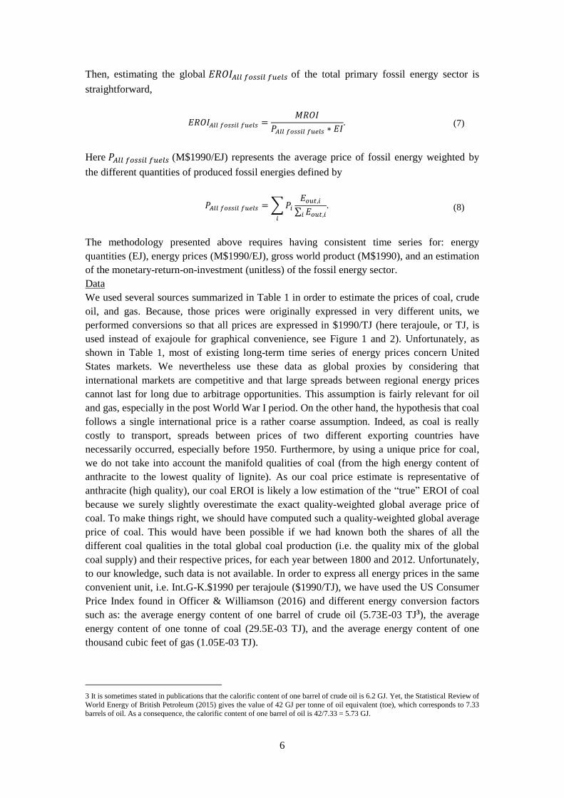
Then, estimating the global 𝐸𝑅𝑂𝐼𝐴𝑙𝑙 𝑓𝑜𝑠𝑠𝑖𝑙 𝑓𝑢𝑒𝑙𝑠 of the total primary fossil energy sector is

straightforward,

𝐸𝑅𝑂𝐼𝐴𝑙𝑙 𝑓𝑜𝑠𝑠𝑖𝑙 𝑓𝑢𝑒𝑙𝑠 =𝑀𝑅𝑂𝐼

𝑃𝐴𝑙𝑙 𝑓𝑜𝑠𝑠𝑖𝑙 𝑓𝑢𝑒𝑙𝑠 ∗ 𝐸𝐼. (7)

Here 𝑃𝐴𝑙𝑙 𝑓𝑜𝑠𝑠𝑖𝑙 𝑓𝑢𝑒𝑙𝑠 (M$1990/EJ) represents the average price of fossil energy weighted by

the different quantities of produced fossil energies defined by

𝑃𝐴𝑙𝑙 𝑓𝑜𝑠𝑠𝑖𝑙 𝑓𝑢𝑒𝑙𝑠 = ∑ 𝑃𝑖

𝑖

𝐸𝑜𝑢𝑡,𝑖

∑ 𝐸𝑜𝑢𝑡,𝑖𝑖

. (8)

The methodology presented above requires having consistent time series for: energy

quantities (EJ), energy prices (M$1990/EJ), gross world product (M$1990), and an estimation

of the monetary-return-on-investment (unitless) of the fossil energy sector.

Data

We used several sources summarized in Table 1 in order to estimate the prices of coal, crude

oil, and gas. Because, those prices were originally expressed in very different units, we

performed conversions so that all prices are expressed in $1990/TJ (here terajoule, or TJ, is

used instead of exajoule for graphical convenience, see Figure 1 and 2). Unfortunately, as

shown in Table 1, most of existing long-term time series of energy prices concern United

States markets. We nevertheless use these data as global proxies by considering that

international markets are competitive and that large spreads between regional energy prices

cannot last for long due to arbitrage opportunities. This assumption is fairly relevant for oil

and gas, especially in the post World War I period. On the other hand, the hypothesis that coal

follows a single international price is a rather coarse assumption. Indeed, as coal is really

costly to transport, spreads between prices of two different exporting countries have

necessarily occurred, especially before 1950. Furthermore, by using a unique price for coal,

we do not take into account the manifold qualities of coal (from the high energy content of

anthracite to the lowest quality of lignite). As our coal price estimate is representative of

anthracite (high quality), our coal EROI is likely a low estimation of the “true” EROI of coal

because we surely slightly overestimate the exact quality-weighted global average price of

coal. To make things right, we should have computed such a quality-weighted global average

price of coal. This would have been possible if we had known both the shares of all the

different coal qualities in the total global coal production (i.e. the quality mix of the global

coal supply) and their respective prices, for each year between 1800 and 2012. Unfortunately,

to our knowledge, such data is not available. In order to express all energy prices in the same

convenient unit, i.e. Int.G-K.$1990 per terajoule ($1990/TJ), we have used the US Consumer

Price Index found in Officer & Williamson (2016) and different energy conversion factors

such as: the average energy content of one barrel of crude oil (5.73E-03 TJ3), the average

energy content of one tonne of coal (29.5E-03 TJ), and the average energy content of one

thousand cubic feet of gas (1.05E-03 TJ).

3 It is sometimes stated in publications that the calorific content of one barrel of crude oil is 6.2 GJ. Yet, the Statistical Review of

World Energy of British Petroleum (2015) gives the value of 42 GJ per tonne of oil equivalent (toe), which corresponds to 7.33

barrels of oil. As a consequence, the calorific content of one barrel of oil is 42/7.33 = 5.73 GJ.

7

Table 1. Sources and original units of the different energy prices used in this study.

Energy Time and spatial coverage Source Original unit

Coal 1800–2012: US average

anthracite price.

US Bureau of the Census (1975, pp.207–209)

from 1800 to 1948. EIA (2012, p.215) from

1949 to 2011. EIA (2013, p.54) for 2012.

Nominal $/80-lb

from 1800 to

1824, then

nominal $/short

ton.4

Oil 1860–1944: US average;

1945–1983: Arabian Light

posted at Ras Tanura;

1984–2012: dated Brent.

British Petroleum (2015) for the entire period. Nominal $/barrel.

Gas 1890–2012: US average

price at the wellhead.

US Bureau of the Census (1975, pp.582–583)

from 1890 to 1915. Manthy (1978, p.111)

from 1916 to 1921. EIA (2016, p.145) from

1922 to 2012.

Nominal

$/thousand cubic

feet.

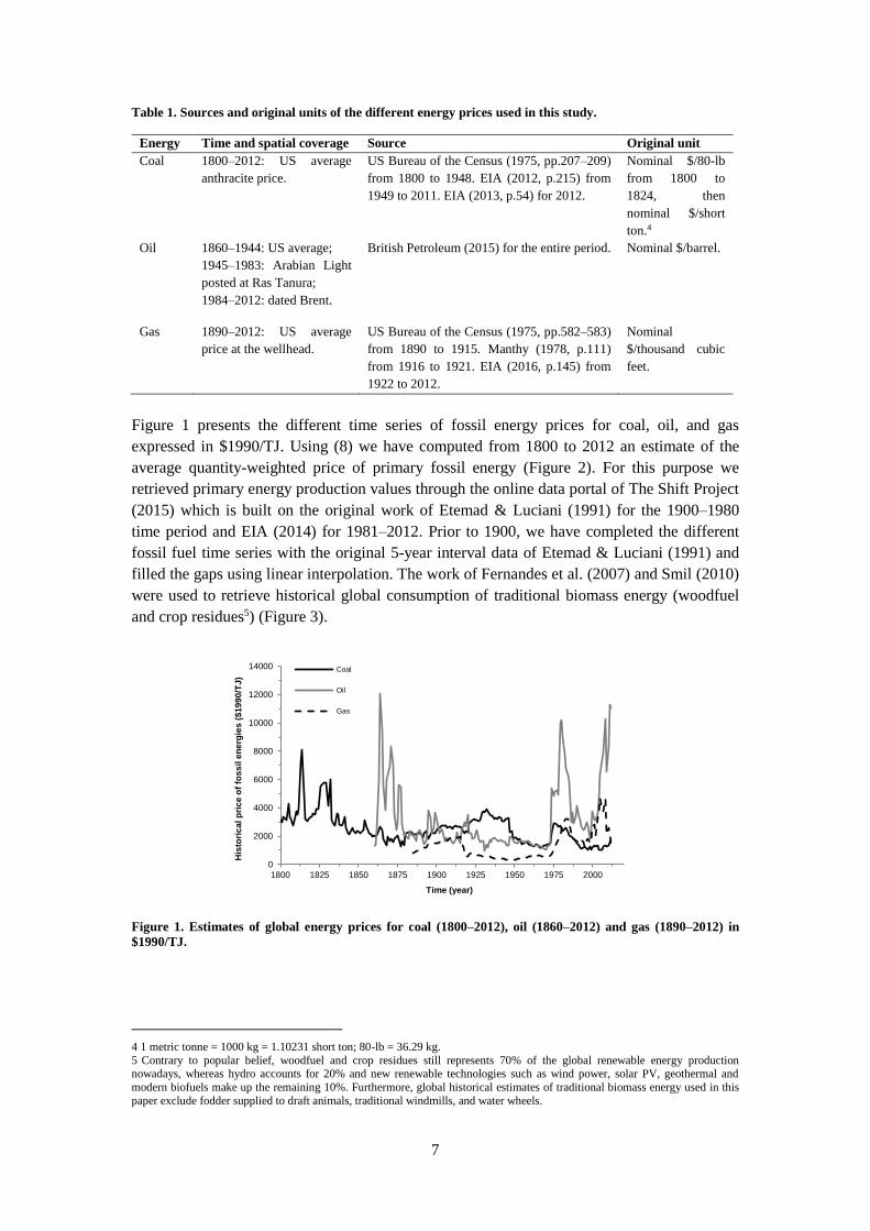
Figure 1 presents the different time series of fossil energy prices for coal, oil, and gas

expressed in $1990/TJ. Using (8) we have computed from 1800 to 2012 an estimate of the

average quantity-weighted price of primary fossil energy (Figure 2). For this purpose we

retrieved primary energy production values through the online data portal of The Shift Project

(2015) which is built on the original work of Etemad & Luciani (1991) for the 1900–1980

time period and EIA (2014) for 1981–2012. Prior to 1900, we have completed the different

fossil fuel time series with the original 5-year interval data of Etemad & Luciani (1991) and

filled the gaps using linear interpolation. The work of Fernandes et al. (2007) and Smil (2010)

were used to retrieve historical global consumption of traditional biomass energy (woodfuel

and crop residues5) (Figure 3).

Figure 1. Estimates of global energy prices for coal (1800–2012), oil (1860–2012) and gas (1890–2012) in

$1990/TJ.

4 1 metric tonne = 1000 kg = 1.10231 short ton; 80-lb = 36.29 kg.

5 Contrary to popular belief, woodfuel and crop residues still represents 70% of the global renewable energy production nowadays, whereas hydro accounts for 20% and new renewable technologies such as wind power, solar PV, geothermal and

modern biofuels make up the remaining 10%. Furthermore, global historical estimates of traditional biomass energy used in this

paper exclude fodder supplied to draft animals, traditional windmills, and water wheels.

0

2000

4000

6000

8000

10000

12000

14000

1800 1825 1850 1875 1900 1925 1950 1975 2000

His

tori

ca

l p

ric

e o

f fo

ss

il e

ne

rgie

s (

$1

99

0/T

J)

Time (year)

Coal

Oil

Gas

8

Figure 2. Estimation of the global average quantity-weighted price of fossil energy in $1990/TJ, 1800–2012.

Figure 3. Global annual energy productions (EJ/year), 1800–2012. Data sources: Etemad & Luciani (1991),

Fernandes et al. (2007), Smil (2010), EIA (2014), The Shift project (2015).

The gross world product (GWP) of Figure 4 comes from Maddison (2007) from 1800

to 1950 and from the GWP per capita of The Maddison Project (2013) multiplied by the

United Nations (2015) estimates of global population from 1950 to 2010. In order to obtain

GWP estimates for 2011 and 2012 we used the real GWP growth rate of the World Bank

(2016). Dividing the GWP of Figure 4 by the sum of the primary energy productions of

Figure 3 yields the average energy intensity of the global economy presented in Figure 5

(expressed here for convenience in MJ per Int. G-K. $1990). We also present in Figure 5 the

energy intensity of the global economy over time when the consumption of traditional

biomass energy (woodfuel, crop residues) is not accounted for as seen in some studies (e.g.

Rühl et al. 2012). To our mind, not taking into account traditional biomass energy in the

calculation of a macroeconomic energy intensity is an important mistake. Finally, we follow

Damodaran (2015) who claims that the US fossil energy sector monetary-return-on-

investment (MROI) roughly follows the US long-term interest rate (US.LTIR retrieved from

Officer 2016) with a 10% risk premium. Hence, we compute the MROI of Figure 6 following:

𝑀𝑅𝑂𝐼 = 1 + ((𝑈𝑆. 𝐿𝑇𝐼𝑅 + 10)/100) (9)

0

1000

2000

3000

4000

5000

6000

7000

8000

9000

1800 1830 1860 1890 1920 1950 1980 2010

His

tori

ca

l a

ve

rag

e q

ua

nti

ty-w

eig

hte

d p

ric

e o

f fo

ss

il e

ne

rgy

($1

99

0/T

J)

Time (year)

0

25

50

75

100

125

150

175

200

1800 1820 1840 1860 1880 1900 1920 1940 1960 1980 2000

Glo

ba

l a

nn

ua

l e

ne

rgy p

rod

uc

tio

n (

EJ

/ye

ar)

Time (year)

Coal

Oil

Gas

Nuclear

Hydro

Other renewable electricity (wind, solar,geothermal, wastes, wave&tidal)

Biomass energy (woodfuel, crop residues,modern biofuels)

9

Figure 4. Gross world product (GWP) in billion international Geary–Khamis 1990 dollars, 1800–2012. Data

sources: Maddison (2007), The Maddison Project (2013), United Nations (2015), World Bank (2016).

Figure 5. Comparison of the energy intensity of the global economy over time (MJ/Int. G-K.$1990) when

traditional biomass energy (woodfuel, crop residues) is accounted for or not, 1800–2012.

Figure 6. Estimated average annual MROI of US energy sector, 1800–2012. Data source: Officer (2016).

0

10 000

20 000

30 000

40 000

50 000

60 000

1800 1830 1860 1890 1920 1950 1980 2010

His

tori

ca

l G

WP

(B

illi

on

In

t.G

-K.$

19

90

/ye

ar)

Time (year)

0

5

10

15

20

25

30

35

1800 1830 1860 1890 1920 1950 1980 2010

En

erg

y I

nte

ns

ity o

f th

e g

lob

al e

co

no

my

(MJ

/In

t. G

-K.$

19

90

)

Time (year)

Considering all energy flows

Omitting traditional biomass energy(wood, crop residues) as seen inRühl et al. (2012)

1,1

1,12

1,14

1,16

1,18

1,2

1,22

1,24

1800 1830 1860 1890 1920 1950 1980 2010

An

nu

al

MR

OI

(Dim

en

sio

nle

ss

)

Time (year)

10

2.2 A new theoretical dynamic model of EROI as a function of cumulated production

Dale et al. (2011) have proposed a dynamic expression of the EROI of a given energy

resource as a function of its utilization. Despite the use of such a functional expression of the

EROI in a broader theoretical model called GEMBA (Dale et al. 2012), the accuracy of this

theoretical model compared to historical EROI estimates of fossil fuels has never been tested.

Since in Section 3.1 we provide such global estimates for the EROI of coal, oil, and gas from

their respective beginnings of production to present time, we can compare these results with

the original theoretical model of Dale et al. (2011). In trying to do so, we found that this

theoretical model needed to be slightly modified in order to correct two drawbacks.

Theoretical considerations

Like Dale et al. (2011) we assume that, for a given year, the annual 𝐸𝑅𝑂𝐼𝑗 of a given

energy resource 𝑗 (either nonrenewable or renewable) depends on a scaling factor 𝜀𝑗, which

represents the maximum potential EROI value (never formally attained); and on a function

F(𝜌𝑗) depending on the exploited resource ratio 0 ≤ 𝜌𝑗 ≤ 1. In the case of nonrenewable

energy (but not renewable), 𝜌𝑗 is also known as the normalized cumulated production, i.e. the

cumulated production 𝐶𝑢𝑚𝐸𝑜𝑢𝑡,𝑗 normalized to the size of the Ultimately Recoverable

Resource6 𝑈𝑅𝑅𝑗 defined as the total resource that may be recovered at positive net energy

yield, i.e. at EROI greater or equal to unity.

𝜌𝑗(𝑛𝑜𝑛𝑟𝑒𝑛𝑒𝑤𝑎𝑏𝑙𝑒) = 𝐶𝑢𝑚𝐸𝑜𝑢𝑡,𝑗

𝑈𝑅𝑅𝑗

∈ [0,1]. (10)

As shown in (11), F(𝜌𝑗 ) is the product of two functions, G(𝜌𝑗 ) and H(𝜌𝑗 ). G(𝜌𝑗 ) is a

technological component that increases energy returns as a function of 𝜌𝑗, which here serves

as a proxy measure of experience, i.e. technological learning. H(𝜌𝑗) is a physical component

that diminishes energy returns because of a decline in the quality of the resource as 𝜌𝑗

increases towards 1 (i.e. as the resource is depleted):

𝐸𝑅𝑂𝐼𝑗(𝜌𝑗) = 𝜀𝑗𝐹(𝜌𝑗) = 𝜀𝑗𝐺(𝜌𝑗)𝐻(𝜌𝑗). (11)

Technological component G(𝜌𝑗)

In Dale et al. (2011) the technological component 𝐺(𝜌𝑗) is a strictly concave function

that increases with the exploited resource ratio 𝜌𝑗. We replace this formulation by a sigmoid

increasing functional form (S-shaped curve) that is more in accordance with the historical

technological improvements observed by Smil (2005) in the energy industry. Such a

formulation is thus convex at the beginning of the resource exploitation, reaches an inflexion

point, and then tends asymptotically towards a strictly positive upper limit (Figure 7). Hence,

6 According to British Petroleum (2015), the “URR is an estimate of the total amount of a given resource that will ever be

recovered and produced. It is a subjective estimate in the face of only partial information. Whilst some consider URR to be fixed by geology and the laws of physics, in practice estimates of URR continue to be increased as knowledge grows, technology

advances and economics change. The ultimately recoverable resource is typically broken down into three main categories:

cumulative production, discovered reserves and undiscovered resource”. On the other hand, Sorrell et al. (2010) highlight that unlike reserves, URR estimates are not dependent on technology assumptions and thus should only be determined by geologic

hypotheses. Unfortunately, this apparent contradiction of the URR definition is only a tiny example of the fuzziness of points of

view that one could find in the literature regarding the different notions of nonrenewable resources and reserves.

11

our formulation follows the precepts of the original 𝐺𝐷𝑎𝑙𝑒 𝑒𝑡 𝑎𝑙.(2011)(𝜌𝑗) component of

Dale et al. (2011): first, that there is some minimum amount of energy that must be embodied

in the energy extraction device; second, that there is a limit to how efficiently a device can

extract energy. In other words, we assume that as a technology matures, i.e. as experience is

gained, the processes involved become better equipped to use fewer resources (e.g. PV panels

and wind turbines become less energy intensive to produce, and more efficient in converting

primary energy into electricity). In our new formulation this technological learning is slow at

first and must endure a minimum learning time effort before taking off. Moreover, as in

Dale et al. (2011)’s original function, our formulation represents the fact that EROI increases

from technological improvements are subject to diminishing marginal returns up to a point

where processes approach fundamental theoretical limits (such as the Lancaster-Betz limit in

the case of wind turbines). In equation (12) we have reported the original functional

expression found in Dale et al. (2011) that we have called here 𝐺𝐷𝑎𝑙𝑒 𝑒𝑡 𝑎𝑙.(2011)(𝜌𝑗) in order

to make a distinction with (13) that is the function 𝐺(𝜌𝑗) that corresponds to the new

technological component of the EROI theoretical model.

𝐺𝐷𝑎𝑙𝑒 𝑒𝑡 𝑎𝑙.(2011)(𝜌𝑗) = 1 − Ψ𝑗exp(−𝜓𝑗𝜌𝑗). (12)

𝐺(𝜌𝑗) = Ψ𝑗 +1 − Ψ𝑗

1 + exp ( −𝜓𝑗(𝜌𝑗 − 𝜌��)). (13)

With 0 ≤ Ψ𝑗 < 1 representing the initial normalized EROI with the immature technology

used to start the exploitation of the energy source j. 𝜓𝑗 represents the constant rate of

technological learning through experience that depends on a number of both social and

physical factors that we do not represent. Finally in our new formulation, 𝜌�� is the particular

exploited resource ratio at which the growth rate of G(𝜌𝑗) is maximum (i.e. the particular

value of 𝜌𝑗 at which G(𝜌𝑗) presents its inflexion point).

Physical depletion component H(𝜌𝑗)

The physical resource component of the EROI function, H( 𝜌𝑗 ), is assumed to

decrease to an asymptotic limit as cumulated production increases. As advanced by Dale et al.

(2011), we follow the argument that on average production first comes from resources that

offer the best (financial or energy) returns before attention is turned towards resources

offering lower returns. Even if this is not completely true at a given moment and for a

particular investor, we think that such aggregated behavior, represented by (14), is consistent

with long-term economic rationality.7

𝐻(𝜌𝑗) = exp(−𝜑𝑗𝜌𝑗). (14)

Where 0 < 𝜑𝑗 represents the constant rate of quality degradation of the energy resource j. In

the original function of Dale et al. (2011), since there is no additional specification, the

7 A more detailed justification of the decreasing exponential functional form given to H( 𝜌𝑗 ), relying on the probability

distribution function of EROI among deposits of the same energy resource is available in Dale et al. (2011).

12

asymptotic limit of H(𝜌𝑗) is zero, which implies that ultimately energy deposits could be

exploited with an EROI inferior to unity (as represented in Figure 7). Such a production

choice could find some justification at national level as it is easy to imagine a country willing

to extract a strategic energy resource energy (such as crude oil for instance) with an EROI

inferior to unity thanks to another energy input with an EROI far above 1 (such as gas or

nuclear electricity for instance). But in a global and long-term future context, it does not make

much sense to think that the extraction of a nonrenewable energy resource with an EROI

inferior to one will last for long. Economic rationality implies that energy resources can

sporadically and locally be extracted with an EROI inferior to unity, but not in the long-run

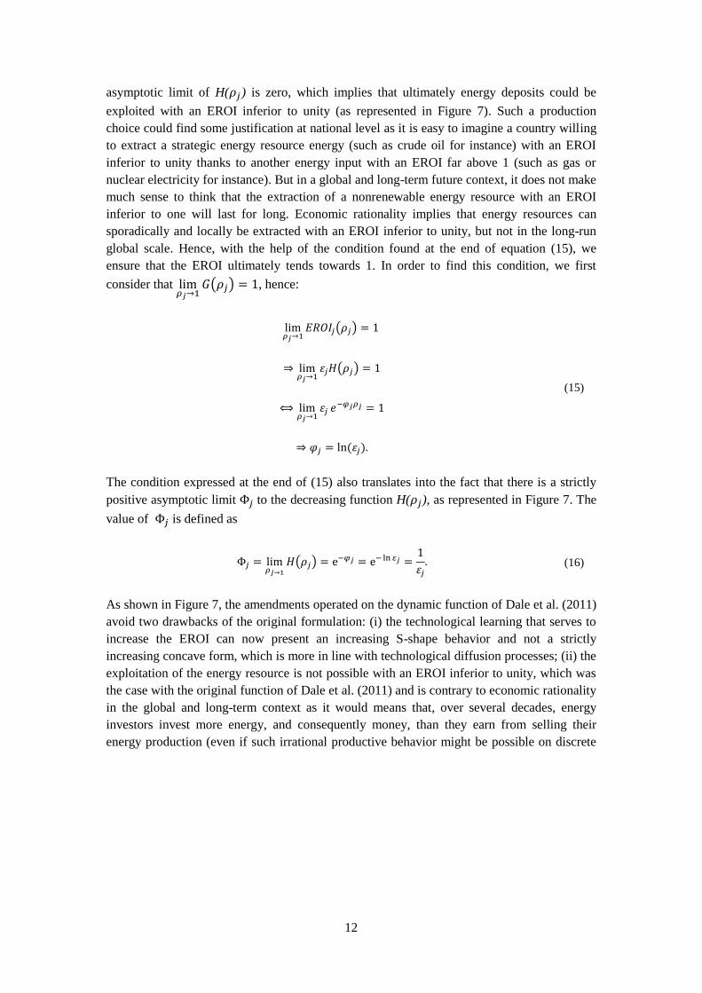
global scale. Hence, with the help of the condition found at the end of equation (15), we

ensure that the EROI ultimately tends towards 1. In order to find this condition, we first

consider that lim𝜌𝑗→1

𝐺(𝜌𝑗) = 1, hence:

lim𝜌𝑗→1

𝐸𝑅𝑂𝐼𝑗(𝜌𝑗) = 1

⇒ lim𝜌𝑗→1

𝜀𝑗𝐻(𝜌𝑗) = 1

⟺ lim𝜌𝑗→1

𝜀𝑗 𝑒−𝜑𝑗𝜌𝑗 = 1

⇒ 𝜑𝑗 = ln(𝜀𝑗).

(15)

The condition expressed at the end of (15) also translates into the fact that there is a strictly

positive asymptotic limit Φ𝑗 to the decreasing function H(𝜌𝑗), as represented in Figure 7. The

value of Φ𝑗 is defined as

Φ𝑗 = lim𝜌𝑗→1

𝐻(𝜌𝑗) = e−𝜑𝑗 = e− ln 𝜀𝑗 =1

𝜀𝑗

. (16)

As shown in Figure 7, the amendments operated on the dynamic function of Dale et al. (2011)

avoid two drawbacks of the original formulation: (i) the technological learning that serves to

increase the EROI can now present an increasing S-shape behavior and not a strictly

increasing concave form, which is more in line with technological diffusion processes; (ii) the

exploitation of the energy resource is not possible with an EROI inferior to unity, which was

the case with the original function of Dale et al. (2011) and is contrary to economic rationality

in the global and long-term context as it would means that, over several decades, energy

investors invest more energy, and consequently money, than they earn from selling their

energy production (even if such irrational productive behavior might be possible on discrete

13

production sites and for a short time).8 However, our new formulation of the theoretical

dynamic EROI function makes it more difficult to define the particular value of the exploited

resource ratio 𝜌𝐸𝑅𝑂𝐼𝑗 𝑚𝑎𝑥 at which the 𝐸𝑅𝑂𝐼𝑗 is maximum. This value cannot be found

arithmetically anymore (but numerical approximation is of course possible) because of the

new functional form we have introduced for the technological component G. Nevertheless, as

explained in the coming Section 3.2, the amendments brought to the original theoretical

model of Dale et al. (2011) were essential to allow its calibration to the historical price-based

estimates of the global EROI of coal, oil, and gas presented in Section 3.1.

Figure 7. Dale et al. (2011) vs. new (present article) functional forms for the theoretical EROI model.

In order to create historical estimates of global EROI for coal, oil, gas, and total fossil fuels

with the theoretical model previously presented, we first need to determine their respective

exploited resource ratios. Doing so implies defining the Ultimately Recoverable Resource

(URR) of each fossil resource. In the present paper, we define the URR of a given energy

8 A very important point that is not stressed in Dale et al. (2011) is that the dynamic function of the EROI does not represent the

same physical indicator if one considers a nonrenewable or a renewable energy resource. In the case of a nonrenewable energy resource, equation (11) and the right side of Figure 7 describe the average annual EROI with which the nonrenewable energy is

extracted from the environment. But in the case of renewable energy, equation (11) and the right side of Figure 7 describe the

marginal annual EROI with which the renewable energy is extracted from the environment. For example, if we take the example of oil for the nonrenewable energy resource, the dynamic EROI function described in this section implicates that the last barrel of

oil that will be extracted from the ground in the future will have an EROI just above 1. In the case of a renewable energy

resource such as wind, the same model means that the last wind turbine that will be installed, and will totally saturate the technical potential of wind energy, will have an EROI just above 1; but of course, in such a future situation the whole annual

production of energy from wind turbines will have an average EROI far above 1. This difference is not relevant for our paper, but

it is off course very important in the context of the energy transition.

��

New (present thesis) functional forms for the theoretical EROI model

Technological component 𝑮 Physical component 𝑯 Complete function 𝑭

EROI

𝝆

EROI of virgin resource

Strictly positive asymptotic value

𝚽

EROI

𝝆

Technological limit

Initial EROI with immature technology

1

𝚿

EROI

𝝆

Maximum potential EROI

Break even limit (EROI = 1)

𝛆

1

1 1 1

Dale et al. (2011) functional forms for the theoretical EROI model

EROI of virgin resource

Technological component 𝑮 Physical component 𝑯 Complete function 𝑭

1

𝚿

EROI

𝝆

Technological limit

Initial EROI with immature technology

EROI

𝝆

1

1

EROI

𝝆

Maximum potential EROI

Break even limit (EROI = 1)

𝛆

1

1 1

1

𝐻(𝜌) = 𝑒𝑥𝑝(−𝜑𝜌)

𝐻(𝜌) = 𝑒𝑥𝑝(−𝜑𝜌) and

𝜑 = 𝑙𝑛 (𝜀)

𝐺(𝜌) = 1 − 𝛹𝑒𝑥𝑝(−𝜓𝜌)

𝐺(𝜌) = 𝛹 +1 − 𝛹

1 + 𝑒𝑥𝑝 (−𝜓(𝜌 − ��))

14

resource as the total energy resource that may be recovered at positive net energy yield, i.e. at

EROI greater or equal to unity. These values, presented in Table 2, were retrieved from the

best estimates of McGlade & Ekins (2015) for oil (Gb: giga barrel), gas (Tcm: terra cubic

meters), and coal (Gt: giga tonnes), which for the record are in accordance with the last

IIASA Global Energy Assessment report (IIASA 2012). Regarding the coal URR, we found

much lower values in other studies, like the average estimate of 1150 Gt (corresponding to 29

500 EJ) given in the literature review of Mohr & Evans (2009). When compared to the order

of magnitude of 100 000 EJ found in McGlade & Ekins (2015) and IIASA (2012), lower

estimation of 29 500 EJ advanced by Mohr & Evans (2009) as an URR corresponds more,

according to us, to a proven reserve estimation. However, we will use this lower coal URR

estimate to test the sensitivity of our model to this crucial parameter in Section 4.3.

Table 2. Coal, oil, and gas global URR. Source: McGlade & Ekins, 2015.

Energy resource Global URR

(diverse units)

Conversion factors

(diverse units) Global URR* (EJ)

Coal 4085 (Gt) 105,000

63% hard coal 2565 (Gt) 32.5E-9 EJ/tonne 83,500

37% lignite coal 1520 (Gt) 14.0E-9 EJ/tonne 21,500

Oil 5070 (Gb) 29,000

Conventional oil 2615 (Gb) 5.73E-9 EJ/barrel 15,000

Unconventional oil 2455 (Gb) 5.73E-9 EJ/barrel 14,000

Gas 675 (Tcm) 27,000

Conventional gas 375 (Tcm) 40 EJ/Tcm 15,000

Unconventional gas 300 (Tcm) 40 EJ/Tcm 12,000

Total fossil fuels 161,000 *URR values expressed in EJ have been rounded up to the nearest 500.

3. Results

3.1 Price-based estimates of historical fossil fuels global EROI

Figure 8 presents the estimations of the global EROI of coal, oil, gas, and of the total

primary fossil energy system obtained with the price-based methodology developed in

Section 2.1. Separate graphical representations for each energy type are available in Figure 9.

Considering that our approach is based on financial data (prices, MROI) and that (in the

absence of any better solution) energy intensity was taken as the average of global society at

large, analyses of results shall retain orders of magnitude and trends and absolutely not

precise estimated values for given years. It is interesting to see that according to our estimates,

and contrary to what common sense would suggest, the global EROI of the three fossil fuels

(coal, oil, and gas) were not at their maximum in the early years of their respective (reported)

productions. Our estimates show that maximum EROIs seem to have already been achieved

in the 1930s–40s for global oil and gas production, respectively around 50:1 and 150:1. EROI

of global coal production seems to have broadly increased from 1800 to the present,

indicating that maximum EROI has not yet been attained for this energy resource.

Furthermore, we can observe in Figure 8 that the global EROI of the total primary fossil

energy system has followed the global EROI of coal from 1800 to 1955 and then of oil from

1965 to 2012. From 1955 to 1965, the situation is more difficult to analyze since the EROI of

coal and oil are hardly discernable. This is quite logical in the perspective of the historical

energy production data reported in Figure 3, where it can be found that 1964 is the year

during which global oil production exceeded global coal production for the first time.

15

Figure 8. Global EROI of coal, oil, gas, and all fossil fuels estimated with the price-based methodology

developed in Section 2.1, 1800–2012.

In order to better analyze the course of these EROI dynamics, we compare in the

coming Section 3.2 these price-based EROI estimations to the theoretical dynamic model

developed in Section 2.2.

3.2 Theoretical EROI model vs. historical price-based estimates

By combining the URR values of Table 2 with the historical production of Figure 3, we can

compute the exploited resource ratios of the different fossil fuels as defined by (10). Then,

using (11) and (13)-(15), we calibrated the “new” theoretical EROI model on each of the

historical estimates obtained with the price-based methodology for coal, oil, gas and total

fossil fuels. Best-fit values for parameters Ψ, 𝜓, 𝜌, and 𝜀 are reported in Table 3 and were

found using a minimization procedure of the sum of root square errors between the historical

estimates of the price-based method and the historical estimates of the theoretical model

(value for 𝜑 is deduced using the final equivalence of relation (15)).9 We have also included

the results obtained with a modified version of the original theoretical model of Dale et al.

(2011) using equation (11), (12), (14), and (15). This “modified Dale et al. (2011) model”

consists in taking into account the constraint (15), otherwise two problems appeared with the

purely original model of Dale et al. (2011): (i) the solver was not capable of finding a solution

for coal; (ii) the EROI of gas quickly crosses the break-even threshold (i.e. 𝐸𝑅𝑂𝐼 = 1) after

2033 and then tends towards 0.

Table 3. Parameter values of the two EROI theoretical models (new and modified Dale et al., 2011) after

calibration on historical price-based estimates.

Model Energy resource 𝚿 𝝍 �� 𝜺 𝝋 = 𝐥𝐧(𝜺)

New

Coal 0.0733 70.4688 0.0471 166.2530 5.1135

Oil 0.0000 658.31543 0.0005 44.3667 3.7925

Gas 0.2726 7226.013 0.0006 118.8348 4.7777

All fossil fuels 0.3755 295.9939 0.0208 48.8247 3.8882

Modified

Dale et

al. (2011)

Coal 0.9844 2.0557 - 818.2974 6.7072

Oil 0.6016 422.6537 - 44.5658 3.7920

Gas 0.8506 1641.1808 - 119.7445 4.7854

All fossil fuels 0.7360 49.3492 - 49.4000 3.9000

9 Robustness of results was tested through a cross validation process: by modifying the data sample (removing some years),

parameters of models were re-estimated and proved to remain similar.

0

25

50

75

100

125

150

175

200

1800 1820 1840 1860 1880 1900 1920 1940 1960 1980 2000 2020

EROI (dmnl)

Time (year)

Coal

Oil

Gas

All fossil fuels

16

0

15

30

45

60

75

90

105

1800 1820 1840 1860 1880 1900 1920 1940 1960 1980 2000 2020

EROI (dmnl)

Time (year)

Global EROI of coal (1800-2012)

Historical estimation with price-based method

Historical estimation with new model

Historical estimation with modified Dale et al. (2011)model

0

25

50

75

100

125

150

175

200

1890 1910 1930 1950 1970 1990 2010

EROI (dmnl)

Time (year)

Global EROI of gas (1890-2012)

0

15

30

45

60

75

1860 1880 1900 1920 1940 1960 1980 2000 2020

EROI (dmnl)

Time (year)

Global EROI of oil (1860-2012)

0

10

20

30

40

50

60

70

1800 1820 1840 1860 1880 1900 1920 1940 1960 1980 2000 2020

EROI (dmnl)

Time (year)

Global EROI of total fossil energy (1800-2012)

As could have been expected, the theoretical models provide smooth estimates of

historical fossil fuel EROIs. These models also consequently deliver lower values of historical

maximum EROIs (i.e. peak EROI) for oil, gas, and total fossil energy. This is summarized in

Table 4 where we can also see that historical EROI peaking-times given by theoretical models

for oil, gas, and total fossil energy are different compared to the ones delivered by the price-

based methodology. Regarding oil, both theoretical models give delayed peaking EROI times

compared to the price-based methodology. However, concerning gas and aggregated fossil

fuels, peaking EROI times given by the new theoretical model precede the results of the

price-based approach, whereas for these same fuels, the modified version of the Dale et al.

(2011) model gives slightly lagged EROI peaking times. Nevertheless, the results of both

approaches (price based vs. theoretical dynamic models) are consistent regarding their most

important results: the maximum EROI of oil, gas, and total fossil fuels seemed to have

already been reached in the past whereas the maximum EROI of coal has not yet been

reached.

Figure 9. Historical estimates of the global EROI of coal, oil, gas, and all fossil fuels with the price-based

methodology and the two theoretical models.

3.3 Some prospects on future fossil fuel global EROIs

Doing some prospective assessments of the future global EROI of fossil fuels is

possible by extending the estimations of both theoretical models. For that purpose, we first

have to choose hypothetical evolutions for the future exploited resource ratios of fossil fuels.

We present such hypothetical evolution of the exploited resource ratio of coal, oil, gas, and

total fossil energy in Figure 10. Those were obtained by calibrating increasing sigmoid

17

functions to the historical observed exploited resource ratios.10 We also propose a deviation

range for these prospective exploited resource ratios that correspond to a change of ten years

in their time of maximum growth rate (i.e. from the base prospective exploited resource ratio,

we advance or delay the inflexion point of their representative curves by ten years). Based on

these prospective exploited resource ratios and keeping the parameter values of Table 3, we

can obtain prospective EROI values for global coal, oil, gas, and total fossil fuels by simply

prolonging the theoretical models up to 2150. As shown in Figure 11, one of the main results

of this prospective exercise is the date and value of the peaking coal EROI that logically

differs from one theoretical model to another. With the modified Dale et al. (2011) model,

global coal EROI peaks in 2043 at 85:1; whereas with our new formulation of the theoretical

EROI model, we estimate that the global coal EROI peak will occur sooner in 2023 but at the

higher value of 101:1. Hence, both theoretical EROI models support the idea that, since only

10% of global coal resources have been depleted so far, significant energy gains are still to be

expected in the coal sector thanks to coming technological improvements. Furthermore, it is

also visible in Figure 11 with the deviation range that changing the exploited resource ratio

dynamics, i.e. the production profile dynamics at a given URR, does not change the

magnitude of the coal EROI peak but only slightly influences the time of this peak. After its

peak, the global EROI of coal decreases in a way similar to other fossil fuels.

Table 4 synthetized for the three approaches of this study (the price-based method

and the two theoretical EROI models) the time at which the different fossil fuels reach their

maximum value and the time at which they cross the particular EROI thresholds of 15:1, 10:1,

and 5:1 (the break-even threshold of 1:1 is never formally reached since the constraint (15)

implies that both theoretical EROI models tend asymptotically towards this value).

Table 4. Time and values of maximum EROI, and time of EROI crossing thresholds for the different fossil

fuels with the two theoretical models and the price-based method.

Energy

Resource Model

Crossing

time

EROI=15:1

Crossing

time

EROI=10:1

Crossing

time

EROI=5:1

Peak

EROI

time

Peak

EROI

value

Coal

New theoretical 2128 2143 2169 2023 101:1

Modified Dale et al. (2011) theoretical 2140 2153 2177 2043 85:1

Price-based methodology - - - - -

Oil

New theoretical 2018 2035 2061 1943 43:1

Modified Dale et al. (2011) theoretical 2018 2035 2061 1945 42:1

Price-based methodology - - - 1931 70:1

Gas

New theoretical 2050 2058 2073 1934 118:1

Modified Dale et al. (2011) theoretical 2050 2058 2074 1947 117:1

Price-based methodology - - - 1945 207:1

All fossil

fuels

New theoretical 2060 2080 2117 1965 42:1

Modified Dale et al. (2011) theoretical 2060 2080 2118 1975 38:1

Price-based methodology - - - 1970 65:1

Note: Even if such accuracy is misleading for the general discussion, the precise estimated peak values of oil (70:1 in 1931), gas (207:1 in 1945),

and total fossil energy (65:1 in 1970) delivered by the price-based methodology are included in this table for the sake of completeness and

consistency.

10 The exploited resource ratio of a finite resource that necessarily follows a production cycle of Hubbert (1956) type, is quite

logically an increasing sigmoid function (i.e. an S-shape curve). Recall that historical exploited resource ratios are observed but

subjected to the hypotheses made on URR values.

18

0,0

0,2

0,4

0,6

0,8

1,0

1800 1850 1900 1950 2000 2050 2100 2150 2200

Time (year)

Global exploited resource ratio of coal (1800-2200)

Historical exploited resource ratio

Prospective exploited resource ratio

Deviation range

0

15

30

45

60

75

90

105

120

2000 2020 2040 2060 2080 2100 2120 2140 2160 2180 2200

EROI (dmnl)

Time (year)

Global EROI of coal (2000-2200)

0

5

10

15

20

25

30

35

40

2000 2025 2050 2075 2100 2125 2150

EROI (dmnl)

Time (year)

Global EROI of oil (2000-2150)

Historical estimation with price-based method

Historical estimation with new model

Prospective estimation with new model

Deviation range

Historical estimation with modified Dale et al.(2011) modelProspective estimation with modified Dale et al.(2011) modelDeviation range

0

10

20

30

40

50

60

70

80

2000 2025 2050 2075 2100 2125 2150

EROI (dmnl)

Time (year)

Global EROI of gas (2000-2150)

0

10

20

30

40

50

2000 2025 2050 2075 2100 2125 2150

EROI (dmnl)

Time (year)

Global EROI of total fossil energy (2000-2150)

0,0

0,2

0,4

0,6

0,8

1,0

1850 1900 1950 2000 2050 2100 2150

Temps (year)

Global exploited resource ratio of gas (1890-2150)

Historical exploited resource ratio

Prospective exploited resource ratio

Deviation range

0,0

0,2

0,4

0,6

0,8

1,0

1850 1900 1950 2000 2050 2100 2150

Time (year)

Global exploited resource ratio of oil (1860-2150)

Historical exploited resource ratio

Prospective exploited resource ratio

Deviation range

0,0

0,2

0,4

0,6

0,8

1,0

1850 1900 1950 2000 2050 2100 2150

Temps (year)

Global exploited resource ratio of gas (1890-2150)

Historical exploited resource ratio

Prospective exploited resource ratio

Deviation range

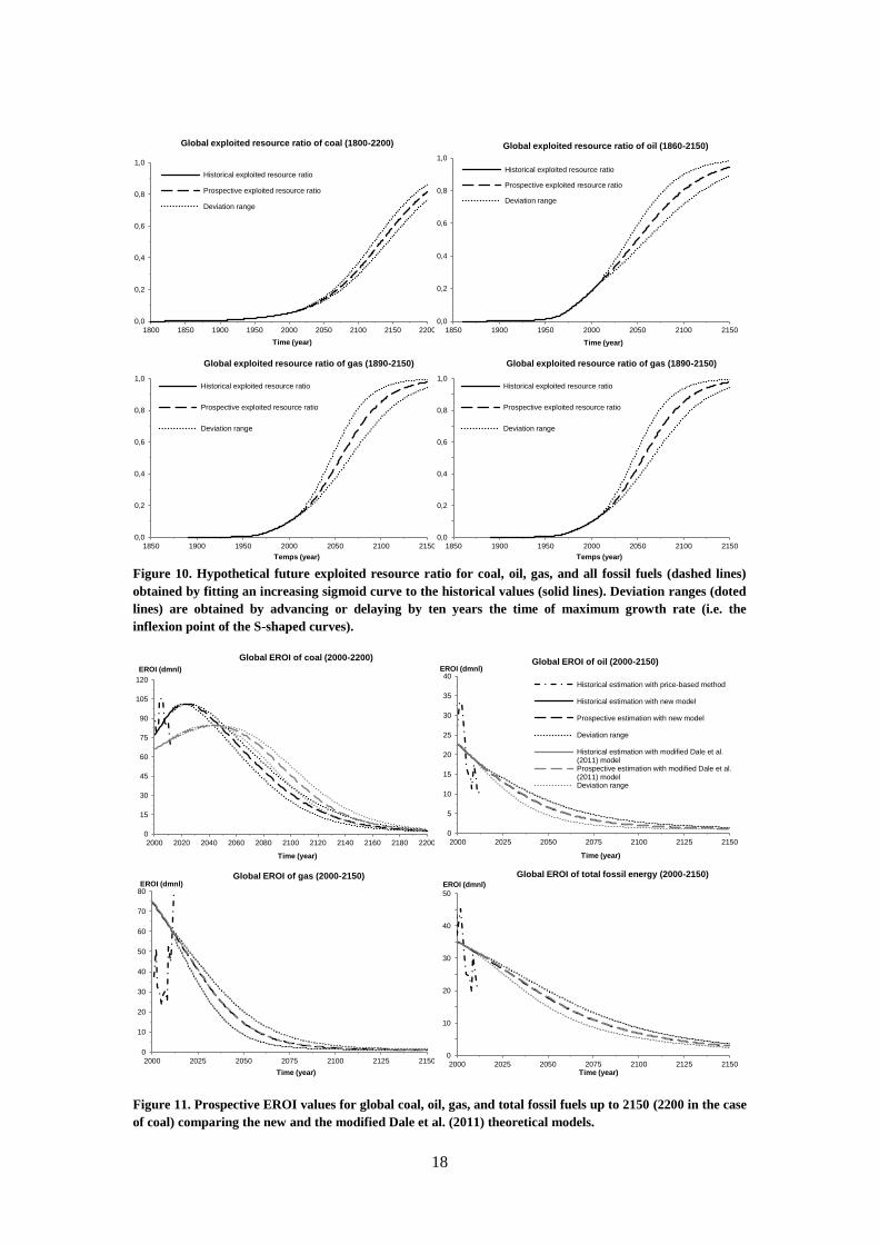
Figure 10. Hypothetical future exploited resource ratio for coal, oil, gas, and all fossil fuels (dashed lines)

obtained by fitting an increasing sigmoid curve to the historical values (solid lines). Deviation ranges (doted

lines) are obtained by advancing or delaying by ten years the time of maximum growth rate (i.e. the

inflexion point of the S-shaped curves).

Figure 11. Prospective EROI values for global coal, oil, gas, and total fossil fuels up to 2150 (2200 in the case

of coal) comparing the new and the modified Dale et al. (2011) theoretical models.

19

4. Discussion

4.1 Biases in the price-based approach

As can been seen in equation (6) and (7), our method to estimate the global EROI of

fossil fuels is logically sensitive to the uncertainty surrounding the value of its three

arguments, namely:

the prices of fossil energies presented in Figure 1,

the monetary-return-on-investment (MROI) supposed common to all scenarios but

varying over time thanks to (9),

the energy intensity (EI) taken as the global economy average and evolving over time

as shown in Figure 5.

The different fossil energy prices integrate investment in energy sectors but also different

kinds of rents, in particular during temporary exercise of market power. Those are not taken

into account in the MROI proxy. This implies that, on particular points that we cannot

identify, we might have overestimated the expenditures level in a given energy sector and

consequently underestimated its associated EROI. But considering that the fossil energy

prices come from historical data that we consider to be robust, we think that our results are

mostly subjected to the uncertainties surrounding the MROI and the EI.

Sensitivity of price-based results to the MROI

Regarding the estimates of the monetary-return-on-investment (MROI) in the energy

sector, we propose to test two variants of the one used so far that rest on the US long-term

interest rate. The three variants are labeled A, B, and C, with the following definition:

Variant A: the MROIA is based on the US long-term interest rate (US.LTIR)

presented in Figure 6, to which a risk premium of 10% is added following

Damodaran (2015).

Variant B: the MROIB is based on a reconstructed AMEX Oil Index11 based on a

relation estimated between the AMEX Oil Index of Reuters (2016) for the period

1984-2012 and the NYSE Index annual returns on this same period. NYSE Index

annual returns were retrieved from different references: Goetzmann et al. (2001) for

the 1815-1925 period, Ibbotson & Sinquefield (1976) for the 1926-1974 period, and

NYSE (2015) the 1975-2012 period (Figure 12).

Variant C: the MROIC is considered constant and equal to 1.1 (i.e. the energy sector

gross margin is 10%). This hypothesis is the one used in previous studies such as

King & Hall (2011), and King et al. (2015).

We summarize in Table 5 the different relations employed to estimate the MROI supposed

equal (for a given year) in all different fossil energy sectors.

11 The NYSE ARCA Oil Index, previously AMEX Oil Index, ticker symbol XOI, is a price-weighted index of the leading companies involved in the exploration, production, and development of petroleum. It measures the performance of the oil

industry through changes in the sum of the prices of component stocks. The index was developed with a base level of 125 as of

August 27th, 1984.

20

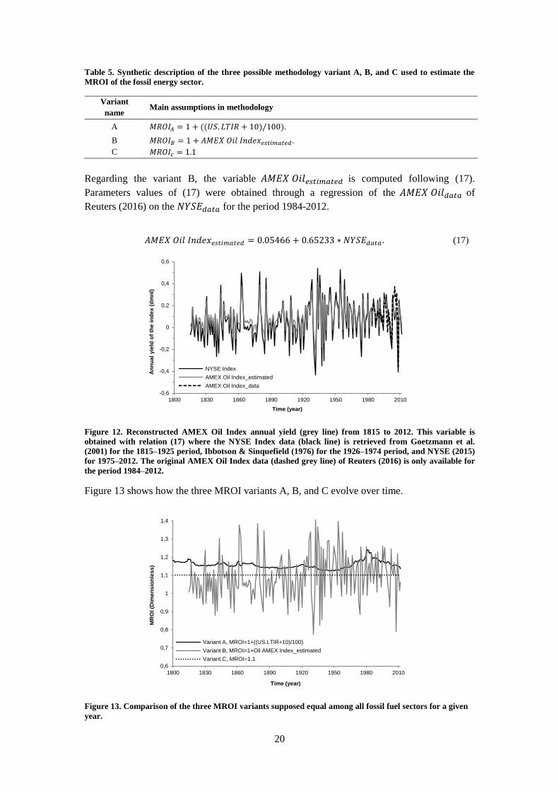
Table 5. Synthetic description of the three possible methodology variant A, B, and C used to estimate the

MROI of the fossil energy sector.

Variant

name Main assumptions in methodology

A 𝑀𝑅𝑂𝐼𝐴 = 1 + ((𝑈𝑆. 𝐿𝑇𝐼𝑅 + 10)/100).

B 𝑀𝑅𝑂𝐼𝐵 = 1 + 𝐴𝑀𝐸𝑋 𝑂𝑖𝑙 𝐼𝑛𝑑𝑒𝑥𝑒𝑠𝑡𝑖𝑚𝑎𝑡𝑒𝑑 .

C 𝑀𝑅𝑂𝐼𝑐 = 1.1

Regarding the variant B, the variable 𝐴𝑀𝐸𝑋 𝑂𝑖𝑙𝑒𝑠𝑡𝑖𝑚𝑎𝑡𝑒𝑑 is computed following (17).

Parameters values of (17) were obtained through a regression of the 𝐴𝑀𝐸𝑋 𝑂𝑖𝑙𝑑𝑎𝑡𝑎 of

Reuters (2016) on the 𝑁𝑌𝑆𝐸𝑑𝑎𝑡𝑎 for the period 1984-2012.

𝐴𝑀𝐸𝑋 𝑂𝑖𝑙 𝐼𝑛𝑑𝑒𝑥𝑒𝑠𝑡𝑖𝑚𝑎𝑡𝑒𝑑 = 0.05466 + 0.65233 ∗ 𝑁𝑌𝑆𝐸𝑑𝑎𝑡𝑎 . (17)

Figure 12. Reconstructed AMEX Oil Index annual yield (grey line) from 1815 to 2012. This variable is

obtained with relation (17) where the NYSE Index data (black line) is retrieved from Goetzmann et al.

(2001) for the 1815–1925 period, Ibbotson & Sinquefield (1976) for the 1926–1974 period, and NYSE (2015)

for 1975–2012. The original AMEX Oil Index data (dashed grey line) of Reuters (2016) is only available for

the period 1984–2012.

Figure 13 shows how the three MROI variants A, B, and C evolve over time.

Figure 13. Comparison of the three MROI variants supposed equal among all fossil fuel sectors for a given

year.

-0,6

-0,4

-0,2

0

0,2

0,4

0,6

1800 1830 1860 1890 1920 1950 1980 2010

An

nu

al

yie

ld o

f th

e i

nd

ex

(d

mn

l)

Time (year)

NYSE Index

AMEX Oil Index_estimated

AMEX Oil Index_data

0,6

0,7

0,8

0,9

1

1,1

1,2

1,3

1,4

1800 1830 1860 1890 1920 1950 1980 2010

MR

OI

(Dim

en

sio

nle

ss

)

Time (year)

Variant A, MROI=1+((US.LTIR+10)/100)

Variant B, MROI=1+Oil AMEX Index_estimated

Variant C, MROI=1.1

21

0

15

30

45

60

75

90

105

1800 1820 1840 1860 1880 1900 1920 1940 1960 1980 2000

EROI (dmnl)

Time (year)

Global EROI of coal (1800-2012)

Price-based variant A

Price-based variant B

Price-based variant C

0

10

20

30

40

50

60

70

80

1860 1875 1890 1905 1920 1935 1950 1965 1980 1995 2010

EROI (dmnl)

Time (year)

Global EROI of oil (1860-2012)

Price-based variant A

Price-based variant B

Price-based variant C

0

25

50

75

100

125

150

175

200

225

1890 1905 1920 1935 1950 1965 1980 1995 2010

EROI (dmnl)

Time (year)

Global EROI of gas (1890-2012)

Price-based variant A

Price-based variant B

Price-based variant C

0

10

20

30

40

50

60

70

1800 1820 1840 1860 1880 1900 1920 1940 1960 1980 2000

EROI (dmnl)

Time (year)

Global EROI of ftotal ossil energy (1800-2012)

Price-based variant A

Price-based variant B

Price-based variant C

Figure 14 presents our estimates of the global EROI of coal, oil, gas, and of the total primary

fossil energy system with the three possible MROI A, B, and C. It shows that our EROI

results are quite insensitive to the MROI variability. Indeed, the three MROI variants deliver

very consistent results. When looking at a particular energy type it is difficult to make a

distinction between the different EROI estimates because methodological alternatives do not

generates large enough output differences. This is particularly true for variant A and C which

are hardly discernible. However, it is worth noting that there is a slightly higher volatility in

values of variant B (that moreover cannot starts in 1800 because of the impossibility to

estimate the 𝑀𝑅𝑂𝐼𝐵 before 1815).

Figure 14. Comparison of variants A, B, and C, for estimating the global EROI of coal, oil, gas and total

fossil energy.

Sensitivity of price-based results to the energy intensity

It is very likely that the different expenditures of the global fossil energy sector

present overall a higher energy intensity than the average expenditures of the global economy.

Indeed, the share of energy-intensive capital components such as steel is higher in the energy

sector than in the global economy which relatively relies on more services (with less

embodied energy). Thus, by taking the energy intensity of the global economy as a proxy for

the energy intensity of the expenditures of the fossil energy sector, we should logically have

overestimated the different EROI that we have computed through our price-based

methodology. This choice was made in order to have a time-dependent energy intensity, and

Figure 5 shows that indeed the energy intensity of the global economy has substantially

decreased from 1800 (30 MJ/$1990) to 2012 (10 MJ/$1990). In their study concerning the

EROI of US oil and gas production, Guilford et al. (2011) also used a national average of the

energy intensity (8.3 MJ/$2005, i.e. 12.4 MJ/$1990), but they have then tested the sensitivity

of their results with two other values: an estimate of the energy intensity of the US oil & gas

industry expenditures of 14 MJ/$2005 (i.e. 20.92 MJ/$1990) based on the data of the Green

22

Design Institute of Carnegie-Mellon University, and an arbitrary high estimate of 20

MJ/$2005 (i.e. 29.9 MJ/$1990). In Figure 15 we show the effect of using energy intensities of

expenditures equal to 150% and 200% of the global economy average on our price-based

estimates of the global EROI of crude oil from 1860 to 2012. As previously anticipated, using

the global energy intensity average tends to imply an overestimation of the resulting EROI.

Nevertheless, the broad trend of the global EROI of crude oil is conserved and that is also true

for coal and gas, so we can be confident in our main results: maximum global EROI seems to

have been reached in the past for crude oil and gas, whereas increasing net energy yields are

still to come for coal global production.

Figure 15. Sensitivity of the global EROI of crude oil to the energy intensity, 1860–2012.

4.2 Comparison of price-based results with existing studies

To check the robustness of our price-based estimates we use the work of

Gagnon et al. (2009) in which an estimation of the global EROI of the combined oil and gas

production is presented from 1992 to 2006. Hence, using our price-based method, we built an

estimate of the global EROI of the joint oil and gas production (based on relative quantities of

production) and compared it to the one of Gagnon et al. (2009) in Figure 16. Overall, all our

estimates of the global EROI of oil and gas follows the same trend as the one of Gagnon et al.

(2009): an increase between 1992 and 1999 followed by a decreasing phase up to 2006. Our

estimation is globally higher and much more volatile than the one of Gagnon et al. (2009).

This difference mostly comes from the irreducible volatility of energy prices we used, and the

fact that we use a time-dependent energy intensity whereas in Gagnon et al. (2009) this

variable is constant and worth 20 MJ/$2005.

If we had computed the global EROI of combined oil and gas productions with an

energy intensity 150% higher than the global economy average, whatever the MROI variant,

results would have been much more in line with Gagnon et al. (2009). To estimate the

importance of the overall potential bias, we multiplied the denominator of the equation (7) by

a parameter that we calibrated in order to minimize the sum of squared errors deriving from

the difference between our estimation of the global EROI of oil and gas and the one of

Gagnon et al. (2009) on the period 1992-2006. We found that in average our EROIA

overestimate the one of Gagnon et al. (2009) by 20%. It is also worth noting that regarding

the EROI of coal, values around 80:1 presented by our results in the last decade are perfectly

in line with the estimation of the US coal EROI of Cleveland (2005).

0

15

30

45

60

75

90

1860 1880 1900 1920 1940 1960 1980 2000 2020

EROI (dmnl)

Time (year)

Global EROI of oil (1860-2012)

Energy Intensity= global average

Energy Intensity = 150% of global average

Energy Intensity = 200% of global average

23

Figure 16. Comparison of price-based global EROI of oil and gas with the one of Gagnon et al. (2009), 1992–

2006.

4.3 Sensitivity of EROI theoretical models to the URR

Given the potentially highly controversial aspect of the prospective results delivered by the

theoretical EROI models, sensitivity analysis needs be carried out. The key parameter of both

(“modified Dale et al., 2011” and “new”) theoretical EROI models is the value retained for

the URR. Let us first notice that, as can be seen in Figure 17 (up) for the case of coal, dividing

the URR by three by assuming an URR of 29 500 EJ (equaling the 1150 Gt best estimate

advanced by Mohr & Evans, 2009) instead of the previous 105 000 EJ hypothesis, does not

change the estimations of the past theoretical EROI from 1800 to 2012. This is because the

curve-fitting procedure (minimization of root square errors sum) generates a new set of

constant parameters for which the form of the past coal EROI trend remains consistent.

However, an URR of 29 500 EJ instead of 105 000 EJ generates a different historical

exploited resource ratio (Figure 17, down left) that has consequently a different prospective

evolution (still approached by a sigmoid increasing function). Finally (Figure 17, down right),

the combination of the alternative prospective exploited resource ratio and the new set of

constant parameters generate a different prospective EROI that reaches its maximum EROI

sooner, 2015 instead of 2023, and at a lower value, 93:1 instead of 101:1. Nevertheless,

considering that this sensitivity analysis has consisted in a three-fold division of the coal URR

estimation, these results can be considered as quite robust.

Furthermore, it is worth stating that if performed on the other two fossil fuels (oil and

gas), the sensitivity analysis consisting in a change of their respective URR only changes the

slope of their future respective decreasing EROI, but under no circumstances could it

generates a new EROI peak. This is mainly due to the fact that by definition in this study, oil

and gas comprise both conventional and unconventional fuels since estimations of historical

production of unconventional fuels are really scarce. Yet, given the increasing prevalence of

unconventional fossil fuels in the primary energy mix, it will be needed to perform again the

analyses of the present paper in a few decades. This could show that even if it is certain that

maximum EROIs have already been reached for conventional fossil fuels, it might not be the

case for their unconventional means of production. Indeed, the future preponderance of

unconventional fossil fuels production will enable a clear distinction between conventional

and unconventional fossil fuel EROIs, which will be of great interest since EROI gains in

unconventional production are expected by many whereas our results seems to indicate that

the time of increasing EROI has long past for conventional oil and gas production.

15

25

35

45

55

1992 1994 1996 1998 2000 2002 2004 2006

EROI (dmnl)

Time (year)

Pice-based variant A

Pice-based variant B

Pice-based variant C

Gagnon et al., 2009

24

-10

5

20

35

50

65

80

95

110

1800 1820 1840 1860 1880 1900 1920 1940 1960 1980 2000 2020

EROI (dmnl)

Time (year)

Global EROI of coal (1800-2012)

Historical estimation with price-based method

Historical estimation with new model (URR=105 000 EJ)

Historical estimation with new model (URR=29 500 EJ)

0,0

0,2

0,4

0,6

0,8

1,0

1800 1850 1900 1950 2000 2050 2100 2150

Time (year)

Global exploited resource ratio of coal (1800-2150)

Historical exploited resource ratio(URR=105 000 EJ)

Prospective exploited resource rato(URR=105 000 EJ)

Deviation range (URR=105 000 EJ)

Historical exploited resource ratio(URR=29 500 EJ)

Prospective exploited resource rato(URR=29 500 EJ)

Deviation range (URR=29 500 EJ)0

20

40

60

80

100

120

2000 2020 2040 2060 2080 2100 2120 2140

EROI (dmnl)

Time (Years)

Global EROI of coal (2000-2150)

Historical estimation with price-based methodHistorical estimation with new model (URR=105 000 EJ)Prospective estimation with new model (URR= 105 000 EJ)Deviation range (URR=105 000 EJ)Historical estimation with new model (URR=29 500 EJ)Prospective estimation with new model (URR= 29 500 EJ)Deviation range (URR=29 500 EJ)

Figure 17. Sensitivity analysis of the “new” theoretical EROI model in the case of coal, using the 29 500 EJ

URR estimation of Mohr & Evans (2009) instead of the 105 000 EJ estimate of McGlade & Ekins (2015).

5. Conclusion and perspectives

So far historical EROI trends had been estimated for a few decades at most.

Consequently, the hypothesis that maximum EROI of fossil fuels had already been reached

long ago had been advanced several times without any real verification. In order to address

this problem we have first relied on a price-based approach. By collecting and harmonizing

several types of data, we have provided a very long term historical perspective of (constant

$1990) fossil energy prices per same energy unit (TJ)12. This has allowed us to estimate the

quantity-weighted average price of aggregated fossil energy from 1800 to 2012. Then, thanks

to three variant MROI estimates that proved to deliver very consistent results, we have

estimated the global EROI of coal, oil, and gas from the beginning of their production (1800,

1860, and 1890 respectively) to 2012, which furthermore allowed us to compute an EROI for

the global primary fossil energy sector from 1800 to 2012. The results of this methodology

have proved to be consistent with the existing historical estimation of global oil and gas

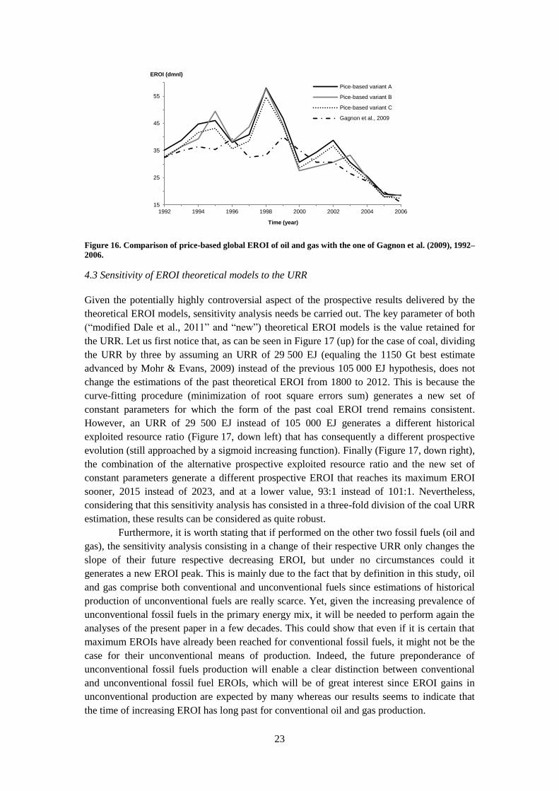
production of Gagnon et al. (2009) made from 1992 to 2006. Good consistency with

Cleveland (2005) was also found for what could be considered as the current (i.e. beginning

of twentieth century) EROI of coal. Our price-based estimates of global historical fossil fuels

EROIs have shown that maximum EROIs were reached in the 1930s–40s for oil and gas,

respectively around 50:1 and 150:1, whereas the maximum EROI of global coal is still to

12 The tremendous work of Fouquet (2008) offers an even more precise historical perspective on energy prices with however a

geographical perimeter restricted to the UK and a focus on energy services and not primary energy.

25

come. We have then confirmed these historical price-based EROI estimates with a

comparison to a theoretical expression of the EROI of a given energy resource as a function

of its cumulated production. In order to do that, we have first show that the theoretical model

originally developed by Dale et al. (2011) needed some amendments to comply with physical

reality. Of course, the two theoretical models that we have tested gave much more smoothed

trends compared to the price-based method, but overall we observe a good concordance

between the two approaches and, as already said, with more empirical analyses such as

Gagnon et al. (2009) and Cleveland (2005). This comparison indicates that “real” physical

past EROIs are somewhere between the extra-smooth estimate of theoretical models and the

more volatile price-based estimations. The EROI theoretical models also allowed us to

perform some prospective estimates of future fossil fuels EROI. This work is especially

interesting regarding coal since its maximum EROI has not yet been reached. Simulations

have showed discrepancies among models and URR hypotheses that logically prevent any

attempt to determine with assurance the time and the value of the future coal EROI peak.

However, considering the several models we have used, and the two very different URR

estimations that we have tested, it can be fairly postulated that the maximum coal EROI will

occur between 2020 and 2045, around a value of around 95(±15):1.

This study also promotes new avenues for future researches. Indeed, since biomass

energy has occupied a central role in the past of industrial economies, and still represents the

largest part of the renewable energy supply at global level by providing an important share of

the energy supply of developing countries, estimating the historical EROI of biomass energy

should be a research priority. This would allow estimating the global historical EROI of the

whole economy from 1800 (or even before) to present times. Unfortunately, since global

biomass energy is primarily used in non-commercial channels that are disconnected from

markets and their associated prices, another methodology than the one presented in this paper

would have to be used. Moreover, our study has focused on primary energy but regarding the

fact that electricity ensures a growing share of global final energy consumption, we think that

future researches should also focus on estimating long-term trends in final and not primary

EROI. Finally, as we have based our work only a global view of the economy, we think it

should be really interesting to replicate this work at a national level, in particular in

developing countries which are likely to be more sensitive to energy prices.

Acknowledgements

The authors would like to thank Pierre-André Jouvet, Frédéric Lantz, and Nicolas

Legrand for their helpful comments on an earlier version of this article. Two anonymous

reviewers have added much to the quality of this article thanks to their insightful

comments.

References

Ayres, R.U., 1998. Eco-thermodynamics: economics and the second law. Ecological

Economics, 26, pp.189–209.

Ayres, R.U. & Warr, B., 2009. The Economic Growth Engine: How Energy and Work Drive

Material Prosperity, Cheltenham, UK: Edward Elgar Publishing.

British Petroleum, 2015. Statistical Review of World Energy 2015, Available at:

http://www.bp.com/en/global/corporate/energy-economics/statistical-review-of-world-

energy.html.

26

Cleveland, C., 2005. Net energy from the extraction of oil and gas in the United States.

Energy, 30, pp.769–782.

Cleveland, C.J. et al., 1984. Energy and the U.S. economy: a biophysical perspective. Science,

225(4665), pp.890–897.

Court, V., Jouvet, P.-A. & Lantz, F., 2017. Long-term endogenous economic growth and

energy transitions. The Energy Journal, (forthcoming).

Dale, M., Krumdieck, S. & Bodger, P., 2011. A Dynamic Function for Energy Return on

Investment. Sustainability, 3, pp.1972–1985.

Dale, M., Krumdieck, S. & Bodger, P., 2012. Global energy modelling — A biophysical

approach ( GEMBA ) Part 2 : Methodology. Ecological Economics, 73, pp.158–167.

Damodaran, A., 2015. Total Beta by Industry Sector. Risk/Discount Rate. Available at:

http://pages.stern.nyu.edu/~adamodar/.

Etemad, B. & Luciani, J., 1991. World Energy Production, 1800-1985. Production Mondiale

d’Énergie, 1800-1985, Geneve, CH: Librairie Droz.

Faber, M., Niemes, H. & Stephan, G., 1987. Entropy, Environment and Resources: An Essay

in Physio-economics, Berlin, DE: Springer.

Fernandes, S.D. et al., 2007. Global Biofuel Use, 1850-2000. Global Biogeochemical Cycles,

21(2), pp.1–15.

Fizaine, F. & Court, V., 2015. Renewable Electricity Producing Technologies and Metal

Depletion: A Sensitivity Analysis Using the EROI. Ecological Economics, 110, pp.106–

118.

Fouquet, R., 2008. Heat, Power and Light: Revolutions in Energy Services, Northampton,

MA: Edward Elgar Publishing.

Gagnon, N., Hall, C.A.S. & Brinker, L., 2009. A preliminary investigation of energy return on

energy investment for global oil and gas production. Energies, 2(3), pp.490–503.

Georgescu-Roegen, N., 1979. Energy Analysis and Economic Valuation. Southern Economic

Journal, 45(4), pp.1023–1058.

Georgescu-Roegen, N., 1971. The Entropy Law and the Economic Process., Cambridge, MA:

Harvard University Press.

Goetzmann, W.N., Ibbotson, R.G. & Peng, L., 2001. A new historical database for the NYSE

1815 to 1925: Performance and predictability. Journal of Financial Markets, 4(1), pp.1–

32.

Guilford, M.C. et al., 2011. A new long term assessment of energy return on investment

(EROI) for U.S. oil and gas discovery and production. Sustainability, 3(10), pp.1866–

1887.

Hall, C.A.S. et al., 2001. The need to reintegrate the natural sciences with economics.

BioScience, 51(8), p.663–673.

Hall, C.A.S., Balogh, S. & Murphy, D.J.R., 2009. What is the Minimum EROI that a

Sustainable Society Must Have? Energies, 2(1), pp.25–47.

Hall, C.A.S. & Day, J.W., 2009. Revisiting the Limits to Growth After Peak Oil. American

Scientist, 97(3), p.230.

Hall, C.A.S. & Klitgaard, K.A., 2012. Energy and the Wealth of Nations: Understanding the

Biophysical Economy, New York, NY: Springer.

Hall, C.A.S. & Klitgaard, K.A., 2006. The need for a new, biophysical-based paradigm in

economics for the second half of the age of oil. International Journal of

Transdisciplinary Research, 1(1), pp.4–22.

Hall, C.A.S., Lambert, J.G. & Balogh, S.B., 2014. EROI of different fuels and the

implications for society. Energy Policy, 64, pp.141–152.

27

Hubbert, K., 1956. Nuclear Energy and the Fossil Fuels, San Antonio, Texas.

Ibbotson, R.G. & Sinquefield, R.A., 1976. Stocks, Bonds, Bills, and Inflation: Year-by-Year

Historical Returns (1926-1974). The Journal of Business, 49(1), pp.11–47.

IIASA, 2012. Global Energy Assessment - Toward a Sustainable Future, Vienna, AT.

King, C., Maxwell, J. & Donovan, A., 2015. Comparing World Economic and Net Energy

Metrics, Part 1: Single Technology and Commodity Perspective. Energies, 8(12),

pp.12949–12974.

King, C.W. & Hall, C.A.S., 2011. Relating Financial and Energy Return on Investment.

Sustainability, 3(10), pp.1810–1832.

Krysiak, F.C., 2006. Entropy, limits to growth, and the prospects for weak sustainability. , 58,

pp.182–191.

Kummel, R., 2011. The Second Law of Economics: Energy, Entropy, and the Origins of

Wealth, New York, NY: Springer.

Lambert, J.G. et al., 2014. Energy, EROI and quality of life. Energy Policy, 64, pp.153–167.

Maddison, A., 2007. Contours of the World Economy, 1− 2030 AD: Essays in Macro-

Economic History, Oxford, UK: Oxford University Press.

Manthy, R.S., 1978. Natural Resource Commodities - A Century of Statistics, Washington,

DC: John Hopkins Press for Resources for the Future.

McGlade, C. & Ekins, P., 2015. The geographical distribution of fossil fuels unused when

limiting global warming to 2 °C. Nature, 517, pp.187–190.

Mohr, S.H. & Evans, G.M., 2009. Forecasting coal production until 2100. Fuel, 88(11),

pp.2059–2067.

Murphy, D.J. et al., 2011. Order from Chaos: A Preliminary Protocol for Determining the

EROI of Fuels. Sustainability, 3(10), pp.1888–1907.

Murphy, D.J. & Hall, C.A.S., 2011a. Adjusting the economy to the new energy realities of the

second half of the age of oil. Ecological Modelling, 223(1), pp.67–71.

Murphy, D.J. & Hall, C.A.S., 2011b. Energy return on investment, peak oil, and the end of

economic growth. Annals of the New York Academy of Sciences, 1219(1), pp.52–72.

Murphy, D.J. & Hall, C.A.S., 2010. Year in review-EROI or energy return on (energy)

invested. Annals of the New York Academy of Sciences, 1185(1), pp.102–118.

NYSE, 2015. NYSE Composite Index: Annual Returns. Available at: http://www.forecast-

chart.com/historical-nyse-composite.html.

O’Connor, M., 1991. Entropy, structure, and organisational change. Ecological Economics, 3,

pp.95–122.

Odum, H.T., 1973. Energy, Ecology, and Economics. AMBIO, 2(6), pp.220–227.

Odum, H.T., 1971. Environment, Power, and Society, New York, NY: Wiley-Interscience.

Officer, L. & Williamson, S., 2016. The Annual Consumer Price Index for the United States,

1774-2015. MeasuringWorth.com. Available at:

http://www.measuringworth.com/uscpi/.

Officer, L.H., 2016. What Was the Interest Rate Then? MeasuringWorth.com. Available at:

http://www.measuringworth.com/interestrates/.

Perrings, C., 1987. Economy and Environment: A Theoretical Essay on the Interdependence

of Economic and Environmental Systems, Cambridge, UK: Cambridge University Press.

Reuters, 2016. Amex Oil Index. Available at:

http://www.reuters.com/finance/markets/index?symbol=.XOI.

Rühl, C. et al., 2012. Economic development and the demand for energy: A historical

perspective on the next 20 years. Energy Policy, 50, pp.109–116.

Smil, V., 2005. Creating the Twentieth Century: Technical Innovations of 1867-1914 and

28

Their Lasting Impact, New York, NY: Oxford University Press.

Smil, V., 2010. Energy Transitions: History, Requirements, Prospects, Santa Barbara, CA:

Praeger Publishers Inc.

Sorrell, S. et al., 2010. Global oil depletion: a review of the evidence. Energy Policy, 38(9),

pp.5290–5295.

The Maddison Project, 2013. GDP per Capita 1-2010 AD. Available at:

http://www.ggdc.net/maddison/maddison-project/home.htm.

The Shift Project, 2015. Historical Energy Production Statistics. Available at: http://www.tsp-

data-portal.org/Energy-Production-Statistics#tspQvChart.

United Nations, 2015. Department of Economic and Social Affairs, Population Division,

World Population Prospects, the 2015 Revision. Available at:

http://esa.un.org/unpd/wpp/Download/Standard/Population/.

US Bureau of the Census, 1975. Historical Statistics of the United States, Colonial Times to

1970. Bicentennial Edition, Part 1, Washington, DC. Available at:

https://fraser.stlouisfed.org/docs/publications/histstatus/hstat1970_cen_1975_v1.pdf.

US Energy Information Administration (EIA), 2013. Annual Coal Report 2012, Available at:

http://www.eia.gov/coal/annual/archive/05842012.pdf.

US Energy Information Administration (EIA), 2012. Annual Energy Review 2011, Available

at: https://www.eia.gov/totalenergy/data/annual/pdf/aer.pdf.

US Energy Information Administration (EIA), 2014. International Energy Statistics database.

Available at: http://www.eia.gov/cfapps/ipdbproject/IE.

US Energy Information Administration (EIA), 2016. Monthly Energy Review (June 2016),

Available at: http://www.eia.gov/totalenergy/data/monthly/pdf/mer.pdf.

World Bank, 2016. World Bank Indicators, GDP growth (annual %). Available at:

http://data.worldbank.org/indicator/NY.GDP.MKTP.KD.ZG.