39
Longitudinal Data Analysis for Social Science Researchers Re-introducing Analysis Methods www.longitudinal.stir.ac.uk
| Date post: | 14-Dec-2015 |
| Category: |
Documents |
| Upload: | stanley-riley |
| View: | 218 times |
| Download: | 0 times |
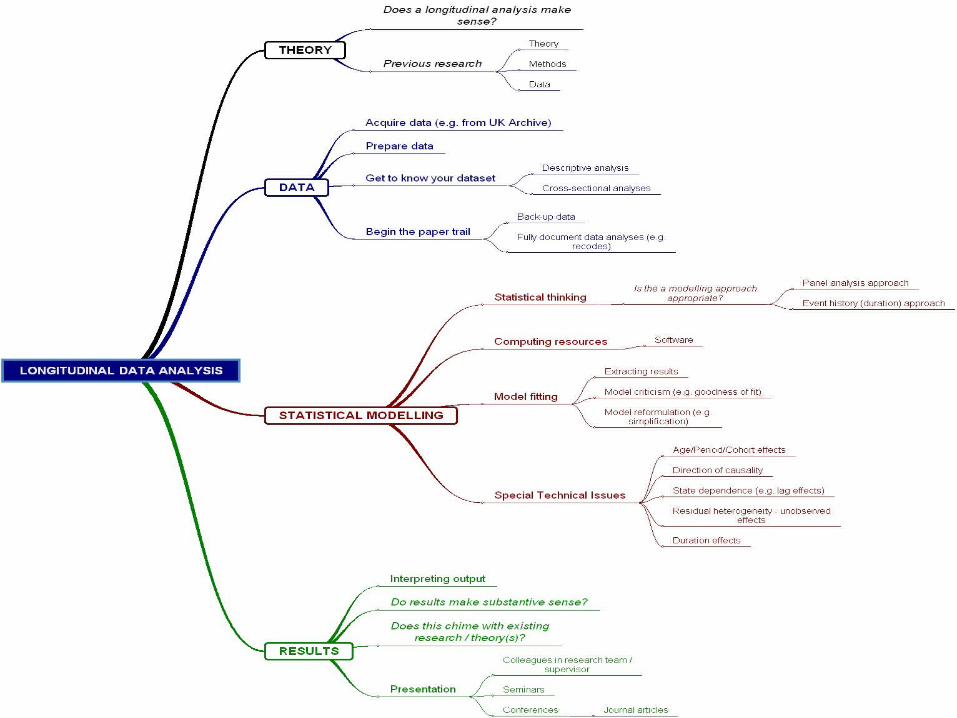
Longitudinal Data Analysis for Social Science Researchers
Re-introducing Analysis Methods
www.longitudinal.stir.ac.uk
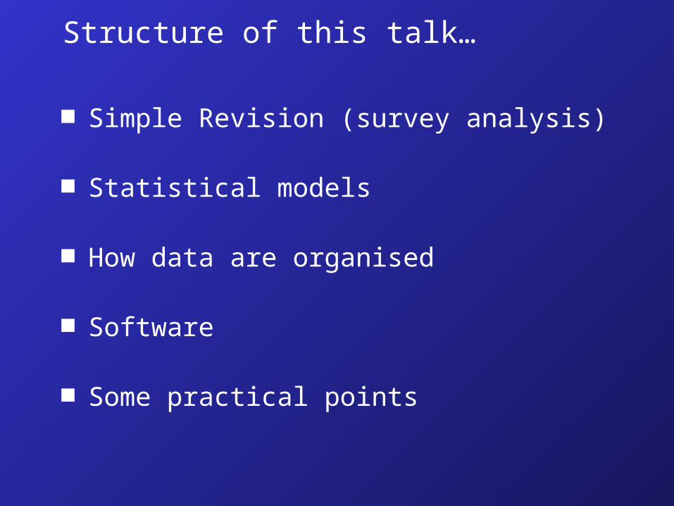
Structure of this talk…
Simple Revision (survey analysis)
Statistical models
How data are organised
Software
Some practical points

Notation and terms -
Notation and terms are never completely standard but we’ll try to keep things consistent

A Joke…

1,...,3;)'exp(1
)'exp(=j
x
x
it
it
j
j

These equations are all Greek to me!

Simple Revision
Probability p Odds (p/1-p) Probability therefore = (odds/1+odds) Logarithm denoted as ln The anti-log or exponential is denoted
as exp Greek symbol is the sum of
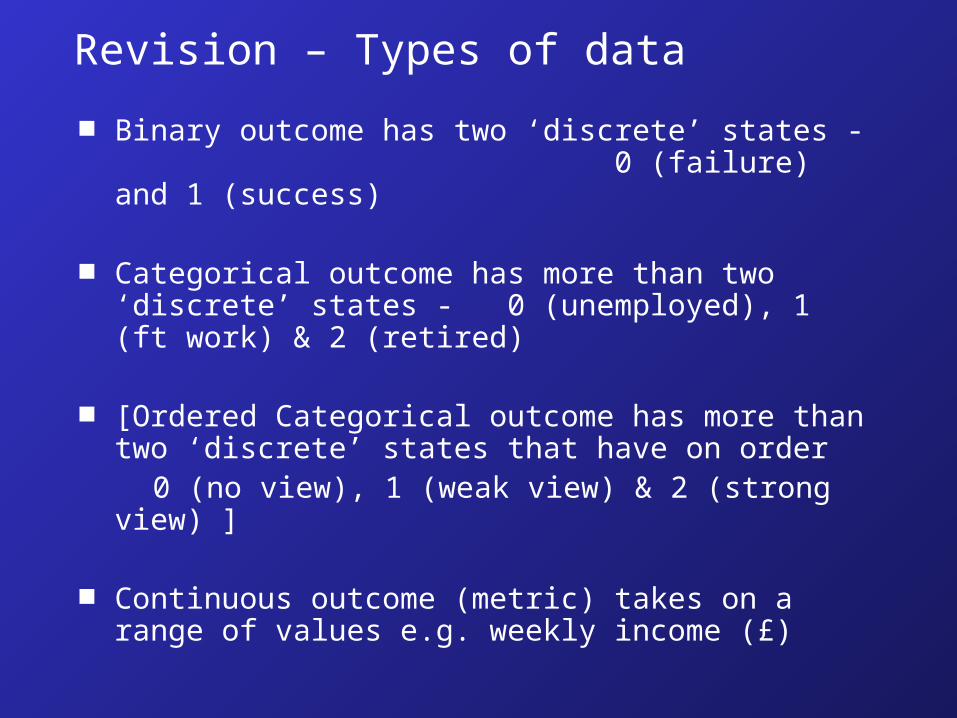
Revision – Types of data
Binary outcome has two ‘discrete’ states - 0 (failure) and 1 (success)
Categorical outcome has more than two ‘discrete’ states - 0 (unemployed), 1 (ft work) & 2 (retired)
[Ordered Categorical outcome has more than two ‘discrete’ states that have on order
0 (no view), 1 (weak view) & 2 (strong view) ]
Continuous outcome (metric) takes on a range of values e.g. weekly income (£)

Statistical Models

Why model data?
My view – It might be controversial…. In social science research it is unlikely that a bivariate (two variable) explanation will capture the complexity of the real social world. Therefore there is no choice other than to fit a statistical model.
In social science research, unlike in experimental situations, ‘randomisation’ is very often not appropriate. Therefore there is a lack of control and a need for more advanced statistical methods.

In simple terms a model does two things…
Tells us what is important (e.g. which variables are significant).
Tell us how important variables are (i.e. their strength).
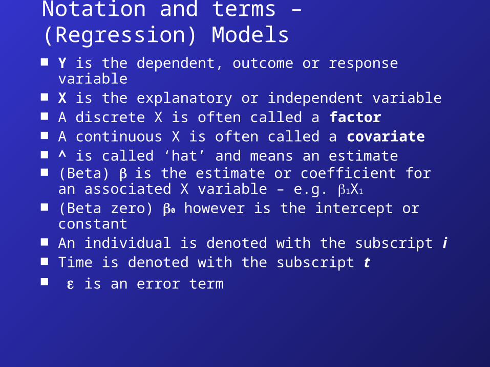
Notation and terms – (Regression) Models Y is the dependent, outcome or response
variable X is the explanatory or independent variable A discrete X is often called a factor A continuous X is often called a covariate ^ is called ‘hat’ and means an estimate (Beta) is the estimate or coefficient for an
associated X variable – e.g. 1X1
(Beta zero) 0 however is the intercept or constant
An individual is denoted with the subscript i Time is denoted with the subscript t is an error term
How data are organised

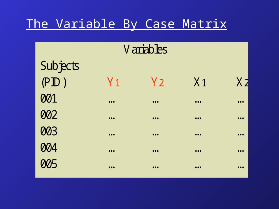
The Variable By Case Matrix Variables Subjects (PID) Y1 X1 X2 X3 001 … … … … 002 … … … … 003 … … … … 004 … … … … 005 … … … …

The Variable By Case Matrix Variables Subjects (PID) Y1 X1 X2 X3 001 … … … … 002 … … … … 003 … … … … 004 … … … … 005 … … … …
The variable by case matrix – with a measure of Y at a certain time point
The Variable By Case Matrix
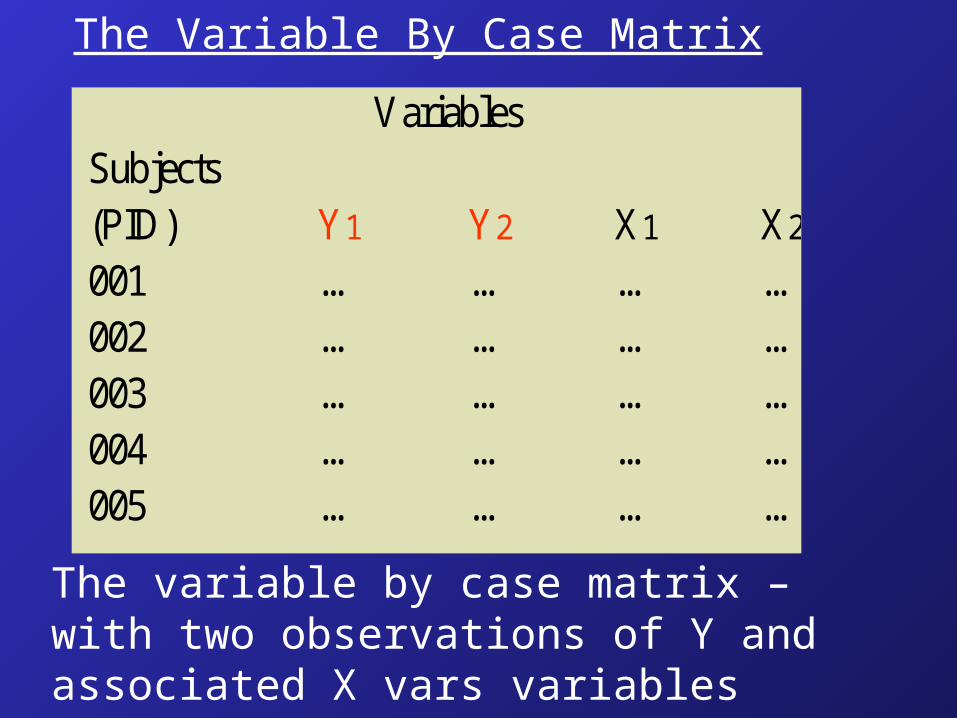
Variables Subjects (PID) Y1 Y2 X1 X2 001 … … … … 002 … … … … 003 … … … … 004 … … … … 005 … … … …
The Variable By Case Matrix
Variables Subjects (PID) Y1 Y2 X1 X2 001 … … … … 002 … … … … 003 … … … … 004 … … … … 005 … … … …
The variable by case matrix – with two observations of Y and associated X vars variables
This is sometimes called wide format e.g. in STATA.
Example: BHPS teaching datasets
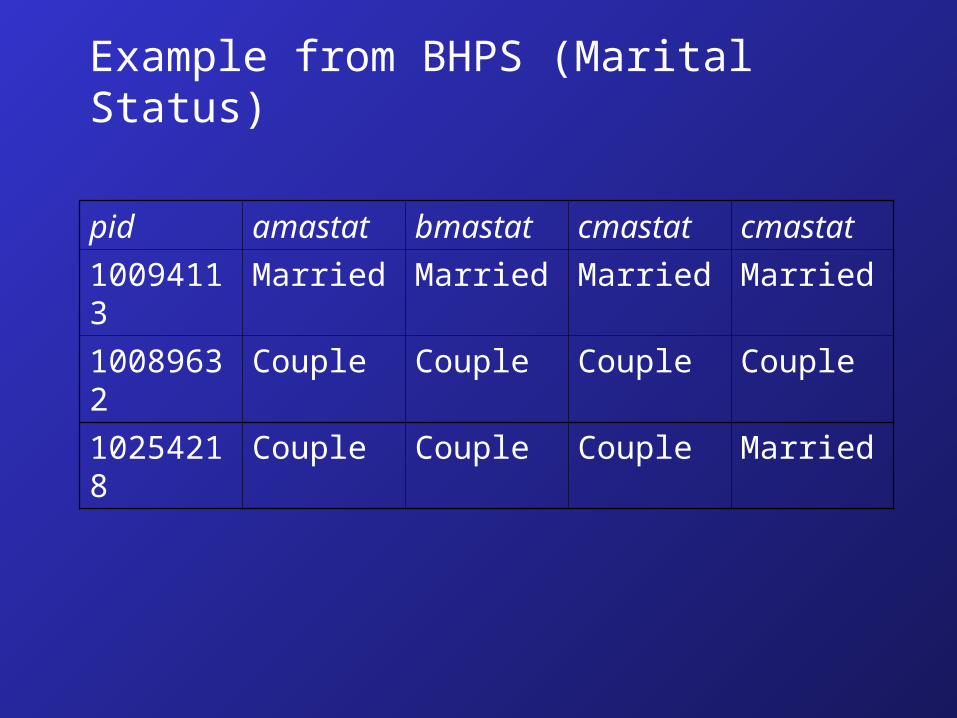
Example from BHPS (Marital Status)
pid amastat bmastat cmastat cmastat
10094113
Married Married Married Married
10089632
Couple Couple Couple Couple
10254218
Couple Couple Couple Married
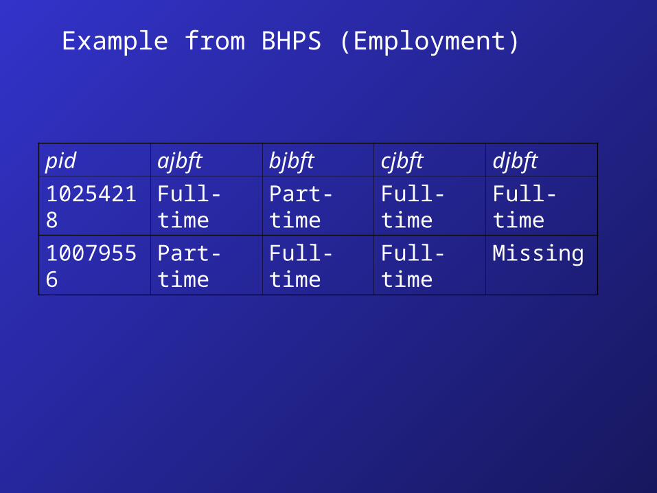
Example from BHPS (Employment)
pid ajbft bjbft cjbft djbft
10254218
Full-time Part-time
Full-time Full-time
10079556
Part-time
Full-time Full-time Missing

The Variable By Case Matrix
Variables Subjects Y1t X1t X2 t X3 t 001 … … … … 001 … … … … 002 … … … … 002 … … … …

The Variable By Case Matrix
Variables Subjects Y1t X1t X2 t X3 t 001 … … … … 001 … … … … 002 … … … … 002 … … … …
The variable by case matrix – with two observations of Y and associated X variables

The variable by case matrix – with two observations of Y and associated X variables
This is sometimes called long format e.g. in STATA.
Note: This is the usual format for undertaking longitudinal data analysis.The BHPS and other surveys usually require data management to construct a long format file.

Example from BHPS
pid zage zmastat wave12287407 67 married 212287407 68 married 312287407 69 married 412287407 70 married 512287407 71 married 612287407 72 married 712287407 73 married 812287407 74 married 912287407 75 married 1012287407 76 married 1112287407 77 married 12

Software
Our overall message is that if you are serious about doing longitudinal analyses try to move to using STATA as soon as possible!

STATA Version 9.1 www.stata.com
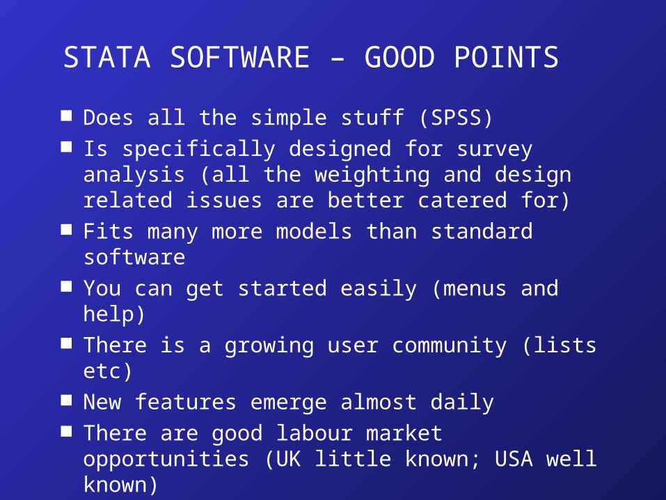
STATA SOFTWARE – GOOD POINTS
Does all the simple stuff (SPSS) Is specifically designed for survey analysis
(all the weighting and design related issues are better catered for)
Fits many more models than standard software
You can get started easily (menus and help) There is a growing user community (lists
etc) New features emerge almost daily There are good labour market opportunities
(UK little known; USA well known)
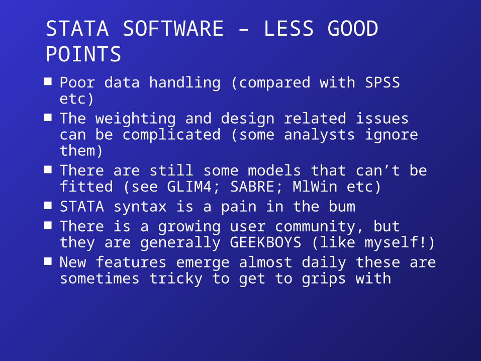
STATA SOFTWARE – LESS GOOD POINTS Poor data handling (compared with SPSS etc) The weighting and design related issues can
be complicated (some analysts ignore them) There are still some models that can’t be
fitted (see GLIM4; SABRE; MlWin etc) STATA syntax is a pain in the bum There is a growing user community, but they
are generally GEEKBOYS (like myself!) New features emerge almost daily these are
sometimes tricky to get to grips with
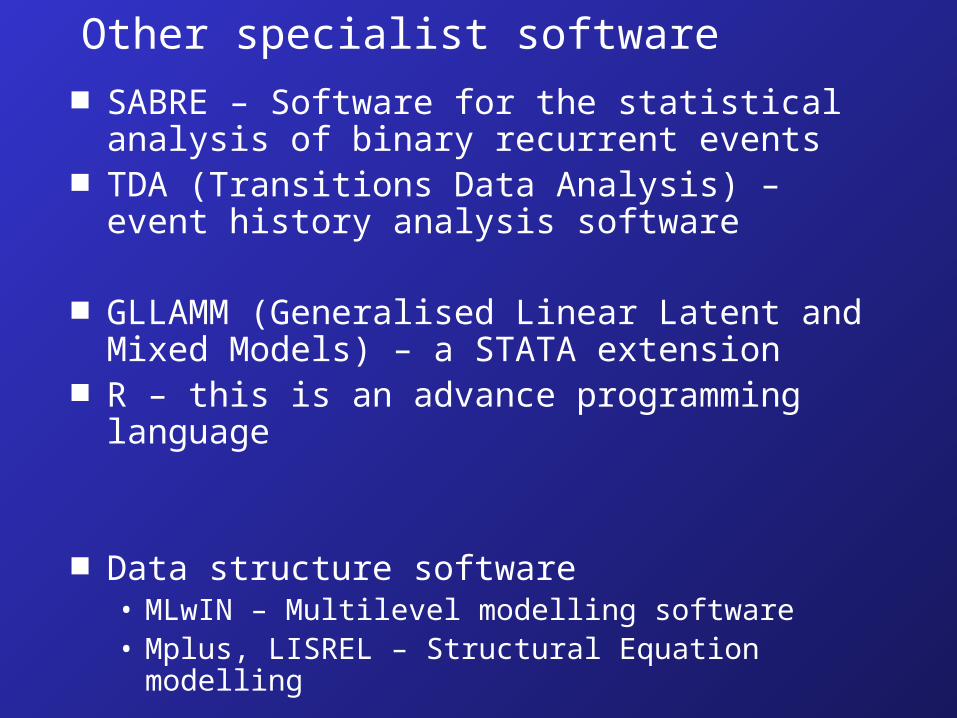
Other specialist software SABRE – Software for the statistical
analysis of binary recurrent events TDA (Transitions Data Analysis) – event
history analysis software
GLLAMM (Generalised Linear Latent and Mixed Models) – a STATA extension
R – this is an advance programming language
Data structure software• MLwIN – Multilevel modelling software• Mplus, LISREL – Structural Equation
modelling

Some Practical Thoughts…
“The best habit you can get into is to get into good habits”
..See handout: Statistical modelling – some notes and reflections

STATISTICAL MODELLING –SOME NOTES AND REFLECTIONS (Most of which will be ludicrously familiar)

The Paper Trail
Ensure that all serious work can be reproduced i.e. have a clear ‘paper trail’ in place.
The platinum standard is that if a research assistant/fellow was killed in a freak accident the professor could complete the project.
The gold standard is that all files and notes are correctly and clearly set out so that they can be passed on to someone without much explanation. This will mean that you and the other members of the research team can follow the paper trail and therefore subsequently reproduce and augment material if required. This is particularly important as referees can often ask for minor, and in the case of some of my work major, amendments to statistical analysis.

Working with syntax will tend to help you in these aims.
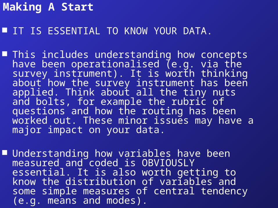
Making A Start
IT IS ESSENTIAL TO KNOW YOUR DATA.
This includes understanding how concepts have been operationalised (e.g. via the survey instrument). It is worth thinking about how the survey instrument has been applied. Think about all the tiny nuts and bolts, for example the rubric of questions and how the routing has been worked out. These minor issues may have a major impact on your data.
Understanding how variables have been measured and coded is OBVIOUSLY essential. It is also worth getting to know the distribution of variables and some simple measures of central tendency (e.g. means and modes).

Making A Start
Make sure that you are working with the best data available. In the case of the BHPS this will be the most recent release of the data.
ALWAYS MAKE BACK-UP FILES. Work with as clean a set of data as possible.
Always start with exploratory analysis.
EVERY recode, compute, re-labelling task should be documented and be traceable in the paper trail.
DON’T START MODELLING TOO SOON!
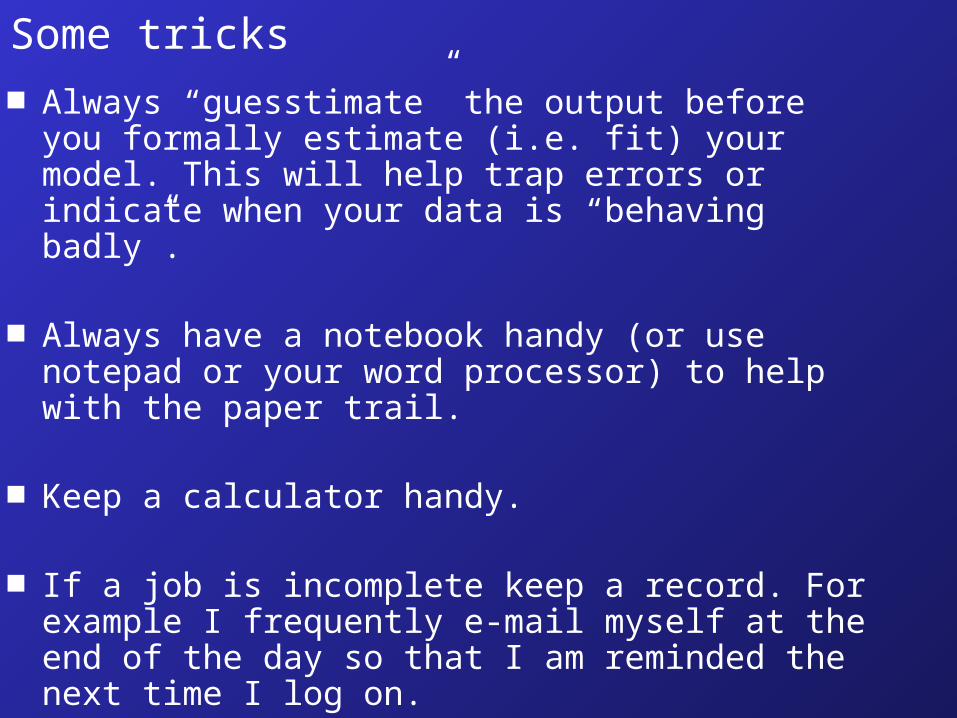
Some tricks Always “guesstimate” the output before you
formally estimate (i.e. fit) your model. This will help trap errors or indicate when your data is “behaving badly”.
Always have a notebook handy (or use notepad or your word processor) to help with the paper trail.
Keep a calculator handy.
If a job is incomplete keep a record. For example I frequently e-mail myself at the end of the day so that I am reminded the next time I log on.

Statistical modelling
Always proceed from a position informed by substantive theory. The economists are particularly good at this (although occasionally a little rigid). The modelling building process should (ideally) always be guided at all stages by your substantive theory(s).

Statistical modelling
REMEMBER – REAL DATA IS MUCH MORE MESSY, BADLY BEHAVED, HARD TO INTERPRET ETC. THAN THE DATA USED IN BOOKS AND AT WORKSHOPS.
In the case of longitudinal analysis spend as much time as possible getting the underlying social process clear before you fit a model. The best way to do this is to build upon well thought out cross-sectional analysis.