37
Longitudinal Network Analysis
| Date post: | 01-Jan-2016 |
| Category: |
Documents |
| Upload: | kellie-estes |
| View: | 35 times |
| Download: | 3 times |

Longitudinal Network Analysis
Content
• Basic model assumptions in SIENA
• Exercise
• Interpretation of results
• Improvement of model
• Further relevant topics
Basic model assumptions in SIENA
What are the assumptions SIENA makes and can you apply SIENA to test your
hypotheses?

Let‘s start with a small movie……
• Communication in a class room with two teachers
• All communication was observed.

Model assumptions 1 / 2
• Most observed networks in social sciences are censored data. They desribe the current state of a network but this state is the outcome of unobserved processes and subject to further change
– Plausible for many networks: friendship, trust, exchange.
– Plausible for your network?
• Networks change in micro steps. Micro steps of actors in the network account for large changes in the observed networks (t1, t2, t3, ….. tn).
• Markov process: For any point in time, the current state of the network determines probabilistically its further evolution, and there are no additional effects of the earlier past. All relevant information is therefore assumed to be included in the current state.
– Social network change as endogeneous process: social network is the social context that influences the probabilties of ist own change
– But: one can include exogeneous effects: constant covariates or changing covariates

Model assumptions 2 / 2
• Actors control their outgoing ties = Actor-based model: Actors change their outgoing ties on basis of their and others‘ attributes, their position in the network, and their perceptions about the rest of the network
– This is more plausible for directed graphs. In undirected graphs one actor will take the iniatiative.
– Options for actors are to create a tie, withdraw a tie, or do nothing
– Theoretical problem of limited information: Can you justify that actors are aware of others‘ attributes or even the wider network (e.g., actors at distance two)?
• Bringing the individual back in (Kilduff & Krackhardt, 1994).
• Structural individualism (Udehn, 2002; Hedström, 2005)
• No more than one tie can change at a time:
– Sequential change. Denies the possibility of coordinated action.
The stochastic estimation processes
1. Estimation of frequency of opportunities a actor can make to change a tie (not doing anything is also a choice an actor can make)
– How many micro steps does the model require to arrive at the observed network?
2. Estimation of user-specified effects on the probabilities of tie change
– E.g., Does and actor‘s attribute or the tendency to reciprocate contribute to explain the observed model?
– Parameter estimates are based on a simulation that uses t1 as starting point to predict the subsequent observed network -> conditional method of moments estimation.
– t1 is not modeled but only used as input.
3. The estimation process takes time! Depending on your network size and the amount of parameters it can take several hours to run one estimation.
– Use fast computers
– Use multiple computers
– Define your models well
Defining a model
• Check if the basic assumptions of SIENA are in agreement with your model!!! If not, try to use another mehtod. Social network analysis is (should be) theory driven not driven by the method!
• The objective function is the part of SIENA that allows you to define how you expect actors form ties in a network
– It is the rule of network behavior we assume in our theory
– Like in linear statistical models the probability to change a tie is the linear combination of effects specified by the user accoding to a theoretical model
– If a effect is estimated to be positive an actor will make a choice that leads to a network state where the corresponding effect is higher. The converse applies when the effect is negative. If the parameter is estimated to be zero, the effect is irrelevant for actors‘ choices.
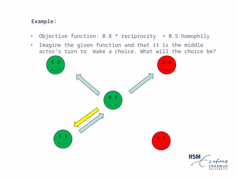
Example:
• Objective function: 0.8 * reciprocity + 0.5 homophily
• Imagine the given function and that it is the middle actor‘s turn to make a choice. What will the choice be?

Time for an example:
• Objective function: 0.8 * reciprocity + (- 0.5 )homophily
• Imagine the given function and that it is the middle actor‘s turn to make a choice. What will the choice be?

Basic effects: Effects you should consider to control for
• Outdegree effect: Actors‘ basic tendency to form ties. If negative (usually the case), it indicates that actors are generally reluctant to form ties. If positive, it indicates that actors form ties no matter what.
• Reciprocity effect: Seems to be a basic feature of social structure (Gouldner, 1960; Wasserman & Faust, 1994)
• Transitivity: Also seems to be a basic feature of social networks (Davis, 1970; Holland & Leinhardt, 1970) (….but might not be well understood???)
In general, however, the choice of effects should be theoretically driven

A typology of effects
Degree related effects
e.g. indegree popuarity
Triadic effects Covariate effects
e.g. transitivity e.g. alter/ receiver effect
endogenous effects
can be both, endogenous and exogenous effects

Getting SIENA started
A guideline for applying SIENA
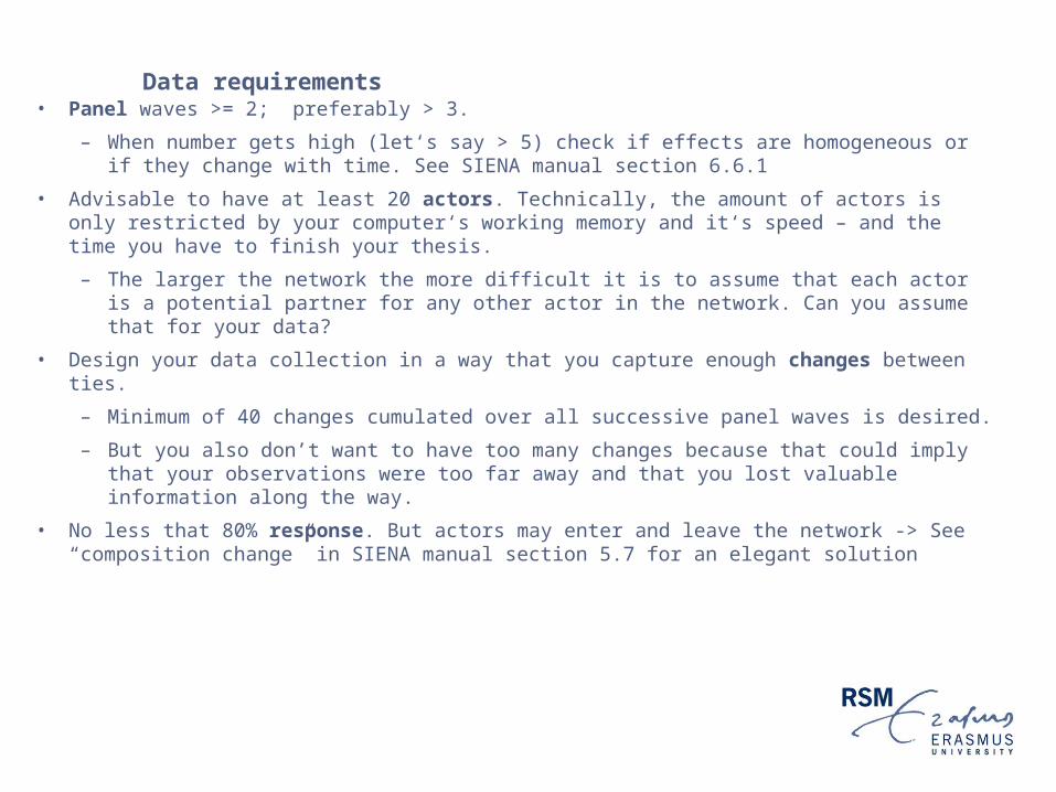
Data requirements• Panel waves >= 2; preferably > 3.
– When number gets high (let‘s say > 5) check if effects are homogeneous or if they change with time. See SIENA manual section 6.6.1
• Advisable to have at least 20 actors. Technically, the amount of actors is only restricted by your computer‘s working memory and it‘s speed – and the time you have to finish your thesis.
– The larger the network the more difficult it is to assume that each actor is a potential partner for any other actor in the network. Can you assume that for your data?
• Design your data collection in a way that you capture enough changes between ties.
– Minimum of 40 changes cumulated over all successive panel waves is desired.
– But you also don’t want to have too many changes because that could imply that your observations were too far away and that you lost valuable information along the way.
• No less that 80% response. But actors may enter and leave the network -> See “composition change” in SIENA manual section 5.7 for an elegant solution

Running SIENA
• This is done in 5 steps:
1. Data
2. Transformation
3. Selection
4. Model
5. Results
• Example here: van den Bunt friendship Data. Available at SIENA homepage

0. Getting started
•For starting a new project choose “Start with new project”
(who would have not guessed that?)

0. Getting started
When running SIENA for the first time you need to define directories where you store your file – after a first time installation StocNet might ask you to do this right away.

1. Data
• Network and covariate data have to be entered in .txt or .DAT files and have to be tab separated (consult SIENA manual section 5 for other options).
• There cannot be blanks
– Network files are adjacency matrices.
– Covariates are rows with as many rows as actors. Actors have the same order as in the network.
• Changing covariates: When number of observations is m then you need to include m-1 columns.
– Example: First column contains covariate at T1, which is then used to predict T2. Second column contains covariate at T2, which is used to predict T3, etc,….
• Constant covariate : File can contain multiple constant covariates (e.g., demographics of an actor). E.g, first column age; second column gender, etc.
– Dyadic variables: Enter in same format as network variables (adjacency matrix). Values between 0 – 255. Only integers.
• for changing dyadic variables you need m -1 variables.

1. Data
– Usually, you can copy/ paste from Ucinet/Excel into .txt files and it is automatically tab seperated.
– When using large data sets (several hundreds of actors) you might run into trouble when using Microsoft Notepad to manage .txt files. Use some other software (e.g., EditPad Lite ; its for free).

1. Data
1. Click “Add” to add network files in successive order
2. Choose the file (which you should already have stored in your dedicated network folder)
3. Click into the box to change the name of the network (e.g., 1, 2, 3 ,4 ,5, ..)
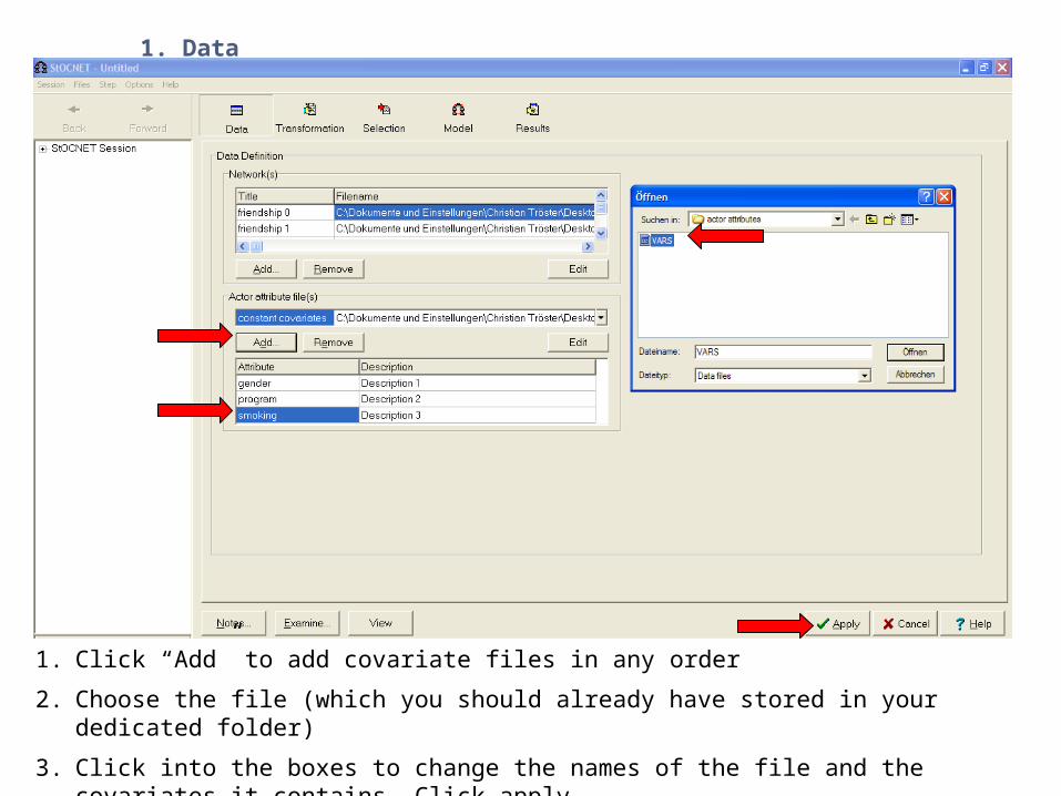
1. Data
1. Click “Add” to add covariate files in any order
2. Choose the file (which you should already have stored in your dedicated folder)
3. Click into the boxes to change the names of the file and the covariates it contains. Click apply

2. Transformation
• SIENA can only handle dichotomized networks (0 & 1)
– Work in progress: valued graphs might be possible in near future
• Indicate missing values
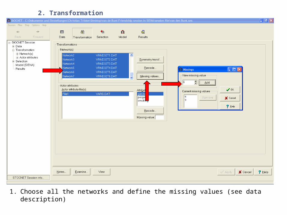
2. Transformation
1. Choose all the networks and define the missing values (see data description)

2. Transformation: Networks
1. Choose all the networks and click on “Recode”
2. Recode the network into 1 and 0 (see data description of example: 1 & 2 -> 1 & 3;4;5 -> 0)

2. Transformation: Attributes
1. Choose the covariate you want to recode and click on “Recode”
2. Recode the covariate into 1 and 0 (see data description: 1 & 2 -> 1 & 3;4;5 -> 0)

3. Selection
• Here you can remove actors from the analysis.
• Does not reflect social reality. Removing an actor in reality probably would affects whole network.
• If you want to test differences in effect for a range of actors use covariates (e.g. dummies)

4. Model: Data specification
• The networks
• Dyadic variables
• Constant covariates: E.g., gender
• Changing covariates:
– If endogenous then should be modeled as dependent variable (e.g., individuals’ performance)
– If exogenous then then treated as independent changing covariate
• Composition change. See manual section 5.7
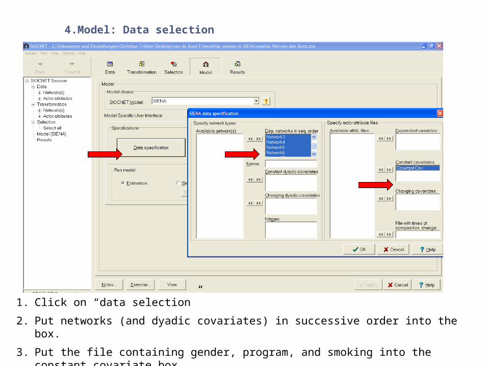
4.Model: Data selection
1. Click on “data selection”
2. Put networks (and dyadic covariates) in successive order into the box.
3. Put the file containing gender, program, and smoking into the constant covariate box

4.Model: Model specification
1. Click on “Model specification”
2. Choose the effects you want to test according to your theory. Check under “v”
3. Click “ok” and then “run” to start the estimation process
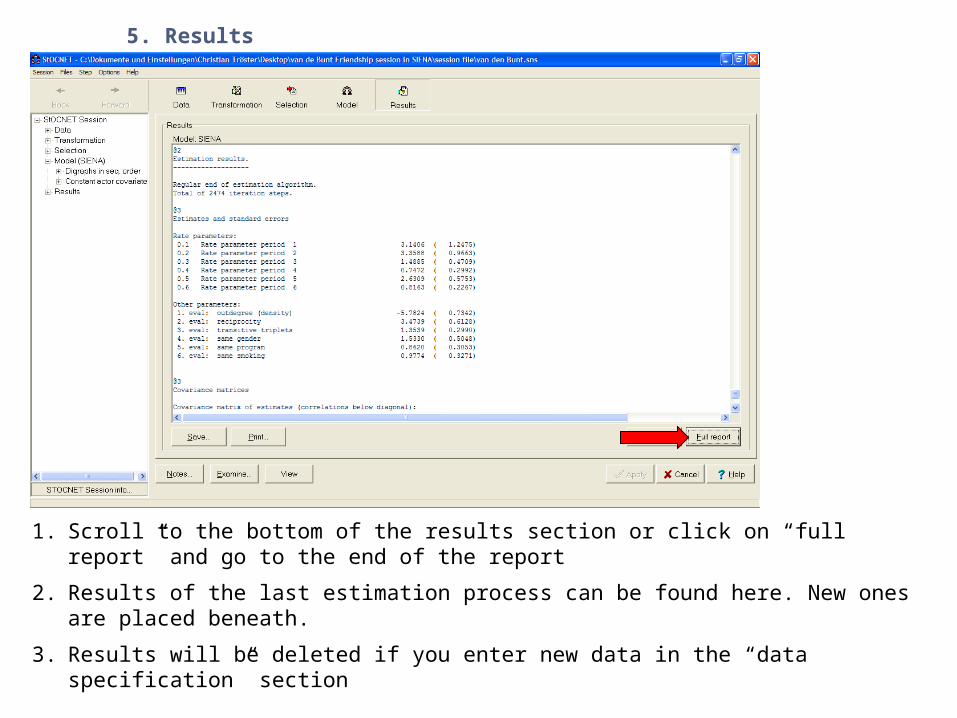
5. Results
1. Scroll to the bottom of the results section or click on “full report” and go to the end of the report
2. Results of the last estimation process can be found here. New ones are placed beneath.
3. Results will be deleted if you enter new data in the “data specification” section

5. Results
• Don’t jump to the parameter estimates first!
• First, check if convergence is good. That is, if your model describes your observed data well. If not, then you cannot trust the parameter estimates!
– Good convergence is indicated by t-rations close to zero
– t-rations below |0.1| indicate convergence.
• Check rate parameters: This are the unobserved changes an actor makes between two observations. You have to decide what is reasonable
– Remember: An actor can also decide to do nothing
• Significance of parameters / T-test: Divide the parameter by the standard error and look in a t-test table if the value is significant for an unlimited amount of degrees of freedom.
– Above 1.96 is significant for p < .05 two-tailed
• Parameters above 2 and certainly above 5 are doubtful.
• Check covariance/ correlation matrix.
– If you find high correlations they wont be problematic but might explain high standard errors in your parameters. In this case, you might exclude one of the two variables and re-run the estimation.

Improving your model:
• Bad convergence is probably due to a mis-specified model.
–You can add/remove effects. But again: This should be guided by theory.
–Increase the multiplication factor, e.g. to 10, then 15, then 20, etc.
–Decrease the initial value of gain parameter, e.g. to 0.01, then 0.001, etc.
–Increase the number of iterations (enough time to get a coffee…)
•Should be 2000 for results to be reported..
–One change at a time!
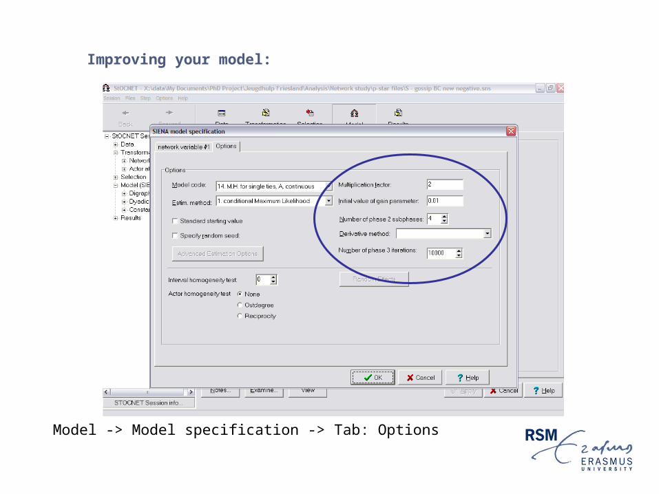
Improving your model:
Model -> Model specification -> Tab: Options

More advanced issues
• Evolution of covariates: Influence of ties or influence within networks
• Multilevel
• Endowment effects
• Interactions (between parameters, with time, rate parameter)
• Score type test -> SIENA manual section 9.1

Multilevel Analysis (SIENA manual section 14)
Meta Analysis Multi-Group Option Structural Zeros
Parameters are not constrained within Networks
Only rate parameters are not constrained within networks
All parameters are the same for all networks
Networks need to be of sufficient size
Networks are combined and, therefore, yield higher power
Networks are combined and, therefore, yield higher power
Can differ in number of observation moments
Can differ in number of observation moments
Need to have same amount of observation moments
* If one interacts sub-group dummies with rate parameters, same results as in multi-group option
Preferred method because makes less strict assumption
Preferred above “structural zero” approach with dummies because takes less time in SIENA
Least preferred

Useful information sources
• SIENA homepage http://stat.gamma.rug.nl/siena.html
• Yahoo StocNet user Group http://tech.groups.yahoo.com/group/stocnet/
Notes
• The literature on SIENA spends some effort in explaining relative effect size. However, in social sciences we are generally interested in the significance of an effect and not its relative effect size because adding or removing an effect would change the relative effect size….and how do we know we added all the effects that “truly” predict the network.


