Long-term trends in economicinequality: the case of the Florentine
state, c. 1300–1800†
By GUIDO ALFANI and FRANCESCO AMMANNATI∗
This article provides an overview of economic inequality, particularly of wealth, in theFlorentine state (Tuscany) from the early fourteenth to the late eighteenth century.Regional studies of this kind are rare, and this is only the second-ever attempt atcovering such a long period. Consistent with recent research conducted on otherEuropean areas, during the early modern period we find clear indications of a tendencyfor economic inequality to grow continually, a finding that for Tuscany cannot beexplained as the consequence of economic growth. Furthermore, the exceptionallyold sources we use allow us to demonstrate that a phase of declining inequality,lasting about one century, was triggered by the Black Death from 1348 to 1349. Thisfinding challenges earlier scholarship and significantly alters our understanding of theeconomic consequences of the Black Death.
I n recent years, research on economic inequality has seen significant change.First, in many countries the Great Recession that began in 2007 has altered the
perception of economic inequality—which has increasingly been seen as a problem,with a growing call for public action to moderate it. Second, the study of long-termdynamics has tended to become central to the analysis of current inequality levels.Although the most notable example of both trends is probably Piketty’s recentand controversial book,1 which calls for placing distribution back at the centreof economic analysis, it is only part of a more general process. If we focus onpost-2007 scholarship, regarding long-term dynamics it is interesting to note thatresearch covered not only the nineteenth and twentieth centuries—see in particularthe works co-authored by Piketty himself2 and Prados de la Escosura’s studies ofSpain and Latin America3—but also, and with maybe even greater frequency, thepre-industrial period. Areas covered by recent studies include the Sabaudian state
* Authors’ Affiliations: Guido Alfani, PAM—Bocconi University, Dondena Centre, and IGIER; FrancescoAmmannati Bocconi University, Dondena Centre.† We thank Conchita D’Ambrosio, Richard Goldthwaite, Paolo Malanima, Branko Milanovic, Tommy Murphy,John Padgett, Marco Percoco, Giuliano Pinto, Jaime Reis, Wouter Ryckbosch, Francesco Scalone, FedericoTadei, participants at the conference session ‘Economic inequality and population dynamics’ (European SocialScience History Conference, Vienna, Austria, April 2014) and seminar participants at Bocconi University, at theUniversity of Pisa, and at Utrecht University for their many helpful comments. Sections I to III were mostly writtenby Francesco Ammannati, and IV to VI by Guido Alfani, while the introduction and section VII were writtentogether. The research leading to these results has received funding from the European Research Council underthe European Union’s Seventh Framework Programme (FP7/2007–2013)/ERC grant agreement no. 283802,EINITE–Economic Inequality across Italy and Europe, 1300–1800.
1 Piketty, Capital.2 Atkinson, Picketty, and Saez, ‘Top incomes’; Alvaredo, Atkinson, Picketty, and Saez, ‘Top 1 percent’.3 Prados de la Escosura, ‘Inequality and poverty’; idem, ‘Kuznets curve’.
in north-western Italy,4 the Low Countries,5 Spain,6 Portugal,7 and Turkey.8 Allthis research is characterized by the use of new databases built from fresh archivalresearch. To these, the paper by Milanovic et al.9 which introduced the notion ofthe ‘inequality possibility frontier’ should be added, as well as Hoffman et al.’sstudy of ‘real’ inequality in Europe (a concept also applied by Hanus to his recentstudy of ’s-Hertogenbosch in the Low Countries).10
The change in focus towards the preindustrial period is an interestingdevelopment, considering that before 2007 the only study of long-term trendsin pre-industrial economic inequality based on quantitative data was van Zanden’sanalysis of the Dutch Republic.11 This work made reference to Kuznets’s originalhypothesis, according to which income inequality would follow an inverted-Upath through the industrialization process (the so-called ‘Kuznets curve’), witha rising phase at the beginning of industrialization.12 Van Zanden suggested thata ‘super-Kuznets curve’ could be described for the Dutch Republic, connectingpre-industrial and industrial economic growth. His study was an exception, in afield in which most research generated by Kuznets’s seminal paper focused onthe industrialization period.13 However, Kuznets’s ideas are currently the objectof deep criticism, especially regarding his ‘promise’ of declining inequality whichseems not to have been fulfilled by actual historical developments.14 The notionof a super-Kuznets curve has been criticized, too, in at least two respects: first,as was originally hypothesized by Alfani in his study of the Sabaudian state, inthe long run substantial inequality growth (especially of wealth) can also be foundin stagnating or declining areas of Europe (requiring us to individuate drivers ofinequality growth different from economic growth);15 and second, as argued byReis, the paradigm of the super-Kuznets curve does not apply to the whole ofEurope. Particularly in Portugal, income inequality declined during most of theearly modern period.16
All recent revisionist work has called for more empirical research, as the amountof information we have about long-term inequality trends is still fairly limited.Our article contributes to this general debate by developing the case study of theFlorentine state which covered most of Tuscany and was not only one of the mainpre-Unification Italian states, but also one that occupied a truly central positionin the medieval European economy. The methods we use are meant to make our
5 Ryckbosch, ‘Consumer revolution’; idem, ‘Economic inequality’; Hanus, ‘Real inequality’.6 Nicolini and Ramos Palencia, ‘Comparing income and wealth inequality’; Santiago-Caballero, ‘Income’;
Santiago-Caballero and Fernandez, ‘Income inequality in Madrid’; Garcia Montero, ‘Long-term trends’.7 Reis, ‘Deviant behaviour?’.8 Canbakal, Wealth.9 Milanovic, Lindert, and Williamson, ‘Pre-industrial inequality’.
10 Hoffman, Jacks, Levin, and Lindert, ‘Real inequality’; Hanus, ‘Real inequality’.11 van Zanden, ‘Tracing’; Soltow and van Zanden, Income.12 Kuznets, ‘Economic growth’.13 For example, Williamson, British capitalism, for Britain; Picketty, Postel-Vinay, and Rosenthal, ‘Wealth’, for
France; Rossi, Toniolo, and Vecchi, ‘Kuznets curve’, for Italy; Lindert and Williamson, American inequality, forthe US.
case study as comparable as possible to Alfani’s work on Piedmont/the Sabaudianstate, as well as to other research currently underway for other regions of Italy andEurope. The exceptional sources available for the Tuscan area allow us to cover aparticularly long period, from the early fourteenth to the late eighteenth century.We contribute to the current critical debate on the super-Kuznets curve, as in thecase of Tuscany, too, substantial inequality growth was found both in periods ofeconomic growth and stagnation.
I
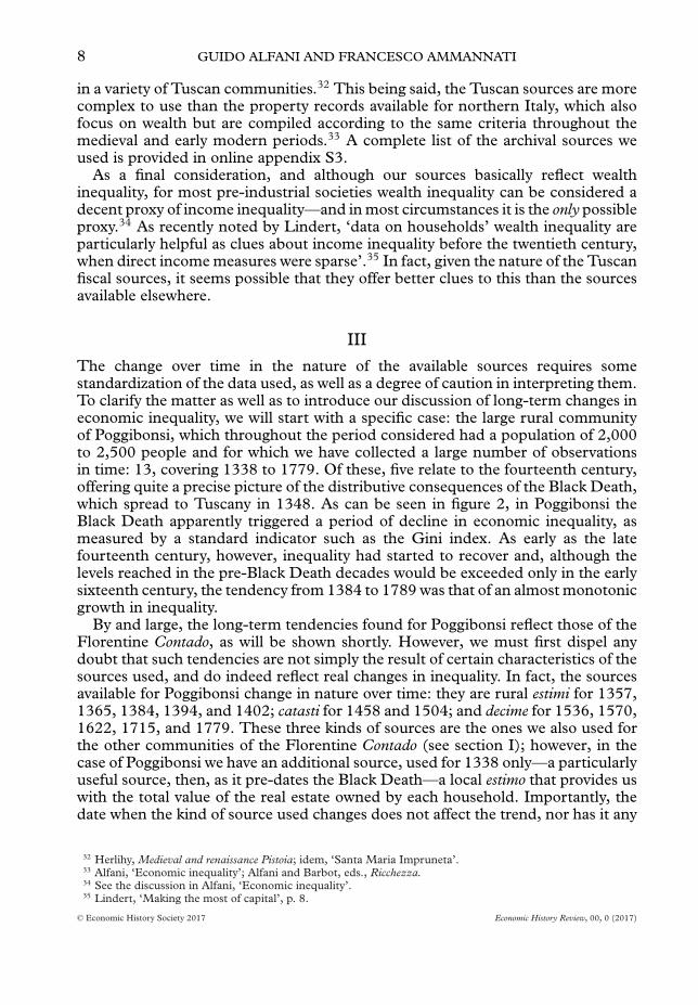
The ‘Tuscany’ considered in this work does not coincide exactly with the presentadministrative region, as we do not cover the Republic of Lucca, and a series ofterritories that were annexed during the eighteenth century.17 The area we studycorresponds to the territory of the Republic of Florence with its developmentinto the Duchy (from 1532) and subsequently the Grand Duchy (from 1569) ofTuscany. This large area was split into two parts administratively, differing both forthe intensity of the political control exerted by the capital city of Florence and forthe system of taxation. The Contado was the surrounding hinterland that originallyembraced the dioceses of Florence and Fiesole and then expanded as Florencebrought more territory under its control. Later, when larger cities like Arezzo andPisa came under Florentine rule together with their rural territories (in 1384 and1406 respectively), they were referred to as the Distretto.
From the fiscal standpoint, the distinction between Contado and Distretto wasmaintained until the eighteenth century, not only because of the existence of aseries of gabelle (‘duties’), but primarily for the different systems of direct taxationin force over the two areas. The Contado consisted of more than 1,100 mediumand small communities all under a single fiscal system set up by Florence which,however, suffered some major changes during the period considered. From 1315Florentine citizens were spared direct taxation based on the estimo, and it was keptonly for the communities of the Contado. The capital was subject to indirect taxationand forced loans.18 Athough evidence exists of estimi for the Contado dating backto 1259,19 the first surviving ones are those of 1350. From 1350 to 1415 therewere eight revisions of the estimo of the Florentine Contado: 1350, 1357, 1364–5, 1372–3, 1384, 1394, 1401–2, and 1412–15. The determination of the quotad’estimo—that is, the amount due from each taxpayer—took place in two stages:once the overall amount to be imposed on the whole Contado was established,by law ‘Officers of the estimo’ were given the mandate to distribute it among thevarious communities. The quota was then split between the households of eachsingle community on the basis of an evaluation of the household’s approximatedability to pay. Such evaluation was mostly based on the real estate (lands andbuildings) owned by each household.
The estimo represented a significant technical advance compared to the previousforms of taxation based on the feudal focatico at a fixed value. However, in 1427Florence introduced its famous catasto, a complex and very innovative attempt to
17 Fasano Guarini, Lo stato.18 Barbadoro, Le finanze.19 Conti, I catasti.
change the state’s fiscal policy in favour of a better and more efficient distributionof taxation.20 In May 1428 the law was extended to the Contado: here the catastowas renewed in 1435–7, 1451–5, 1458–60, 1469–71, 1487–90 and 1504–5 and itwas prepared in accordance with the same criteria as used for the city, representinga clear improvement over the estimi, which had become increasingly complex tomanage. The sum expressed in the catasto was the capital value: the propertywas valued by capitalizing the income declared (in kind for land, in cash forrents of urban properties) at the rate of 7 per cent, and the house of residencewas excluded. Household goods, commodities, credits, and debts also had to bereported. The difference between assets and liabilities formed the ‘sustanze’ or‘valsente’ (‘patrimony’ or ‘capital’) that was taxed. Although in theory the catastoinvolved a very wide and varied tax base, in practice after 1427 the system becamemuch simpler. In all subsequent catasti, almost always only real estate was recorded,and this is definitely the case for all the archival sources we consulted. Accordingto Conti, ‘in the registers of the countryside it is possible to see, after 1427, agradual deterioration of the assessments . . . Livestock, credits, traffici, and anyother easily concealable property rarefy or disappear entirely in the new surveys’.21
The reason for this development is presumably that ‘no financial administrationwould have been able, given the technical means of the time, to exert a trulyeffective control over the multifaceted rural world. What could be improved werethe records of landed property’.22 This problem was not limited to the country. Itwas also encountered in the city, and in fact, from the 1440s urban assessments, itceased to show movable goods and components of wealth other than real estate.23
As a matter of fact, these developments prepared the introduction, in 1495, of anew, simpler system of taxation that was based on the decima, an annual tax of 10per cent (hence the name) to be applied to the income from immovable propertyowned by citizens and peasants. The house of residence was exempted. In thecountryside the decima was introduced only from 1507–8, while in 1516 Pope LeoX granted the extension of taxation to ecclesiastical property, albeit restricted tothe assets purchased after that date.24 The introduction of the decima system ledto a complete replacement, in both the city and the countryside, of the previousregisters by a direct survey of all real estate. The decima was abolished in 1776.Contextually, however, each community was ordered to survey the assets situated intheir territory and to collect the decima one last time (in 1779). As a final commenton these sources, it should be noted that as the post-1427 catasti and the decimado not include financial assets, which tended to be more unevenly distributedthan real estate, inequality measures calculated from them have to be considered alower-bound estimate of overall wealth inequality. As financial assets tended to beconcentrated in the hands of city dwellers, this is mostly a problem when estimatingurban inequality. However, this also means that after 1427 there will be a systematicunderestimation of urban–rural differentials in inequality levels.25
20 Herlihy and Klapisch-Zuber, Tuscans.21 Conti, I catasti, p. 114, our translation.22 Ibid., p. 117, our translation.23 Procacci, Studio, pp. 62–6.24 Conti, I catasti, p. 132; Procacci, Studio, pp. 75–9.25 Regarding the distribution of financial assets in 1427 Tuscany, see Herlihy, ‘Family’.
Regarding the Distretto, each main centre had its own tax system that levied taxboth within the city walls and in the countryside. The Florentine fiscal policy aimedto leave each main centre some freedom in the choice of the tax system, merelyrequiring periodic global contributions. A fiscal study of the cities belonging to theDistretto therefore requires analytical work on a case-by-case basis. This is presentedin online appendix S1.26
II
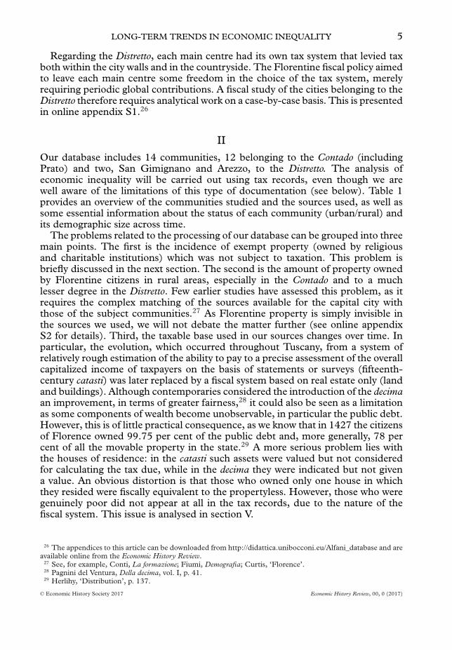
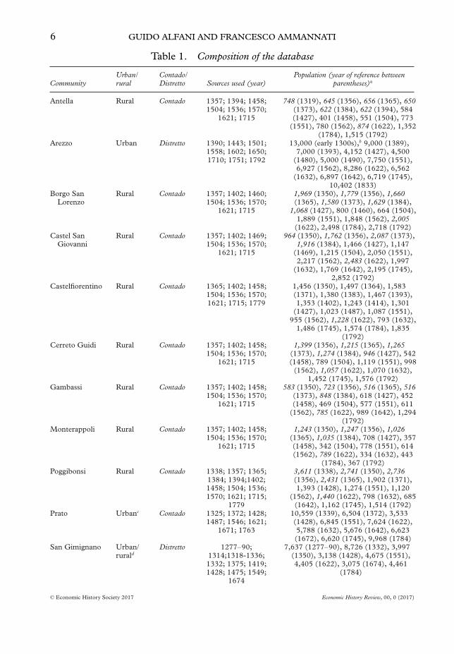
Our database includes 14 communities, 12 belonging to the Contado (includingPrato) and two, San Gimignano and Arezzo, to the Distretto. The analysis ofeconomic inequality will be carried out using tax records, even though we arewell aware of the limitations of this type of documentation (see below). Table 1provides an overview of the communities studied and the sources used, as well assome essential information about the status of each community (urban/rural) andits demographic size across time.
The problems related to the processing of our database can be grouped into threemain points. The first is the incidence of exempt property (owned by religiousand charitable institutions) which was not subject to taxation. This problem isbriefly discussed in the next section. The second is the amount of property ownedby Florentine citizens in rural areas, especially in the Contado and to a muchlesser degree in the Distretto. Few earlier studies have assessed this problem, as itrequires the complex matching of the sources available for the capital city withthose of the subject communities.27 As Florentine property is simply invisible inthe sources we used, we will not debate the matter further (see online appendixS2 for details). Third, the taxable base used in our sources changes over time. Inparticular, the evolution, which occurred throughout Tuscany, from a system ofrelatively rough estimation of the ability to pay to a precise assessment of the overallcapitalized income of taxpayers on the basis of statements or surveys (fifteenth-century catasti) was later replaced by a fiscal system based on real estate only (landand buildings). Although contemporaries considered the introduction of the decimaan improvement, in terms of greater fairness,28 it could also be seen as a limitationas some components of wealth become unobservable, in particular the public debt.However, this is of little practical consequence, as we know that in 1427 the citizensof Florence owned 99.75 per cent of the public debt and, more generally, 78 percent of all the movable property in the state.29 A more serious problem lies withthe houses of residence: in the catasti such assets were valued but not consideredfor calculating the tax due, while in the decima they were indicated but not givena value. An obvious distortion is that those who owned only one house in whichthey resided were fiscally equivalent to the propertyless. However, those who weregenuinely poor did not appear at all in the tax records, due to the nature of thefiscal system. This issue is analysed in section V.
26 The appendices to this article can be downloaded from http://didattica.unibocconi.eu/Alfani_database and areavailable online from the Economic History Review.
27 See, for example, Conti, La formazione; Fiumi, Demografia; Curtis, ‘Florence’.28 Pagnini del Ventura, Della decima, vol. I, p. 41.29 Herlihy, ‘Distribution’, p. 137.
Notes and sources:a Our own estimates from archival documentation, integrated with figures published by Dini, Arezzo, and del Panta, Una traccia,for Arezzo and Prato; Fiumi, Storia economica, and idem, Demografia, for San Gimignano and Prato; Fiumi, ‘La demografia’, andConti, La formazione, for the Contado of Florence. In italics: (a) our estimates obtained by multiplying the number of hearths bythe average size of a hearth according to the fiscal data of each community of the Contado for the breakpoint years 1450 and 1500(and, when available, for 1427), or (b) only for 1622, our estimates obtained by multiplying the population in 1562 (in 1551 forSanta Maria Impruneta and San Godenzo) by the average growth rate of the relevant vicariato (each vicariato included a group ofrural communities).b Uncertain estimate.c An important centre of the valley of the Bisenzio, Prato and the rural areas under its jurisdiction became part of the Contadoof Florence after it was annexed in 1351. In the earlier periods, Prato was not formally a ‘city’ as its territory fell under thejurisdiction of the Diocese of Pistoia. Only in 1653 did Prato become an episcopal see.d City + countryside. Data from Fiumi, Storia economica, p. 174.
Before proceeding, the nature of the information we used to measure inequalityneeds further clarification. All of our sources (estimi, catasti, and decime) record thefiscal capacity of the taxpayers—that is, they tend to reflect their actual ability to paytax. From this point of view, there is consistency over time in the kind of informationthey provide, a conclusion further strengthened by the fact that changes in thesources used do not mark structural breaks in our series of inequality measures(see the next section). However, one might wonder whether our sources provideinformation about ‘wealth’ or ‘income’. A consolidated historiographic traditionhas assimilated the ‘capitalized income’ recorded by the catasti to wealth,30 withgood reasons: as shown by Lindert, although it is possible to use the catasto (atleast the first and most detailed one, in 1427) to estimate income inequality, anumber of hypotheses and related transformations have to be made.31 It is alsoclear that the decime record wealth (or more precisely, its main component: realestate), and as a matter of fact, the tax base of the catasti following the 1427 onewas very similar to that of the decime, especially in rural communities. Regardingthe estimi, earlier literature considered them directly comparable to the catasti, asthe evaluations they reported were based mostly on the real estate owned by eachhousehold. Herlihy in particular used them explicitly to study wealth distribution
30 Ibid.; Herlihy and Klapisch-Zuber, Tuscans.31 Milanovic et al., ‘Pre-industrial inequality’, p. 269.
in a variety of Tuscan communities.32 This being said, the Tuscan sources are morecomplex to use than the property records available for northern Italy, which alsofocus on wealth but are compiled according to the same criteria throughout themedieval and early modern periods.33 A complete list of the archival sources weused is provided in online appendix S3.
As a final consideration, and although our sources basically reflect wealthinequality, for most pre-industrial societies wealth inequality can be considered adecent proxy of income inequality—and in most circumstances it is the only possibleproxy.34 As recently noted by Lindert, ‘data on households’ wealth inequality areparticularly helpful as clues about income inequality before the twentieth century,when direct income measures were sparse’.35 In fact, given the nature of the Tuscanfiscal sources, it seems possible that they offer better clues to this than the sourcesavailable elsewhere.
III
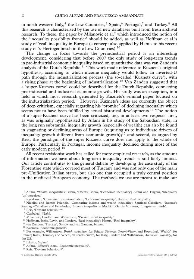
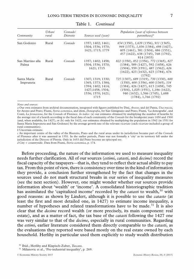
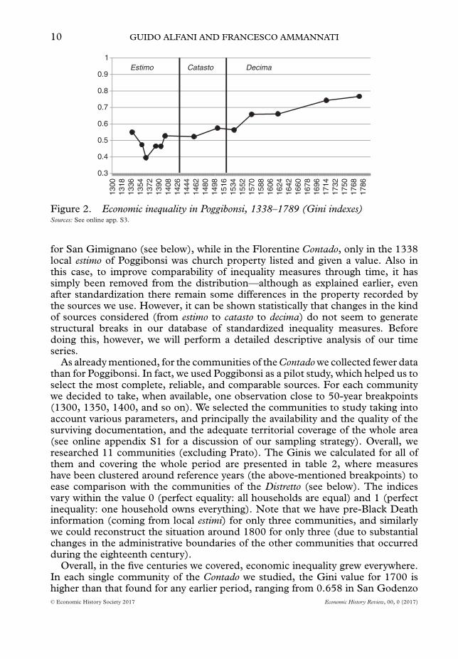
The change over time in the nature of the available sources requires somestandardization of the data used, as well as a degree of caution in interpreting them.To clarify the matter as well as to introduce our discussion of long-term changes ineconomic inequality, we will start with a specific case: the large rural communityof Poggibonsi, which throughout the period considered had a population of 2,000to 2,500 people and for which we have collected a large number of observationsin time: 13, covering 1338 to 1779. Of these, five relate to the fourteenth century,offering quite a precise picture of the distributive consequences of the Black Death,which spread to Tuscany in 1348. As can be seen in figure 2, in Poggibonsi theBlack Death apparently triggered a period of decline in economic inequality, asmeasured by a standard indicator such as the Gini index. As early as the latefourteenth century, however, inequality had started to recover and, although thelevels reached in the pre-Black Death decades would be exceeded only in the earlysixteenth century, the tendency from 1384 to 1789 was that of an almost monotonicgrowth in inequality.
By and large, the long-term tendencies found for Poggibonsi reflect those of theFlorentine Contado, as will be shown shortly. However, we must first dispel anydoubt that such tendencies are not simply the result of certain characteristics of thesources used, and do indeed reflect real changes in inequality. In fact, the sourcesavailable for Poggibonsi change in nature over time: they are rural estimi for 1357,1365, 1384, 1394, and 1402; catasti for 1458 and 1504; and decime for 1536, 1570,1622, 1715, and 1779. These three kinds of sources are the ones we also used forthe other communities of the Florentine Contado (see section I); however, in thecase of Poggibonsi we have an additional source, used for 1338 only—a particularlyuseful source, then, as it pre-dates the Black Death—a local estimo that provides uswith the total value of the real estate owned by each household. Importantly, thedate when the kind of source used changes does not affect the trend, nor has it any
32 Herlihy, Medieval and renaissance Pistoia; idem, ‘Santa Maria Impruneta’.33 Alfani, ‘Economic inequality’; Alfani and Barbot, eds., Ricchezza.34 See the discussion in Alfani, ‘Economic inequality’.35 Lindert, ‘Making the most of capital’, p. 8.
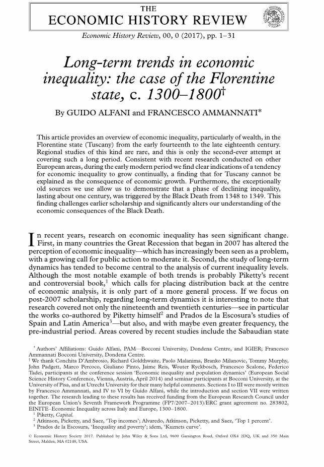
Figure 1. The Florentine state: Contado and Distretto (c. 1406)Note: Only the communities included in our analysis, plus the capital city of Florence, are indicated on the map.
significant impact on the level of the Gini index. It is true that a minimal declinein the Gini level is found between 1402 and 1458 and between 1504 and 1536,but this does not change the overall long-term tendency of inequality to grow. Theless homogeneous source is probably the 1338 local estimo but in this case too, thetendency from 1338 to 1357 seems to continue from 1357 to 1365, so we have noreason to suspect that it is not genuine.
Figure 2. Economic inequality in Poggibonsi, 1338–1789 (Gini indexes)Sources: See online app. S3.
for San Gimignano (see below), while in the Florentine Contado, only in the 1338local estimo of Poggibonsi was church property listed and given a value. Also inthis case, to improve comparability of inequality measures through time, it hassimply been removed from the distribution—although as explained earlier, evenafter standardization there remain some differences in the property recorded bythe sources we use. However, it can be shown statistically that changes in the kindof sources considered (from estimo to catasto to decima) do not seem to generatestructural breaks in our database of standardized inequality measures. Beforedoing this, however, we will perform a detailed descriptive analysis of our timeseries.
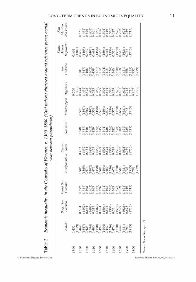
As already mentioned, for the communities of the Contado we collected fewer datathan for Poggibonsi. In fact, we used Poggibonsi as a pilot study, which helped us toselect the most complete, reliable, and comparable sources. For each communitywe decided to take, when available, one observation close to 50-year breakpoints(1300, 1350, 1400, and so on). We selected the communities to study taking intoaccount various parameters, and principally the availability and the quality of thesurviving documentation, and the adequate territorial coverage of the whole area(see online appendix S1 for a discussion of our sampling strategy). Overall, weresearched 11 communities (excluding Prato). The Ginis we calculated for all ofthem and covering the whole period are presented in table 2, where measureshave been clustered around reference years (the above-mentioned breakpoints) toease comparison with the communities of the Distretto (see below). The indicesvary within the value 0 (perfect equality: all households are equal) and 1 (perfectinequality: one household owns everything). Note that we have pre-Black Deathinformation (coming from local estimi) for only three communities, and similarlywe could reconstruct the situation around 1800 for only three (due to substantialchanges in the administrative boundaries of the other communities that occurredduring the eighteenth century).
to 0.939 in San Martino alla Palma. On the whole, these values are similar to theGinis measured for rural areas in other parts of Italy. For example, in Piedmontaround the same date, the Gini was 0.579 in Cumiana and 0.733 in Vigone.36 Inthese communities, like in San Godenzo, Poggibonsi, and Castelfiorentino wherethe Gini rose respectively to 0.752, 0.767, and 0.788 by 1779, inequality continuedto grow during the eighteenth century, to 0.675 in Cumiana by 1749 and to 0.809in Vigone by 1764. In another part of Italy, Romagna, in 1783 rural Ginis were inthe range 0.76–0.82 in the territory of Brisighella and 0.67–0.75 in that of Russi.37
Both for Piedmont and Romagna, the measures refer to inequality in ownership ofreal estate (excluding the propertyless), and can be cautiously compared with thosewe provide based on the decima. Consequently, our communities do not seem tobe exceptional from the point of view of inequality levels, save for San Martinoalla Palma, where the Gini for 1700 equals 0.939 (in fact, from around 1550 SanMartino is invariably the most unequal community). This very high level—thehighest found to date in any Italian rural community at any time—could be due tospecific dynamics affecting this community, particularly its apparent de-populationover time (as reflected in the steady decline in the number of recorded taxpayers:from more than 100 until the early sixteenth century, to a few scores in the finaldates) with consequent extreme concentration of local real estate in few ‘surviving’hands. It should also be noted that such a high level of rural inequality is notaltogether unrealistic, as similar levels are attested to in other areas of Europe (forexample, the real estate Gini was 0.92 in the French village of Saint-Etienne-de-Bailleul in 1826).38
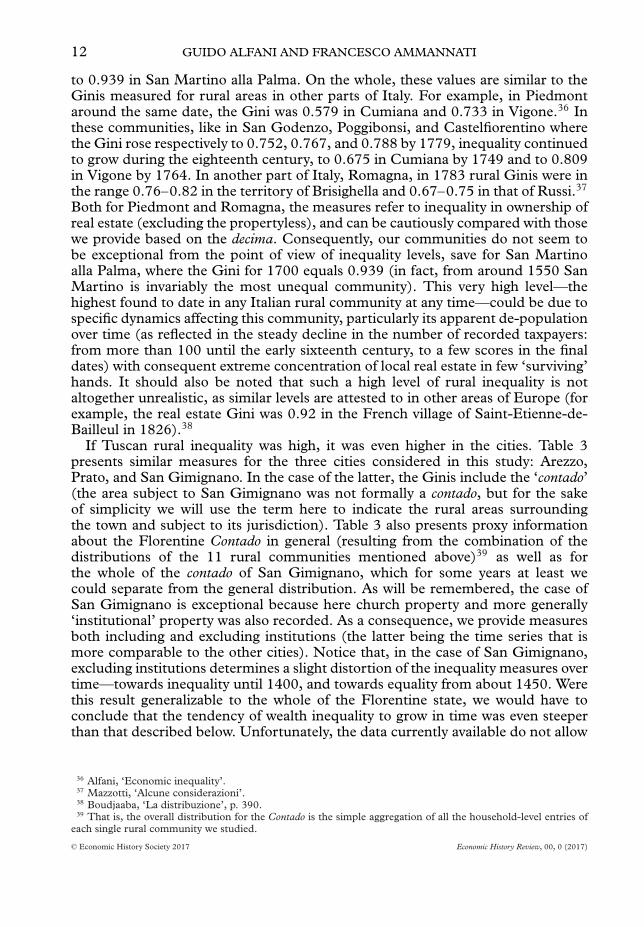
If Tuscan rural inequality was high, it was even higher in the cities. Table 3presents similar measures for the three cities considered in this study: Arezzo,Prato, and San Gimignano. In the case of the latter, the Ginis include the ‘contado’(the area subject to San Gimignano was not formally a contado, but for the sakeof simplicity we will use the term here to indicate the rural areas surroundingthe town and subject to its jurisdiction). Table 3 also presents proxy informationabout the Florentine Contado in general (resulting from the combination of thedistributions of the 11 rural communities mentioned above)39 as well as forthe whole of the contado of San Gimignano, which for some years at least wecould separate from the general distribution. As will be remembered, the case ofSan Gimignano is exceptional because here church property and more generally‘institutional’ property was also recorded. As a consequence, we provide measuresboth including and excluding institutions (the latter being the time series that ismore comparable to the other cities). Notice that, in the case of San Gimignano,excluding institutions determines a slight distortion of the inequality measures overtime—towards inequality until 1400, and towards equality from about 1450. Werethis result generalizable to the whole of the Florentine state, we would have toconclude that the tendency of wealth inequality to grow in time was even steeperthan that described below. Unfortunately, the data currently available do not allow
36 Alfani, ‘Economic inequality’.37 Mazzotti, ‘Alcune considerazioni’.38 Boudjaaba, ‘La distribuzione’, p. 390.39 That is, the overall distribution for the Contado is the simple aggregation of all the household-level entries of
Table 3. Economic inequality in selected areas of Tuscany, c. 1300–1800 (Giniindices clustered around reference years; actual year between parentheses)
Arezzo Prato
San Gimignano(including the
contado)
San Gimignano(including the contado,excluding institutions)
Contado of SanGimignano
Contado ofFlorence
1300 0.703(1325)
0.712 (1277–90) 0.674 (1290)
1350 0.591(1372)
0.657 (1375) 0.658 (1375) 0.585 (1375) 0.53
1400 0.481(1390)
0.634 (1419) 0.639 (1419) 0.499 (1419) 0.57
1450 0.600(1443)
0.683(1428)
0.674 (1428) 0.671 (1428) 0.504
1500 0.627(1501)
0.624(1487)
0.648 (1475) 0.631 (1475) 0.582 (1475) 0.546
1550 0.651(1558)
0.575(1546)
0.627 (1549) 0.592 (1549) 0.630 (1549) 0.540
1600 0.722(1602)
0.737(1621)
0.613
1650 0.725(1650)
0.807(1671)
0.682 (1674) 0.641 (1674) 0.645
1700 0.810(1710)
0.737
1750 0.846(1751)
0.831(1763)
1800 0.832(1792)
0.855a
(1779)
Note: a Measure calculated from three communities out of 11.Sources: See online app. S3.
us to test such a hypothesis—consequently, also for reasons of synthesis, we willnot discuss the issue of church property further.
The data presented in tables 2 and 3 allow for some general considerationsabout the relative inequality levels in different Tuscan environments. There was,in fact, an earlier attempt to do this: Herlihy’s rightly famous study of economicinequality in the Florentine state.40 This study was based on a single source,the catasto of 1427. Herlihy reached a number of relevant conclusions. First,for cities, there exists a positive correlation between population size, averageper capita wealth, and concentration of property. In fact, in the smaller citiesunder Florentine rule (Cortona, Volterra, Prato) average per capita wealth wasabout 45 fiorini versus the 70–85 of medium-sized cities like Arezzo, Pistoia,and Pisa and the 273 of the capital city, Florence, where the richest familiesresided. Moreover, the Gini was higher in the capital (0.788) than in all othercities (0.747 in the aforementioned six cities taken together—unfortunately city-per-city measures are not provided),41 declining, as a tendency, with population.Second, when comparing inequality in cities and in rural communities, the firstwere almost invariably wealthier (in per capita terms) and more unequal. Accordingto Herlihy, average rural wealth equalled 32 fiorini per capita in the villages,
40 Herlihy, ‘Distribution’.41 Ibid., pp. 136–9; Herlihy and Klapisch-Zuber, Tuscans, p. 341.
and just 14 in sparsely populated areas.42 Although Herlihy did not calculateconcentration indexes for rural communities in the Contado of Florence, in hisstudy of the village of Santa Maria Impruneta he underlined the fact that theshare of wealth owned by the poorest 50 per cent of the population was aboutdouble in the country compared to Florence (6 per cent versus 2.68 per cent).43
We can add considerably to this comparison, as our database suggests that around1450 the Ginis for rural communities ranged from 0.429 (Gambassi) to 0.523(Poggibonsi)—considerably lower than the 0.600 found for Arezzo, 0.683 for Prato,and 0.671 for San Gimignano. A similar urban–rural differential is to be found inthe territory of Pistoia in the Florentine Distretto. Here, in 1427 the city had aGini of 0.713, while rural inequality varied between 0.634 for the villages on theplain taken together and 0.515 for those in the mountains.44 Finally, in Livorno,which at the time was still a small town with less than 7 per cent of the householdsof Pisa and about 1 per cent of those in Florence, a study reported a Gini of0.520.45
Herlihy’s pioneering intuitions were fundamentally right, but his analysis lackedlong-term perspective. This not only prevented him from noticing other interestingand important phenomena but also (and surely, independently from Herlihy’sintentions) it helped to spread the idea among international scholars that the 1427catasto was an exceptional source, the like of which was not to be found in anyother place, or at any other time. However, although it is true that the 1427 catastois particularly informative about many components of wealth, not-too-differentsources also exist for other parts of Italy and Europe that allow for a systematicstudy of economic inequality and wealth or income distribution, as demonstratedby the recent case study of Piedmont46 as well as research on various Italiancommunities.47 Moreover, exceptional sources providing information as rich asthe catasto exist elsewhere, such as the 1613 Sabaudian ‘census’.48 Regarding theavailability of sources across time, Tuscan records redacted with criteria similarto the 1427 catasto cover a much longer period of about one century (the lastwe used for the Contado dates from 1504) and, as the data presented here show,other sources can be used in addition to produce information comparable in manyregards to that provided by the catasto, covering many centuries.
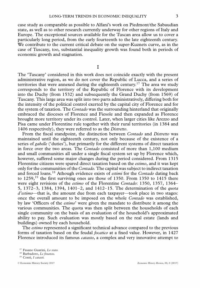
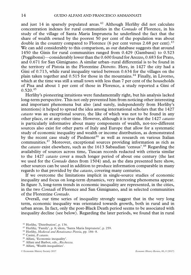
If we overcome the limitations implicit in single-source studies of economicinequality and focus on long-term dynamics, very interesting phenomena appear.In figure 3, long-term trends in economic inequality are represented, in the cities,in the two Contadi of Florence and San Gimignano, and in selected communitiesof the Florentine Contado.
Overall, our time series of inequality strongly suggest that in the very longterm, economic inequality was orientated towards growth, both in rural and inurban areas. In fact, only the post-Black Death period seems to be associated withinequality decline (see below). Regarding the later periods, we found that in rural
42 Herlihy, ‘Distribution’, p. 136.43 Herlihy, ‘Family’, p. 8; idem, ‘Santa Maria Impruneta’, p. 259.44 Herlihy, Medieval and Renaissance Pistoia, pp. 186–8.45 Casini, Il catasto.46 Alfani, ‘Economic inequality’.47 Alfani and Barbot, eds., Ricchezza.48 Alfani, ‘Wealth inequalities’.
Arezzo Prato San Gimignano (with contado, without institutions)
0.3
0.4
0.5
0.6
0.7
0.8
0.9
1
18001750170016501600155015001450140013501300
Castelfiorentino Poggibonsi
San Godenzo Santa Maria Impruneta
Contado of Florence Contado of St. Gimignano
Figure 3. Long-term trends in economic inequality (Gini indexes)[Colour figure can be viewed at wileyonlinelibrary.com]Sources: See online app. S3.
communities, from about 1450 inequality tended to grow almost monotonically.In the overall Florentine Contado, inequality stagnated or slightly declined onlyfrom 1500 to 1550, while continuing to rise in the contado of San Gimignano. Inthe cities the situation is more complex. In fact, although from about 1400 theoverall tendency is towards an increase in inequality, the process is much morelinear in Arezzo than in Prato or San Gimignano. While for San Gimignano theabsence of information after 1650 complicates the interpretation of the data, forPrato the impression is that the century from 1450 to 1550 marks the temporaryinterruption of an overarching process of increasing inequality spanning a muchlonger period. This could be partly the consequence of the terrible sack sufferedby the city in 1512, which cost the lives of many citizens and peasants49 and, as the
rich were usually targeted in such instances as the better able to provide bountyand ransoms,50 could have caused a downward levelling of the wealth distribution.Inequality decline, however, was already underway before the sack (the Gini indexdiminished from 0.683 in 1428 to 0.624 in 1487, before reaching a floor of 0.575in 1546).
Our urban time series also allow us to explore in some detail the relationshipbetween population growth and inequality growth. On the one hand our data largelyconfirm Herlihy’s intuition that smaller centres were less unequal than the largerones. Around 1427 (the date to which Herlihy referred), all our communities wereless unequal than the capital, Florence, and all cities were more unequal than thevillages of the Florentine Contado. Importantly, the second finding also remains trueat other points in time, as for 1407 we could calculate the Gini for a larger city, Pisa,whose value of 0.640 is higher than that which we found at similar dates in all othercases we studied. However, within the group of cities we studied, the hierarchy ofinequality levels does not match univocally that of population size (Arezzo, whichin the first half of the fifteenth century was the largest city in our database, is theleast unequal), a fact that could reflect differences both in local socio-economicstructures and the sources used. On the other hand, considering the developmentof each specific city or rural community, we find that the correlation betweenpopulation growth and inequality growth seems weaker than reported by studiesinvolving other areas, from Piedmont to Veneto,51 and as also confirmed by ourregression analysis (section VI).
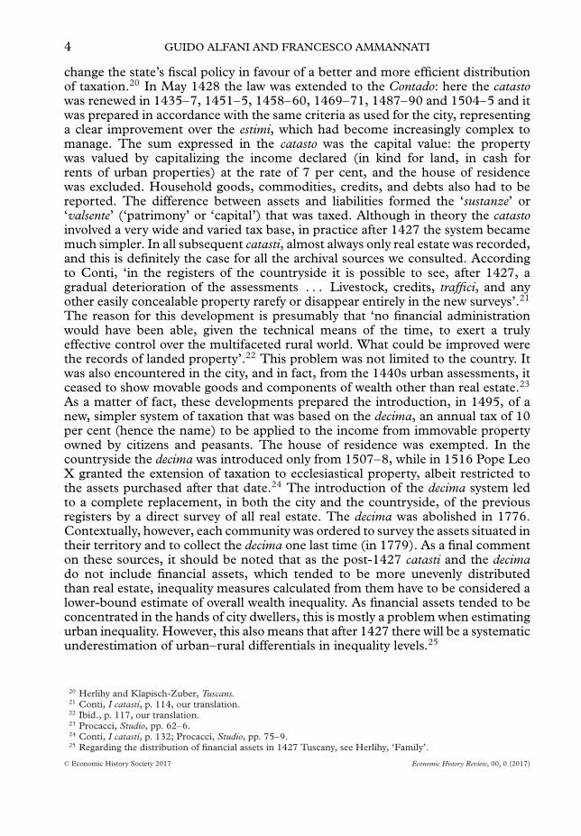
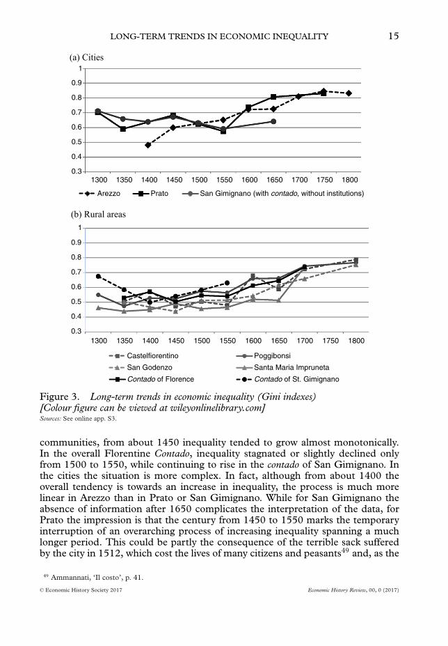
Before proceeding, we would like to provide further evidence that the trendsemerging from our descriptive analysis, and in particular the long-term tendencyfor inequality to grow, are not a statistical artefact, resulting from the change insources used. To this end, we performed a Chow test to see if there were structuralbreaks in 1427 and in 1507.52 In other words, we divided all the observationsavailable for our 11 rural communities (overall, N = 99) into three groups: thepost-Black Death estimi (1350–1426, N = 29), the catasti (1427–1506, N = 23),and the decime (after 1507, N = 47). We then calculated the coefficient of thelinear fit (�) by means of a simple linear regression (with time as the independentvariable). Differences in the coefficients related to each period did not provesignificant, and consequently we conclude that there is no structural break in1427 and 1507.53 Figure 4 provides a graphical representation of the linear fits forthe three periods. As can be seen from the figure, the passage from catasti to decimeseems particularly smooth—possibly because, as discussed above, at least in thecase of rural communities, these sources reflected basically the same fiscal base. Inthe passage from the estimi to the catasti a small drop is noticeable; however, thesource dummies we included in the regression analysis (section VI) proved non-significant.
50 Alfani, Calamities, p. 27.51 Alfani, ‘Prima’; idem, ‘Economic inequality’; Alfani and Caracausi, ‘Struttura’.52 The decima system was introduced in the countryside in 1507–8; see section I.53 Chi2 = 2.05; Prob � Chi2 = 0.36
Figure 4. Economic inequality in the Florentine Contado—looking for sources-inducedstructural breaksSources: See online app. S3.
IV
If population growth is often associated with inequality growth, during thefourteenth and fifteenth centuries we also find that huge demographic lossescaused by the Black Death are associated with inequality decline. Since ourfindings contradict older publications, the distributive effects of the Black Deathwill be analysed in some detail. Herlihy’s pioneering works are once more theunavoidable starting point, particularly those on Santa Maria Impruneta, a villagein the Florentine Contado, and on Pistoia and a village placed in the PistoieseContado, Piuvica—although, as Pistoia city statutes ordered that all old estimibe burned,54 the village is much more important than the city in Herlihy’sanalysis of the consequences of the pandemic. In Piuvica, where a rare estimodated 1243 survived, Herlihy compared it with the 1427 catasto and described awealth distribution becoming markedly more unequal after the Black Death.55 InSanta Maria Impruneta, the comparison of three pre-Black Death estimi (dated1307, 1319, and 1330) with the 1427 catasto yielded much the same result.56 Inboth instances, a higher concentration of wealth was the result of the weakeningin numbers and in collective assets of the ‘middle class’; for example, in thePistoiese area, ‘In the city and on the plain—the economic heart of the territory—
54 Herlihy, Medieval and Renaissance Pistoia, p. 185.55 Ibid., pp. 182–3.56 Herlihy, ‘Santa Maria Impruneta’, pp. 258–60.
a few families with great wealth had come to confront many with few assetsor none. The troubles of the fourteenth century had not been favorable to thegrowth or even the defense of small fortunes’.57 The process would have beenstrengthened by inheritance systems and managerial factors. Inheritance mighthave played a particularly important role, as ‘The shrinking of the populationalso undoubtedly favoured with accumulated inheritances a few lucky survivors’.58
Overall, Herlihy believed that by 1427, in the whole of Tuscany the urban (andthe rural) middle class was ‘crushed between the rich, distinguished by their hugepossession, and the poor, distinguished by their numbers’, and that probably ‘thehighly skewed distribution of wealth in the fifteenth-century was a comparativelynew development, and . . . wealth had been somewhat more evenly distributedacross the population in the thirteenth century, before the onslaught of the greatepidemics’.59
It is sufficient to look at figure 3 to note that as far as our case studies areconcerned, the situation seems to be very different from that described by Herlihy.Apparently the Black Death triggered a phase of reduction in inequality thatcontinued until about 1400 in the cities, and until about 1450 in rural communities.In all but one of the cases for which we have pre-Black Death measures of inequality,they are much lower in 1427 or around that date than before the Black Death—theexception being Antella (see table 2), possibly due to the fact that it was affectedin a milder way by the plague (137 households are recorded in 1319 and 116 in1357: a 15.3 per cent decline, which compares favourably to the 34.5 per centdecline of Santa Maria Impruneta between 1319 and 1365 and the 24.2 per centdecline of Poggibonsi between 1338 and 1357). However, even in Antella theGini trend between 1319 and 1357 is almost flat, and some decline in inequalityoccurred in the early fifteenth century. These results find support in the onlyother area for which a study of the impact of the Black Death on inequality levelshas been conducted: Piedmont. Here, the pandemic seems to be the root of afairly long phase of inequality decline, which even in the cities lasted until about1450. In Chieri, for example, a Gini index of 0.715 has been calculated for 1311,which is much higher than that calculated for 1437 (0.669), while in Cherascothe Gini of 0.630 calculated for 1350 contracted first to 0.546 in 1395–1415 andthen to 0.521 in 1447–50 (Piedmontese measures refer to inequality in real estateonly).60
The findings for Piedmont should not be considered surprising, as they are‘consistent with the hypothesis that the Black Death determined a significantincrease in real wages of skilled and unskilled workers, who consequently wouldhave had more resources to buy property’.61 Studies of labour conditions in theaftermath of the Black Death confirm that in Tuscany, wages showed a tendencyto rise,62 although Florence tried to contain the process, at least in the rural areasand—presumably—with limited success.63 In Florence there is also evidence of a
57 Herlihy, Medieval and Renaissance Pistoia, p. 189.58 Ibid., p. 190.59 Herlihy, ‘Distribution’, p. 139.60 Alfani, ‘Economic inequality’.61 Ibid., p. 1079.62 Goldthwaite, Building, pp. 317–42, app. 3; la Ronciere, ‘La condition’; idem, Prix.63 Cohn, ‘After the Black Death’, pp. 469–70.
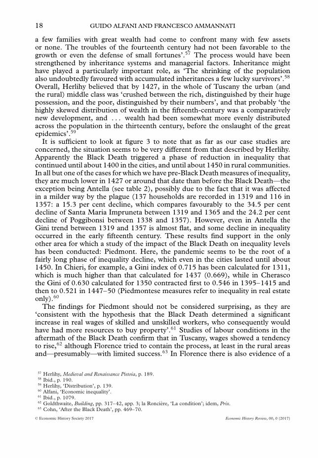
Santa Maria Impruneta (standardized)Santa Maria Impruneta (non-standardized)
Bla
ck D
eath
Figure 5. Economic inequality in Santa Maria Impruneta, 1307–1570 (Gini indexes,with or without standardization)Sources: See online app. S3.
‘huge tidal wave’ in the formation of new lineages after the Black Death, whichreflect particularly good opportunities for entering the elite.64 We could wonder,then, why Herlihy’s data seem to differ. In fact, we detected two problems withhis analysis. First of all, he compared very different points in time (separatedby more than a century in the case of Santa Maria Impruneta, and by almosttwo in Piuvica) without considering potentially crucial in-between dynamics. Forexample, as suggested by the case of Poggibonsi (figure 2), a recovery before 1427could hide the short- and medium-term egalitarian consequences of the BlackDeath. Second, he compared the thirteenth- and fourteenth-century estimi directly(without standardization) with the 1427 catasto—but the poor unable to pay taxare absent from the estimi records, while the catasto recorded almost everybody.Standardization of the sources with elimination of the propertyless from the 1427distribution (a necessary step to compare, insofar as possible, like with like) possiblyoverturns the result, exactly as in Poggibonsi where, when the individuals with ‘zerovalsente’ are taken out, the Gini calculated for 1338 (0.550) is higher than thatcalculated for 1458 (0.523) but much lower than the Gini calculated when they areincluded (0.704). In fact, after collecting the first data for the Contado, we decidedto add Santa Maria Impruneta to the original sample, replicating the research doneby Herlihy but also considering additional sources in-between those used by himand continuing the analysis until the early eighteenth century. We discovered thathere, too, including the propertyless in the calculation of the Gini from the catastodramatically alters the index values—from 0.540 to 0.660 in 1427, and from 0.491to 0.687 in 1458. Figure 5, which presents particularly dense yearly data for thefourteenth to sixteenth centuries, shows how forgetting standardization can distortinterpretation of the data (notice that if we consider the standardized data only, the
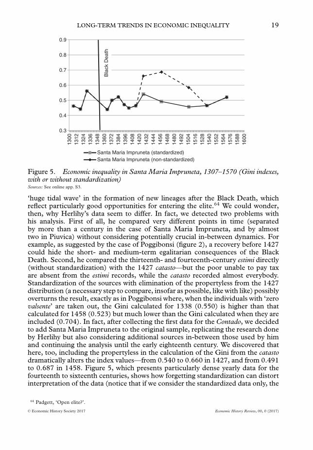
Figure 6. Wealth distribution in the pre- and post-Black Death years (Lorenz curves)Note: Lorenz curves have been drawn using the glcurve Stata package.[Colour figure can be viewed at wileyonlinelibrary.com]Sources: See online app. S3.
high point for the whole period pre-dates the Black Death, being reached in 1330when the Gini is equal to 0.561).
Our data provide strong support for the idea that the Black Death had an‘egalitarian’ impact on wealth distributions, as first hypothesized by Alfani.65 Togain a better understanding of how such an event affected the overall distributions,in figure 6 we present Lorenz curves for the four communities for which we havepre-Black Death information. For Santa Maria Impruneta and Prato we find that
the post-plague distribution lies entirely above the pre-plague one, suggesting animprovement in the relative conditions of those placed at the bottom, middle, andupper-middle parts of the distribution, to the detriment of the very richest. Overallthis is also the case in Poggibonsi, with the exception of a slight worsening ofthe relative conditions of the lower-middle levels. Only in Antella do the pre- andpost-plague distributions cross each other. While the relative share of wealth ofthe bottom 50 per cent of the distribution increases, the upper-middle levels loseposition to the advantage of the top 10 per cent (the overall result is an almostunchanging Gini). Notice that in all cases, changes in the Ginis were coupled withan increase in per capita (or per household) property determined by the hugepopulation decline—so that the society emerging from the Black Death was bothmore egalitarian and ‘richer’.
It is quite clear from our data that the Black Death was able to alter deeply thesocial-economic structures of medieval Tuscany, partly due to the pure magnitudeof the shock, and partly because Tuscan society was totally unprepared for thisnew threat. In particular, the ‘unmitigated’ partible inheritance system that existedon the eve of the Black Death caused, at least in the short run, a (undesired)patrimonial fragmentation (as patrimonies were divided evenly among inheritors)that surely contributed to the quick decline in inequality immediately after thepandemic. However, the impact of the plague on inequality levels following theBlack Death is less clear, mostly due to the adaptation that occurred in inheritancepractices, as has been argued for early modern Piedmont66 and, again for reasonsof synthesis, this will not be discussed in this article. We will now analyse in greaterdetail the distribution of wealth in medieval and early modern Tuscany, payingparticular attention to the problems presented by the absence of the propertylessfrom most of our sources.
V
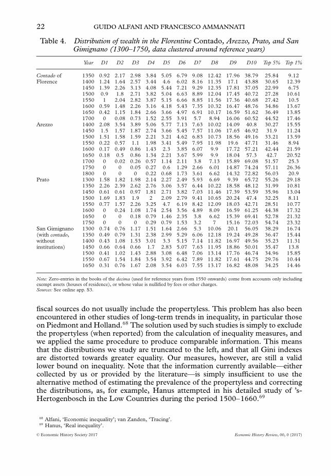
Several studies have shown that the Tuscan society of the late middle ages wasprofoundly unequal. In fourteenth- and fifteenth-century Florence, a huge massof poor families were in close contact with a small number of people enjoyingimmense wealth, and in the secondary cities of the state the concentration of richeswas equally strong.67 The situation in the Florentine Contado does not seem verydifferent. Table 4 provides key information about the distribution of wealth indifferent parts of the Florentine state.
The distribution of wealth by deciles shows the extraordinary concentration ofproperty in the hands of a few people. In San Gimignano, from the middle ages tomodern times, 10 per cent of the richest taxpayers held on firmly to about 50 percent of the wealth. In the Contado of Florence, about 40 per cent was owned by therichest 10 per cent of the population, a percentage that exceeded 50 per cent in theseventeenth century and reached 60 per cent at the beginning of the eighteenth.Shares are even higher for the very richest of Arezzo and Prato.
While the top of the distribution is reflected very well by our sources, it is muchmore difficult to get a clear picture of the bottom, as medieval and early modern
66 Alfani, ‘Effects’; idem, ‘Economic inequality’.67 Herlihy, ‘Distribution’; Herlihy and Klapisch-Zuber, Tuscans, pp. 97–102; Stella, La revolte, pp. 185–92.
Note: Zero-entries in the books of the decima (used for reference years from 1550 onwards) come from accounts only includingexempt assets (houses of residence), or whose value is nullified by fees or other charges.Sources: See online app. S3.
fiscal sources do not usually include the propertyless. This problem has also beenencountered in other studies of long-term trends in inequality, in particular thoseon Piedmont and Holland.68 The solution used by such studies is simply to excludethe propertyless (when reported) from the calculation of inequality measures, andwe applied the same procedure to produce comparable information. This meansthat the distributions we study are truncated to the left, and that all Gini indexesare distorted towards greater equality. Our measures, however, are still a validlower bound on inequality. Note that the information currently available—eithercollected by us or provided by the literature—is simply insufficient to use thealternative method of estimating the prevalence of the propertyless and correctingthe distributions, as, for example, Hanus attempted in his detailed study of ’s-Hertogenbosch in the Low Countries during the period 1500–1660.69
68 Alfani, ‘Economic inequality’; van Zanden, ‘Tracing’.69 Hanus, ‘Real inequality’.
Only in some exceptional circumstances, and in particular for the period coveredby the catasti, can we measure the prevalence of the propertyless. In 1427 the lawallowed Florentine citizens to deduct 200 florins for each member of the family, asum which could have reduced even a good fortune to zero.70 This rule, however,was not extended to the taxpayers of the Contado, who only shared with the citizensthe deduction for the house of residence. Luckily, the sources indicate the value ofthese properties, even if they were not included in the calculation of the total taxableamount, and we were able to incorporate them in our reconstruction. Using thedata of our 11 communities of the Contado for the years 1450 and 1500, the overallpercentage of taxpayers with a valsente of 0 (without considering deductions) is33.1 and 30.6 per cent respectively. Earlier research showed that in 1427, net ofdeductions, 21 per cent of households of the whole of rural Tuscany were recordedin the catasto with a valsente of 0, while almost two-thirds were taxable at a valueof under 100 florins. In the central area of the Contado, where more than half ofthe land was involved in sharecropping, the percentage of taxpayers with a valsenteof 0 was about 50 per cent.71 Including deductions obviously inflates these 1427measures. For example, for the city of Florence in that year, available estimates ofpropertyless citizens range from 28.8 per cent72 to 31 per cent—but these figuresare net of deductions and, in fact, those who did not have anything at all regardlessof deductions were just 14 per cent.73 For Prato, we only have estimates net ofdeductions, according to which the propertyless would constitute 17.9 per centand 32.2 per cent respectively in the catasti of 1428 and of 1487. For this city, wealso have a figure from the estimo of 1372, when 37.6 per cent of households hadno taxable property.
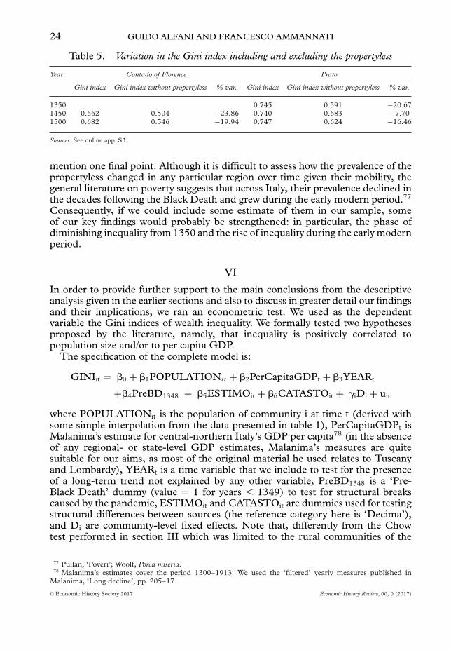
Overall, it seems that the part of population excluded by the Tuscan fiscalsources might have been exceptionally high compared to other areas of Italy.In Piedmont, for example, the scattered information available suggests that thepopulation entirely devoid of real estate varied, in the period 1393–1613, withinthe fairly tight band of 8.5 to 11 per cent, both in cities and in rural areas.74 Thisdifference was probably due, at least to a large degree, to the relative abundanceof sharecropping and to the system of deductions used in the Florentine state. Asa consequence, the distortion towards equality of our estimates is also relativelylarge. As shown by table 5, the decrease in the Gini values caused by the exclusionof the propertyless is around 20 per cent, except in the case of Prato in 1450, wherethe decrease was much lower, at 7.7 per cent—very close to the 7.1 per cent thatcan be calculated from data published by van Zanden for the Florentine catasto of1457.75 A decrease of 11.7 per cent has been measured instead by excluding thepropertyless from the calculation of the Gini index in Ivrea, in north-western Italy,in 1613.76
We leave to future research a more systematic analysis and measurement of theprevalence of poverty in late medieval and early modern Tuscany. We will only
70 Conti, L’imposta.71 Herlihy and Klapisch-Zuber, Tuscans, pp. 118–20.72 de Roover, Il banco, p. 42.73 Herlihy and Klapisch-Zuber, Tuscans, p. 100.74 Alfani, ‘Economic inequality’.75 van Zanden, ‘Tracing’, p. 645.76 Alfani and Caracausi, ‘Struttura’, pp. 199, 203.
mention one final point. Although it is difficult to assess how the prevalence of thepropertyless changed in any particular region over time given their mobility, thegeneral literature on poverty suggests that across Italy, their prevalence declined inthe decades following the Black Death and grew during the early modern period.77
Consequently, if we could include some estimate of them in our sample, someof our key findings would probably be strengthened: in particular, the phase ofdiminishing inequality from 1350 and the rise of inequality during the early modernperiod.
VI
In order to provide further support to the main conclusions from the descriptiveanalysis given in the earlier sections and also to discuss in greater detail our findingsand their implications, we ran an econometric test. We used as the dependentvariable the Gini indices of wealth inequality. We formally tested two hypothesesproposed by the literature, namely, that inequality is positively correlated topopulation size and/or to per capita GDP.
The specification of the complete model is:
GINIit = �0 + �1POPULATIONi t + �2PerCapitaGDPt + �3YEARt
+�4PreBD1348 + �5ESTIMOit + �6CATASTOit + �iDi + uit
where POPULATIONit is the population of community i at time t (derived withsome simple interpolation from the data presented in table 1), PerCapitaGDPt isMalanima’s estimate for central-northern Italy’s GDP per capita78 (in the absenceof any regional- or state-level GDP estimates, Malanima’s measures are quitesuitable for our aims, as most of the original material he used relates to Tuscanyand Lombardy), YEARt is a time variable that we include to test for the presenceof a long-term trend not explained by any other variable, PreBD1348 is a ‘Pre-Black Death’ dummy (value = 1 for years � 1349) to test for structural breakscaused by the pandemic, ESTIMOit and CATASTOit are dummies used for testingstructural differences between sources (the reference category here is ‘Decima’),and Di are community-level fixed effects. Note that, differently from the Chowtest performed in section III which was limited to the rural communities of the
77 Pullan, ‘Poveri’; Woolf, Porca miseria.78 Malanima’s estimates cover the period 1300–1913. We used the ‘filtered’ yearly measures published in
Notes: Standard errors are clustered per community and are in parentheses.∗∗∗
p�0.01,∗∗
p�0.5,∗p�0.1. Models (1) to (4) cover
the whole period 1300–1800. Models (5) and (6) are balanced panels covering only the period 1350–1700.Sources: See text and online app. S3.
Contado, the variables ESTIMOit and CATASTOit are not equivalent to timedummies, as for the Distretto we also used some estimi which date from after 1427,when the catasti system was introduced in the Contado (see online appendix S1).As a consequence, their inclusion does not test for structural breaks in 1427 and1507, but for structural differences related to different sources partly overlappingin time. Finally, in some specifications without fixed effects, we add the time-invariant dummy URBANi to test for structural differences between cities andrural communities.
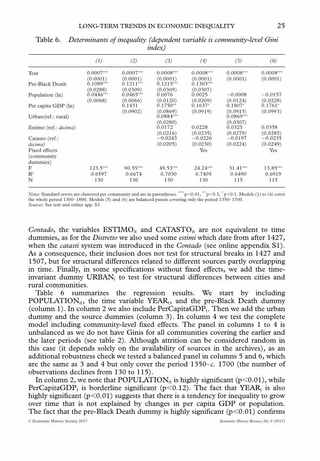
Table 6 summarizes the regression results. We start by includingPOPULATIONit, the time variable YEARt, and the pre-Black Death dummy(column 1). In column 2 we also include PerCapitaGDPt. Then we add the urbandummy and the source dummies (column 3). In column 4 we test the completemodel including community-level fixed effects. The panel in columns 1 to 4 isunbalanced as we do not have Ginis for all communities covering the earlier andthe later periods (see table 2). Although attrition can be considered random inthis case (it depends solely on the availability of sources in the archives), as anadditional robustness check we tested a balanced panel in columns 5 and 6, whichare the same as 3 and 4 but only cover the period 1350–c. 1700 (the number ofobservations declines from 130 to 115).
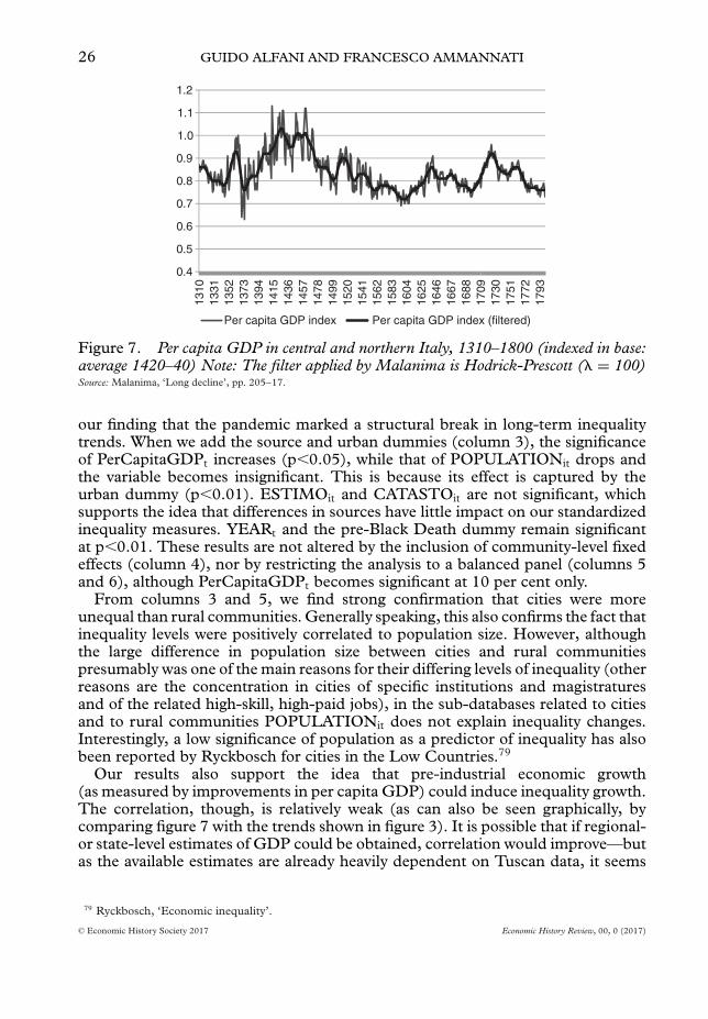
Per capita GDP index Per capita GDP index (filtered)
Figure 7. Per capita GDP in central and northern Italy, 1310–1800 (indexed in base:average 1420–40) Note: The filter applied by Malanima is Hodrick-Prescott (� = 100)Source: Malanima, ‘Long decline’, pp. 205–17.
our finding that the pandemic marked a structural break in long-term inequalitytrends. When we add the source and urban dummies (column 3), the significanceof PerCapitaGDPt increases (p�0.05), while that of POPULATIONit drops andthe variable becomes insignificant. This is because its effect is captured by theurban dummy (p�0.01). ESTIMOit and CATASTOit are not significant, whichsupports the idea that differences in sources have little impact on our standardizedinequality measures. YEARt and the pre-Black Death dummy remain significantat p�0.01. These results are not altered by the inclusion of community-level fixedeffects (column 4), nor by restricting the analysis to a balanced panel (columns 5and 6), although PerCapitaGDPt becomes significant at 10 per cent only.
From columns 3 and 5, we find strong confirmation that cities were moreunequal than rural communities. Generally speaking, this also confirms the fact thatinequality levels were positively correlated to population size. However, althoughthe large difference in population size between cities and rural communitiespresumably was one of the main reasons for their differing levels of inequality (otherreasons are the concentration in cities of specific institutions and magistraturesand of the related high-skill, high-paid jobs), in the sub-databases related to citiesand to rural communities POPULATIONit does not explain inequality changes.Interestingly, a low significance of population as a predictor of inequality has alsobeen reported by Ryckbosch for cities in the Low Countries.79
Our results also support the idea that pre-industrial economic growth(as measured by improvements in per capita GDP) could induce inequality growth.The correlation, though, is relatively weak (as can also be seen graphically, bycomparing figure 7 with the trends shown in figure 3). It is possible that if regional-or state-level estimates of GDP could be obtained, correlation would improve—butas the available estimates are already heavily dependent on Tuscan data, it seems
reasonable to assume that changes in per capita GDP could explain only a fairlylimited part of the tendency for inequality to grow in time. Indeed, the literature onthe Florentine state agrees in describing the early modern period, from at least thefirst decades of the seventeenth century, as one of decline following a glorious ‘early’Renaissance when Florence was one of the main economic centres of Europe.80
Our regression analysis, then, provides evidence that, after the decline caused bythe Black Death, something that was not economic growth was driving a continuousincrease in inequality: on average, in the period 1300–1800 and independentlyfrom the Black Death break, our time variable accounts for an increase in theGini index between 0.07 and 0.08 points every hundred years. Consequently, ourarticle supports recent works suggesting that during the early modern period,in many areas of Europe economic inequality was growing even in times ofeconomic stagnation or decline. In Italy, this would be the case of the Sabaudianstate (Piedmont) in the north-west during the seventeenth century and possibly(if some recently presented preliminary results are confirmed) also of other areas,such as the Republic of Venice in the north-east.81 Beyond Italy, inequality growthin periods of economic stagnation/decline seems to have happened in the SouthernLow Countries (Belgium) and in central Spain.82 Only for Portugal do we havestrong evidence of a correlation between early modern economic stagnation and(income) inequality decline.83
Generally speaking, our regression analysis suggests that in order to accountfully for the trend we detected, we need to focus on variables that are notcurrently comprised in the model—variables whose joint effect is captured bythe YEARt variable. This requires more research, possibly incorporating micro-level case studies, and is beyond the aims of this article. We can, however, pointout at least two other areas that would be worthy of further exploration. Oneis demography—as has been shown, on the basis of a micro-analysis of Ivrea inPiedmont, that in cities inequality growth could result from immigration of poorrural dwellers even in the presence of a stable overall population (as the naturalgrowth rates in early modern cities were usually negative).84 A similar point has alsorecently been made for ’s-Hertogenbosch in the Low Countries.85 The impact ofout-migration and population pressure on inequality in rural areas is, however,more complex to assess, as shown by other studies.86 Additionally, especiallyduring the early modern period, in rural areas population pressure on the availableresources determined the crisis of small holdings, a process further exhacerbated bythe partible inheritance system, which determined the fragmentation of the originalplot among an increasingly larger number of heirs—making property fragile andmore liable to be sold. This was suggested by a classic work by le Roy Ladurieon the Languedoc in France, where an increasing concentration of wealth (land)
resulted from a kind of ‘natural selection’ favouring the main owners,87 and hasalso been found in Piedmont and elsewhere in Italy.88 Presumably Tuscany was noexception, as the population of the region increased steadily from about 561,000in 1500, to 885,000 in 1600, to 936,000 in 1700, reaching 1,270,000 in 1800.89
Another factor to consider is the institutional framework, and in particular theevolution of fiscal systems underpinning the rise of the fiscal state. In his studyof the Sabaudian state in the seventeenth century, Alfani suggested that fiscaldevelopments allowed the extraction of more resources—and, in the presence ofinegalitarian redistribution, this also made it possible to ‘extract’ more inequalityfrom the theoretical maximum represented by the Inequality Possibility Frontier.90
More recently, the deepening of regressive taxation has been singled out as apossible causative factor of inequality growth in the Low Countries.91 Futureresearch will assess whether processes of this kind could also have played a role inpromoting inequality growth in Tuscany.
VII
This article has presented a broad picture of economic inequality from about 1300to about 1800 in the Florentine state (Tuscany), an area characterized by theavailability of exceptionally rich and ancient sources. To date, Tuscany is one ofthe very few regions of Europe to have been the object of a comprehensive attemptto study inequality in the long run. Many of our findings are consistent with thoseof earlier studies, particularly Alfani’s work on Piedmont and van Zanden’s onHolland.92 In all three regions, a continuous increase in inequality has been foundfrom at least the sixteenth century onwards. The interpretation of the process,however, varies: van Zanden connected it to pre-industrial economic growth,while Alfani suggested that this explanation was not sufficient for Piedmont, whoseeconomy stagnated during the seventeenth century when inequality continued togrow. In Piedmont, other factors, including institutional (the development of amore ‘extractive’ fiscal state) and demographic ones, allowed for rises in inequalityeven in the absence of significant economic growth.93 The case of Tuscany supportsthe hypothesis that in early modern Europe, inequality was also growing in manyareas that were economically stagnating. Possibly also in Tuscany inequality growthwas at least partially driven by changes in the institutional framework. This is,however, an aspect on which further research is needed.
The middle ages, although overall characterized by economic growth, were nota period of continuous increase in economic inequality. The Black Death, in fact,seems to have triggered a phase of declining inequality that lasted about a century.Very similar dynamics were found in the only other study—that on Piedmont—which allows for a comparison. Interestingly, until now the only attempt to uncover
87 le Roy Ladurie, Les paysans, p. 572.88 Alfani, ‘Economic inequality’; idem, Calamities, pp. 76–7.89 Figures from Breschi and Malanima, ‘Demografia’.90 Alfani, ‘Economic inequality’. For the notion of extraction of inequality, see Milanovic, Lindert, and
the impact of the Black Death on Tuscan property structures and general economicinequality levels suggested exactly the contrary.94 We partly replicated this earlierwork, thereby detecting the probable cause of a misinterpretation of the data.Therefore, on the grounds of all the evidence currently available, we can arguethat among the consequences of the Black Death in Europe, a significant (albeittemporary) decline in economic inequality must also be counted.
Date submitted 13 November 2014Revised version submitted 3 August 2016Accepted 7 August 2016
DOI: 10.1111/ehr.12471
Footnote referencesAlfani, G., ‘Prima della curva di Kuznets: stabilita e mutamento nella concentrazione di ricchezza e proprieta
in eta moderna’, in G. Alfani and M. Barbot, eds., Ricchezza, valore, proprieta in Eta preindustriale. 1400–1850(Venice, 2009), pp. 143–68.
Alfani, G., ‘Wealth inequalities and population dynamics in northern Italy during the early modern period’,Journal of Interdisciplinary History, 40 (2010), pp. 513–49.
Alfani, G., ‘The effects of plague on the distribution of property: Ivrea, northern Italy 1630’, Population Studies,64 (2010), pp. 61–75.
Alfani, G., Calamities and the economy in Renaissance Italy. The Grand Tour of the Horsemen of the Apocalypse(Basingstoke, 2013).
Alfani, G., ‘Economic inequality in northwestern Italy: a long-term view (fourteenth to eighteenth centuries)’,Journal of Economic History, 75 (2015), pp. 1058–96.
Alfani, G. and Barbot, M., eds., Ricchezza, valore, proprieta in Eta preindustriale. 1400–1850 (Venice, 2009).Alfani, G. and Caracausi, A, ‘Struttura della proprieta e concentrazione della ricchezza in ambiente urbano: Ivrea
e Padova, secoli XV–XVII’, in G. Alfani and M. Barbot, eds., Ricchezza, valore, proprieta in Eta preindustriale.1400–1850 (Venice, 2009), pp. 185–209.
Alfani, G. and di Tullio, M., ‘Dinamiche di lungo periodo della disuguaglianza in Italia settentrionale: una notadi ricerca’, Dondena working paper, 71 (2015).
Alfani, G. and Frigeni, R., ‘Inequality (un)perceived: the emergence of a discourse on economic inequality fromthe middle ages to the age of revolutions’, Journal of European Economic History, 45 (2016), pp. 21–66.
Alvaredo, F., Atkinson, A. B., Picketty, T., and Saez, E., ‘The top 1 percent in international and historicalperspective’, Journal of Economic Perspectives, 27, 3 (2013), pp. 3–20.
Ammannati, F., ‘Florentine woollen manufacture in the sixteenth century: crisis and new entrepreneurialstrategies’, Business and Economic History On-Line, 7 (2009), pp. 1–9.
Ammannati, F., ‘Il costo della liberta nei conti di alcuni personaggi’, Prato Storia e Arte, 112 (2012), pp. 39–51.Atkinson, A. B., Picketty, T., and Saez, E., ‘Top incomes in the long run of history’, Journal of Economic Literature,
49 (2011), pp. 3–71.Barbadoro, B., Le finanze della Repubblica Fiorentina. Imposta diretta e debito pubblico fino all’istituzione del Monte
(Florence, 1929).Boudjaaba, F., ‘La distribuzione delle fortune fondiarie in Francia alla fine dell’Ancien Regime: un approccio
dinamico a partire dall’esempio della Normandia’, in G. Alfani and M. Barbot, eds., Ricchezza, valore, proprietain Eta preindustriale. 1400–1850 (Venice, 2009), pp. 371–90.
Breschi, M. and Malanima, P., ‘Demografia ed economia in Toscana: il lungo periodo (secoli XIV–XIX)’, in M.Breschi and P. Malanima eds., Prezzi, redditi, popolazione in Italia: 600 anni (dal secolo XIV al secolo XX) (Udine,2002), pp. 109–42.
Canbakal, H., ‘Wealth and inequality in Ottoman Bursa, 1500–1840’, paper presented at the Economic HistorySociety Annual Conference (York, 5–7 April 2013).
Carmona, M., ‘La Toscane face a la crise de l’industrie laniere: techniques et mentalites economiques aux XVIet XVII siecles’, in M. Spallanzani, ed., Produzione commercio e consumo dei panni di lana, nei secoli 12-18–Attidella seconda Settimana di studio, 10–16 aprile 1970 (Florence, 1976), pp. 151–68.
Casini, B., Il catasto di Livorno del 1427–29 (Pisa, 1984).Cohn, S. K., jr., ‘After the Black Death: labour legislation and attitudes towards labour in late-medieval western
Europe’, Economic History Review, 60 (2007), pp. 486–512.
94 Herlihy, Medieval and Renaissance Pistoia; idem, ‘Santa Maria Impruneta’.
Conti, E., La formazione della struttura agraria moderna nel Contado fiorentino, III, part 2°, Monografie e tavolestatistiche (secoli X–XIX) (Rome, 1965).
Conti, E., I catasti agrari della Repubblica fiorentina e il catasto particellare toscano (secoli XIV-XIX) (Rome, 1966).Conti, E., L’imposta diretta a Firenze nel Quattrocento (Rome, 1984).Curtis, D. R., ‘Florence and its hinterlands in the late middle ages: contrasting fortunes in the Tuscan countryside,
1300–1500’, Journal of Medieval History, 38 (2012), pp. 472–99.Dini, B., Arezzo intorno al 1400. Produzioni e mercato (Arezzo, 1984).Fasano Guarini, E., Lo stato mediceo di Cosimo I (Florence, 1973).Fiumi, E., ‘La demografia fiorentina nelle pagine di Giovanni Villani’, Archivio Storico Italiano, CVIII, 1 (1950),
pp. 78–155.Fiumi, E., Storia economica e sociale di S. Gimignano (Florence, 1961).Fiumi, E., Demografia, movimento urbanistico e classi sociali in Prato dall’eta comunale ai tempi moderni (Florence,
1968).Garcia Montero, H., ‘Long-term trends in wealth inequality in Catalonia 1400-1800: initial results’, Dondena
working paper 79 (2015).Goldthwaite, R. A., The building of Renaissance Florence. An economic and social history (Baltimore, Md., 1980).Goldthwaite, R. A., The economy of Renaissance Florence (Baltimore, Md., 2009).Hanus, J., ‘Income mobility and economic growth in the Low Countries in the sixteenth century’, Journal of
European Economic History, 41 (2012), pp. 15–49.Hanus, J., ‘Real inequality in the early modern Low Countries: the city of ’s-Hertogenbosch, 1500–1660’,
Economic History Review, 66 (2013), pp. 733–56.Herlihy, D., Medieval and Renaissance Pistoia (New Haven, Conn., and London, 1967).Herlihy, D., ‘Santa Maria Impruneta: a rural commune in the late middle ages’, in N. Rubinstein, ed., Florentine
studies: politics and society in Renaissance Florence (1968), pp. 242–76.Herlihy, D., ‘Family and property in Renaissance Florence’, in H. A. Miskimin, D. Herlihy, and A. L. Udovitch,
eds., The medieval city (New Haven, Conn., 1977), pp. 3–24.Herlihy, D., ‘The distribution of wealth in a Renaissance community: Florence 1427’, in P. Abrams and E. A.
Wrigley, eds., Towns in societies. Essays in economic history and historical sociology (Bristol, 1978), pp. 131–57.Herlihy, D. and Klapisch-Zuber, C., Tuscans and their families: a study of the Florentine catasto of 1427 (New Haven,
Conn., and London, 1985).Hoffman, P. T., Jacks, D., Levin, P. A., and Lindert, P. H., ‘Real inequality in Europe since 1500’, Journal of
Economic History, 62 (2002), pp. 322–55.Kuznets, S., ‘Economic growth and income inequality’, American Economic Review, 45, 1 (1955), pp. 1–28.de la Ronciere, C.-M., ‘La condition des salaries a Florence au XIVe siecle’, in Il Tumulto Dei Ciompi. Un momento
di storia fiorentina ed europea (Florence, 1981), pp. 13–40.de la Ronciere, C.-M., Prix et salaires a Florence au XIVe siecle (1280–1380) (Rome, 1982).le Roy Ladurie, E., Les paysans de Languedoc (Paris, 1966).Lindert, P. H., ‘Making the most of capital in the 21st century’, National Bureau of Economic Research working
paper no. 20232 (2014).Lindert, P. H. and Williamson, J. G., American inequality: a macro economic history (New York, 1980).Malanima, P., La decadenza di un’economia cittadina. L’industria di Firenze nei secoli XVI–XVIII (Bologna, 1982).Malanima, P., ‘The long decline of a leading economy: GDP in central and northern Italy, 1300–1913’, European
Review of Economic History, 15 (2011), pp. 169–219.Mazzotti, O., ‘Alcune considerazioni su frammentazione e concentrazione della proprieta in area romagnola alla
fine del settecento’, in G. Alfani and M. Barbot, eds., Ricchezza, valore, proprieta in Eta preindustriale. 1400–1850 (Venice, 2009), pp. 239–53.
Milanovic, B., Lindert, P. H., and Williamson, J. G., ‘Pre-industrial inequality’, Economic Journal, 121 (2011),pp. 255–72.
Nicolini, E. A. and Ramos Palencia, F., ‘Comparing income and wealth inequality in pre-industrial economies:lessons from 18th-century Spain’, European Historical Economics Society working papers in economic historyno. 95 (2016).
Padgett, J., ‘Open elite? Social mobility, marriage, and family in Florence, 1282–1494’, Renaissance Quarterly, 63(2010), pp. 357–411.
Pagnini del Ventura, G. F., Della decima e di varie altre gravezze imposte dal Comune di Firenze, 4 vols. (Lisbon andLucca, 1766; repr. Bologna, 1967).
del Panta, L., Una traccia di storia demografica della Toscana nei secoli XVI–XVIII (Florence, 1974).Piketty, T., Capital in the twenty-first century (Cambridge, 2014).Piketty, T., Postel-Vinay, G., and Rosenthal, J.-L., ‘Wealth concentration in a developing economy: Paris and
France, 1807–1994’, American Economic Review, 96, 1 (2006), pp. 236–56.Prados de la Escosura, L., ‘Inequality and poverty in Latin America: a long-run exploration’, in T. J. Hatton,
K. H. O’Rourke, and A. M. Taylor, eds., The new comparative economic history (Cambridge, Mass., 2007), pp.291–315.
Prados de la Escosura, L., ‘Inequality, poverty and the Kuznets curve in Spain, 1850–2000’, European Review ofEconomic History, 12 (2008), pp. 287–324.
Procacci, U., Studio sul Catasto fiorentino (Florence, 1996).Pullan, B., ‘Poveri, mendicanti e vagabondi (secoli XIV–XVII)’, in Storia d’Italia. Annali, 1: Dal feudalesimo al
capitalismo (Turin, 1978), pp. 51–83.Reis, J., ‘Deviant behaviour? Inequality in Portugal 1565–1770’, Cliometrica (forthcoming).de Roover, R., Il banco Medici dalle origini al declino (1397–1494) (Florence, 1970).Rossi, N., Toniolo, G., and Vecchi, G., ‘Is the Kuznets curve still alive? Evidence from Italian household budgets,
1881–1961’, Journal of Economic History, 61 (2001), pp. 904–25.Ryckbosch, W., ‘A consumer revolution under strain. Consumption, wealth and status in eighteenth-century Aalst
(Southern Netherlands)’ (unpub. Ph.D. thesis, Univ. of Antwerp and Univ. of Ghent, 2012).Ryckbosch, W., ‘Economic inequality and growth before the industrial revolution: the case of the Low Countries
(fourteenth to nineteenth centuries)’, European Review of Economic History, 20 (2016), pp. 1–22.Santiago-Caballero, C., ‘Income inequality in central Spain, 1690–1800’, Explorations in Economic History, 48
(2011), pp. 83–96.Santiago-Caballero, C. and Fernandez, E., ‘Income inequality in Madrid, 1500–1850’, paper presented at the
Economic History Society Annual Conference (York, 5–7 April 2013).Soltow, L. and van Zanden, J. L., Income and wealth inequality in the Netherlands, 16th–20th centuries (Amsterdam,
1998).Stella, A., La revolte des Ciompi. Les hommes, les lieux, le travail, Recherches d’histoire et de sciences sociales (Paris,
1993).Williamson, J. G., Did British capitalism breed inequality? (Boston, Mass., 1985).Woolf, S. J., Porca miseria. Poveri e assistenza nell’Eta moderna (Bari, 1988).van Zanden, J. L., ‘Tracing the beginning of the Kuznets curve: western Europe during the early modern period’,
Economic History Review, XLVIII (1995), pp. 643–64.
Supporting information
Additional Supporting Information may be found in the online version of thisarticle at the publisher’s web-site:
Appendix S1. Additional information about sources and data collection in theContado and in the Distretto of FlorenceAppendix S2. The spread of Florentine propertyAppendix S3. Archival sources